Abstract
Settlements and settlement systems are key arenas of human–environment interaction, and reconstructing their spatial patterns is essential for understanding historical socio-environmental dynamics. Using the Complete Map of the Great Qing Empire (1905), this study employs digital extraction and spatial-statistical analysis to examine the nationwide settlement system of late Qing China. The results reveal that: (1) The system features dispersed high-level settlements and highly clustered low-level ones; provincial and prefectural cities follow administrative divisions, while counties, towns, and villages display strong spatial self-organization. (2) Mid-to high-level systems exhibit hierarchical fractures, whereas low-level settlements conform to Zipf’s law, highlighting the regularity and universality of grassroots networks. (3) Road accessibility, slope, and elevation significantly influence settlement hierarchy, whereas river proximity plays a limited role—indicating greater dependence on transportation and terrain adaptability. Overall, the study elucidates the spatial structure and formative mechanisms of the Qing settlement system and provides empirical insights into the evolution of surface patterns and regional resilience since the modern era.
1. Introduction
In geography, a settlement refers to a community of people living in a place, and a settlement system is the hierarchical arrangement of such communities by size, population, and services within a region. Meanwhile, settlements and settlement systems have long been the subject of multidisciplinary attention. As the primary spatial carriers of human activities on the Earth’s surface, their patterns and evolutions often embody profound social, cultural, economic, and political significances, while also serving as important indicators of environmental changes [1,2,3]. Long-term studies of settlements can help us understand surface patterns and the underlying interactions between human-social systems, holding significant value in revealing surface processes, social resilience, human-land relationships, spatial economic structures, and cultural patterns [4].
Existing studies have explored the relationships between settlements and socio-environmental dynamics across various regions and periods. Mortensen (1970s) examined early settlements and population dynamics in Egypt, integrating burial and anthropological data to reveal the profound influences of environmental and social factors on settlement selection and population structure [5]. Zhang et al. (2005), drawing on archeological and environmental data from the Yangtze River Delta, demonstrated the decisive role of climate and hydrological changes in the development of Neolithic cultures, cultural interruptions, and the rise and fall of civilizations [6]. Shennan (1993), combining archeological and chronological data, unveiled major transformations in Central European settlements and social structures from 3500 to 1500 BC, including population fluctuations, shifts in gender relations, and the linkages between metallurgical developments and the emergence of chiefdoms [7]. Easterlin (1976), using the northern United States as a case study, revealed the phased expansion and stagnation of farm populations under land resource constraints, thereby validating the applicability of Malthusian population theory in historical contexts [8]. Li et al. (2022), taking the mountainous regions of western Hunan as an example, illustrated the spatial characteristics of 18th-century settlement expansion and its socio-cultural roots, driven by policy shifts, population dynamics, and agricultural innovations [9].
From the perspective of current research, most scholars have focused on the spatiotemporal evolution of settlements and populations, or leveraged them to investigate multidimensional themes—such as social, environmental, economic, and cultural dimensions—in historical periods. However, there remains insufficient attention to the internal structures and interconnectivities of settlement systems themselves [10,11,12]. In fact, as early as the last century, Skinner (1964) demonstrated the integrative role of market networks in traditional agricultural societies through an analysis of China’s rural marketing system, emphasizing that markets function not only as economic mechanisms but also as critical linkages in village-community social structures and broader societal integration [13]. This perspective offers important methodological insights for examining the spatial structures of historical settlement systems. The diversity of Chinese history, coupled with its abundant documentary records, provides unparalleled conditions for such research. In recent years, with the rapid advancement of interdisciplinary research, studies of settlement evolution have expanded beyond traditional pattern analysis to encompass broader themes such as cultural and environmental adaptation [14]. The temporal dimension remains a fundamental aspect of geographical inquiry [15] and is equally crucial in settlement geography and development studies [16]. Recently, scholars have increasingly emphasized the importance of uncovering or reconstructing settlement patterns using new data sources and methods [17,18,19]. Historical maps, in particular, have emerged as valuable data sources for revealing spatial structures prior to the remote-sensing era (before the 1960s). With the growing integration of digital humanities and artificial intelligence, their potential is being further recognized and explored [20,21,22].
Building on this foundation, the present study employs the preserved Complete Map of the Great Qing Empire (Da Qing Digguo Quantu, 1905) from the late Qing Dynasty to digitally reconstruct the settlement system across mainland China at the turn of the 20th century. Specifically, this study addresses three core questions: (1) What were the spatial distribution characteristics of the settlement system in late Qing China? (2) How were settlement hierarchies shaped by environmental and topographic factors? (3) How can historical maps, such as the Complete Map of the Great Qing Empire, be digitally reconstructed to derive reliable historical settlement data and assess their accuracy?
By addressing these questions, this study not only reconstructs the hierarchical structure of historical settlements on a national scale but also provides a methodological framework for integrating historical cartographic data into quantitative land-system analyses.
This contributes to the broader field of land science by linking spatial reconstruction, environmental adaptation, and socio-political organization within a long-term human–land relationship perspective.
2. Materials and Methods
2.1. Map Digitization and Data Extraction
The Complete Map of the Great Qing Empire was published by the Commercial Press in Shanghai in the 31st year of the Guangxu reign (1905), comprising 25 maps in total, including one national map and 24 provincial and regional maps. As one of the significant achievements in late Qing cartography, it is regarded both as a representative of the transition from traditional Chinese cartography to modern cartography and as a typical case in the compilation of provincial maps following the Opium Wars [23,24]. Its content is relatively detailed, employing up to 15 distinct symbols for settlements, while also marking elements such as treaty ports, railways, and telegraph lines, thereby reflecting the latest changes in the social and economic landscape of the time.
One of the objectives of this study is to digitally extract settlement information from the map. Referencing established processing methods from prior research, the central meridian was set at 116.4283° [22], with latitudes based on the original map notations. Under the ArcGIS 10.8 environment, manual georeferencing and rectification were performed for all map sheets. Historical maps were rectified using second-and third-order polynomial geometric transformations. For each province, 7–31 ground control points (GCPs) were selected from each map. The provincial RMS registration errors are all less than 0.0139, with a national composite RMS of 0.0619. Most RMS values are below 0.01, indicating satisfactory geometric consistency sufficient for province-level analyses of land use and topography. Detailed transformation parameters and accuracy statistics are listed in Appendix A Table A1.
Subsequently, extraction was conducted according to the legend standards, categorized as provincial capitals—prefectural cities—directly administered departments—directly administered subprefectures—subprefectures—counties (including indigenous subprefectures and indigenous departments), treaty ports, postal stations, general settlements, and larger settlements (Figure 1) (Appendix A). Calculations indicate that the average positioning error for provincial capitals is approximately 14 km, with notably larger deviations for certain frontier cities such as Urumqi and Lhasa; detailed results are provided in Appendix B.
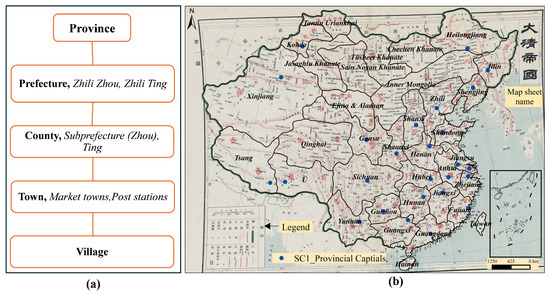
Figure 1.
Research Path (a) and Digitization Effect (National Map Sheet) (b) (The basemap shows the visualization of the nationwide map sheets after georeferencing of the atlas).
2.2. Other Data Sources
Global DEM data were sourced from GDEMM2024: 30 Arcsec Global Digital Elevation Merged Model 2024, a suite for Earth relief [25]. Road data were sourced from GROADS v1 (Global Roads Open Access Data Set) (Center for International Earth Science Information Network—CIESIN—Columbia University & Information Technology Outreach Services—ITOS—University of Georgia, 2013). River network data were sourced from the HydroSHEDS database (https://www.hydrosheds.org/, accessed on 15 September 2025).
2.3. Research Methods
2.3.1. Data Preparation and Settlement Extraction
Settlement locations were digitized from the Complete Map of the Great Qing Empire according to the legend classification (provincial capitals, SC1; prefectural seats, SC2; counties, SC3; towns, SC4; and villages, SC5). Each settlement was assigned to one of five hierarchical levels (SC1–SC5), forming the basis of subsequent spatial and statistical analysis.
2.3.2. Environmental Variable Assignment
Distance to Rivers and Roads: Using the Near Analysis tool in ArcGIS, the Euclidean distance from each settlement to the nearest river and road was calculated.
Topographic Factors: Elevation (GDEMM2024) and slope (derived from DEM using ArcGIS Slope function) were extracted for each settlement point via the Extract Multi Values to Points tool.
The resulting settlement-level database thus contained location, hierarchy, and four environmental variables: distance to river, distance to road, elevation, and slope.
2.3.3. Spatial and Statistical Analysis
Spatial Structure: Kernel density estimation (KDE), Average Nearest Neighbor (ANN), and Local Moran’s I were applied to identify settlement clustering and spatial autocorrelation at different hierarchical levels.
Rank–Size Analysis: Settlement counts by province were fitted to Zipf’s law to assess hierarchical organization.
Statistical Tests: One-way ANOVA and Tukey’s HSD were used to compare environmental factors across settlement hierarchies.
Regression Analysis: Ordered logistic regression was applied to evaluate the relative effects of river distance, road distance, elevation, and slope on settlement hierarchy, with variance inflation factor (VIF) diagnostics to test multicollinearity.
Together, these methods enable an integrated understanding of the spatial distribution, hierarchical organization, and environmental determinants of settlements in late Qing China.
2.3.4. Assessment of Map-Scale-Dependent Biases
To quantitatively assess the potential bias caused by variable map scales across sub-maps of the Complete Map of the Great Qing Empire, this study conducted an additional regression analysis linking the number of village-level settlements (SC5) with map scale and environmental–socioeconomic factors. Specifically, Map Scale, Estimated Settlements 1930s (Number of settlements at the village and town level) [26], Household_1912 [27], Cropland_1908 [28], Mean Elevation, and Mean Slope were selected as explanatory variables, while ln(SC5) served as the dependent variable. All variables were log-transformed to reduce magnitude differences and approximate linearity. Both scatterplots and regression analyses were used to visualize and quantify the effect of map scale.
To test robustness, two models were constructed: (1) all provinces; and (2) excluding Fujian, Guizhou, and Guangxi, where unusually large numbers of mapped villages were observed. Multiple regression models were then applied to evaluate the significance and stability of scale effects, with variance inflation factor (VIF) diagnostics performed to avoid multicollinearity.
3. Results
3.1. Settlement Distribution Pattern
Based on kernel density estimation (KDE) and local spatial autocorrelation analysis (Local Moran’s I), settlements of different hierarchical levels in mainland China in the early 20th century exhibited significant spatial distribution differences (Figure 2a–e).
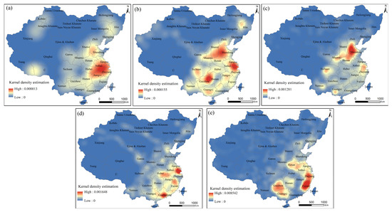
Figure 2.
KDE Distributions of Different Types of Settlements. (a) represents SC1−level settlements; (b) represents SC2; (c) represents SC3; (d) represents SC4; and (e) represents SC5.
SC1 (provincial level, Figure 2a) is concentrated in the Yangtze River Delta, while forming a secondary dense belt in the North China Plain. Henan—Shandong—Zhejiang—Anhui constitute the core agglomeration area. The Mongolian Plateau exhibits a typical low-low agglomeration area. As China’s economic core region since the Song Dynasty, the Yangtze River Delta aggregates the highest hierarchical settlement clusters (Figure 3a).
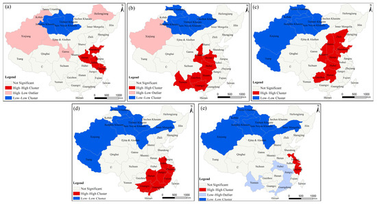
Figure 3.
Local Moran’s I Cluster Analysis Results for Different Types of Settlements. (a) represents SC1−level settlements; (b) represents SC2; (c) represents SC3; (d) represents SC4; and (e) represents SC5.
SC2 (prefectural level, Figure 2b) is primarily distributed in the middle and lower reaches of the Yellow River, the Yangtze River Delta, the Sichuan Basin, and the Yunnan-Guizhou Plateau. The provinces and regions exhibiting high-high agglomeration areas form an arc-shaped belt oriented from northeast to southwest, extending from Shaanxi to Yunnan, thereby presenting a typical central corridor pattern (Figure 3b). This distribution reflects the pivotal role of prefectural seats within the regional administrative network.
SC3 (county-level, Figure 2c) is primarily concentrated in the North China Plain, Sichuan Basin, and Yangtze River Delta. According to the Local Moran results (Figure 3c), its agglomeration centers exhibit high overlap with the secondary settlement provinces and regions, forming a northeast-southwest orientation from Zhili to Guizhou. This pattern underscores the hierarchical interconnectivity between prefectures and counties. SC4 (towns and postal stations, Figure 2d) more prominently reflects economic functions, with distributions centered in the Yangtze River Delta, Pearl River Delta, middle reaches of the Yangtze River basin, and Fujian coastal areas. In China’s southeastern coastal provinces and regions, it displays typical high-high agglomeration, whereas the northwestern regions feature sparse distributions, forming low-low clusters (Figure 3d).
SC5 (village-level, Figure 2e) is primarily concentrated in eastern China, particularly along the southeastern coast, southwestern regions, and the provinces and regions in the middle and lower reaches of the Yellow River, demonstrating the characteristic that provinces with larger map scales have more detailed records. According to the Local Moran analysis (Figure 3e), it still exhibits a high-high zone centered on the Yangtze River Delta, while the northwestern regions form a low-low zone, reflecting spatial disparities in economic development.
3.2. Settlement Clustering Characteristics
To elucidate the spatial agglomeration characteristics of settlements in mainland China at the end of the Qing Dynasty (as reflected in the mapped areas), this study employs the Average Nearest Neighbor Index (NNR) and Moran’s I spatial autocorrelation to analyze settlements of different settlement hierarchies, respectively.
The results indicate that the NNR values for settlements of different hierarchical levels differ significantly (Table 1). For SC1, the NNR is 1.2054, with a Z value of 2.0037 and a significance level of p < 0.05, suggesting that provincial capitals exhibit a slightly dispersed distribution nationwide, primarily due to the limited number of provincial capitals and their adherence to administrative division regulations. In contrast, SC2 (NNR = 0.7838), SC3 (NNR = 0.7474), SC4 (NNR = 0.5513), and SC5 (NNR = 0.6124) all demonstrate significant clustered distributions, with the NNR values decreasing and the clustering intensity strengthening as the hierarchical level declines. Notably, SC4 and SC5 exhibit Z values of −34.5313 and −71.1171, respectively, underscoring their highly concentrated distributions and reflecting the strong dependence of grassroots settlements on natural environments and transportation networks. Although the NNR value of SC5 (villages) is slightly higher than that of SC4 (towns), this pattern reflects the broader spatial spacing of agricultural villages rather than a data artifact. As noted by Zhao, historical Chinese settlements exhibited a hierarchical differentiation in which large villages gradually evolved into towns (“ju cun wei zhen,” 巨村为镇, meaning “large villages becoming towns”) [29]. Villages were constrained by arable land availability and terrain conditions, whereas towns were more concentrated along transportation corridors and trade nodes, leading to a relatively tighter clustering pattern.

Table 1.
NNR Analysis Results.
The Moran’s I index further validates this trend (Table 2). The Moran’s I values are 0.3818 for SC1, 0.3686 for SC2, 0.5548 for SC3, 0.5900 for SC4, and 0.3637 for SC5, all significant at the 1% level. This indicates that all five hierarchical levels of settlements exhibit overall spatial positive autocorrelation, manifesting as a clustered pattern characterized by “like neighbors like.” Among them, SC3 and SC4 exhibit the highest Moran’s I values, demonstrating the strongest spatial clustering and suggesting that, within the late Qing settlement system, the spatial organization at the county- and town-levels was the most compact.
Table 2.
Spatial autocorrelation index Analysis Results.
In summary, this study draws the following conclusions: the settlement system at the end of the Qing Dynasty exhibits a significant spatial distribution characteristic of “high hierarchical levels being relatively dispersed and low hierarchical levels being highly clustered.” The distributions of provincial and prefectural cities are predominantly influenced by administrative division policies, whereas counties, towns, and villages demonstrate evident spatial self-organization features, which are closely associated with resource accessibility, transportation convenience, and population carrying capacity in the context of an agricultural society.
3.3. Hierarchical Structure and Rank-Size Analysis
In terms of quantity indicators, the slopes for the number of settlements in SC2–SC4 range from q ≈ 2.52–3.67, while R2 values are generally low (<0.22) (Figure 4). The steep slopes indicate a pronounced hierarchical gradient, reflecting strong primacy and concentration of higher-level settlements in a few dominant provinces. However, the low R2 values reveal weak internal continuity and poor hierarchical coherence, suggesting that the middle- and upper-level settlement systems were fragmented rather than smoothly ordered. In other words, although the hierarchy was steep, the internal structure lacked stability and completeness across provinces.
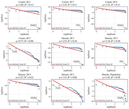
Figure 4.
Rank-Size Results for Settlements Based by Province. Outer Mongolia was excluded from the Rank-Size Analysis. For provinces with zero counts (e.g., Qinghai and Tibet at certain levels), a small constant (10−12) replaced zeros to allow logarithmic transformation without impacting rank order or model stability.
For SC5, the slope is q = 0.77 with R2 = 0.86, showing a good power-law fit (Figure 4). This indicates a flatter rank-size curve and a more even distribution of numerous small settlements, rather than a strict adherence to Zipf’s law (q ≈ 1). The pattern suggests that grassroots settlements formed a more continuous and spatially balanced system, highlighting the overall regularity and completeness of the settlement network in densely populated regions.
In terms of density indicators, the q values for SC2–SC4 are approximately 2.27–2.53, with low R2 values (0.18–0.22) (Figure 4), indicating substantial spatial density variations among mid- to high-level settlements and strong regional unevenness. In contrast, SC5 (q = 1.33, R2 = 0.80) and population density (q = 1.63, R2 = 0.58) exhibit better power-law fits (Figure 4). At the national scale, population distribution adheres to a stronger power-law regularity.
In summary, the Rank-Size analysis reveals that the high-level (SC2–SC3) and SC4 settlement systems are imperfect, characterized by severe hierarchical fractures and regional unevenness. In contrast, the grassroots settlement (SC5) system is relatively complete, with its distribution more closely conforming to Zipf’s law. Provincial population distributions also largely adhere to Zipf’s law, with the corresponding Rank-Size slope for settlement populations being q = 1.14 and R2 = 0.60, approaching the classic Zipf’s law (q ≈ 1). This indicates a tendency toward regularization in the spatial densities of grassroots settlements and population distributions. It further underscores the supportive role of population dynamics in the hierarchization of the settlement system. Overall, these findings elucidate the “duality” of the late Qing Chinese settlement system: imbalance in the upper hierarchies, juxtaposed against a vast and highly regular grassroots structure.
3.4. Influencing Factors of Settlement Hierarchical Distribution
3.4.1. Relationship Between Settlement Hierarchy and Environmental Factors
From the statistical results and box plot comparisons of settlement levels and environmental factors, settlements of different hierarchical levels exhibit certain regular differences in terms of distance to rivers, distance to roads, slope, and elevation (Figure 5).
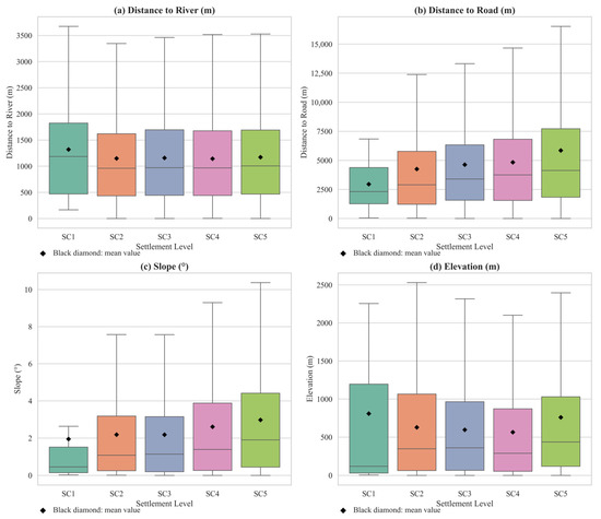
Figure 5.
Relationships between Various Settlement Types and Environmental Factors: (a) River Distance, (b) Road Distance, (c) Slope, and (d) Elevation.
1. River Distance The average distances of settlements at various levels to rivers are roughly between 1100 and 1300 m, with no significant differences. The box plots show that the distributions for the five levels are relatively similar, with medians maintained at around 1 km. This indicates that whether settlements are provincial cities, prefectural cities, or grassroots settlements, they all tend to be built along rivers, making rivers a common factor in site selection for settlements of different levels in the early 20th century.
2. Road Distance There are significant differences in road accessibility among different hierarchical levels of settlements. SC1 averages about 3 km from roads, with prefectural and county-level settlements gradually increasing, and SC5 having the highest average distance to roads, reaching 5–6 km. The box plots show that as the level decreases, the mean and median of the distribution overall rise, indicating that higher-level settlements are closer to major transportation routes. This aligns with the functions of provincial and prefectural cities as transportation hubs and administrative centers in the late Qing Dynasty.
3. Slope The lower the settlement level, the greater the slope at its site. The medians for SC1 and SC2 are both below 2°, indicating that high-level settlements are mostly distributed in plains or basins with gentle terrain; meanwhile, for SC5, the median is close to 2°, the 75th percentile is near 4.5°, and some even exceed 20°, reflecting that grassroots settlements are more distributed in hilly and mountainous areas.
4. Elevation Differences in elevation among different levels of settlements are relatively obvious. SC1 has an average elevation of about 800 m, with a wide distribution range; meanwhile, SC3 and SC4 have medians generally below 400 m; SC5, although with an average elevation of about 760 m, has a large distribution span, with some villages located in the Tibetan Plateau region above 6000 m. Overall, high-level settlements are more concentrated in mid-to-low elevation plains and basins, while low-level settlements are more dispersed, including more mountainous samples (Figure 6).
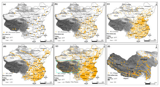
Figure 6.
Spatial Overlay Visualization of Settlements at Different Levels and Elevation. (a) represents SC1−level settlements; (b) represents SC2; (c) represents SC3; (d) represents SC4; and (e) represents SC5; (f) represents the settlement distribution on the Qinghai–Tibet Plateau.
Overall, high-level settlements (provincial SC1, prefectural SC2) exhibit greater dependence on areas with convenient transportation and gentle terrain for site selection, whereas mid- to low-level settlements (towns SC4, villages SC5) demonstrate stronger terrain adaptability, with broader distribution ranges and particularly higher proportions in high-elevation and mountainous regions (Figure 6). This underscores the significant coupling relationship between the settlement hierarchy and the natural environment in late Qing China: high-level settlements leverage rivers, roads, and plains to perform administrative and economic core functions, while low-level settlements more prominently reflect the survival and adaptation of human habitations amid complex natural terrains.
3.4.2. Differences and Driving Factors Between Settlement Hierarchy and Environmental Factors
The results of one-way ANOVA indicate that settlements of different hierarchical levels exhibit significant differences in road distance (F = 18.85, p < 0.001), slope (F = 23.87, p < 0.001), and elevation (F = 22.29, p < 0.001), whereas the differences in river distance are not significant (F = 0.58, p = 0.676) (Table 3).
Table 3.
One-way ANOVA and Tukey HSD results for environmental factors across settlement hierarchies.
Further Tukey’s HSD post hoc multiple comparisons reveal (Table 3): (1) In terms of road distance, SC5 differs significantly from SC2–SC4, reflecting that low-level settlements are farther from major transportation trunk lines; (2) In terms of slope, SC5 exhibits significant differences from all other levels, indicating that villages are more frequently distributed in hilly areas with steeper slopes; (3) In terms of elevation, the distribution of SC5 is significantly higher than that of SC3 and SC4, suggesting stronger adaptability of villages to high-elevation terrains; (4) River distance shows no significant differences among levels, indicating that river-dependent siting is a universal feature of settlements, without manifesting hierarchical distinctions.
To further elucidate the influence of environmental factors on settlement hierarchy, this study constructed an ordered logistic regression model, the results of which validate this trend: road distance (coef = 3.12 × 10⁻⁵, p < 0.001), slope (coef = 0.044, p < 0.001), and elevation (coef = 0.0001, p < 0.001) all exert significant positive effects on settlement hierarchy, while river distance remains insignificant (Appendix C). This indicates that the hierarchical structure of the settlement system in late Qing China is primarily constrained by transportation accessibility and terrain conditions, with high-level settlements concentrated in regions featuring convenient transportation and gentle topography, whereas low-level settlements are more extensively distributed in mountainous and plateau areas.
3.5. Evaluation of Map Scale Effects on Settlement
The varying scales of sub-maps in the Complete Map of the Great Qing Empire may introduce spatial bias in settlement extraction, particularly for low-level settlements (SC5), which are more sensitive to mapping detail. Due to the SC5 in the Qinghai-Tibet Plateau and Mongolian Plateau being mostly drawn along roads, they were not included in the analysis.
To evaluate this effect, regression and visualization analyses were performed using ln(SC5) as the dependent variable and six explanatory factors: ln(Scale), ln(Estimated Settlements_1930s), ln(Household_1912), ln(Cropland_1908), ln(Mean Elevation), and ln(Mean Slope).
Scatterplots revealed that Fujian, Guizhou, and Guangxi were distinct outliers, with abnormally high SC5 values relative to their scales (Figure 7). Across all provinces, ln(Scale) and ln(SC5) show a significant negative relationship (R2 = 0.36, p < 0.01), indicating that smaller-scale maps tend to contain fewer recorded villages. Household also shows a positive correlation (R2 = 0.20, p < 0.05), while other factors were not significant.
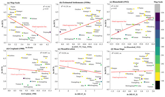
Figure 7.
Scale-bias visualization across all provinces. Scatterplots showing the relationships between village−level settlements (ln SC5) and six explanatory variables: (a) Map Scale, (b) Estimated Settlements (1930s), (c) Household 1912, (d) Cropland 1908, (e) Mean Elevation, and (f) Mean Slope.
When the three outlier provinces were excluded, the correlations strengthened markedly (Figure 8): Scale–SC5 (R2 = 0.27, p < 0.05), Estimated Settlements 1930s–SC5 (R2 = 0.27, p < 0.05), Household–SC5 (R2 = 0.41, p < 0.01), and Cropland–SC5 (R2 = 0.30, p < 0.05). This confirms that extreme scale deviations concentrated in a few provinces may distort national patterns.
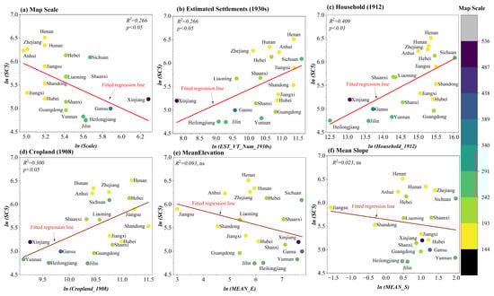
Figure 8.
Scale−bias visualization excluding Fujian, Guizhou, and Guangxi. Same as Figure 7 but with three provinces (Fujian, Guizhou, Guangxi) removed. Scatterplots showing the relationships between village−level settlements (ln_SC5) and six explanatory variables: (a) Map Scale, (b) Estimated Settlements (1930s), (c) Household 1912, (d) Cropland 1908, (e) Mean Elevation, and (f) Mean Slope.
Multiple regression analysis (Table 4) using ln(Scale), ln(Household_1912), ln(Cropland_1908), ln(Mean Elevation), and ln(Range Slope) further validates this pattern. For the full sample (N = 22), the model shows R2 = 0.52 (Adj. R2 = 0.37, F = 3.49, p = 0.025), with a negative but statistically weak coefficient for Scale (–0.81, p = 0.16). After excluding the three provinces (Table 5) (N = 19), R2 = 0.43 (Adj. R2 = 0.21, p = 0.15), and the Scale coefficient diminishes (–0.34, p = 0.59). Thus, map scale effects are primarily localized rather than systemic, and removing the outliers does not substantially alter the national model (ΔR2 < 0.1).
Table 4.
Regression results for ln (SC5)—full sample.
Table 5.
Regression results for ln (SC5)—excluding Fujian, Guizhou, and Guangxi.
Overall, these results suggest that map scale correlates with spatial variation in SC5 but acts more as a derivative indicator linked to topographic complexity and socioeconomic conditions rather than an independent driver. Consequently, while scale bias exists, it does not significantly distort the national-level conclusions on settlement hierarchies. The detailed regression coefficients and statistics are provided in Table 4 and Table 5 and Appendix D. For clarity, Table 4 and Table 5 summarize the results for the full and reduced samples, while additional models examining the determinants of map scale and household distribution are reported in the Appendix D.
4. Discussion
This section discusses how the empirical results address the study’s main questions regarding the spatial distribution, hierarchical structure, and environmental determinants of settlements in late Qing China.
4.1. Causes of Formation of Settlement Distribution Patterns
This study indicates that by the end of the Qing Dynasty (late 19th to early 20th century), the Chinese settlement system had evolved to a critical period of social transformation marked by increasingly close connections between China and the world [30]. The spatial pattern of the national settlement system exhibits the following characteristics: high-level settlements are distributed relatively dispersed, whereas mid-to low-level settlements demonstrate high clustering. This disparity primarily stems from three aspects:
First, the establishment of high-level settlements such as provinces and prefectures adheres to the distribution pattern of national administrative divisions, placing greater emphasis on spatial equilibrium in political jurisdiction rather than optimal selections based on economic and natural conditions. This aligns closely with the insights from studies on Chinese historical political geography. Existing research indicates that “mountains and rivers convenient” (shanchuan xingsheng, 山川形胜) and “interlocking teeth” (quanyan jiaocuo, 犬牙交错) constituted the two major principles of administrative divisions during historical periods in China. The former delineates administrative divisions based on natural geographical conditions, yet geomorphic areas such as basins are prone to fostering local decentralization that opposes central authority [31]. Consequently, “artificial administrative divisions” (such as the multiple provinces of the Yuan Dynasty) that span multiple natural geomorphic areas and are dominated by central power emerged as necessary choices [31]. Therefore, the settlement system in China at the turn of the 20th century can also be interpreted from the perspective of spatial power.
Second, low-level settlements are more dependent on natural environments and transportation conditions, particularly the constraining effects of road accessibility, terrain slope, and elevation, which give rise to evident self-organizing clustering phenomena in social behaviors and economic activities. This aligns with G. William Skinner’s interpretation of the traditional Chinese settlement system, integrating Christaller’s Central Place Theory [13,32]. Furthermore, transportation networks represent a crucial aspect of China’s national spatial organizational capacity during historical periods (including the transmission of information and the transfer of materials [33]), while the importance of rivers has relatively declined. This also explains why river distance did not exhibit significance in the statistical tests of this study.
4.2. Explanation of Settlement Hierarchical Differences
Through the systematic digitization of the Complete Map of the Great Qing Empire, this study reveals, at the national scale, the coexistence of hierarchical fractures and underlying regularities within the settlement system. On one hand, Rank-Size analysis indicates that the mid- to high-level settlement system is imperfect, lacking an ideal power-law distribution and exhibiting a pronounced “fractured” pattern, which is largely attributable to the spatial operations of political power. On the other hand, low-level settlements and population distributions more closely conform to Zipf’s law, reflecting the universality and orderliness of the underlying network. These findings suggest that during the social transformation process in modern China, the administratively dominated upper hierarchy displayed imbalance and vulnerability, whereas the grassroots settlement network played a more enduring role in sustaining social operations and population carrying capacity.
Christaller proposed the Central Place Theory in the early twentieth century (1933) [32], which emphasizes that settlements of different hierarchical levels form a spatially ordered system based on service capacity and market range. The case of early-twentieth-century China illustrates a comparable pattern: higher-order settlements such as provincial and prefectural centers functioned as major central places, offering diversified services over broader areas; meanwhile, lower-order settlements, such as villages, served as minor central places with limited functions, smaller service radii, and denser distributions. The location and spacing of these centers were essentially determined by their threshold and range.
In late Qing China, higher-level settlements (SC1–SC3) were concentrated at administrative and transportation nodes, performing regional coordination and market functions analogous to Christaller’s higher-order centers. In contrast, lower-level settlements (SC4–SC5) exhibited a more uniform and spatially continuous pattern, providing localized services within agrarian landscapes.
However, the observed hierarchy also departs from the idealized hexagonal regularity envisioned by Christaller. The steep rank-size slopes (high q values) and fragmented mid-level structures reveal the influence of administrative boundaries, topographic constraints, and agrarian production systems, which shaped a state-regulated rather than purely market-driven central-place network. This indicates that the Qing settlement hierarchy embodied both functional centrality and territorial governance, adapting central-place logic to a national social-economic and political context.
Furthermore, the various cartographic elements, including the scale, also embody hierarchy. Text, image, and the construction of regional knowledge are essential components of Humanistic Geography. As Buttime argues, humanistic geography concerns not only how people interpret their everyday “lifeworlds,” but also how academic and cartographic representations project particular “mindscapes” [34]. In this sense, the variations in map scale observed in this study also reflect deeper socio-economic and geographical factors, particularly their dependence on provincial area and administrative delineation. The provincial maps of the Complete Map of the Great Qing Empire thus function as visual confirmations of the political spatialization of power, where the delineation of provinces and counties represents a human-constructed geography deeply embedded in administrative and cultural logics.
4.3. Limitations and Prospects
It should be noted that this study still has several limitations. First, the Complete Map of the Great Qing Empire features varying scales across its sub-maps, with some regions (such as the Tibetan Plateau and northwestern frontiers) exhibiting missing place names or uncertain boundaries, potentially leading to uneven settlement data. Second, the research primarily relies on natural environmental and transportation factors, without incorporating the socio-economic, social, and institutional factors prevalent at the time. Future studies could introduce richer multi-source historical geographic data (such as population censuses and railway transportation records) for comprehensive analysis, thereby further deepening the interpretation of the causal mechanisms underlying settlement patterns. Additionally, systematic application of spatial georeferencing and error correction methods in future research would enhance data precision and the reliability of results.
Although the map-scale heterogeneity among sub-maps inevitably introduces minor regional bias—particularly in southwestern provinces—our regression analysis (Section 3.5) shows that such bias has limited statistical significance after excluding extreme cases. Therefore, while scale differences should be acknowledged as a data limitation, they do not systematically alter the main spatial or hierarchical conclusions of this study.
5. Conclusions
Overall, these findings directly address the research questions outlined in the Introduction and extend both theoretical and empirical understandings of settlement hierarchy and human–land interaction in historical China.
Utilizing digitized data from the Complete Map of the Great Qing Empire (1905), this study systematically reconstructs and analyzes the spatial structure and formative mechanisms of the settlement system in mainland China at the end of the Qing Dynasty. The main conclusions are as follows:
1. The late Qing settlement system displays a typical dual structure—relatively dispersed high-level settlements and highly clustered low-level ones—reflecting the combined effects of administrative division and environmental–transportation conditions.
2. Rank–Size analysis reveals pronounced hierarchical steepness and regional unevenness among mid- to high-level settlements, whereas the grassroots system exhibits a more even and continuous pattern approximating Zipf’s law.
3. Statistical analyses identify transportation accessibility, slope, and elevation as major determinants of settlement hierarchy, while river proximity plays a minor role. These results suggest that the organization of settlements in late Qing China was primarily shaped by transportation connectivity and terrain adaptability.
In summary, the late Qing settlement system embodied a clear duality: the administratively dominated upper hierarchy was fragmented and vulnerable, whereas the self-organizing grassroots network was extensive and resilient.
By bridging spatial–statistical analysis with historical cartography, this study not only reconstructs the macro-scale structure of China’s pre-modern settlements but also extends central-place and humanistic perspectives to an imperial agrarian context. It thus contributes to the broader field of land science by demonstrating how digitized historical maps can serve as quantitative evidence for exploring long-term human–land systems and the spatial evolution of socio-environmental organization.
Author Contributions
Conceptualization, R.S. and Z.Z.; methodology, R.S. and Z.Z.; software, R.S.; validation, R.S. and Z.Z.; formal analysis, R.S.; investigation, R.S. and Z.Z.; resources, R.S. and Z.Z.; data curation, R.S.; writing—original draft preparation, R.S.; writing—review and editing, Z.Z.; visualization, R.S.; supervision, Z.Z.; project administration, R.S. and Z.Z.; funding acquisition, R.S. and Z.Z. All authors have read and agreed to the published version of the manuscript.
Funding
This research has been funded by the major project program of the National Social Science Fund of China, grant number 20&ZD230. The work was also funded by the Postdoctoral Research Project of Guangzhou Municipality (625136-07).
Data Availability Statement
The associated data set in the study is available upon request.
Acknowledgments
The authors gratefully acknowledge the constructive feedback from the anonymous reviewers and the helpful guidance from the Academic Editor, which significantly contributed to improving this manuscript.
Conflicts of Interest
The authors declare no conflicts of interest.
Appendix A
This study is based on the basic information of each map sheet in the atlas. Different levels of settlements were digitized and extracted in ArcGIS 10.8, and the areas of provincial-level administrative units were calculated. At the same time, the scales of the different map sheets, as well as the control points for each map sheet during registration along with RMS error and Transformation Order, were recorded.
Table A1.
RMSE and Georeferencing Accuracy Summary.
Table A1.
RMSE and Georeferencing Accuracy Summary.
| Province | Transformation Order | Ground Control Points | Total RMS Error |
|---|---|---|---|
| Zhili | 2 | 21 | 0.00751812 |
| Shengjing | 2 | 9 | 0.00377645 |
| Jilin | 2 | 7 | 0.002 |
| Heilongjiang | 3 | 10 | 3.26 × 10⁻¹² |
| Shandong | 2 | 9 | 0.00297079 |
| Shanxi | 2 | 10 | 0.00623676 |
| Henan | 3 | 11 | 0.00277099 |
| Jiangsu | 3 | 13 | 0.00246838 |
| Anhui | 3 | 14 | 0.00228901 |
| Jiangxi | 3 | 17 | 0.00271372 |
| Fujian | 3 | 20 | 0.00277796 |
| Zhejiang | 3 | 24 | 0.00244408 |
| Hubei | 2 | 26 | 0.00747131 |
| Hunan | 2 | 31 | 0.00577058 |
| Shaanxi | 2 | 31 | 0.00688398 |
| Gansu | 2 | 23 | 0.0106866 |
| Xinjiang | 3 | 16 | 0.011003 |
| Sihuan | 3 | 16 | 0.00594714 |
| Guangdong | 3 | 13 | 0.00304336 |
| Guangxi | 3 | 13 | 0.00328411 |
| Yunnan | 3 | 15 | 0.00769711 |
| Guizhou | 3 | 11 | 0.00188859 |
| Inner Mongolia and Outer Mongolia | 3 | 10 | 2.26 × 10⁻¹² |
| Qinghai and Tibet | 3 | 17 | 0.0138929 |
| County | 3 | 21 | 0.0618996 |
Table A2.
Basic Information of Each Map Sheet.
Table A2.
Basic Information of Each Map Sheet.
| Province | SC5 | SC4 | SC3 | SC2 | SC1 | Scale (×10,000) | Area/km2 |
|---|---|---|---|---|---|---|---|
| Jiangsu | 365 | 90 | 50 | 12 | 2 | 180 | 102,494.4435 |
| Anhui | 510 | 87 | 46 | 10 | 1 | 144 | 149,050.1794 |
| Zhejiang | 526 | 50 | 56 | 7 | 1 | 150 | 93,384.8759 |
| Jiangxi | 207 | 107 | 64 | 13 | 1 | 150 | 183,326.3604 |
| Hunan | 569 | 90 | 57 | 13 | 1 | 180 | 216,480.976 |
| Hubei | 183 | 119 | 58 | 11 | 1 | 180 | 187,872.6896 |
| Fujian | 862 | 103 | 46 | 8 | 1 | 150 | 122,891.2128 |
| Guangdong | 143 | 163 | 62 | 15 | 1 | 225 | 210,036.9283 |
| Guangxi | 695 | 99 | 74 | 14 | 1 | 180 | 210,664.7611 |
| Yunnan | 125 | 75 | 70 | 15 | 1 | 270 | 353,762.7998 |
| Guizhou | 806 | 40 | 49 | 18 | 1 | 150 | 177,312.9463 |
| Sichuan | 442 | 66 | 115 | 24 | 1 | 290 | 574,116.7976 |
| Zhili | 461 | 64 | 143 | 19 | 1 | 225 | 326,837.6076 |
| Henan | 673 | 42 | 94 | 11 | 1 | 180 | 182,741.147 |
| Shandong | 253 | 30 | 88 | 11 | 1 | 180 | 135,146.5951 |
| Shanxi | 171 | 50 | 93 | 18 | 1 | 225 | 240,530.1796 |
| Shaanxi | 294 | 34 | 74 | 10 | 1 | 225 | 192,225.9077 |
| Gansu | 148 | 66 | 41 | 14 | 0 | 360 | 465,410.8025 |
| Xinjiang | 181 | 40 | 17 | 15 | 1 | 536 | 1,587,280.443 |
| Liaoning | 291 | 25 | 22 | 3 | 1 | 225 | 158,322.2775 |
| Jilin | 115 | 50 | 14 | 13 | 1 | 277 | 285,886.4389 |
| Heilongjiang | 116 | 13 | 2 | 5 | 1 | 277 | 469,045.0727 |
| Qinghai | 76 | 0 | 2 | 0 | 0 | 500 | 674,112.408 |
| Tibet | 189 | 1 | 0 | 0 | 2 | 500 | 1,042,683.343 |
| Inner Mongolia | 179 | 13 | 29 | 1 | 0 | 720 | 671,899.3172 |
| Outer Mongolia | 317 | 45 | 52 | 4 | 1 | 720 | 2,009,539.735 |
Appendix B. Offset Error Assessment Based on Provincial Administrative Points (SC1)
Based on a comparison between the Complete Map of the Great Qing Empire (1905) and modern geographic coordinates (2020) (National Catalogue Service for Geographical Information, (https://www.webmap.cn/commres.do?method=result100W, accessed on 15 September 2025), this study extracted 25 provincial capital sample points for error verification. The results (Table A2) indicate:
- (1)
- Overall Error Level
The average spatial deviation is 13.82 km, with a standard deviation of approximately 9.16 km. The median error is 12.96 km, suggesting that most provincial capitals have deviations between 10 and 20 km. The minimum error occurs in Guilin (approximately 1.44 km), while the maximum error is observed in Urumqi (approximately 42.90 km).
- (2)
- Error Distribution Characteristics
The Shapiro–Wilk test for normality yields W = 0.898, p = 0.017 < 0.05, indicating that the error distribution significantly deviates from normality. The one-sample t-test results in t = 7.54, p < 0.001, suggesting that the average error is significantly greater than 0, i.e., the map exhibits systematic positional bias.
Table A3.
Offset Error Assessment Based on Provincial Administrative Points (SC1).
Table A3.
Offset Error Assessment Based on Provincial Administrative Points (SC1).
| ID_Name_1905 | X_1905 | Y_1905 | X_2020 | Y_2020 | ΔX | ΔY | Error_Deg | Error_km |
|---|---|---|---|---|---|---|---|---|
| Anqing | 117.0224423 | 30.53577301 | 117.1099265 | 30.53468488 | −0.087484212 | 0.001088137 | 0.087490979 | 8.396228753 |
| Beijing | 116.428851 | 39.89554265 | 116.7184397 | 39.9037508 | −0.289588727 | −0.008208151 | 0.28970503 | 24.78201378 |
| Changsha | 112.7852863 | 28.25089544 | 112.9778777 | 28.1176484 | −0.192591341 | 0.133247045 | 0.234192655 | 23.99364324 |
| Chengdu | 104.0162228 | 30.67543945 | 104.0739775 | 30.65382477 | −0.057754699 | 0.021614672 | 0.061666841 | 6.031477 |
| Fuzhou | 119.4141842 | 26.02749088 | 119.2902992 | 26.10348401 | 0.123884951 | −0.075993129 | 0.1453356 | 14.98494339 |
| Guangzhou | 113.4252021 | 23.12833714 | 113.261191 | 23.13494289 | 0.164011114 | −0.006605752 | 0.164144088 | 16.81440642 |
| Guilin | 110.1880771 | 25.24365196 | 110.175127 | 25.238142 | 0.012950135 | 0.005509957 | 0.014073579 | 1.44046739 |
| Guiyang | 106.556203 | 26.53360341 | 106.701798 | 26.603715 | −0.14559501 | −0.070111588 | 0.161596849 | 16.45480218 |
| Hangzhou | 120.0852292 | 30.28499581 | 120.148136 | 30.26970368 | −0.06290674 | 0.015292135 | 0.064738762 | 6.285609116 |
| Jilin | 126.8578992 | 43.75287698 | 126.5434374 | 43.83580482 | 0.314461856 | −0.082927842 | 0.325212678 | 26.93378201 |
| Jinan | 116.948567 | 36.60572913 | 117.0152951 | 36.66950549 | −0.066728028 | −0.063776362 | 0.092304139 | 9.257492083 |
| Kaifeng | 114.466899 | 34.92684577 | 114.3017044 | 34.79879922 | 0.165194595 | 0.128046551 | 0.209009984 | 20.7355411 |
| Kunming | 102.8314418 | 25.10092784 | 102.7087542 | 25.04927972 | 0.122687594 | 0.051648116 | 0.13311564 | 13.63607103 |
| Lanzhou | 103.8521813 | 36.13957498 | 103.8239565 | 36.06137196 | 0.028224822 | 0.078203018 | 0.083140559 | 9.042035328 |
| Lhasa | 91.01862424 | 29.68747549 | 91.115889 | 29.651787 | −0.097264764 | 0.035688492 | 0.103605515 | 10.21293029 |
| Nanchang | 115.8130994 | 28.56999339 | 115.8081269 | 28.6411754 | 0.004972427 | −0.07118201 | 0.071355473 | 7.904027636 |
| Nanjing | 118.7805656 | 32.06052635 | 118.7579787 | 32.06376979 | 0.0225869 | −0.003243443 | 0.022818588 | 2.162977744 |
| Qiqihar | 123.8271074 | 47.19768643 | 123.9115462 | 47.35251839 | −0.084438809 | −0.154831959 | 0.176359995 | 18.36106655 |
| Shenyang | 123.4987109 | 41.85937562 | 123.4252886 | 41.8337045 | 0.073422303 | 0.025671125 | 0.077780725 | 6.73139648 |
| Shigatse | 88.72011203 | 29.25381927 | 88.87854907 | 29.2704495 | −0.158437037 | −0.016630221 | 0.159307435 | 15.50875132 |
| Suzhou | 120.5211469 | 31.29703707 | 120.5811607 | 31.30120784 | −0.060013776 | −0.004170769 | 0.060158529 | 5.732285544 |
| Taiyuan | 112.5033247 | 37.91656901 | 112.572592 | 37.81352301 | −0.069267227 | 0.103046 | 0.124162904 | 12.96014929 |
| Ürümqi | 87.52520206 | 43.41263797 | 87.62580371 | 43.79177926 | −0.100601652 | −0.379141294 | 0.392261155 | 42.90025457 |
| Wuhan | 114.1657855 | 30.55402568 | 114.3361849 | 30.54883684 | −0.170399406 | 0.005188844 | 0.170478391 | 16.35966227 |
| Xi’an | 108.8632998 | 34.26565175 | 108.9495464 | 34.26709703 | −0.086246662 | −0.00145287 | 0.086258771 | 7.94453985 |
Box plots and histograms further illustrate that the overall errors are concentrated between 10 and 20 km, but certain cities (such as Urumqi, Lhasa, Beijing, and Jilin) represent outlier deviation points.

Figure A1.
Histogram of Geographic Error Distribution for Provincial Settlements (SC1).

Figure A2.
Box Plot of Geographic Error Distribution for Provincial Settlements (SC1).
- (3)
- Geographic Differences
Inland provincial capitals (such as Nanjing, Hangzhou, and Chengdu) generally exhibit lower errors (<10 km), reflecting higher cartographic accuracy in the Yangtze River Basin and North China Plain regions.
Frontier and western provincial capitals (such as Urumqi, Lhasa, Kunming, and Guiyang) show relatively larger errors, indicating that mapping conditions in frontier areas during the late Qing Dynasty were limited, leading to reduced positional accuracy.
Appendix C. Detailed Results of the Ordered Logistic Regression Model for Settlement Hierarchy
Table A4.
Ordered Logistic Regression Results for Environmental Determinants of Settlement Hierarchy.
Table A4.
Ordered Logistic Regression Results for Environmental Determinants of Settlement Hierarchy.
| Variable | coef | std err | z | p > |z| | [0.025 | 0.975] |
|---|---|---|---|---|---|---|
| NEAR_DIST (River) | −1.066 × 10⁻⁵ | 2.31 × 10⁻⁵ | −0.461 | 0.645 | −5.6 × 10⁻⁵ | 3.47 × 10⁻⁵ |
| NEAR_DIST (Road) | 3.118 × 10⁻⁵ | 4.38 × 10⁻⁶ | 7.118 | 0.000 | 2.26 × 10⁻⁵ | 3.98 × 10⁻⁵ |
| SlopeGDEMM | 0.0441 | 0.008 | 5.624 | 0.000 | 0.029 | 0.060 |
| GDEMM2024 (Elevation) | 0.0001 | 2.91 × 10⁻⁵ | 3.641 | 0.000 | 4.9 × 10⁻⁵ | 0.000 |
| /cut1 | −5.8197 | 0.199 | −29.193 | 0.000 | −6.210 | −5.429 |
| /cut2 | 0.9139 | 0.075 | 12.119 | 0.000 | 0.766 | 1.062 |
| /cut3 | 0.6172 | 0.029 | 21.487 | 0.000 | 0.561 | 0.673 |
| /cut4 | −0.2173 | 0.025 | −8.857 | 0.000 | −0.265 | −0.169 |
The ordered logistic regression model assesses the impact of environmental factors on settlement hierarchy (SC1–SC5 as the ordinal dependent variable), assuming proportional odds. Predictors include river distance (NEAR_DIST), road distance (NEAR_DIST), slope (SlopeGDEMM), and elevation (GDEMM2024), with positive coefficients indicating higher hierarchy for greater values (e.g., longer road distances). Cut points (/cut1 to /cut4) denote thresholds between levels. All variables showed low multicollinearity (VIF < 5). Model fitted using statsmodels in Python 3.13.5.
It should be noted that the settlement hierarchy (SC1–SC5) was coded in ascending order (i.e., larger numerical values represent lower hierarchical levels). Therefore, the positive coefficient of “NEAR_DIST (Road)” in the ordered logistic regression does not indicate that higher-level settlements are farther from roads. Instead, it means that as the distance to roads increases, the probability of a settlement belonging to a lower-level category (e.g., SC4–SC5) increases. This finding is consistent with the ANOVA and boxplot results (Figure 6b), which show that higher-level settlements are closer to roads, while lower-level ones tend to be farther away.
Appendix D
To examine the effects of socio-economic and topographic factors on the variation in cartographic scales among provinces, multiple linear regression analyses were conducted with the logarithm of map scale (ln_Scale) as the dependent variable. The explanatory variables include population (ln_Household_1912), cropland area in 1908 (ln_Cropland_1908), mean elevation (ln_MEAN_E), slope range (ln_RANGE_S), and provincial area (ln_Area).
Results indicate that the model is statistically significant (R2 = 0.865, adjusted R2 = 0.823, F = 20.58, p < 0.001), suggesting that these factors collectively explain most of the interprovincial variation in map scale. Among the predictors, ln_Area has the strongest and most significant positive effect (β = 0.432, p < 0.001), implying that provinces with larger spatial extents tend to have maps drawn at larger scales. Socio-economic and terrain factors show the expected directions but are not statistically significant at the national level, reflecting their relatively weaker influence compared with administrative spatial extent.
Table A5.
Regression results for ln (Scale).
Table A5.
Regression results for ln (Scale).
| Coefficients | Std. Error | t-Statistic | p-Value | Lower 95% | Upper 95% | |
|---|---|---|---|---|---|---|
| Intercept | 0.46456 | 1.167902 | 0.397773 | 0.696054 | −2.01128 | 2.940401 |
| ln(Household_1912) | −0.07894 | 0.057072 | −1.38309 | 0.185634 | −0.19992 | 0.042051 |
| ln(Cropland_1908) | 0.086875 | 0.04991 | 1.740608 | 0.100945 | −0.01893 | 0.19268 |
| ln(MEAN_E) | 0.039111 | 0.056498 | 0.692257 | 0.498701 | −0.08066 | 0.158881 |
| ln(RANGE_S) | −0.12928 | 0.158732 | −0.81448 | 0.427325 | −0.46578 | 0.207212 |
| ln(Area) | 0.431831 | 0.075592 | 5.712676 | 3.21 × 10⁻⁵ | 0.271584 | 0.592079 |
Multiple R = 0.9303, R2 = 0.88655, Adj. R2 = 0.8234, F = 20.5844, p = 1.87544 × 10⁻⁶, N = 22.
Table A6.
Regression results for ln (Area).
Table A6.
Regression results for ln (Area).
| Coefficients | Std. Error | t-Statistic | p-Value | Lower 95% | Upper 95% | |
|---|---|---|---|---|---|---|
| Intercept | 12.71729 | 2.127919 | 5.976396 | 0.000015 | 8.227771 | 17.20681 |
| ln(Household_1912) | −0.38826 | 0.157047 | −2.47227 | 0.024286 | −0.7196 | −0.05692 |
| ln(Cropland_1908) | 0.230662 | 0.150048 | 1.53726 | 0.142633 | −0.08591 | 0.547235 |
| ln(MEAN_E) | 0.221663 | 0.173117 | 1.28042 | 0.217593 | −0.14358 | 0.586908 |
| ln(RANGE_S) | 0.501207 | 0.494569 | 1.013421 | 0.325067 | −0.54224 | 1.544657 |
Multiple R = 0.7863, R2 = 0.66183, Adj. R2 = 0.5284, F = 6.8830, p = 0.0017, N = 22.
Table A7.
Regression results for ln (Household).
Table A7.
Regression results for ln (Household).
| Coefficients | Std. Error | t-Statistic | p-Value | Lower 95% | Upper 95% | |
|---|---|---|---|---|---|---|
| Intercept | 13.85549 | 1.481152 | 9.354537 | 1.52 × 10⁻⁸ | 10.75541 | 16.95558 |
| ln(MEAN_E) | −0.74828 | 0.245076 | −3.05327 | 0.006541 | −1.26123 | −0.23533 |
| ln(RANGE_S) | 1.686002 | 0.746555 | 2.258377 | 0.035877 | 0.123445 | 3.24856 |
Multiple R = 0.5765, R2 = 0.3323, Adj. R2 = 0.2620, F = 4.7285, p = 0.0215, N = 22.
Overall, the regression analyses demonstrate that map-scale variation across provinces primarily reflects structural differences in spatial extent (Area), while socio-economic and topographic factors exert secondary effects. This supports the interpretation that cartographic scale heterogeneity in the Complete Map of the Great Qing Empire arises from both administrative spatial delineation and human cartographic practices, rather than from purely natural or socio-economic causes.
References
- Fisher, J.S.; Mitchelson, R.L. Forces of change in the American settlement pattern. Geogr. Rev. 1981, 71, 298–310. [Google Scholar] [CrossRef]
- McLeman, R.A. Settlement abandonment in the context of global environmental change. Glob. Environ. Chang. 2011, 21, S108–S120. [Google Scholar] [CrossRef]
- Carrión, J.S.; Fuentes, N.; González-Sampériz, P.; Sánchez Quirante, L.; Finlayson, J.C.; Fernández, S.; Andrade, A. Holocene environmental change in a montane region of southern Europe with a long history of human settlement. Quat. Sci. Rev. 2007, 26, 1455–1475. [Google Scholar] [CrossRef]
- Kowalewski, S.A. Regional settlement pattern studies. J. Archaeol. Res. 2008, 16, 225–285. [Google Scholar] [CrossRef]
- Mortensen, B. Change in the settlement pattern and population in the beginning of the historical period. Ägypten Levante 1991, 2, 11–37. [Google Scholar]
- Zhang, Q.; Zhu, C.; Liu, C.-L.; Jiang, T. Environmental change and its impacts on human settlement in the Yangtze Delta, PR China. Catena 2005, 60, 267–277. [Google Scholar] [CrossRef]
- Shennan, S.J. Settlement and social change in central Europe, 3500–1500 BC. J. World Prehist. 1993, 7, 121–161. [Google Scholar] [CrossRef]
- Easterlin, R.A. Population change and farm settlement in the northern United States. J. Econ. Hist. 1976, 36, 45–75. [Google Scholar] [CrossRef]
- Li, Y.; Ye, Y.; Fang, X.; Zheng, X.; Zhao, Z. Settlement expansion influenced by socio-cultural changes in western Hunan mountainous areas of China during the eighteenth century. J. Hist. Geogr. 2022, 78, 22–34. [Google Scholar] [CrossRef]
- Pumain, D. Settlement systems in the evolution. Geogr. Ann. Ser. B Hum. Geogr. 2000, 82, 73–87. [Google Scholar] [CrossRef]
- Artursson, M.; Bech, J.-H.; Earle, T.; Fuköh, D.; Kolb, M.J.; Kristiansen, K.; Ling, J.; Mühlenbock, C.; Prescott, C.; Sevara, C. Settlement structure and organisation. In Organizing Bronze Age Societies: The Mediterranean, Central Europe, and Scandanavia Compared; Earle, T., Kristiansen, K., Eds.; Cambridge University Press: Cambridge, UK, 2010; pp. 87–121. [Google Scholar]
- Bura, S.; Guérin-Pace, F.; Mathian, H.; Pumain, D.; Sanders, L. Multiagent systems and the dynamics of a settlement system. Geogr. Anal. 1996, 28, 161–178. [Google Scholar] [CrossRef]
- Skinner, G.W. Marketing and social structure in rural China, Part I. J. Asian Stud. 1964, 24, 3–43. [Google Scholar] [CrossRef]
- Liu, P.; Zeng, C.; Liu, R. Environmental adaptation of traditional Chinese settlement patterns and its landscape gene mapping. Habitat Int. 2023, 135, 102808. [Google Scholar] [CrossRef]
- Williams, M. “The apple of my eye”: Carl Sauer and historical geography. J. Hist. Geogr. 1983, 9, 1–28. [Google Scholar] [CrossRef]
- Wang, J.; Zhang, Y. Analysis on the evolution of rural settlement pattern and its influencing factors in China from 1995 to 2015. Land 2021, 10, 1137. [Google Scholar] [CrossRef]
- Leyk, S.; Uhl, J.H.; Connor, D.S.; Braswell, A.E.; Mietkiewicz, N.; Balch, J.K.; Gutmann, M. Two centuries of settlement and urban development in the United States. Sci. Adv. 2020, 6, eaba2937. [Google Scholar] [CrossRef]
- Jochem, W.C.; Leasure, D.R.; Pannell, O.; Chamberlain, H.R.; Jones, P.; Tatem, A.J. Classifying settlement types from multi-scale spatial patterns of building footprints. Environ. Plan. B Urban Anal. City Sci. 2021, 48, 1161–1179. [Google Scholar] [CrossRef]
- Ahn, Y.; Leyk, S.; Uhl, J.H.; McShane, C.M. An integrated multi-source dataset for measuring settlement evolution in the United States from 1810 to 2020. Sci. Data 2024, 11, 275. [Google Scholar] [CrossRef]
- Chiang, Y.-Y.; Leyk, S.; Knoblock, C.A. A survey of digital map processing techniques. ACM Comput. Surv. 2014, 47, 1–44. [Google Scholar] [CrossRef]
- Liu, Q.; Gong, Z.; Li, B.; Yin, J. MHSI-Net: An interpretable multi-modal deep learning network for street identification in historical maps. Int. J. Geogr. Inf. Sci. 2025, 1–32. [Google Scholar] [CrossRef]
- Han, Z.Q.; Yang, X.; Liu, M.; He, G.P. Spatial variation of mapping accuracy of the area south of the Great Wall depicted on overview maps of imperial territories in the Kangxi reign. J. Tsinghua Univ. Philos. Soc. Sci. 2021, 36, 25–33+205–206. [Google Scholar] [CrossRef]
- Liao, K.; Yu, C. A History of Cartography in Modern China; Shandong Education Press: Jinan, China, 2008; pp. 103–124. [Google Scholar]
- Editorial Committee. The History of Chinese Surveying and Mapping; Surveying and Mapping Press: Beijing, China, 1995; pp. 144–152. [Google Scholar]
- Abrykosov, O.; Ince, E.S.; Förste, C. GDEMM2024: 30 Arcsec Global Digital Elevation Merged Model 2024, a Suite for Earth Relief. GFZ Data Services. 2024. Available online: https://gfzpublic.gfz.de/pubman/faces/ViewItemFullPage.jsp?itemId=item_5027077_1 (accessed on 15 September 2025).
- Statistics Division, Ministry of the Interior. Statistical Charts: Provincial Distribution of Towns and Villages by Population Density. Q. J. Intern. Stat. 1937, 2, 1. Available online: https://www.cnbksy.cn/search/detail/facce5d60f98812222a2ea59abdfe01d/7/6912898400439e278c3c3762 (accessed on 15 September 2025).
- Liang, F. Zhongguo Lidai Hukou, Tiandi, Tianfu Tongji (Statistical Records of Households, Land, and Taxation in Chinese History); Zhonghua Book Company: Beijing, China, 2008; pp. 368–373. [Google Scholar]
- Wang, Y.-C. Land Taxation in Imperial China, 1750–1911; Harvard University Press: Cambridge, MA, USA, 1973; pp. 24–25. [Google Scholar]
- Zhao, S. Villager and Townspeople: Location and Identity in Zezhou, Shanxi in the Ming–Qing Periods. Qing Hist. J. 2009, 75, 1–18. [Google Scholar]
- Karl, R.E. Creating Asia: China in the world at the beginning of the twentieth century. Am. Hist. Rev. 1998, 103, 1096–1118. [Google Scholar] [CrossRef]
- Zhou, Z. History of China’s Local Administrative System; Shanghai People’s Press: Shanghai, China, 2014; pp. 226–249. [Google Scholar]
- Christaller, W. Central Places in Southern Germany; Baskin, C.W., Translator; Prentice-Hall: Englewood Cliffs, NJ, USA, 1966; pp. 1–202. [Google Scholar]
- Editorial Committee. History of Chinese Highway Transportation; People’s Communications Press: Beijing, China, 1994; pp. 1–11. [Google Scholar]
- Buttimer, A. Humanistic Geography. In International Encyclopedia of the Social & Behavioral Sciences; Smelser, N.J., Baltes, P.B., Eds.; Pergamon: Oxford, UK, 2001; pp. 7062–7067. [Google Scholar] [CrossRef]
Disclaimer/Publisher’s Note: The statements, opinions and data contained in all publications are solely those of the individual author(s) and contributor(s) and not of MDPI and/or the editor(s). MDPI and/or the editor(s) disclaim responsibility for any injury to people or property resulting from any ideas, methods, instructions or products referred to in the content. |
© 2025 by the authors. Licensee MDPI, Basel, Switzerland. This article is an open access article distributed under the terms and conditions of the Creative Commons Attribution (CC BY) license (https://creativecommons.org/licenses/by/4.0/).