Article

Multi-Dimensional Driving Mechanisms and Scenario Simulation of Production-Living-Ecological Space Evolution in Urban Agglomerations of China: Evidence from the Guanzhong Plain

School of Humanities, Chang’an University, Xi’an 710061, China
*
Authors to whom correspondence should be addressed.
Land 2025, 14(11), 2201; https://doi.org/10.3390/land14112201
Submission received: 8 September 2025 / Revised: 23 October 2025 / Accepted: 4 November 2025 / Published: 5 November 2025
(This article belongs to the Special Issue Untangling Urban Analysis Using Geographic Data and GIS Technologies)

Abstract

The coordinated development of Production-Living-Ecological (PLE) spaces has emerged as a core challenge for regional sustainability amid rapid urbanization processes. This study examines the Guanzhong Plain Urban Agglomeration (2001–2021) using an integrated Markov-PLUS model coupled with Random Forest algorithms and 17 driving factors to construct 4 policy scenarios for future projections. The results reveal dramatic spatial restructuring: living space expanded 73.89% while production and ecological spaces contracted 7.47% and 8.94%. Evolution occurred through four distinct phases—rapid expansion, structural adjustment, quality improvement, and green transformation—each corresponding to national policy transitions with regional lags. Driving mechanism analysis identified environmental factors contributing 45–55% of variance, population density driving 24.2% of living space expansion, and elevation thresholds constraining urban growth above 1000 m. Multi-scenario simulations revealed fundamental trade-offs: urban development scenarios achieved 55.34% built-up expansion but sacrificed 15.4% ecological space, while ecological protection scenarios maintained 92% food production capacity with optimal connectivity (0.63) and maximum carbon storage (1287 Mt C). Model validation achieved exceptional accuracy (Kappa = 0.91, FoM = 0.24). This research emphasizes three strategic imperatives: (1) differentiated spatial governance (urban priority in cores, farmland protection in plains, ecological restoration in mountains); (2) temporal coordination mechanisms accounting for 3–5-year policy transmission lags; (3) adaptive management approaches addressing nonlinear evolution characteristics. This framework provides scientific foundations for balancing economic development, food security, and ecological protection in rapidly urbanizing regions.

1. Introduction

The unprecedented pace and scale of global urbanization have fundamentally transformed terrestrial landscapes, creating complex challenges for sustainable development [1]. As the world’s urban population is projected to reach 68% by 2050, the competition for limited land resources among various human activities and ecological functions has intensified dramatically [2]. This spatial competition is particularly acute in developing countries, where rapid economic growth, massive rural-urban migration, and weak institutional capacity converge to produce unsustainable patterns of land use change [3]. Understanding and managing these complex spatial dynamics has become a critical prerequisite for achieving the Sustainable Development Goals, particularly those related to sustainable cities and communities (SDG 11), responsible consumption and production (SDG 12), and life on land (SDG 15).
The concept of Production-Living-Ecological (PLE) space, emerging from Chinese spatial planning practice, offers a holistic framework for analyzing and optimizing complex human–environment systems [4]. Unlike traditional sectoral approaches that treat agricultural, urban, and natural lands as separate entities, the PLE framework emphasizes the multifunctionality and interconnectedness of spatial units [5]. Production space encompasses areas primarily dedicated to agricultural and industrial activities; living space includes residential and public service areas; and ecological space comprises natural and semi-natural areas that provide essential ecosystem services [6]. This integrated perspective aligns with international concepts such as landscape multifunctionality, ecosystem services mapping, and territorial cohesion, while offering unique insights into the spatial manifestations of sustainability transitions [7].
Despite growing recognition of the PLE framework’s value, significant knowledge gaps persist in understanding the complex mechanisms driving PLE space evolution. First, most existing studies employ static or short-term analyses that fail to capture long-term trajectories and potential regime shifts in spatial systems [8]. The nonlinear dynamics, threshold effects, and path dependencies inherent in spatial evolution processes remain poorly understood, limiting our ability to anticipate and manage transformative changes. Second, the identification of driving factors typically relies on simple statistical methods that cannot adequately handle high-dimensional data or capture complex interactions among variables [9]. Traditional regression-based approaches often assume linear relationships and independence among predictors, assumptions that are frequently violated in real-world spatial systems. Third, future projections generally adopt single scenarios or simple trend extrapolations, failing to account for the deep uncertainty and multiple plausible pathways that characterize socio-ecological systems [10].
The methodological limitations of current research are equally significant. Conventional land use change models, such as CLUE-S and SLEUTH [11], while useful for specific applications, often struggle to simultaneously capture multiple land use transitions, incorporate diverse driving factors, and maintain computational efficiency at fine spatial resolutions [12]. Moreover, these models typically require extensive calibration data and expert knowledge for parameter setting, limiting their transferability across different contexts. Recent advances in machine learning and artificial intelligence offer promising alternatives, yet their application in PLE space modeling remains limited [13]. The integration of process-based understanding with data-driven approaches represents a critical frontier for advancing spatial simulation capabilities.
China’s rapid urbanization provides a unique laboratory for examining PLE space dynamics under intense development pressure. Over the past four decades, China has experienced the largest and fastest urbanization in human history, with the urban population increasing from 191 million in 1980 to 902 million in 2020 [14]. This transformation has produced profound changes in spatial patterns, with urban built-up areas expanding by over 300% while agricultural land and natural habitats have declined substantially [15]. The environmental consequences have been severe, including widespread air and water pollution, biodiversity loss, and ecosystem degradation [16]. In response, the Chinese government has implemented ambitious spatial planning reforms, including the establishment of ecological redlines, permanent basic farmland, and urban development boundaries [17]. These policy innovations, while promising, require robust scientific support to ensure effective implementation and adaptive management.
Western China faces particularly complex challenges in balancing development aspirations with ecological constraints. The region encompasses 71% of China’s land area but supports only 27% of its population and generates 20% of its GDP, reflecting significant development disparities [18]. Environmental conditions are generally harsh, with extensive arid and semi-arid areas, fragile ecosystems, and limited water resources [19]. Climate change further exacerbates these challenges, with temperature increases exceeding the national average and precipitation patterns becoming increasingly variable [20]. Urban agglomerations in Western China thus represent critical test cases for sustainable development strategies that must reconcile economic growth imperatives with ecological carrying capacity limits.
The integration of advanced modeling techniques with comprehensive empirical analysis offers new opportunities for understanding and managing PLE space evolution. Machine learning algorithms, particularly ensemble methods like random forests, can effectively handle nonlinear relationships, interaction effects, and high-dimensional data that characterize spatial systems [21]. Cellular automata-based models, enhanced with intelligent algorithms and multi-objective optimization, provide powerful tools for simulating complex spatial dynamics and exploring alternative futures [22]. The PLUS model, recently developed by Liang et al. [23], represents a significant advancement in this field, combining the advantages of random forest algorithms for identifying driving factors with multi-type random seed mechanism for simulating patch-level land use changes. When coupled with Markov chain analysis for projecting aggregate demand, this approach enables both pattern and quantity predictions with high accuracy and computational efficiency.
Scenario analysis has emerged as an essential tool for exploring uncertain futures and informing robust decision-making under deep uncertainty [24]. Rather than attempting to predict a single most likely future, scenario approaches acknowledge multiple plausible pathways and examine their implications for policy and planning [25]. In the context of PLE space planning, scenarios can represent different development priorities, policy interventions, or external drivers, enabling stakeholders to understand trade-offs and identify robust strategies [26]. The development of spatially explicit scenarios that maintain internal consistency while exploring divergent futures remains a significant methodological challenge requiring interdisciplinary collaboration and modeling approaches.
This study addresses these research gaps by applying an integrated analytical approach for analyzing PLE space evolution that combines multiple analytical methods, machine learning algorithms, and scenario simulation techniques. We focus on a typical urban agglomeration in Western China as an empirical case, leveraging two decades of land use data and comprehensive driving factor datasets to understand past trajectories and explore future pathways. Our study addresses existing research gaps in several important aspects: (1) employing long-term, high-resolution spatial data to capture fine-scale dynamics and emergent patterns; (2) utilizing machine learning to identify complex, nonlinear relationships between driving factors and spatial changes; (3) integrating multiple modeling approaches to enhance prediction reliability and uncertainty characterization; and (4) developing policy-relevant scenarios that reflect different development priorities and sustainability goals, the integrated research framework is shown in Figure 1.
The framework comprises five interconnected stages: (1) Data Preparation integrating land use data, 17 driving factors, and validation sources; (2) Spatiotemporal Evolution Analysis employing gravity center migration, transfer matrices, and intensity spectrum methods; (3) Driving Mechanism Identification using Random Forest variable importance and spatial heterogeneity analysis; (4) Multi-Scenario Simulation coupling Markov chain quantity projection with PLUS spatial allocation across four policy scenarios; (5) Policy Implications synthesizing differentiated governance, temporal coordination, and trade-off strategies. Arrows indicate data flow and analytical progression through the research process.

2. Literature Review

2.1. Theoretical Foundations of Production-Living-Ecological Space

2.1.1. Evolution and Conceptualization of PLE Space Theory

The Production-Living-Ecological (PLE) space framework has emerged as a distinctive approach to understanding and managing complex human–environment interactions in the context of rapid urbanization and sustainability transitions [27,28]. The conceptual origins of PLE space can be traced to multiple theoretical traditions, including landscape ecology, territorial planning, and sustainable development studies. Early formulations in Chinese spatial planning literature emphasized the functional differentiation of land uses, drawing on the “three zones” concept that distinguished agricultural production areas, urban living areas, and ecological conservation areas [29,30]. This tripartite division evolved into a more sophisticated framework that recognizes the multifunctionality and interconnectedness of spatial units, aligning with international concepts such as ecosystem services [31], landscape multifunctionality [32,33], and social-ecological systems [34].
The theoretical advancement of PLE space has been marked by increasing sophistication in conceptualizing spatial functions and their interactions. Initial studies focused primarily on spatial classification and pattern description, employing land use data to map the distribution of production, living, and ecological spaces [35,36]. Subsequent research has emphasized the dynamic nature of PLE spaces, recognizing that spatial functions are not fixed but evolve in response to changing socioeconomic conditions and policy interventions [37,38]. The concept of spatial function trade-offs has become central to PLE space theory, acknowledging that enhancing one function often comes at the expense of others [39]. This trade-off perspective has important implications for spatial planning, suggesting that optimization rather than maximization should guide land use decisions.
Recent theoretical developments have incorporated complexity science perspectives into PLE space analysis, recognizing spatial systems as complex adaptive systems characterized by nonlinearity, emergence, and self-organization [40]. This complexity lens highlights the importance of understanding feedback loops, threshold effects, and regime shifts in spatial evolution processes. For instance, the conversion of agricultural land to urban uses may trigger cascading effects on local climate, hydrology, and biodiversity that, in turn, influence future land use decisions [41,42]. The integration of resilience thinking has further enriched PLE space theory, emphasizing the capacity of spatial systems to maintain essential functions in the face of disturbances and change [43,44].

2.1.2. International Perspectives and Comparative Frameworks

While the PLE space concept originated in China, similar frameworks have emerged independently in other contexts, reflecting universal challenges in managing competing land use demands. The ecosystem services framework, widely adopted in Europe and North America, shares the PLE space emphasis on spatial multifunctionality but focuses more explicitly on the benefits that humans derive from ecosystems [45]. The land system science approach, developed primarily by European researchers, provides a comprehensive framework for understanding land use changes as coupled human–environment systems but lacks the explicit tripartite functional classification of PLE space [46].
Comparative analysis reveals both convergences and divergences in how different countries approach spatial planning and management. European spatial planning, influenced by the European Spatial Development Perspective and Territorial Agenda, emphasizes territorial cohesion and polycentric development [47]. The compact city model, prevalent in many developed countries, prioritizes intensive land use and mixed-function development to minimize sprawl and preserve natural areas [48]. In contrast, the PLE space framework explicitly acknowledges the importance of maintaining distinct functional zones while managing their interactions, reflecting China’s unique development context and planning traditions [49].

2.2. Driving Mechanisms of Spatial Evolution

2.2.1. Proximate and Underlying Drivers

Understanding the forces driving PLE space evolution requires distinguishing between proximate and underlying causes, a framework widely applied in land change science [50]. Proximate drivers directly influence land use decisions and include factors such as agricultural expansion, urban growth, infrastructure development, and resource extraction [51]. These immediate causes are often readily observable and quantifiable through remote sensing and statistical analysis. However, focusing solely on proximate drivers provides an incomplete understanding of spatial change processes, as it fails to address the fundamental forces that shape human–environment interactions.
Underlying drivers operate at broader scales and longer time horizons, encompassing demographic dynamics, economic development, technological change, institutional factors, and cultural values [52]. Population growth and urbanization create demand for living space and infrastructure, while economic development drives industrialization and service sector expansion [53]. Technological innovations, such as agricultural intensification and transportation improvements, enable new patterns of land use and spatial organization [54]. Institutional factors, including property rights, planning regulations, and governance structures, shape the incentives and constraints facing land users [55].
The interaction between proximate and underlying drivers produces complex, often nonlinear patterns of spatial change. For instance, economic growth may initially drive rapid urban expansion, but as income levels rise, demand for environmental quality may lead to stricter land use controls and ecological restoration [56,57]. Similarly, technological advances in agriculture may enable intensification on existing farmland, reducing pressure for expansion into natural areas, or conversely, may make previously marginal lands economically viable for cultivation [58]. These dynamic interactions underscore the importance of considering multiple drivers simultaneously and understanding their context-specific manifestations.

2.2.2. Scale Dependencies and Spatial Heterogeneity

The influence of driving factors on PLE space evolution exhibits strong scale dependencies, with different factors operating at different spatial and temporal scales [59]. Global factors such as climate change, international trade, and technological diffusion create broad contexts within which regional and local changes occur [60]. National policies, including agricultural subsidies, urban development strategies, and environmental regulations, shape regional patterns of land use change [61,62]. Local factors, such as topography, soil quality, and accessibility, determine the specific locations and patterns of spatial transitions.
Spatial heterogeneity in driving factors leads to divergent trajectories of PLE space evolution across different regions. Mountain areas face different constraints and opportunities than plains, with topography limiting agricultural expansion and urban development while providing important ecosystem services. Coastal regions experience unique pressures from port development, tourism, and sea-level rise, requiring specialized planning approaches. Peri-urban areas represent particularly dynamic zones where urban and rural land uses compete and interact intensively, often resulting in fragmented and inefficient spatial patterns [63].
Recent research has increasingly recognized the importance of tele coupling effects, whereby distant factors influence local land use decisions through globalized trade, investment, and information flows. For example, international demand for agricultural commodities can drive deforestation in producer regions, while foreign direct investment can accelerate urban development in recipient areas [64]. These tele coupling effects add layers of complexity to understanding PLE space evolution, requiring analytical frameworks that can capture multi-scale interactions and feedback loops.

2.3. Spatial Simulation Methods and Scenario Analysis

2.3.1. Evolution of Land Use Simulation Models

The development of spatial simulation models has undergone several paradigm shifts, reflecting advances in computational capabilities, data availability, and theoretical understanding. First-generation models, emerging in the 1960s and 1970s, employed simple mathematical equations and statistical relationships to project aggregate land use changes [65]. These models, while groundbreaking for their time, lacked spatial explicitness and could not capture the complex dynamics of land use systems. Second-generation models, developed in the 1980s and 1990s, introduced spatial disaggregation and cellular representations, enabling the simulation of spatially explicit patterns.
The advent of cellular automata (CA) models marked a significant advancement in spatial simulation capabilities. CA models represent space as a grid of cells that transition between states according to defined rules, capturing emergent patterns from local interactions. The integration of CA with GIS technologies enabled the incorporation of real-world spatial data and the simulation of actual landscapes [66]. However, traditional CA models faced limitations in handling multiple land use types, incorporating diverse driving factors, and representing human decision-making processes.
Third-generation models have addressed these limitations through various innovations, including agent-based modeling (ABM), machine learning integration, and hybrid approaches. ABM explicitly represents individual decision-makers and their interactions, providing insights into how micro-level behaviors produce macro-level patterns [67]. Machine learning algorithms, particularly neural networks and random forests, have enhanced models’ ability to capture nonlinear relationships and handle high-dimensional data. Hybrid models combine different modeling paradigms to leverage their respective strengths, such as coupling CA with ABM or integrating process-based models with data-driven approaches.

2.3.2. Recent Advances in PLUS Model and Applications

The Patch-generating Land Use Simulation (PLUS) model represents a recent innovation in spatial simulation, addressing several limitations of existing approaches [68]. The model combines random forest algorithms for identifying driving factors with a multi-type random seed mechanism for simulating patch-level land use changes. This integration enables PLUS to capture both the continuous expansion of existing patches and the spontaneous emergence of new patches, reflecting realistic patterns of landscape evolution. The model’s ability to handle multiple land use transitions simultaneously, incorporate diverse driving factors, and maintain computational efficiency at fine spatial resolutions has made it increasingly popular for land use simulation studies [69].
Applications of the PLUS model have demonstrated its versatility across different contexts and scales. Studies in rapidly urbanizing regions have used PLUS to simulate urban expansion patterns and evaluate growth management strategies [70]. Agricultural landscape studies have employed the model to assess the impacts of policy interventions on farmland protection and food security [71]. Ecological applications have focused on habitat fragmentation, ecosystem service provision, and biodiversity conservation under different development scenarios. These diverse applications have validated the model’s robustness while also revealing areas for improvement, such as incorporating temporal dynamics and uncertainty quantification.
The integration of PLUS with other modeling approaches has expanded its analytical capabilities. Coupling with Markov chain analysis enables the projection of aggregate land use demand while maintaining spatial pattern simulation. Integration with ecosystem service models allows for the assessment of functional consequences of land use changes [72]. Combination with optimization algorithms facilitates the identification of optimal spatial configurations under multiple objectives [73]. These integrated approaches demonstrate the potential for developing comprehensive modeling frameworks that address multiple dimensions of PLE space planning.

2.3.3. Scenario Development and Policy Applications

Scenario analysis has become an essential component of spatial planning, providing a structured approach to exploring uncertain futures and evaluating policy options. The development of scenarios for PLE space evolution requires careful consideration of driving forces, their potential trajectories, and their spatial manifestations. Normative scenarios, representing desired futures based on policy goals, help identify pathways toward sustainability [73]. Exploratory scenarios, examining plausible futures under different assumptions, reveal potential challenges and opportunities.
The translation of narrative scenarios into quantitative spatial simulations presents methodological challenges. Ensuring consistency between qualitative storylines and quantitative parameters requires iterative refinement and stakeholder engagement. The spatial allocation of projected changes must respect biophysical constraints, socioeconomic dynamics, and policy regulations [74]. Uncertainty propagation through the modeling chain, from scenario assumptions to simulation outputs, necessitates sensitivity analysis and ensemble approaches.
Policy applications of scenario-based spatial simulations have informed decision-making at multiple governance levels. National spatial planning has utilized scenarios to evaluate trade-offs between development and conservation goals. Regional planning has employed scenario analysis to coordinate urban growth, agricultural preservation, and ecological protection. Local planning has used scenarios to engage stakeholders and build consensus around preferred development pathways [75]. These applications demonstrate the value of scenario-based approaches while highlighting the need for improved communication of uncertainty and enhanced integration with planning processes.

2.4. Research Gaps and Study Contributions

Despite significant advances in understanding PLE space evolution, several critical research gaps persist. Firstly, most existing studies adopt relatively short temporal windows (typically 5–10 years), insufficient for capturing long-term trajectories, identifying regime shifts, or understanding slow variables that govern system dynamics. Secondly, the identification of driving factors often relies on simple statistical methods that assume linear relationships and fail to capture complex interactions, threshold effects, and spatial heterogeneity [76]. Thirdly, spatial simulation models frequently operate at coarse resolutions or limited spatial extents, missing fine-scale processes and cross-scale interactions that shape landscape patterns. Fourthly, scenario development typically lacks systematic integration of multiple objectives, stakeholder perspectives, and uncertainty considerations, limiting policy relevance and robustness.
This study addresses these gaps through rigorous empirical analysis and systematic application of established methods. By analyzing two decades of high-resolution land use data (2001–2021), we capture long-term dynamics including potential regime shifts and path dependencies in PLE space evolution often missed in shorter-term studies. The application of Random Forest algorithms enables identification of nonlinear relationships and interaction effects among 17 driving factors across environmental, economic, and social dimensions. The integration of multiple spatial analysis methods—including gravity center analysis, transfer matrices, and intensity spectrum analysis—reveals multi-dimensional characteristics of spatial change. The coupling of Markov chain and PLUS models combines quantity projection with pattern simulation capabilities.
The study makes three primary contributions. First, it provides comprehensive empirical evidence from a typical western urban agglomeration, as most existing PLE space studies concentrate on eastern coastal regions despite western areas facing more severe sustainability challenges. Second, the scenario framework explicitly incorporates different policy priorities (urban development, food security, ecological protection) and quantifies their spatial trade-offs, offering practical insights for regional planning. Third, the long-term temporal coverage (20 years) and high spatial resolution (500 m) enable detection of evolutionary stages and threshold effects not apparent in shorter or coarser-scale analyses.

3. Materials and Methods

3.1. Study Area and Data Sources

3.1.1. Geographic and Socioeconomic Context

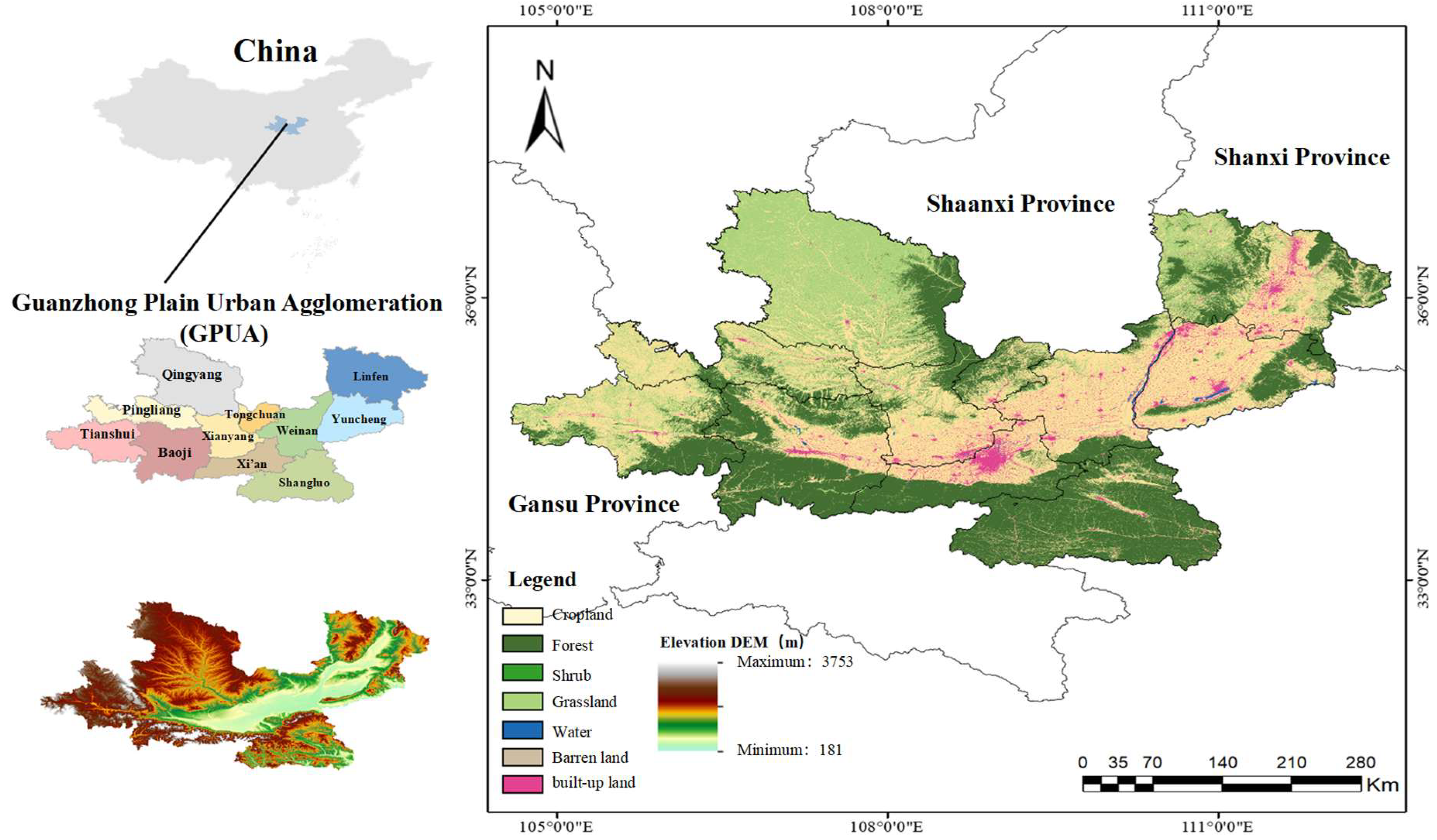
The Guanzhong Plain Urban Agglomeration (GPUA) is located in Northwest China (106°20′–111°15′ E, 33°35′–36°50′ N), situated in the middle reaches of the Yellow River Basin and serving as a crucial geographic hub connecting eastern and western China. The study area covers 107,100 km2, encompassing 11 prefecture-level cities across three provinces: six cities in Shaanxi Province (Xi’an, Baoji, Xianyang, Tongchuan, Weinan, and Shangluo), two cities in Shanxi Province (Yuncheng and Linfen), and three cities in Gansu Province (Tianshui, Pingliang, and Qingyang), as shown in Figure 2.
The region exhibits complex topographic diversity, including the Guanzhong Plain, Loess Plateau, Qinling Mountains, and Liupan Mountains, with elevations ranging from 345 m in the Wei River valley to 3767 m at Mount Taibai. The spatial distribution of land use reflects this topographic heterogeneity, with agricultural lands concentrated in the plains, forests dominating mountainous areas, and grasslands prevalent on the Loess Plateau. The study area is characterized by a temperate continental monsoon climate with distinct transitional features. Mean annual temperature ranges from 12 to 14 °C, with annual precipitation varying between 500 and 700 mm, showing significant spatial heterogeneity influenced by topography. From a socioeconomic perspective, the GPUA represents a vital economic growth pole in Western China, supporting approximately 40 million residents and generating a GDP exceeding 2.25 trillion yuan as of 2020. Xi’an, as the core city, has experienced rapid urban expansion, with its built-up area expanding from 186 km2 in 2001 to 683 km2 in 2021, exemplifying the intense urbanization pressure faced by the region.

3.1.2. Data Collection and Preprocessing

This study integrates multi-source heterogeneous data spanning 2001–2021 to construct a comprehensive database for analyzing PLE space evolution, as shown in Table 1. All spatial data were standardized to 500 m resolution to ensure consistency across different sources.
Data preprocessing involved the following steps: (1) Coordinate system standardization: all spatial data were projected to Albers Equal Area Conic projection (central meridian 105° E, standard parallels 25° N and 47° N) to ensure accurate area calculations; (2) Spatial resolution harmonization: all raster data were resampled to 500 m resolution using nearest neighbor or bilinear interpolation methods; (3) Data normalization: continuous variables were standardized using Z-score transformation to eliminate dimensional effects; (4) Missing value imputation: spatial or temporal interpolation methods were applied to fill data gaps; (5) Outlier detection: local spatial autocorrelation analysis was used to identify and correct anomalous values.
The land use classification data derived from the China Land Cover Dataset (CLCD) achieved an overall accuracy of 79% in the original validation. While this accuracy is below the ideal threshold of 90%, it represents one of the highest levels among available national-scale land use products and is sufficient for regional-scale analysis. However, this accuracy limitation may introduce uncertainties, particularly in complex landscape types such as peri-urban transitional zones where mixed pixels are common. To minimize error propagation, we implemented additional quality control measures including visual interpretation validation of randomly sampled locations (n = 500) and temporal consistency checks across multiple years to identify and correct systematic misclassifications.
The decision to harmonize all data to 500 m resolution was based on three considerations. First, while the original CLCD data at 30 m resolution provides fine spatial detail, processing such high-resolution data across the entire study area (158,000 km2) and 20-year time series would be computationally prohibitive without commensurate analytical benefits at the urban agglomeration scale. Second, most driving factor datasets (e.g., climate, socioeconomic data) have native resolutions of 1000 m; resampling to 500 m represents a compromise that avoids both excessive upscaling of land use data and the creation of pseudo-precision through aggressive downscaling of coarser covariates. Third, 500 m resolution effectively captures macro-scale pattern changes at the urban agglomeration level, which is the primary analytical focus. We acknowledge that this choice involves trade-offs: some spatial details in peri-urban fringes may be lost, but the selected resolution balances analytical needs with data processing efficiency and inter-dataset compatibility.
All spatial data processing and analysis were performed in an integrated technical environment to ensure computational efficiency and methodological consistency. Spatial data preprocessing, including coordinate system transformation, resolution resampling, and raster calculations, was conducted using QGIS 3.38.2 (QGIS Development Team, 2024). Random Forest analysis and statistical computations were implemented in Python 3.8.10 environment with scikit-learn (v0.24.2) and numpy (v1.20.3) libraries. The PLUS model simulations employed PLUS V1.0 software. All computations were executed on a workstation equipped with an Intel Core i7-7700 processor (3.60 GHz base frequency) and 64 GB RAM, providing sufficient computational capacity for processing high-resolution raster data across the 158,000 km2 study area over the 20-year analysis period. The complete model calibration and validation workflow (2001–2021) required approximately 18 h of computational time, while individual scenario projections (2021–2031) were completed within 3–4 h.

3.2. Analytical Framework

3.2.1. Production-Living-Ecological Space Classification System

Based on the principle of dominant land use functions and following the National Standard for Current Land Use Classification (GB/T 21010-2017) [77] and existing research, we developed a PLE space classification and evaluation system. The classification adheres to four principles: (1) Dominant functionality: spatial types are determined by primary land use functions; (2) Completeness: all land use types are assigned to appropriate spatial categories; (3) Mutual exclusivity: each land unit belongs to only one spatial type; (4) Operability: classification criteria are explicit and practically applicable.
The study employed a combination of expert scoring and analytic hierarchy process to quantitatively evaluate the production, living, and ecological functions of each land use type. A five-level scoring system was adopted: 0 points indicate absent function, 1 point indicates weak function, 3 points indicate moderate function, and 5 points indicate prominent function, as shown in Table 2. By calculating scores for each land use type across the three functions, spatial types were determined based on the highest score principle. The classification results are as follows: Production space includes paddy fields, dry farmland, and partial water bodies (rivers and reservoirs); Living space comprises urban land, rural settlements, and other construction land; Ecological space encompasses forest land, shrubland, sparse woodland, other woodland, grassland with varying coverage, beaches, wetlands, and barren land.
To validate the classification system’s rationality, we applied spatial autocorrelation analysis to examine the clustering degree of similar spaces. The global Moran’s I index is calculated as:
I = n i = 1 n     j = 1 n     w i j ( x i x ) ( x j x ) i = 1 n     j = 1 n     w i j i = 1 n     ( x i x ) 2
where n is the number of spatial units, x i and x j are attribute values of spatial units i and j , x is the mean attribute value, and w i j represents elements of the spatial weight matrix. The spatial weight matrix was constructed using Queen contiguity rules considering first-order neighbors, following standard practices in land use spatial analysis [78]. Results show that Moran’s I indices for all three space types exceed 0.6 (p < 0.01), indicating significant spatial clustering and validating the classification system.

3.2.2. Spatial Pattern Evolution Analysis

(1)
Spatial Gravity Center Migration Model
The spatial gravity center is a crucial indicator for describing the spatial distribution of geographic features, with its migration trajectory directly reflecting the evolution direction of spatial patterns. We calculated the gravity center coordinates of PLE spaces for each period using the weighted average method:
X t = i = 1 n     A i t X i i = 1 n     A i t
Y t = i = 1 n     A i t Y i i = 1 n     A i t
where ( X t , Y t ) represents the gravity center coordinates of a specific space type in year t , A i t is the area of patch i in year t , ( X i , Y i ) denotes the geometric center coordinates of patch i , and n is the total number of patches. The migration distance is calculated using Euclidean distance:
D t 1 , t 2 = ( X t 2 X t 1 ) 2 + ( Y t 2 Y t 1 ) 2
This weighted centroid approach has been widely applied in analyzing spatial shifts in urban expansion, population distribution, and economic activities [79,80]. Where D t 1 , t 2 represents the gravity center migration distance from period t 1 to period t 2 .
(2)
Land Use Transfer Matrix
The land use transfer matrix quantitatively describes the mutual conversion relationships among different land types across periods, serving as a classical method for analyzing land use changes. The mathematical expression of the transfer matrix is:
S i j = S 11 S 12 S 1 n S 21 S 22 S 2 n S n 1 S n 2 S n n
where S i j represents the area converted from land type i at the beginning to land type j at the end of the study period, and n is the number of land use types. Diagonal elements indicate unchanged areas, while off-diagonal elements represent converted areas.
Based on the transfer matrix, we further calculated land use dynamic indices. The single land use dynamic degree reflects the change rate of a specific land type:
K = U b U a U a × 1 T × 100 %
where K is the land use dynamic degree, U a and U b represent the area of a specific land type at the beginning and end of the study period, and T is the time span in years. The comprehensive land use dynamic degree reflects the overall rate of regional land use change:
L C = i = 1 n     Δ L U i j 2 i = 1 n     L U i × 1 T × 100 %
The transfer matrix approach follows the framework, while the dynamic degree indicators are adapted and have been extensively applied in China’s land use change studies [81,82]. Where L C is the comprehensive land use dynamic degree, L U i is the area of land type i at the beginning, and Δ L U i j is the absolute value of area converted from type i to other types during the study period.
(3)
Land Use Intensity Spectrum Analysis
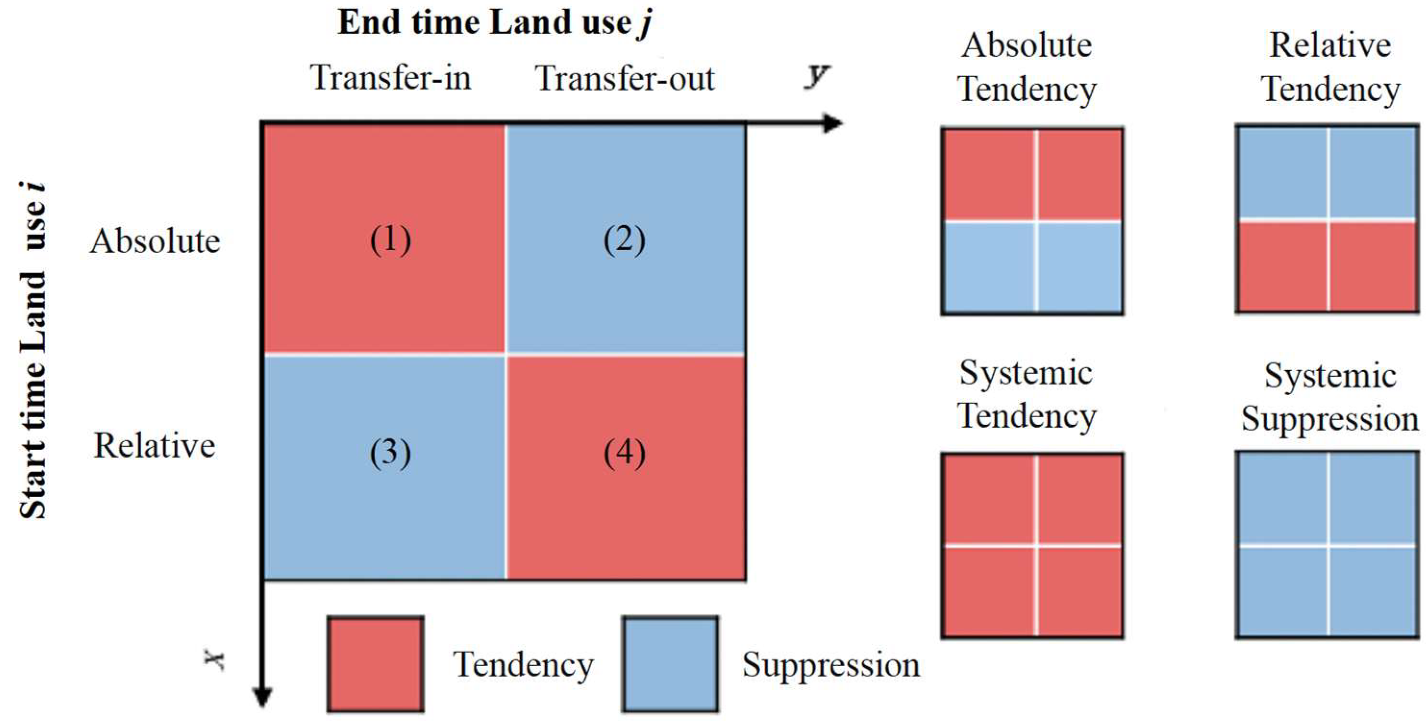
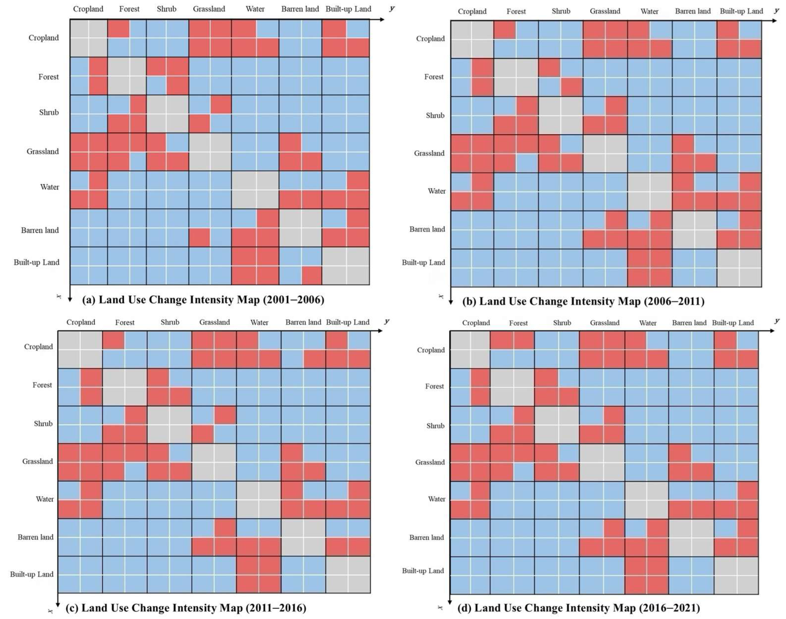
To reveal the systematic characteristics of land use transitions, the study constructed a land use intensity spectrum analysis framework. This framework encompasses two dimensions (absolute and relative intensity) and two directions (gain and loss), forming a four-element analysis matrix, as shown in Figure 3.
Absolute gain intensity is defined as:
R i j = S i j T J
where R i j is the absolute intensity of transition from land type i to type j , T is the time interval, and J is the total study area. Relative gain intensity is defined as:
W i j = S i j k j     S k j
where W i j is the relative intensity of transition from land type i to type j .
By comparing actual transition intensity with average transition intensity, the study identifies systematic tendencies or constraints in transition processes. When all four intensity indicators show tendency, the study defines it as systematic tendency; otherwise, it represents systematic constraint.

3.2.3. Driving Factor Identification

The study employed Random Forest (RF) algorithm to identify driving factors of PLE space evolution. Random Forest is an ensemble learning method that constructs multiple decision trees and aggregates their predictions, effectively handling high-dimensional data, nonlinear relationships, and variable interactions.
The core principle involves generating multiple training subsets through Bootstrap sampling, with each subset used to train a decision tree. During node splitting, a subset of features is randomly selected, and the optimal feature is chosen for splitting. Final predictions are obtained through voting (classification) or averaging (regression) across all trees.
Variable importance is assessed by calculating Out-of-Bag (OOB) error:
V I j = 1 N i = 1 N   ( e i j p e r m e i j )
where V I j is the importance of variable j , N is the number of decision trees, e i j is the original OOB error of tree i , and e i j p e r m is the OOB error after permuting variable j .
Model parameters were set following best practices and subsequent land use modeling studies [83]: 500 decision trees (determined through convergence testing where OOB error stabilized beyond 300 trees), maximum depth of 20 layers (balancing overfitting risk against predictive accuracy), minimum leaf node samples of 5, and feature sampling ratio equal to √ P where P is the total number of features (17 in this study). We applied 10-fold cross-validation to optimize parameters and ensure model generalization capability [84]. The choice of 500 trees balances predictive accuracy and computational efficiency [85].

3.3. Markov Chain-PLUS Coupled Model and Scenario Design

3.3.1. Markov Chain Model

The Markov chain model predicts quantitative changes in land use based on state transition probabilities. The model assumes that land use state transitions depend only on current states, independent of historical paths (Markov property). The state transition probability matrix is calculated as:
P i j = N i j j = 1 m     N i j
where P i j is the probability of transition from state i to state j , N i j is the number of pixels transitioning from state i to state j during the observation period, and m is the total number of states. Future land use states are predicted using:
S ( t + 1 ) = S ( t ) × P
where S ( t ) and S ( t + 1 ) are state vectors at time t and t + 1 , and P is the state transition probability matrix. To improve prediction accuracy, we employed weighted averaging of multi-period transition probability matrices:
P a v g = k = 1 n 1   w k P k
The Markov chain model has been extensively applied in land use change projection due to its ability to capture transition probabilities while maintaining computational simplicity [86].
We employed a time-weighted averaging approach to account for accelerating urbanization trends in recent periods, assigning higher weights to more recent transition matrices (2016–2021: weight = 0.4; 2011–2016: weight = 0.3; 2006–2011: weight = 0.2; 2001–2006: weight = 0.1). Where P a v g is the average transition probability matrix, P k is the transition probability matrix for period k , and w k represents weight coefficients determined using inverse time weighting.

3.3.2. PLUS Model Principles and Implementation

The PLUS model comprises two core modules: Land Expansion Analysis Strategy (LEAS) and CA based on Multi-type Random Seeds (CARS). The LEAS module analyzes expansion patterns of each land type through random forest algorithms, calculating development probability:
P i , k d = n = 1 M   I { h n ( x ) = d } M
where P i , k d is the development probability of pixel i converting to land type d at iteration k , M is the total number of decision trees, h n ( x ) is the prediction of tree n , and I { } is the indicator function.
The CARS module employs roulette wheel selection and threshold-decreasing rules to simulate spatial land use allocation:
T P i , k d = P i , k d × Ω i , k d × D k d
where T P i , k d is the combined probability, Ω i , k d is the neighborhood effect, and D k d is the conversion difficulty coefficient.
Neighborhood effects are calculated using Moore neighborhoods:
Ω i , k d = N × N     c o n ( c i t 1 = d ) N × N 1 × w d
where c o n ( ) is the counting function, c i t 1 is the land type of pixel i at time t 1 , N is the neighborhood window size, and w d is the neighborhood weight for land type d .
The threshold-decreasing rule controls new patch generation:
τ k = τ 0 × ( 1 k K ) δ
where τ k is the threshold at iteration k , τ 0 is the initial threshold, K is the total number of iterations, and δ is the decreasing rate parameter.

3.3.3. Multi-Scenario Parameter Settings

Based on regional development characteristics and policy orientations, we designed four development scenarios:
(1)
Natural Evolution Scenario (NES): Maintains historical land use transition trends without additional policy interventions. Transition probabilities use 2001–2021 averages, with default neighborhood weights and conversion costs.
(2)
Urban Development Priority Scenario (UDPS): Emphasizes economic construction and urban expansion. Increases conversion probability from cropland and grassland to built-up land by 30%, reduces built-up land conversion cost by 20%, and sets built-up land neighborhood weight to 1.2.
(3)
Food Security Priority Scenario (FSPS): Strictly protects basic farmland to ensure food production capacity. Reduces conversion probability from cropland to other land uses by 60%, establishes basic farmland protection zones as conversion-restricted areas, and sets cropland neighborhood weight to 1.1.
(4)
Ecological Protection Priority Scenario (EPPS): Strengthens ecological space protection and restoration. Reduces conversion probability from forest and grassland to other land uses by 50%, sets ecological land neighborhood weight to 1.3, and establishes conversion restrictions in ecological redline areas.
Model validation used 2001–2016 data for training and predicted 2021 land use patterns for comparison with actual data. Accuracy assessment metrics include:
Overall Accuracy:
O A = i = 1 n     x i i i = 1 n     j = 1 n     x i j
Kappa coefficient:
K a p p a = P o P e 1 P e
where P o is observed agreement and P e is expected agreement.
Figure of Merit (FoM):
F O M = B A + B + C + D
where B represents the area of correctly predicted change (intersection of simulated and actual changes), A is the area of false alarm (simulated change but no actual change), C is the area of misses (actual change but not simulated), and D is the area of wrong hits (change predicted and occurred but to different land use types). F O M values range from 0 to 1, with higher values indicating better simulation accuracy for spatial change locations.
Through the integrated application of this methodological framework, this study establishes a complete technical workflow from data preparation, spatial analysis, and driver identification to scenario simulation, providing scientific support for understanding PLE space evolution mechanisms and formulating differentiated spatial optimization strategies in the Guanzhong Plain Urban Agglomeration.

4. Results

4.1. Spatiotemporal Evolution of PLE Space Patterns

4.1.1. Spatial Distribution and Structural Changes

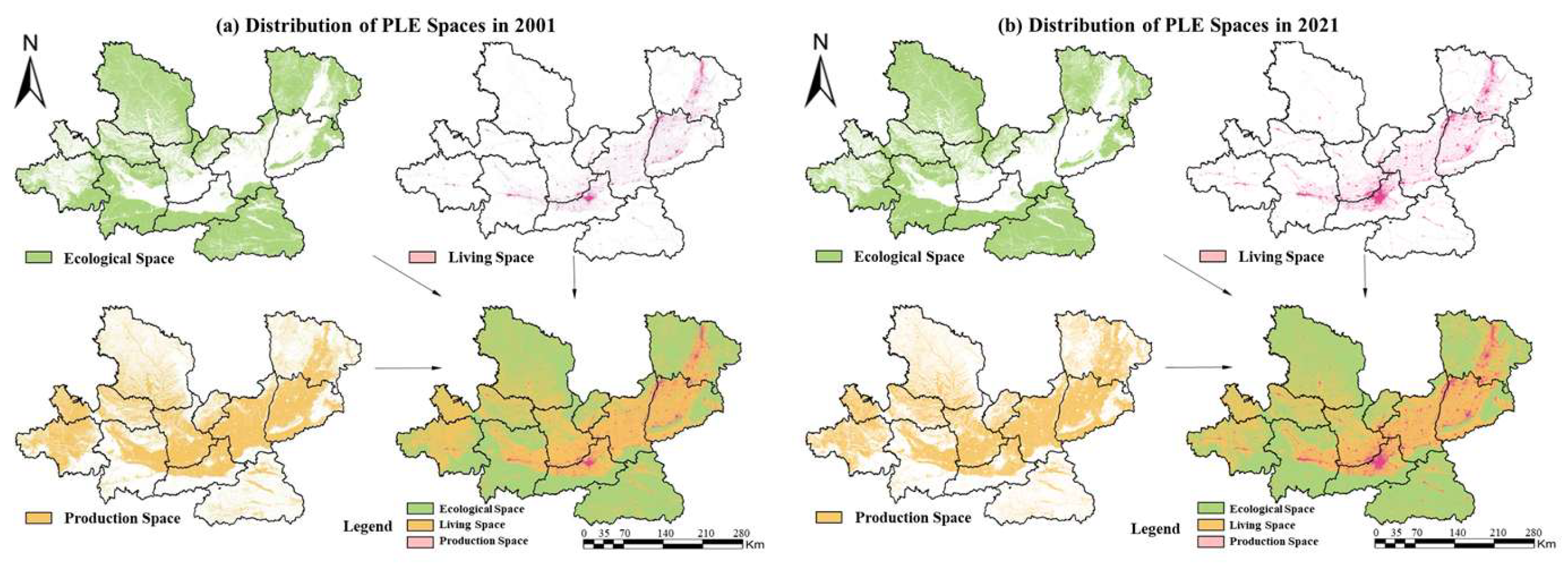
The PLE space distribution in the GPUA exhibited significant spatiotemporal heterogeneity from 2001 to 2021, as shown in Figure 4.
Production space decreased from 68,700 km2 in 2001 to 63,570 km2 in 2021, representing a 7.47% decline. Living space expanded dramatically from 4060 km2 to 7060 km2, achieving a 73.89% increase. Ecological space contracted from 34,340 km2 to 31,270 km2, a reduction of 8.94%. These changes reflect the intense competition for land resources driven by rapid urbanization and economic development. Maps show the evolution of production space (yellow), living space (red), and ecological space (green) at five-year intervals, revealing the expansion of urban areas and the transformation of agricultural and ecological lands.
The spatial configuration of PLE spaces in 2021 reveals distinct geographic patterns, as shown in Table 3. Production space is predominantly concentrated in the Wei River Plain and Fen River Valley, with Yuncheng (9275 km2, 14.59%), Weinan (9063 km2, 14.26%), and Linfen (7661 km2, 12.05%) accounting for the largest shares. Living space shows strong concentration in core cities, with Xi’an (1358 km2, 19.24%), Yuncheng (1502 km2, 21.29%), and Weinan (1165 km2, 16.51%) dominating the distribution. Ecological space is primarily located in mountainous and plateau regions, with Qingyang (21,135 km2, 23.14%), Shangluo (17,316 km2, 18.96%), and Baoji (12,219 km2, 13.38%) containing the largest areas.
The urban expansion patterns revealed significant spatial agglomeration, particularly around Xi’an and its satellite cities, as shown in Figure 5.
The Xi’an metropolitan area experienced big transformation, with its built-up area expanding from 186 km2 in 2001 to 683 km2 in 2021, representing a 267% increase. This expansion followed major transportation corridors, creating ribbon-like development patterns along highways and railways. The maps illustrate the progressive expansion of Xi’an’s urban footprint and the gradual integration with surrounding cities including Xianyang, forming an increasingly connected metropolitan region.

4.1.2. Gravity Center Migration Trajectories

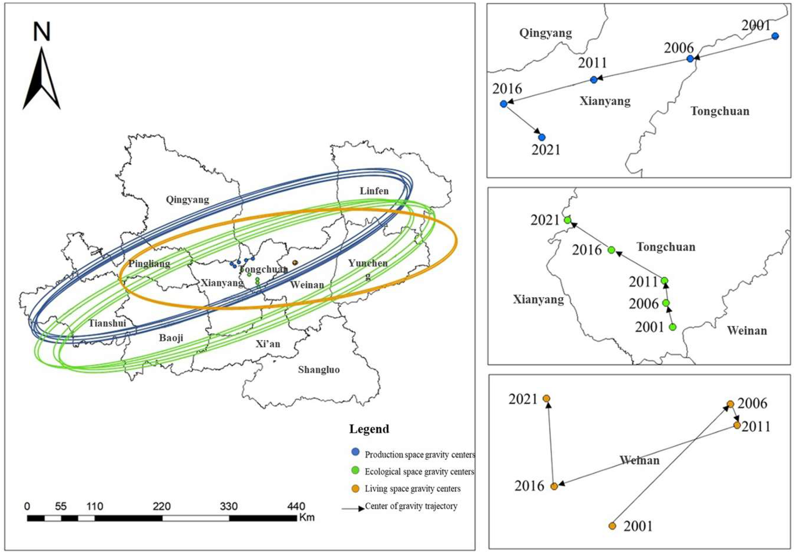
The gravity centers of PLE spaces exhibited distinct migration patterns over the study period, reflecting the asymmetric nature of regional development, as shown in Figure 6.
Production space gravity center migrated 23.4 km southwest, driven by agricultural intensification in western counties and the conversion of eastern farmlands to urban uses. Living space gravity center remained relatively stable, shifting only 1.2 km northeast, indicating the persistence of established urban hierarchies. Ecological space gravity center moved 18.9 km northwest, influenced by ecological restoration projects in the northern Loess Plateau and forest conservation in the Qinling Mountains. Arrows indicate the direction and magnitude of shifts, with production space showing southwestern migration, ecological space moving northwest, and living space remaining relatively stable.

4.2. Land Use Transfer Dynamics and Intensity Analysis

4.2.1. Land Use Transfer Patterns

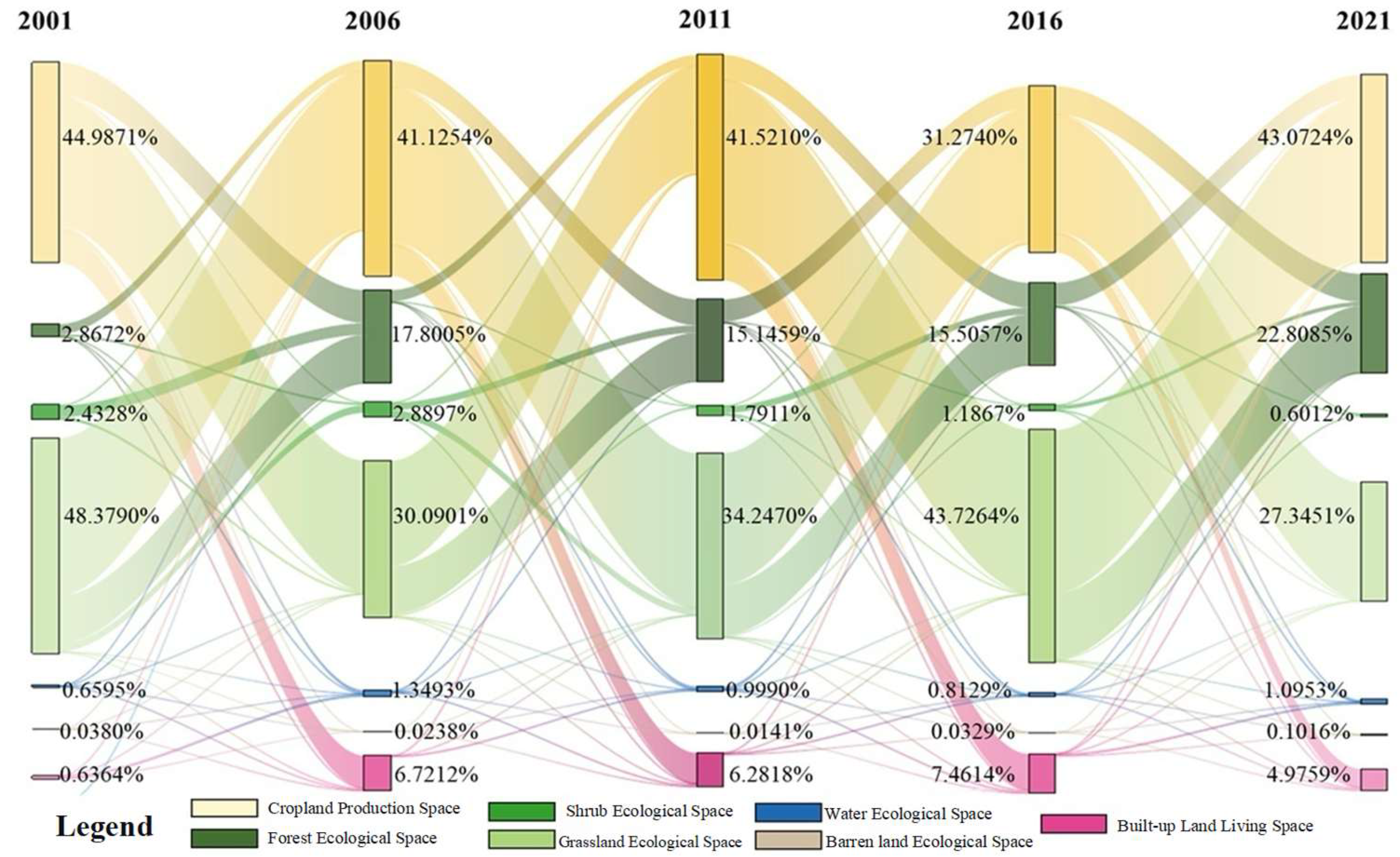
The land use transfer analysis revealed complex conversion patterns across four transition periods, as shown in Figure 7. The width of flows represents the magnitude of transfers, highlighting the dominant transitions from cropland and grassland to built-up land, and the complex exchanges between agricultural and ecological lands.
Total transferred area reached 46,500 km2 over 2001–2021, with the highest transfer intensity occurring during 2011–2016 (26.56% of total transfers). Cropland experienced the largest outflow (19,900 km2), primarily converting to built-up land (42.3%) and grassland (31.2%). Grassland showed net losses of 19,500 km2, mainly transitioning to cropland (48.7%) and forest (26.4%). Built-up land achieved net gains of 3000 km2, with 68.5% sourced from cropland and 19.3% from grassland.

4.2.2. Land Use Dynamic Degrees

The analysis of land use dynamic degrees revealed varying rates of change across different land types and periods, as shown in Table 4.
Built-up land exhibited the highest single dynamic degree throughout all periods, peaking at 3.93% annually during 2001–2006. Water bodies showed significant volatility, with dynamic degrees ranging from −0.93% to 5.39%. Forest areas demonstrated consistent growth (0.54–0.79% annually), while shrubland experienced severe contraction (−15.32% over the entire period).
The comprehensive land use dynamic degree remained relatively stable (0.14–0.19%), indicating consistent overall change intensity despite variations in individual land types. The slight increase in 2016–2021 (0.18%) suggests accelerating land use transitions in recent years, potentially driven by intensified urbanization and ecological restoration policies.

4.2.3. Land Use Intensity Spectrum Evolution

The intensity spectrum analysis revealed systematic patterns in land use transitions across different periods, as shown in Figure 8. During 2001–2006, cropland-to-built-up and grassland-to-cropland transitions showed systematic tendency (all four intensity indicators positive), indicating strong driving forces. Forest-to-shrub land and shrub land-to-grass land transitions exhibited absolute tendency but relative constraint, suggesting localized but not widespread changes.
Red cells indicate systematic tendency, blue cells show systematic constraint, and mixed colors represent partial tendency or constraint. The intensity of colors reflects the magnitude of transition strengths. The 2006–2011 period witnessed reduced ecological pressure, with forest to shrub land transitions losing their absolute tendency. However, urban expansion maintained strong momentum, with cropland-to-built-up transitions retaining systematic tendency. The 2011–2016 period showed intensified land use unsustainability, with multiple ecological transitions exhibiting systematic constraints.
Notably, 2016–2021 marked a turning point, with grassland-to-forest transitions achieving absolute tendency, reflecting successful ecological restoration initiatives. This period coincided with the implementation of the Guanzhong Plain Urban Agglomeration Development Plan (2018), which established ecological redlines and strengthened environmental protection measures.

4.3. Driving Mechanisms of PLE Space Evolution

4.3.1. Driving Factors of Cropland Production Space Expansion

The expansion of cropland production space demonstrates a complex multifactorial relationship, with annual precipitation, population density, GDP, distance to secondary urban roads, annual mean temperature, and elevation DEM emerging as the most influential determinants, as shown in Figure 9. Annual precipitation exhibits the highest contribution coefficient (0.132), followed by population density (0.108), indicating that hydrological availability and demographic pressure constitute the primary drivers of agricultural land expansion. This empirical finding corroborates the spatial distribution pattern whereby newly established cropland production spaces predominantly manifest in areas characterized by relatively low elevation and substantial distance from urban commercial centers. This phenomenon is particularly pronounced in the peripheral zones of major municipalities, including Xi’an, Xianyang, and Weinan.
Secondary driving factors encompass GDP (0.107), distance to secondary urban infrastructure (0.094), annual mean temperature (0.087), and elevation DEM (0.083), collectively demonstrating the intricate interdependence between agricultural spatial patterns and climatic, topographic, and anthropogenic variables within the Guanzhong Plain Urban Agglomeration. The spatial distribution of cropland exhibits preferential concentration in regions characterized by adequate precipitation regimes, sufficient labor force availability, and optimal distance from secondary urban transportation networks.
The progressive temperature increment observed within the study area induces elevated atmospheric water demand and intensifies evapotranspiration processes, simultaneously affecting vegetation phenology and reconfiguring cropland production space expansion trajectories. The positive correlation between local GDP growth and cropland expansion reflects the synergistic effects of development-induced land demand and agricultural technological advancement. Furthermore, proximity to secondary urban roads significantly influences agricultural land distribution patterns, as these corridors typically concentrate anthropogenic activities, rendering cropland production space evolution most pronounced in zones experiencing intensive human perturbation.

4.3.2. Driving Factors of Forest Ecological Space Expansion

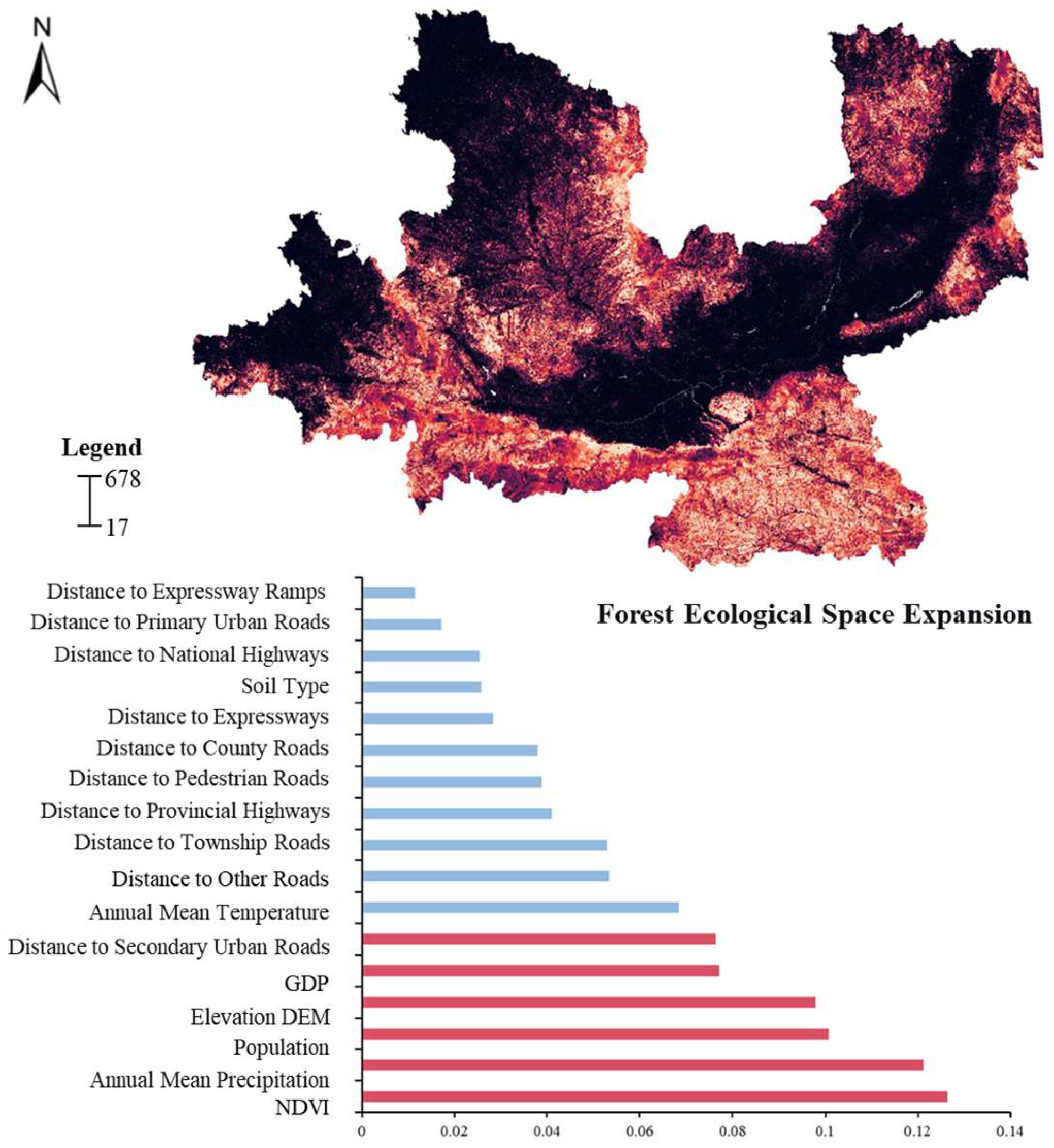
Forest ecological space expansion within the Guanzhong Plain Urban Agglomeration exhibits multifactorial determination, as shown in Figure 10. The Normalized Difference Vegetation Index (NDVI), serving as a proxy for ecosystem vitality, demonstrates the highest contribution coefficient (0.126), succeeded by annual precipitation (0.121). These primary determinants underscore the fundamental role of climatic and ecological conditions in mediating forest spatial expansion dynamics. Population density and elevation DEM contribute significantly (0.106 and 0.098, respectively), indicating that forest ecological spaces preferentially establish in topographically complex areas with reduced anthropogenic pressure.
Economic activity, as measured by GDP, exerts moderate influence on forest expansion (0.077), suggesting that regions experiencing economic prosperity demonstrate enhanced capacity for forest conservation and sustainable management initiatives. The contribution of distance to secondary urban roads (0.076) reveals a positive spatial correlation, attributable to diminished anthropogenic disturbance in remote locations.
Forest ecological space expansion exhibits distinct spatial heterogeneity compared to cropland distribution, concentrating primarily in ecologically vulnerable high-altitude regions including the Qinling Mountains and Lüliang Mountains, as well as the Loess Plateau, which has experienced historical ecological degradation due to intensive human activities. These regions are characterized by sparse forest resources, heterogeneous coverage patterns, and pronounced altitudinal gradients. This distribution pattern reflects deliberate policy intervention and ecological restoration initiatives rather than stochastic processes. Within the spatial architecture of the Guanzhong Plain Urban Agglomeration, newly expanded grassland, shrubland, and aquatic ecological spaces frequently adjoin or encompass forest ecological zones. This spatial configuration can be attributed to forest ecosystems’ function as hydrological regulation zones, indirectly facilitating the systematic development of complementary ecosystems through watershed management processes.

4.3.3. Driving Factors of Shrubland Ecological Space Expansion

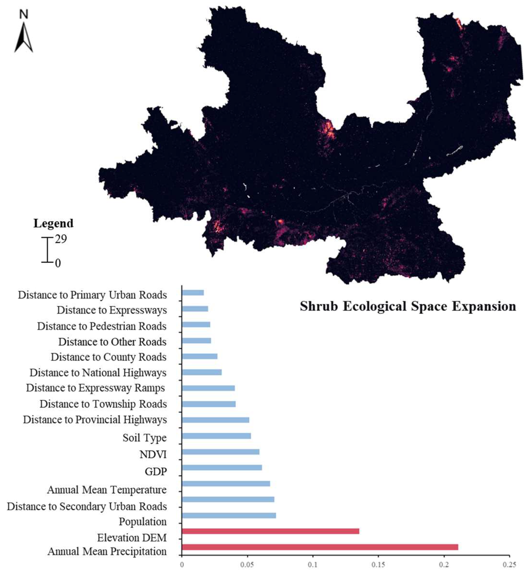
Figure 11 shows the multifactorial influences governing shrubland ecological space expansion within the Guanzhong Plain Urban Agglomeration. Annual precipitation emerges as the predominant determinant (0.211), establishing a direct causal relationship between hydrological availability and shrubland establishment. Precipitation functions not only as a prerequisite for shrubland development but also determines the velocity and spatial extent of ecological expansion through temporal and spatial distribution patterns.
Elevation DEM contributes substantially (0.135), emphasizing topographic constraints as a critical determinant. Shrubland communities established at higher altitudes typically demonstrate enhanced growth potential and expansion rates, particularly within specific geomorphological contexts such as the Loess Plateau and Qinling Mountains. These fundamental driving mechanisms provide explanatory frameworks for shrubland ecological space expansion phenomena while establishing scientific foundations for territorial spatial planning and ecological conservation strategies. Considering the influence of precipitation and topographic variables, priority should be accorded to shrubland vegetation protection and restoration in high-precipitation, high-elevation zones. Simultaneously, these areas warrant inclusion in ecologically vulnerable zone classifications to secure enhanced governmental support and financial investment.

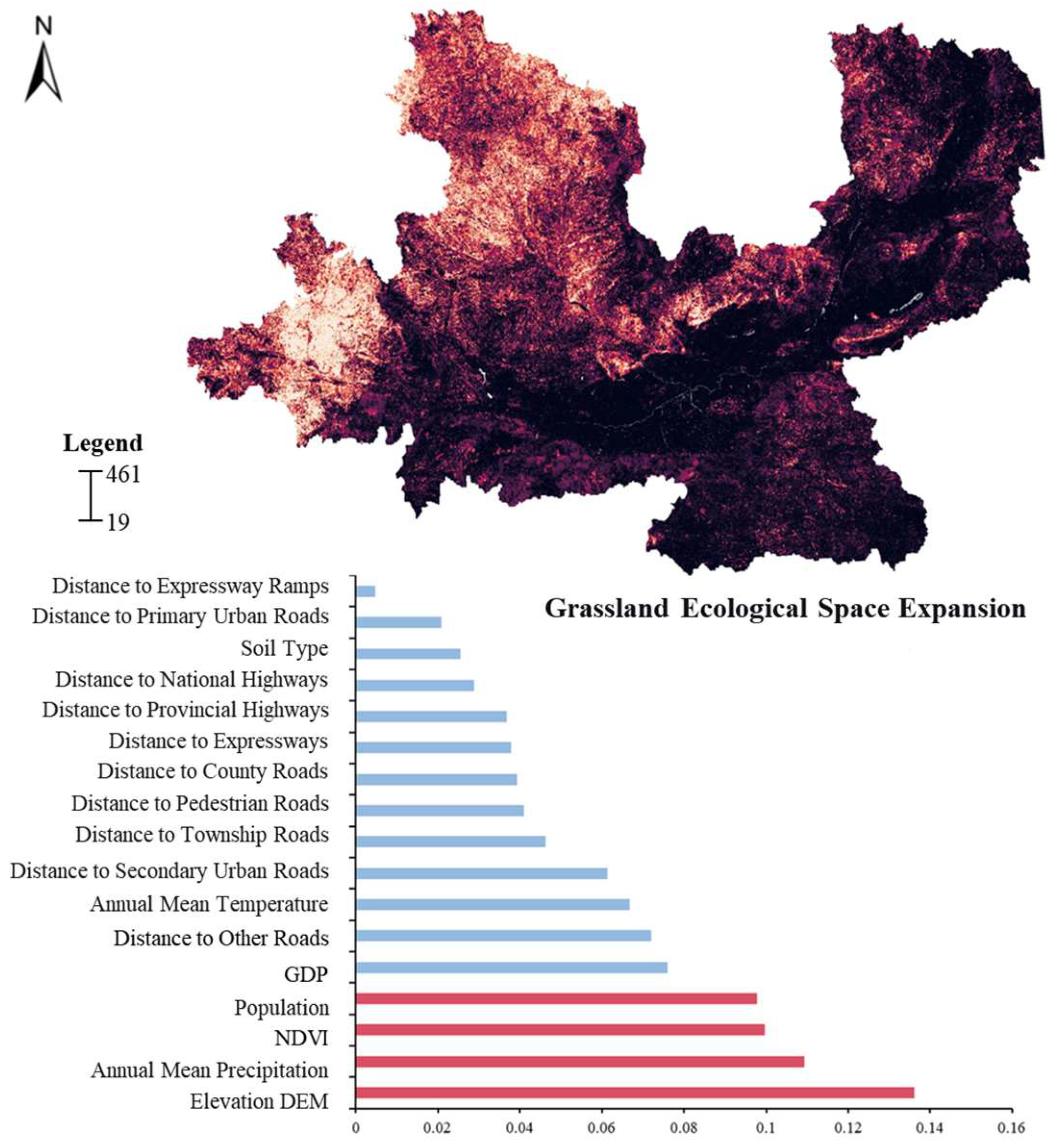
4.3.4. Driving Factors of Grassland Ecological Space Expansion

Investigation of grassland ecological space expansion within the Guanzhong Plain Urban Agglomeration, as shown in Figure 12, reveals elevation DEM and annual precipitation as the most influential determinants, with contribution coefficients of 0.136 and 0.109, respectively. These findings underscore the paramount importance of climatic and topographic variables in grassland distribution while highlighting the distinctive contribution of high-altitude regions to grassland ecosystem establishment. The significant influence of elevation DEM indicates that grassland ecosystems demonstrate preferential distribution at higher altitudes, correlating with reduced anthropogenic activities and diminished land use intensity in montane environments. The substantial contribution of annual precipitation confirms that hydrological supply constitutes a critical prerequisite for grassland ecosystem maintenance and expansion.
Secondary factors, including distances to various road classifications, exhibit relatively diminished contribution coefficients, indicating that grassland ecological spaces typically establish in locations remote from anthropogenic activity centers. This observation provides valuable insights for territorial spatial planning and ecological conservation initiatives. Grassland ecological space expansion phenomena are particularly pronounced in the Longdong Plateau, Loess Plateau, and Liupan Mountains. Within the Loess Plateau region, characterized by elevations ranging from 1000 to 2000 m, grassland coverage encompasses approximately 350 million mu, representing one-third of the regional land area and contributing 7.4% of China’s total grassland resources. However, this region currently confronts severe challenges including grassland degradation and ecological deterioration, resulting in substantial area reduction and compromised ecological quality.
The comprehensive analysis provides profound insights into grassland ecological space expansion determinants while emphasizing the decisive roles of altitude and precipitation. This establishes robust scientific foundations for subsequent territorial spatial planning and ecological restoration initiatives, particularly when addressing the increasingly severe degradation of grassland ecosystems.

4.3.5. Driving Factors of Water Ecological Space Expansion

Analysis of water ecological space expansion within the Guanzhong Plain Urban Agglomeration, as shown in Figure 13, identifies elevation DEM and annual mean temperature as the most significant determinants. Elevation DEM exhibits the highest contribution coefficient (0.229), followed by annual mean temperature (0.188).
The pronounced influence of elevation DEM indicates that water ecological space expansion predominantly occurs in low-lying terrain or areas with gentle topographic gradients, as well as high-altitude valley systems. This phenomenon correlates directly with geomorphological and climatic conditions while reflecting regional hydrological cycles and groundwater dynamics. Annual mean temperature exerts substantial influence; elevated temperatures increase evaporation rates while simultaneously affecting hydrological cycles and precipitation patterns, ultimately inducing modifications in aquatic surface areas.
Beyond natural determinants, demographic factors moderately influence water ecological space expansion. This relationship demonstrates high concordance with the socioeconomic characteristics of the study region, particularly evident in areas surrounding the Wei River, where aquatic expansion phenomena are most pronounced. The Wei River, functioning as the ecological and economic lifeline of the Guanzhong Plain, connects major municipalities including Baoji, Xi’an, Xianyang, Weinan, Yuncheng, and Linfen. Water ecological space evolution affects not only local ecosystem integrity but also exerts substantial impacts on the economic and social development trajectories of these urban centers.

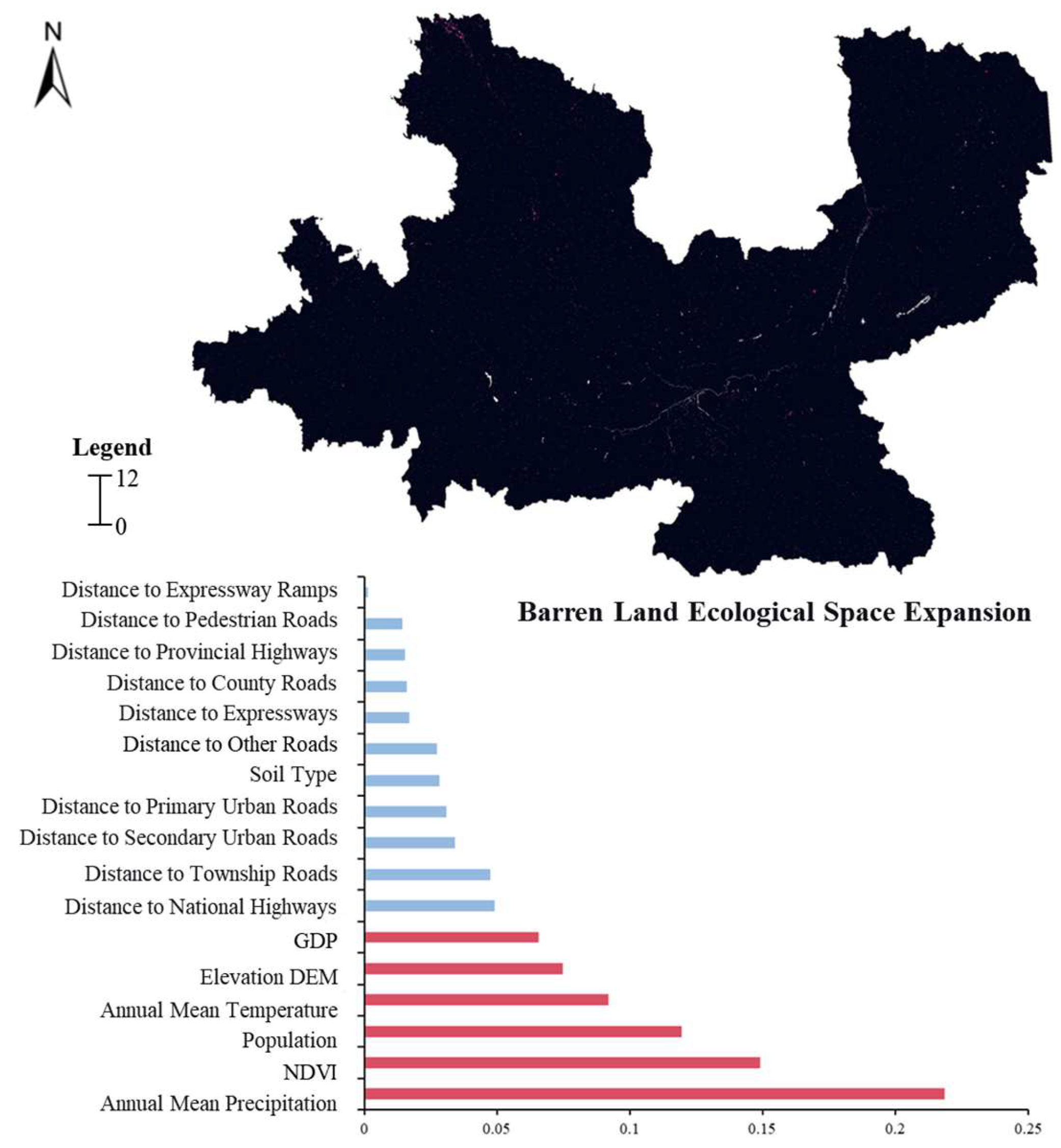
4.3.6. Driving Factors of Barren Land Ecological Space Expansion

Comprehensive investigation of barren land ecological space distribution within the Guanzhong Plain Urban Agglomeration includes quantitative assessment of individual driving factor contributions, as shown in Figure 14. Annual precipitation emerges as the paramount determinant (0.228), establishing a critical observation: barren land demonstrates preferential distribution in precipitation-deficient regions, where hydrological scarcity induces soil impoverishment and inadequate vegetation coverage.
NDVI and population density constitute the secondary and tertiary influential factors, with contribution coefficients of 0.149 and 0.134, respectively, illustrating the complex interactions between ecological and anthropogenic variables. The substantial contribution of NDVI indicates that barren land ecological space expansion zones are characterized by extremely sparse vegetation coverage. Simultaneously, the significant influence of population density reflects anthropogenic activities, including inappropriate land utilization and development practices, which induce land degradation and transformation to barren conditions.
Annual mean temperature, elevation DEM, and GDP exert moderate influences on barren land ecological space expansion, with contribution coefficients of 0.092, 0.075, and 0.065, respectively. Annual mean temperature correlates with soil evaporation processes and vegetation establishment, while elevation and GDP relate to land utilization patterns and economic activities. During the 2001–2021 period, barren land demonstrated pronounced expansion trends in specific areas of the Guanzhong Plain Urban Agglomeration, most notably along the Wei River banks in Xi’an Municipality. This phenomenon reflects both natural environmental influences and correlations with local land use policies, excessive demographic concentration, and inappropriate development practices during this temporal period.

4.3.7. Driving Factors of Built-Up Living Space Expansion

Comprehensive quantitative analysis of factors influencing built-up living space expansion within the Guanzhong Plain Urban Agglomeration reveals several determinants exhibiting particularly significant influence, as shown in Figure 15. Population density emerges as the predominant factor (0.242), followed by elevation DEM (0.157). The significance of these variables emphasizes the fundamental influence of demographic agglomeration and topographic constraints on urban living space development trajectories.
Annual mean temperature demonstrates noteworthy correlation with built-up living space expansion (0.127), relating to regional climatic suitability for residential and industrial activities, particularly concerning winter heating and summer cooling requirements. GDP contributes moderately (0.093), indicating a definitive positive correlation between economic vitality and built-up living space expansion. This relationship suggests that regions experiencing rapid economic development typically demonstrate more urgent construction land demands. The relatively modest contribution of highway proximity to built-up land expansion indicates that within the spatial development strategy of the Guanzhong Plain Urban Agglomeration, transportation accessibility does not necessarily constitute a decisive determinant, or its influence may be overshadowed by more dominant factors.
Comprehensive consideration of multidimensional urban spatial expansion phenomena within the Guanzhong Plain Urban Agglomeration reveals that all spatial categories experience influence from multiple driving factors. These determinants encompass elevation DEM, annual precipitation, annual mean temperature, and population density. Annual precipitation and elevation DEM demonstrate significant influence across multiple spatial expansion categories, indicating that natural environmental factors maintain core roles in urban spatial evolution processes. Simultaneously, population density and GDP exhibit substantial socioeconomic influence in specific urban space expansions, particularly cropland production space and built-up living space. This comprehensive analysis provides holistic perspectives for understanding land utilization and urban spatial evolution within the Guanzhong Plain Urban Agglomeration while establishing scientific foundations for more precise and sustainable planning and management strategies targeting diverse land utilization categories.

4.4. Multi-Scenario Evolution Simulation Based on Markov Chain-PLUS Coupled Model

4.4.1. Model Validation and Accuracy Assessment

Prior to scenario simulation, rigorous validation of the Markov chain-PLUS coupled model was conducted using a split-sample approach. The model was trained using 2001–2016 land use data and employed to predict 2021 land use patterns, which were subsequently compared with observed data through multiple validation metrics.
Validation results demonstrated exceptional performance, as shown in Table 5. Overall Accuracy (OA) of 92.3%, Kappa coefficient of 0.91, and Figure of Merit (FoM) of 0.24. The Kappa coefficient of 0.91 indicates near-perfect agreement between predicted and observed land use patterns.
The FoM value of 0.24, while seemingly modest, is within the acceptable range for multi-class land use simulations. The FoM values typically range from 0.15 to 0.35 for complex landscape simulations, as this metric stringently evaluates only correctly predicted change pixels while penalizing false alarms and misses. Our FoM value indicates that approximately 24% of all predicted changes occurred in correct locations, comparable to values reported in similar studies using PLUS models.
Producer’s accuracy exceeded 85% for all land use categories, while user’s accuracy surpassed 83%, as shown in Table 6, confirming the model’s robust predictive capability and reliability for scenario projections. The high validation accuracy provides confidence in using the calibrated model for 2031 projections under different policy scenarios.
To assess the robustness of our modeling framework, we conducted sensitivity tests on key parameters for both the Random Forest and PLUS models.
For the Random Forest model, we tested three configurations of decision tree numbers (100, 300, 500) and three maximum feature settings (√p, p/3, p/2, where p = 17 driving factors). The rankings of the top five driving factors remained stable across all parameter combinations, with correlation coefficients >0.95 between importance scores. This stability confirms that our identification of dominant drivers (DEM, population density, distance to highways, GDP, NDVI) is not an artifact of parameter selection.
For the PLUS model, we evaluated the impact of neighborhood window size (1, 2, 3 pixels) and sampling strategy (random vs. stratified) on simulation accuracy. The Kappa coefficient ranged from 0.89 to 0.92 across these configurations, with our selected parameters (2-pixel neighborhood, stratified sampling) achieving optimal balance between computational efficiency and accuracy. FoM values showed similar stability (0.22–0.25), indicating that the model’s spatial prediction capability is robust to moderate parameter variations.
These sensitivity analyses provide confidence that our results are not highly dependent on arbitrary parameter choices and would be reproducible with reasonable alternative specifications. The high validation accuracy combined with parameter robustness provides strong foundation for using the calibrated model for 2031 projections under different policy scenarios.

4.4.2. Markov Chain Projection Results

Based on historical data spanning 2001–2021, the Markov chain model projected land use demand for each category within the Guanzhong Plain Urban Agglomeration through 2031, as shown in Table 7.
The projections reveal pronounced structural transformations in land use composition within the Guanzhong Plain Urban Agglomeration. Cropland demonstrates persistent contraction, declining from 63,574 km2 in 2021 to 56,204 km2 in 2031, representing an 11.59% reduction that reflects sustained urbanization pressure on agricultural lands. Built-up land exhibits rapid expansion, increasing from 7058 km2 in 2021 to 10,961 km2 in 2031, constituting a 55.34% growth that manifests robust regional economic development and demographic agglomeration.
Forest area displays an ascending trajectory, projected to reach 61,369 km2 by 2031, representing a 7.12% increase from 2021 levels. This expansion primarily attributes to sustained implementation of ecological civilization policies and afforestation programs. Water bodies initially increase before declining, contracting from 542 km2 in 2021 to 265 km2 in 2031, potentially correlating with climate variability and anthropogenic influences. Both grassland and shrubland demonstrate degenerative trends, decreasing by 11.92% and 17.64%, respectively, indicating ecological degradation pressures.
These projections provide the quantitative foundation for subsequent spatial allocation in the PLUS model under different policy scenarios, enabling exploration of alternative futures beyond the trend-continuation pathway.

4.4.3. Multi-Scenario Design and Parameter Configuration

Based on development characteristics and policy orientations within the GPUA, the study constructed four development scenarios to examine spatial evolution trajectories under different policy frameworks. Core characteristics and parameter configurations for each scenario are shown in Table 8.
(1)
Natural Evolution Scenario (NES)
This scenario extrapolates from historical evolution trends during 2001–2021 without introducing additional policy interventions, reflecting natural development trajectories of regional land use. Transition probabilities employ historical averages, with neighborhood weights and conversion costs utilizing default parameters, establishing a baseline for comparative analysis with other scenarios.
(2)
Urban Development Priority Scenario (UDPS)
This scenario emphasizes economic construction and urban expansion through moderate relaxation of built-up land expansion constraints. Transition probabilities from cropland and grassland to built-up land increase by 30% and 20%, respectively, built-up land conversion costs decrease by 20%, and built-up land neighborhood weight is set to 1.2 to promote compact urban development.
(3)
Food Security Priority Scenario (FSPS)
This scenario implements stringent basic farmland protection to ensure food production capacity. Transition probability from cropland to built-up land decreases by 60%, basic farmland protection zones are designated as conversion-restricted areas, cropland neighborhood weight is set to 1.1, while ecological restoration probability increases by 10%.
(4)
Ecological Protection Priority Scenario (EPPS)
This scenario strengthens ecological space protection and restoration while controlling unregulated built-up land expansion. Transition probabilities from forest and grassland to built-up land decrease by 50%, ecological land neighborhood weight is set to 1.3, conversion restrictions are established within ecological red line areas, and ecological restoration probability increases by 30%.

4.4.4. Scenario Simulation Results and Analysis

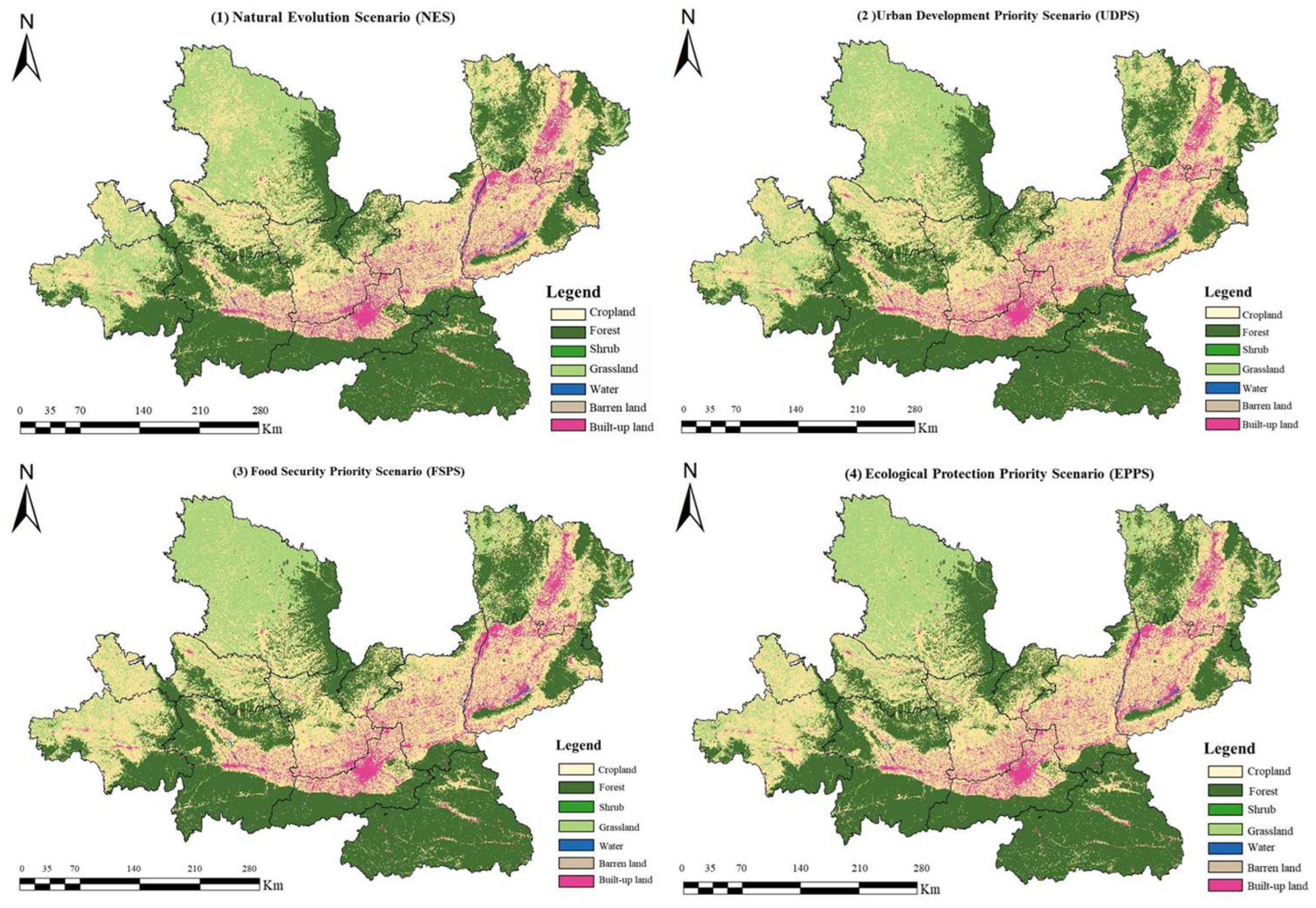
The four development scenarios demonstrate pronounced spatial heterogeneity in their outcomes, as shown in Figure 16. Under the Natural Evolution Scenario, urban expansion primarily manifests along existing transportation corridors, creating a dispersed development pattern that reflects market-driven forces without policy intervention. This scenario projects built-up land expansion following historical trends, with development occurring predominantly in areas with favorable accessibility and topographic conditions. The spatial distribution reveals continued encroachment of urban areas into agricultural lands, particularly in the periphery of major cities including Xi’an, Xianyang, and Weinan.
The Urban Development Priority Scenario facilitates more concentrated urban morphology through strategic policy interventions that promote compact development. Built-up areas demonstrate enhanced clustering patterns, concentrating toward regions with superior transportation infrastructure and gentle topography. This scenario achieves greater spatial efficiency by directing development toward designated growth zones while maintaining agricultural productivity in protected areas. The resulting urban form exhibits higher density characteristics with reduced spatial fragmentation compared to natural evolution patterns.
The Food Security Priority Scenario implements stringent protection measures for prime agricultural lands, fundamentally altering spatial development trajectories. High-quality cropland in plain areas receives comprehensive protection, redirecting urban expansion toward less agriculturally productive hilly and piedmont zones. This spatial reallocation demonstrates the policy’s effectiveness in preserving food production capacity while accommodating necessary urban growth. The scenario reveals how agricultural protection policies can reshape regional development patterns by channeling urbanization toward marginal lands.
The Ecological Protection Priority Scenario achieves the most environmentally sustainable spatial configuration through comprehensive ecological constraints and restoration initiatives. This scenario produces the most compact urban layout with built-up land area minimized to 10,410 km2, representing the smallest urban footprint among all scenarios. Simultaneously, ecological spaces receive enhanced protection and expansion, with forest areas achieving maximum coverage. The spatial pattern demonstrates successful integration of urban development needs with ecological preservation objectives.
Regional development impacts exhibit considerable spatial variation across scenarios. The Xi’an–Xianyang metropolitan core experiences rapid urbanization under all scenarios, though expansion intensities differ substantially. The Urban Development Priority Scenario generates maximum built-up land increment in this region, while the Ecological Protection Priority Scenario produces the most restrained growth. Agricultural production regions including Weinan and Yuncheng demonstrate optimal farmland conservation under the Food Security Priority Scenario, contrasting sharply with substantial conversion pressures experienced under urban-oriented development policies. Mountainous cities such as Shangluo and Tianshui exhibit relatively modest variations across scenarios due to inherent topographic limitations that constrain development options regardless of policy framework.

5. Discussion

5.1. Complex System Characteristics and Theoretical Contributions of PLE Space Evolution

This investigation illuminates the fundamental nature of PLE space evolution through a complex systems theoretical lens, revealing that spatial transformation in the Guanzhong Plain Urban Agglomeration constitutes a nonlinear dynamic process characterized by threshold effects and emergent properties rather than simple linear progression. The phenomenon whereby grassland-to-forest transitions achieved absolute tendency during 2016–2021 exemplifies ecosystem self-organization capacity under policy guidance and demonstrates systemic phase transitions within socio-ecological systems [87].
The identification of temporal lag effects between policy implementation and spatial response reveals critical insights into policy-space dynamics. National policy interventions do not immediately manifest in spatial configurations but require approximately 3–5 years for transmission and materialization in landscape patterns [88]. This temporal disconnection provides essential guidance for policy evaluation frameworks: assessments of policy effectiveness must incorporate sufficient temporal windows to avoid premature policy adjustments based on short-term observable outcomes.
The driving mechanism analysis transcends traditional single-factor explanatory models, establishing a multi-factor coupling framework that acknowledges system complexity [89]. The foundational role of environmental factors (45–55% contribution) confirms natural geographic conditions as fundamental constraints in spatial pattern formation, while the spatiotemporally heterogeneous influences of socioeconomic factors demonstrate greater complexity. Population density’s decisive influence on living space expansion (24.2% contribution) validates the centrality of demographic agglomeration in urbanization theory, whereas the differentiated impacts of economic development across various space types reflect the selective role of market mechanisms in spatial resource allocation.
The nonlinear characteristics of spatial evolution challenge conventional planning paradigms predicated on linear causality. The identification of threshold effects—particularly the constraint of population-driven urban expansion above 1000 m elevation—and complex interactions among multiple drivers necessitate sophisticated analytical frameworks capable of capturing system dynamics beyond simple cause-effect relationships. These findings establish the theoretical foundation for adaptive governance approaches that acknowledge uncertainty and complexity rather than pursuing deterministic control.

5.2. Decision Support Value and Policy Implications of Multi-Scenario Analysis

Scenario analysis emerges as a critical prospective research methodology for decision support under conditions of deep uncertainty and complexity [90]. The four-scenario framework developed in this study not only evaluates spatial consequences of different policy orientations but, more significantly, reveals unavoidable trade-offs inherent in sustainable development processes.
The core finding of trade-off analysis demonstrates that any single-objective policy orientation generates negative externalities across other dimensions. Urban development prioritization maximizes economic benefits while incurring 15.4% ecological space losses; ecological protection prioritization achieves optimal environmental outcomes while potentially constraining regional development vitality [91]. This revelation provides crucial warnings for decision-makers: the illusion of “perfect solutions” must be abandoned in favor of trade-off-based adaptive governance approaches [92].
The proposition of spatially differentiated governance strategies offers substantial practical guidance. The implementation of food security priorities in plain agricultural areas, ecological protection priorities in mountainous regions, and urban development priorities in metropolitan cores embodies precision governance principles of “one place, one policy” [93]. This strategic differentiation not only acknowledges comparative advantages across different geographical zones but achieves coordinated regional development through functional specialization.
The design of temporal coordination mechanisms provides approaches for resolving spatiotemporal conflicts between development and conservation. The strategy of short-term prioritization of ecological restoration and food security assurance, with gradual long-term release of development space, reflects the unification of intergenerational equity and developmental stage considerations in sustainable development [94]. This temporal arrangement maintains regional ecological security baselines while preserving space for future development opportunities.
The inter-regional coordination framework addresses uneven development impacts through market-based mechanisms. Ecological compensation systems and development rights trading mechanisms create economic incentives for environmental protection while maintaining regional balance, offering potential solutions to spatial allocation challenges revealed through scenario analysis [95].

5.3. Research Limitations and Future Directions

Despite methodological innovations and empirical advances, this study acknowledges several limitations requiring future research attention and refinement.
At the data and methodological level, static driving factor treatment may underestimate dynamic process influences. Climate change as a slow variable affecting long-term spatial patterns, technological advancement enhancing land use efficiency, and policy evolution guiding spatial allocation all require consideration within dynamic frameworks [96]. Future research should develop time-varying parameter models to better capture dynamic characteristics of driving factors.
Scenario design limitations primarily manifest in inadequate uncertainty treatment. Real-world “black swan” events—including sudden crises, technological breakthroughs, and social transformations—may fundamentally alter spatial evolution trajectories [97], yet existing scenario frameworks cannot encompass all possibilities. Future research should incorporate Monte Carlo simulation, fuzzy set theory, and other methodologies to enhance uncertainty-handling capabilities in scenario analysis.
Research scope limitations concern representativeness of single case studies. While the Guanzhong Plain Urban Agglomeration represents a typical western region case, the applicability of conclusions to eastern developed regions, northeastern industrial bases, and southwestern mountainous areas requires verification [98]. Multi-case comparative studies should identify universal patterns and context-specific manifestations of PLE space evolution across different development stages and geographical environments.
The specific geographical context of the Guanzhong Plain—characterized by a semi-arid climate, topographical constraints with the Qinling Mountains to the south and the Loess Plateau to the north, and distinct policy legacies as a historical development priority area in western China—shapes the observed patterns of PLE space evolution. The dominance of environmental factors (45–55% contribution) and the identified elevation threshold effects (particularly the 1000 m constraint on urban expansion) are closely tied to this mountainous-basin topography. Similarly, the 3–5-year policy transmission lag may reflect institutional characteristics specific to China’s multi-level governance system. Therefore, caution must be exercised when extrapolating these findings to regions with fundamentally different physical geographies (e.g., coastal plains, tropical environments), economic development stages (e.g., post-industrial metropolises), or institutional arrangements (e.g., market-driven land use systems in developed countries). Comparative studies across diverse geographical and institutional contexts are essential to distinguish universal mechanisms of PLE space evolution from context-dependent manifestations.
Theoretical expansion requires deeper integration of PLE space theory with related theoretical frameworks. Integration with landscape ecology’s scale theory, economic geography’s spatial structure theory, and sociology’s spatial production theory would contribute to more comprehensive spatial evolution theoretical systems [99]. Additionally, international comparative studies should explore PLE space theory adaptability under different institutional environments and development models [100].

6. Conclusions

This study provides a comprehensive analysis of Production-Living-Ecological space evolution in the Guanzhong Plain Urban Agglomeration from 2001 to 2021, employing an integrated framework combining multiple spatial analysis methods, machine learning algorithms, and scenario simulation techniques. The findings offer crucial insights for sustainable spatial planning in rapidly urbanizing regions facing complex trade-offs between development and conservation. Four main conclusions emerge from this research:
(1)
PLE space evolution in the GPUA exhibits distinct stage characteristics with significant spatial restructuring. Living space expanded by 73.89% while production and ecological spaces contracted by 7.47% and 8.94%, respectively, over the 20-year period. The evolution process displayed four distinct phases—rapid expansion (2001–2006), structural adjustment (2006–2011), quality improvement (2011–2016), and green transformation (2016–2021)—each corresponding to national policy shifts but manifesting with regional time lags. The divergent migration trajectories of PLE space gravity centers (production space shifting 23.4 km southwest, ecological space moving 18.9 km northwest, living space remaining stable) reveal the asymmetric nature of regional development and the persistence of established urban hierarchies despite rapid transformation.
(2)
Driving mechanisms of PLE space evolution demonstrate complex nonlinear relationships and strong scale dependencies. Environmental factors (precipitation, temperature, elevation) establish the fundamental template for spatial patterns, contributing 45–55% of explanatory power. However, their influence varies significantly across space types and geographic regions—economic factors dominate in plains (>40% contribution), environmental factors prevail in mountains (>60%), and social factors peak in peri-urban zones (35–45%). The identification of threshold effects (e.g., elevation’s constraint on population-driven urban expansion above 1000 m) and interaction effects among multiple drivers challenges linear conceptualizations of land use change and highlights the need for sophisticated analytical approaches to capture system complexity.
(3)
Multi-scenario simulations reveal inevitable trade-offs but also optimization possibilities through strategic spatial planning. No single development pathway can simultaneously maximize all PLE space functions—urban development scenarios achieve 55.34% built-up land expansion but sacrifice agricultural and ecological integrity, while conservation scenarios preserve ecosystem services but constrain economic growth potential. However, the ecological protection scenario demonstrates that careful spatial allocation can achieve 92% of baseline food production capacity while maintaining the highest ecological connectivity (0.63) and carbon storage (1287 Mt C), suggesting that integrated planning approaches can partially reconcile competing objectives. These findings emphasize the necessity of explicit priority-setting and differentiated strategies tailored to regional contexts rather than uniform policy applications.
(4)
The integrated Markov chain-PLUS modeling framework advances land use simulation methodology and provides robust decision support for sustainable development. The coupled approach achieved exceptional validation accuracy (Kappa = 0.91), demonstrating its reliability for policy-relevant projections. By combining quantity projection with spatial allocation, incorporating machine learning for driver identification, and enabling multi-scenario exploration, the framework addresses key limitations of existing models while maintaining computational efficiency. Beyond methodological contributions, this study provides actionable insights for the GPUA’s sustainable development: core metropolitan areas should prioritize compact development, agricultural zones require consolidated protection with modernization, and ecological areas need integrated conservation with community welfare. These differentiated strategies, implemented through adaptive governance mechanisms, can guide the region toward a more sustainable spatial configuration that balances economic prosperity, food security, and ecological integrity in the face of continued urbanization pressure.

Author Contributions

Conceptualization, S.L. and H.B.; methodology, C.G.; software, C.G.; validation, S.L., H.B. and C.G.; formal analysis, S.L. and C.G.; investigation, S.L. and C.G.; resources, H.B. and C.G.; data curation, C.G.; writing—original draft preparation, S.L. and C.G.; writing—review and editing, S.L.; visualization, C.G.; supervision, C.G.; project administration, Y.Z.; funding acquisition, S.L. and C.G. All authors have read and agreed to the published version of the manuscript.

Funding

This research was funded by the National statistical science research project, grant number 2025LY022 and Fundamental Research Funds for the Central Universities, grant number 300102115602.

Data Availability Statement

The raw data supporting the conclusions of this article will be made available by the authors on request.

Conflicts of Interest

The authors declare no conflicts of interest.

References

  1. Seto, K.C.; Güneralp, B.; Hutyra, L.R. Global Forecasts of Urban Expansion to 2030 and Direct Impacts on Biodiversity and Carbon Pools. Proc. Natl. Acad. Sci. USA 2012, 109, 16083–16088. [Google Scholar] [CrossRef]
  2. United Nations Department of Economic and Social Affairs. World Urbanization Prospects: The 2018 Revision; United Nations: New York, NY, USA, 2019; ISBN 978-92-1-004314-4. [Google Scholar]
  3. Bibi, S.; Duclos, J.-Y. L’effet des prélèvements fiscaux et des transferts aux particuliers sur la pauvreté au Québec et au Canada. Can. Public Policy 2011, 37, 1–24. [Google Scholar] [CrossRef]
  4. Li, Y.; Zhao, J.; Zhang, S.; Zhang, G.; Zhou, L. Qualitative-Quantitative Identification and Functional Zoning Analysis of Production-Living-Ecological Space: A Case Study of Urban Agglomeration in Central Yunnan, China. Environ. Monit. Assess. 2023, 195, 1163. [Google Scholar] [CrossRef] [PubMed]
  5. Wang, Q.; Wang, H.; Zeng, H.; Chang, R.; Bai, X. Understanding Relationships between Landscape Multifunctionality and Land-Use Change across Spatiotemporal Characteristics: Implications for Supporting Landscape Management Decisions. J. Clean. Prod. 2022, 377, 134474. [Google Scholar] [CrossRef]
  6. Lee, E.; Kim, G. Analysis of Domestic and International Green Infrastructure Research Trends from the ESG Perspective in South Korea. Int. J. Environ. Res. Public Health 2022, 19, 7099. [Google Scholar] [CrossRef] [PubMed]
  7. Padró, R.; La Rota-Aguilera, M.J.; Giocoli, A.; Cirera, J.; Coll, F.; Pons, M.; Pino, J.; Pili, S.; Serrano, T.; Villalba, G.; et al. Assessing the Sustainability of Contrasting Land Use Scenarios through the Socioecological Integrated Analysis (SIA) of the Metropolitan Green Infrastructure in Barcelona. Landsc. Urban Plan. 2020, 203, 103905. [Google Scholar] [CrossRef]
  8. Fernández-Martínez, M.; Janssens, I.A.; Obersteiner, M.; Manning, P.; Andrade, F.M.; Rodríguez-Penedo, E.; Peñuelas, J. Temporal Complexity of Terrestrial Ecosystem Functioning and Its Drivers. Nat. Commun. 2025, 16, 7725. [Google Scholar] [CrossRef]
  9. Su, N.; Tang, R.; Zhang, Y.; Ni, J.; Huang, Y.; Liu, C.; Xiao, Y.; Zhu, B.; Zhao, Y. Using Machine Learning to Identify Risk Factors for Pancreatic Cancer: A Retrospective Cohort Study of Real-World Data. Front. Pharmacol. 2024, 15, 1510220. [Google Scholar] [CrossRef]
  10. Antonelli, G.; Puddu, G.; Cipollini, C.; Sabatini, G.; Conticelli, M.; Simeone, M.C. A Vanishing Imprint? Modeling the Present and Future Distribution of the Enigmatic Quercus Crenata Lam., a Mediterranean Sporadic Tree Species. Ecol. Evol. 2025, 15, e71482. [Google Scholar] [CrossRef]
  11. Ye, H.; Song, Y.; Xue, D. Multi-Scenario Simulation of Land Use and Habitat Quality in the Guanzhong Plain Urban Agglomeration, China. Int. J. Environ. Res. Public Health 2022, 19, 8703. [Google Scholar] [CrossRef]
  12. Gentine, P.; Alemohammad, S.H. Reconstructed Solar-Induced Fluorescence: A Machine Learning Vegetation Product Based on MODIS Surface Reflectance to Reproduce GOME-2 Solar-Induced Fluorescence. Geophys. Res. Lett. 2018, 45, 3136–3146. [Google Scholar] [CrossRef]
  13. Ye, Y.; Pandey, A.; Bawden, C.; Sumsuzzman, D.M.; Rajput, R.; Shoukat, A.; Singer, B.H.; Moghadas, S.M.; Galvani, A.P. Integrating Artificial Intelligence with Mechanistic Epidemiological Modeling: A Scoping Review of Opportunities and Challenges. Nat. Commun. 2025, 16, 581. [Google Scholar] [CrossRef]
  14. Han, L.; Qin, T.; Sun, Z.; Ren, H.; Zhao, N.; An, X.; Wang, Z. Influence of Urbanization on the Spatial Distribution of Associations Between Air Pollution and Mortality in Beijing, China. GeoHealth 2023, 7, e2022GH000749. [Google Scholar] [CrossRef]
  15. Iglesias-Carrasco, M.; Medina, I.; Ord, T.J. Global Effects of Forest Modification on Herpetofauna Communities. Conserv. Biol. 2023, 37, e13998. [Google Scholar] [CrossRef] [PubMed]
  16. Elum, Z.A.; Mopipi, K.; Henri-Ukoha, A. Oil Exploitation and Its Socioeconomic Effects on the Niger Delta Region of Nigeria. Environ. Sci. Pollut. Res. 2016, 23, 12880–12889. [Google Scholar] [CrossRef]
  17. Liu, X.; Wei, M.; Zeng, J. Simulating Urban Growth Scenarios Based on Ecological Security Pattern: A Case Study in Quanzhou, China. Int. J. Environ. Res. Public Health 2020, 17, 7282. [Google Scholar] [CrossRef] [PubMed]
  18. Xu, C.; Xie, D.; Gu, C.; Zhao, P.; Wang, X.; Wang, Y. Sustainable Development Pathways for Energies in Yangtze River Delta Urban Agglomeration. Sci. Rep. 2023, 13, 18135. [Google Scholar] [CrossRef]
  19. Severo, E.A.; De Guimarães, J.C.F.; Dellarmelin, M.L. Impact of the COVID-19 Pandemic on Environmental Awareness, Sustainable Consumption and Social Responsibility: Evidence from Generations in Brazil and Portugal. J. Clean. Prod. 2021, 286, 124947. [Google Scholar] [CrossRef]
  20. López, D.; Sáez, P.L.; Cavieres, L.A.; Beveridge, F.C.; Saavedra-Mella, F.; Bravo, L.A. Morpho-Physiological Traits and Dehydration Tolerance of High-Altitude Andean Wetland Vegetation in the Chilean Atacama Region. Plant-Environ. Interact. 2025, 6, e70038. [Google Scholar] [CrossRef]
  21. Yang, G.; Liu, Y.; Wen, S.; Chen, W.; Zhu, X.; Wang, Y. DTI-MHAPR: Optimized Drug-Target Interaction Prediction via PCA-Enhanced Features and Heterogeneous Graph Attention Networks. BMC Bioinform. 2025, 26, 11. [Google Scholar] [CrossRef]
  22. Marrec, R.; Abdel Moniem, H.E.; Iravani, M.; Hricko, B.; Kariyeva, J.; Wagner, H.H. Conceptual Framework and Uncertainty Analysis for Large-Scale, Species-Agnostic Modelling of Landscape Connectivity across Alberta, Canada. Sci. Rep. 2020, 10, 6798. [Google Scholar] [CrossRef]
  23. Zhang, D.; Wang, J.; Wang, Y.; Xu, L.; Zheng, L.; Zhang, B.; Bi, Y.; Yang, H. Is There a Spatial Relationship between Urban Landscape Pattern and Habitat Quality? Implication for Landscape Planning of the Yellow River Basin. Int. J. Environ. Res. Public Health 2022, 19, 11974. [Google Scholar] [CrossRef] [PubMed]
  24. Sriver, R.L.; Lempert, R.J.; Wikman-Svahn, P.; Keller, K. Characterizing Uncertain Sea-Level Rise Projections to Support Investment Decisions. PLoS ONE 2018, 13, e0190641. [Google Scholar] [CrossRef]
  25. Simkin, S.; Chamberland-Rowe, C.; Damba, C.; Sava, N.; Lim, T.; Bourgeault, I.L. Implementing Leading Practices in Regional-Level Primary Care Workforce Planning: Lessons Learned in Toronto. Healthc. Manag. Forum 2023, 36, 15–20. [Google Scholar] [CrossRef] [PubMed]
  26. Thiault, L.; Mora, C.; Cinner, J.E.; Cheung, W.W.L.; Graham, N.A.J.; Januchowski-Hartley, F.A.; Mouillot, D.; Sumaila, U.R.; Claudet, J. Escaping the Perfect Storm of Simultaneous Climate Change Impacts on Agriculture and Marine Fisheries. Sci. Adv. 2019, 5, eaaw9976. [Google Scholar] [CrossRef] [PubMed]
  27. Yao, L.; Halike, A.; Yao, K.; Wei, Q.; Tang, H.; Tuheti, B.; Luo, J.; Duan, Y. Dynamic Simulation of Landscape Ecological Security and Analysis of Coupling Coordination Degree: A Case Study of Bole. PLoS ONE 2024, 19, e0297860. [Google Scholar] [CrossRef]
  28. Li, Y.; Beeton, R.J.S.; Sigler, T.; Halog, A. Enhancing the Adaptive Capacity for Urban Sustainability: A Bottom-up Approach to Understanding the Urban Social System in China. J. Environ. Manag. 2019, 235, 51–61. [Google Scholar] [CrossRef]
  29. Li, Y.; Xie, H. Spatial–Temporal Variation and Correlation Analysis of Ecosystem Service Values and Ecological Risks in Winter City Shenyang, China. Sci. Rep. 2024, 14, 18182. [Google Scholar] [CrossRef]
  30. Zhang, H.; Yang, Q.; Zhang, Z.; Lu, D.; Zhang, H. Spatiotemporal Changes of Ecosystem Service Value Determined by National Land Space Pattern Change: A Case Study of Fengdu County in The Three Gorges Reservoir Area, China. Int. J. Environ. Res. Public Health 2021, 18, 5007. [Google Scholar] [CrossRef]
  31. Lemiere, L.; Jaeger, M.; Gosme, M.; Subsol, G. Combinatorial Maps, a New Framework to Model Agroforestry Systems. Plant Phenomics 2023, 5, 0120. [Google Scholar] [CrossRef]
  32. Brandt, J. Multifunctional Landscapes—Perspectives for the Future. J. Environ. Sci. 2003, 15, 187–192. [Google Scholar]
  33. Sun, H.; Cheng, L.; Li, Z.; Wang, Q.; Teng, J. A Land-Use Benefit Evaluation System with Case Study Verification. PLoS ONE 2022, 17, e0271557. [Google Scholar] [CrossRef]
  34. Hansen, R.; Pauleit, S. From Multifunctionality to Multiple Ecosystem Services? A Conceptual Framework for Multifunctionality in Green Infrastructure Planning for Urban Areas. AMBIO 2014, 43, 516–529. [Google Scholar] [CrossRef]
  35. Luo, K.; Wang, H.; Ma, C.; Wu, C.; Zheng, X.; Xie, L. Carbon Sinks and Carbon Emissions Balance of Land Use Transition in Xinjiang, China: Differences and Compensation. Sci. Rep. 2022, 12, 22456. [Google Scholar] [CrossRef]
  36. Xu, H.; Zhang, F.; Li, W.; Shi, J.; Johnson, B.A.; Tan, M.L. Spatial-Temporal Pattern of Change in Production-Living-Ecological Space of Nanchong City from 2000 to 2020 and Underlying Factors. Environ. Monit. Assess. 2023, 196, 94. [Google Scholar] [CrossRef] [PubMed]
  37. Tabatabaei Hosseini, S.A.; Kazemzadeh, R.; Foster, B.J.; Arpali, E.; Süsal, C. New Tools for Data Harmonization and Their Potential Applications in Organ Transplantation. Transplantation 2024, 108, 2306–2317. [Google Scholar] [CrossRef] [PubMed]
  38. Welch, H.; Brodie, S.; Jacox, M.G.; Bograd, S.J.; Hazen, E.L. Decision-support Tools for Dynamic Management. Conserv. Biol. 2020, 34, 589–599. [Google Scholar] [CrossRef] [PubMed]
  39. McMahon, S.; Matzke, M.; Tuni, C. Food Limitation but Not Enhanced Rates of Ejaculate Production Imposes Reproductive and Survival Costs to Male Crickets. Cells 2021, 10, 1498. [Google Scholar] [CrossRef]
  40. Johnson, A.H.; Harrison, T.C. Advanced Practice Registered Nurse Transition to Practice in the Long-Term Care Setting: An Ethnography. Glob. Qual. Nurs. Res. 2022, 9, 23333936221108701. [Google Scholar] [CrossRef]
  41. Stephanou, C.; Omirou, M.; Philippot, L.; Zissimos, A.M.; Christoforou, I.C.; Trajanoski, S.; Oulas, A.; Ioannides, I.M. Land Use in Urban Areas Impacts the Composition of Soil Bacterial Communities Involved in Nitrogen Cycling. A Case Study from Lefkosia (Nicosia) Cyprus. Sci. Rep. 2021, 11, 8198. [Google Scholar] [CrossRef]
  42. Khadka, D.; Babel, M.S.; Tingsanchali, T.; Penny, J.; Djordjevic, S.; Abatan, A.A.; Giardino, A. Evaluating the Impacts of Climate Change and Land-Use Change on Future Droughts in Northeast Thailand. Sci. Rep. 2024, 14, 9746. [Google Scholar] [CrossRef]
  43. Li, Y.; Ma, Y.; Liu, J.; Yang, J. Analysis of the Spatial and Temporal Evolution of Urban Resilience in Four Southern Regions of Xinjiang. Int. J. Environ. Res. Public Health 2023, 20, 5106. [Google Scholar] [CrossRef] [PubMed]
  44. Simon, F.; Gironás, J.; Rivera, J.; Vega, A.; Arce, G.; Molinos-Senante, M.; Jorquera, H.; Flamant, G.; Bustamante, W.; Greene, M.; et al. Toward Sustainability and Resilience in Chilean Cities: Lessons and Recommendations for Air, Water, and Soil Issues. Heliyon 2023, 9, e18191. [Google Scholar] [CrossRef] [PubMed]
  45. Schebella, M.F.; Weber, D.; Schultz, L.; Weinstein, P. The Nature of Reality: Human Stress Recovery during Exposure to Biodiverse, Multisensory Virtual Environments. Int. J. Environ. Res. Public Health 2020, 17, 56. [Google Scholar] [CrossRef] [PubMed]
  46. Erb, K.H. How a Socio-Ecological Metabolism Approach Can Help to Advance Our Understanding of Changes in Land-Use Intensity. Ecol. Econ. 2012, 76, 8–14. [Google Scholar] [CrossRef]
  47. Dabinett, G. Spatial Justice and the Translation of European Strategic Planning Ideas in the Urban Sub-Region of South Yorkshire. Urban Stud. 2010, 47, 2389–2408. [Google Scholar] [CrossRef]
  48. Liu, L.; Tian, Y. Does the Compact City Paradigm Help Reduce Poverty? Evidence from China. Int. J. Environ. Res. Public Health 2022, 19, 6184. [Google Scholar] [CrossRef]
  49. Xu, N.; Chen, W.; Pan, S.; Liang, J.; Bian, J. Evolution Characteristics and Formation Mechanism of Production-Living-Ecological Space in China: Perspective of Main Function Zones. Int. J. Environ. Res. Public Health 2022, 19, 9910. [Google Scholar] [CrossRef]
  50. Obersteiner, M.; Walsh, B.; Frank, S.; Havlík, P.; Cantele, M.; Liu, J.; Palazzo, A.; Herrero, M.; Lu, Y.; Mosnier, A.; et al. Assessing the Land Resource–Food Price Nexus of the Sustainable Development Goals. Sci. Adv. 2016, 2, e1501499. [Google Scholar] [CrossRef]
  51. Chi, G.; Wang, D. Population Projection Accuracy: The Impacts of Sociodemographics, Accessibility, Land Use, and Neighbour Characteristics. Popul. Space Place 2018, 24, e2129. [Google Scholar] [CrossRef]
  52. Ngouhouo-Poufoun, J.; Chaupain-Guillot, S.; Ndiaye, Y.; Sonwa, D.J.; Njabo, K.Y.; Delacote, P. Cocoa, Livelihoods, and Deforestation within the Tridom Landscape in the Congo Basin: A Spatial Analysis. PLoS ONE 2024, 19, e0302598. [Google Scholar] [CrossRef]
  53. Luan, C.; Liu, R.; Zhang, Q.; Sun, J.; Liu, J. Multi-objective land use optimization based on integrated NSGA–II–PLUS model: Comprehensive consideration of economic development and ecosystem services value enhancement. J. Clean. Prod. 2024, 434, 140306. [Google Scholar] [CrossRef]
  54. Jakovac, C.C.; Dutrieux, L.P.; Siti, L.; Peña-Claros, M.; Bongers, F. Spatial and Temporal Dynamics of Shifting Cultivation in the Middle-Amazonas River: Expansion and Intensification. PLoS ONE 2017, 12, e0181092. [Google Scholar] [CrossRef] [PubMed]
  55. Kariuki, R.W.; Munishi, L.K.; Courtney-Mustaphi, C.J.; Capitani, C.; Shoemaker, A.; Lane, P.J.; Marchant, R. Integrating Stakeholders’ Perspectives and Spatial Modelling to Develop Scenarios of Future Land Use and Land Cover Change in Northern Tanzania. PLoS ONE 2021, 16, e0245516. [Google Scholar] [CrossRef] [PubMed]
  56. Dai, E.; Wu, S.; Shi, W.; Cheung, C.; Shaker, A. Modeling Change-Pattern-Value Dynamics on Land Use: An Integrated GIS and Artificial Neural Networks Approach. Environ. Manag. 2005, 36, 576–591. [Google Scholar] [CrossRef]
  57. Guo, L.; Liu, Y.; Jiang, Z.; Yuan, X.; Jing, Q. Impact of Land Prices on Corporate Carbon Emission Intensity. Sci. Rep. 2025, 15, 3632. [Google Scholar] [CrossRef]
  58. Sellers, S.; Bilsborrow, R.; Salinas, V.; Mena, C. Population and Development in the Amazon: A Longitudinal Study of Migrant Settlers in the Northern Ecuadorian Amazon. Acta Amaz. 2017, 47, 321–330. [Google Scholar] [CrossRef]
  59. Shi, Y.; Zhu, Q.; Xu, L.; Lu, Z.; Wu, Y.; Wang, X.; Fei, Y.; Deng, J. Independent or Influential? Spatial-Temporal Features of Coordination Level between Urbanization Quality and Urbanization Scale in China and Its Driving Mechanism. Int. J. Environ. Res. Public Health 2020, 17, 1587. [Google Scholar] [CrossRef]
  60. Qiu, J.; Game, E.T.; Tallis, H.; Olander, L.P.; Glew, L.; Kagan, J.S.; Kalies, E.L.; Michanowicz, D.; Phelan, J.; Polasky, S.; et al. Evidence-Based Causal Chains for Linking Health, Development, and Conservation Actions. Bioscience 2018, 68, 182–193. [Google Scholar] [CrossRef]
  61. Corburn, J. Urban Place and Health Equity: Critical Issues and Practices. Int. J. Environ. Res. Public Health 2017, 14, 117. [Google Scholar] [CrossRef]
  62. Gao, F.; Pan, J.; Gong, Z. Detection of Spatial and Temporal Variation Characteristics of Vegetation Cover in the Lower Mekong Region and the Influencing Factors. Sci. Rep. 2024, 14, 26673. [Google Scholar] [CrossRef] [PubMed]
  63. Garzón Delvaux, P.A.; Riesgo, L.; Gomez y Paloma, S. Are Small Farms More Performant than Larger Ones in Developing Countries? Sci. Adv. 2020, 6, eabb8235. [Google Scholar] [CrossRef] [PubMed]
  64. Lu, G.; Chong, Z.; Xu, E.; Na, C.; Liu, K.; Chai, L.; Xia, P.; Yang, K.; Zhu, G.; Zhao, J.; et al. Environmental, Socioeconomic, and Sociocultural Drivers of Monkeypox Transmission in the Democratic Republic of the Congo: A One Health Perspective. Infect. Dis. Poverty 2025, 14, 7. [Google Scholar] [CrossRef] [PubMed]
  65. Devlin, L.; Goralnik, M.; Ross, W.G.; Tart, K.T. Climate Change and Public Health in North Carolina: A Unique State Offers a Unique Perspective. Environ. Health Perspect. 2014, 122, A146–A147. [Google Scholar] [CrossRef]
  66. Fan, X.; Luo, W.; Yu, H.; Rong, Y.; Gu, X.; Zheng, Y.; Ou, S.; Tiando, D.S.; Zhang, Q.; Tang, G.; et al. Landscape Evolution and Simulation of Rural Settlements around Wetland Park Based on MCCA Model and Landscape Theory: A Case Study of Chaohu Peninsula, China. Int. J. Environ. Res. Public Health 2021, 18, 13285. [Google Scholar] [CrossRef]
  67. Schneider, J.M.; Zabel, F.; Schünemann, F.; Delzeit, R.; Mauser, W. Global Cropland Could Be Almost Halved: Assessment of Land Saving Potentials under Different Strategies and Implications for Agricultural Markets. PLoS ONE 2022, 17, e0263063. [Google Scholar] [CrossRef]
  68. Wang, Y. The Impacts of Improvements in the Unified Economic and Environmental Efficiency of Transportation Infrastructure on Industrial Structure Transformation and Upgrade from the Perspective of Resource Factors. PLoS ONE 2022, 17, e0278722. [Google Scholar] [CrossRef]
  69. Liu, S.; Su, H.; Cao, G.; Wang, S.; Guan, Q. Learning from Data: A Post Classification Method for Annual Land Cover Analysis in Urban Areas. ISPRS J. Photogramm. Remote Sens. 2019, 154, 202–215. [Google Scholar] [CrossRef]
  70. Liu, J.; Liu, B.; Wu, L.; Miao, H.; Liu, J.; Jiang, K.; Ding, H.; Gao, W.; Liu, T. Prediction of Land Use for the next 30 Years Using the PLUS Model’s Multi-Scenario Simulation in Guizhou Province, China. Sci. Rep. 2024, 14, 13143. [Google Scholar] [CrossRef]
  71. Meisel, J.D.; Sarmiento, O.L.; Olaya, C.; Lemoine, P.D.; Valdivia, J.A.; Zarama, R. Towards a Novel Model for Studying the Nutritional Stage Dynamics of the Colombian Population by Age and Socioeconomic Status. PLoS ONE 2018, 13, e0191929. [Google Scholar] [CrossRef]
  72. Gulliver, J.; Morris, C.; Lee, K.; Vienneau, D.; Briggs, D.; Hansell, A. Land Use Regression Modeling to Estimate Historic (1962–1991) Concentrations of Black Smoke and Sulfur Dioxide for Great Britain. Environ. Sci. Technol. 2011, 45, 3526–3532. [Google Scholar] [CrossRef] [PubMed]
  73. Mutale, B.; Qiang, F. Modeling Future Land Use and Land Cover under Different Scenarios Using Patch-Generating Land Use Simulation Model. A Case Study of Ndola District. Front. Environ. Sci. 2024, 12, 1362666. [Google Scholar] [CrossRef]
  74. Gong, J.; Li, J.; Yang, J.; Li, S.; Tang, W. Land Use and Land Cover Change in the Qinghai Lake Region of the Tibetan Plateau and Its Impact on Ecosystem Services. Int. J. Environ. Res. Public Health 2017, 14, 818. [Google Scholar] [CrossRef] [PubMed]
  75. Shin, B.; An, G.; Cockrell, R.C. Examining B-Cell Dynamics and Responsiveness in Different Inflammatory Milieus Using an Agent-Based Model. PLoS Comput. Biol. 2024, 20, e1011776. [Google Scholar] [CrossRef]
  76. Torquato, S. Toward an Ising Model of Cancer and Beyond. Phys. Biol. 2011, 8, 015017. [Google Scholar] [CrossRef]
  77. GB/T 21010-2017; Current Land Use Classification. General Administration of Quality Supervision, Inspection and Quarantine of the People’s Republic of China: Beijing, China; Standardization Administration of China: Beijing, China, 2017.
  78. Luo, Y.; Zhang, M. Environmental Modeling and Exposure Assessment of Sediment-Associated Pyrethroids in an Agricultural Watershed. PLoS ONE 2011, 6, e15794. [Google Scholar] [CrossRef]
  79. Getis, A.; Ord, J.K. The Analysis of Spatial Association by Use of Distance Statistics. Geogr. Anal. 1992, 24, 189–206. [Google Scholar] [CrossRef]
  80. Derudder, B.; Meijers, E.; Harrison, J.; Hoyler, M.; Liu, X. Polycentric Urban Regions: Conceptualization, Identification and Implications. Reg. Stud. 2022, 56, 1–6. [Google Scholar] [CrossRef]
  81. Zhang, H.; Li, F.; Wei, S.; Jiang, L.; Xiong, J.; Zhang, T. Spatiotemporal Evolution Characteristics and Influencing Factors of Digital Industry in China. Sci. Rep. 2024, 14, 28591. [Google Scholar] [CrossRef]
  82. Pontius, R.G.; Shusas, E.; McEachern, M. Detecting Important Categorical Land Changes While Accounting for Persistence. Agric. Ecosyst. Environ. 2004, 101, 251–268. [Google Scholar] [CrossRef]
  83. Deng, X.; Huang, J.; Rozelle, S.; Uchida, E. Growth, Population and Industrialization, and Urban Land Expansion of China. J. Urban Econ. 2008, 63, 96–115. [Google Scholar] [CrossRef]
  84. Georganos, S.; Grippa, T.; Vanhuysse, S.; Lennert, M.; Shimoni, M.; Wolff, E. Very High Resolution Object-Based Land Use–Land Cover Urban Classification Using Extreme Gradient Boosting. IEEE Geosci. Remote Sens. Lett. 2018, 15, 607–611. [Google Scholar] [CrossRef]
  85. Kohavi, R. A Study of Cross-Validation and Bootstrap for Accuracy Estimation and Model Selection. In Proceedings of the 14th International Joint Conference on Artificial Intelligence, Montreal, QC, Canada, 20–25 August 1995; Volume 2, pp. 1137–1143, ISBN 978-1-55860-363-9. [Google Scholar]
  86. Oshiro, T.M.; Perez, P.S.; Baranauskas, J.A. How Many Trees in a Random Forest? In Proceedings of the Machine Learning and Data Mining in Pattern Recognition, Berlin, Germany, 13–20 July 2012; Perner, P., Ed.; Springer: Berlin/Heidelberg, Germany, 2012; pp. 154–168. [Google Scholar]
  87. Jokar Arsanjani, J.; Helbich, M.; Kainz, W.; Darvishi Boloorani, A. Integration of Logistic Regression, Markov Chain and Cellular Automata Models to Simulate Urban Expansion. Int. J. Appl. Earth Obs. Geoinf. 2013, 21, 265–275. [Google Scholar] [CrossRef]
  88. Wu, D.; Zheng, L.; Wang, Y.; Gong, J.; Li, J.; Chen, Q. Urban Expansion Patterns and Their Driving Forces Analysis: A Comparison between Chengdu-Chongqing and Middle Reaches of Yangtze River Urban Agglomerations. Environ. Monit. Assess. 2023, 195, 1121. [Google Scholar] [CrossRef] [PubMed]
  89. Aravindakshan, S.; Krupnik, T.J.; Shahrin, S.; Tittonell, P.; Siddique, K.H.M.; Ditzler, L.; Groot, J.C.J. Socio-Cognitive Constraints and Opportunities for Sustainable Intensification in South Asia: Insights from Fuzzy Cognitive Mapping in Coastal Bangladesh. Environ. Dev. Sustain. 2021, 23, 16588–16616. [Google Scholar] [CrossRef] [PubMed]
  90. Duan, Y.; Tang, J.; Li, Z.; Yang, Y.; Dai, C.; Qu, Y.; Lv, H. Optimal Planning and Management of Land Use in River Source Region: A Case Study of Songhua River Basin, China. Int. J. Environ. Res. Public Health 2022, 19, 6610. [Google Scholar] [CrossRef] [PubMed]
  91. Alanazi, M.; Alanazi, A.; Almadhor, A.; Memon, Z.A. Multiobjective Reconfiguration of Unbalanced Distribution Networks Using Improved Transient Search Optimization Algorithm Considering Power Quality and Reliability Metrics. Sci. Rep. 2022, 12, 13686. [Google Scholar] [CrossRef]
  92. Fan, C.; An, R.; Li, J.; Li, K.; Deng, Y.; Li, Y. An Approach Based on the Protected Object for Dam-Break Flood Risk Management Exemplified at the Zipingpu Reservoir. Int. J. Environ. Res. Public Health 2019, 16, 3786. [Google Scholar] [CrossRef]
  93. Hulme, P.E. Trouble on the Horizon: Anticipating Biological Invasions through Futures Thinking. Biol. Rev. 2025, 100, 461–480. [Google Scholar] [CrossRef]
  94. Gerlak, A.K.; Jacobs, K.L.; McCoy, A.L.; Martin, S.; Rivera-Torres, M.; Murveit, A.M.; Leinberger, A.J.; Thomure, T. Scenario Planning: Embracing the Potential for Extreme Events in the Colorado River Basin. Clim. Change 2021, 165, 27. [Google Scholar] [CrossRef]
  95. Palmer, A.J.; Si, L.; Tew, M.; Hua, X.; Willis, M.S.; Asseburg, C.; McEwan, P.; Leal, J.; Gray, A.; Foos, V.; et al. Computer Modeling of Diabetes and Its Transparency: A Report on the Eighth Mount Hood Challenge. Value Health 2018, 21, 724–731. [Google Scholar] [CrossRef]
  96. Wang, J.; Hu, Y.; Song, R.; Wang, W. Research on the Optimal Allocation of Ecological Land from the Perspective of Human Needs—Taking Hechi City, Guangxi as an Example. Int. J. Environ. Res. Public Health 2022, 19, 12418. [Google Scholar] [CrossRef] [PubMed]
  97. Adams, V.M.; Pressey, R.L.; Álvarez-Romero, J.G. Using Optimal Land-Use Scenarios to Assess Trade-Offs between Conservation, Development, and Social Values. PLoS ONE 2016, 11, e0158350. [Google Scholar] [CrossRef]
  98. Lana, F.C.B.; Marinho, C.C.; de Paiva, B.B.M.; Valle, L.R.; do Nascimento, G.F.; da Rocha, L.C.D.; Carneiro, M.; Batista, J.d.L.; Anschau, F.; Paraiso, P.G.; et al. Unraveling Relevant Cross-Waves Pattern Drifts in Patient-Hospital Risk Factors among Hospitalized COVID-19 Patients Using Explainable Machine Learning Methods. BMC Infect. Dis. 2025, 25, 537. [Google Scholar] [CrossRef]
  99. Chai, Y.; Hu, Y. Characteristics and Drivers of Vegetation Productivity Sensitivity to Increasing CO2 at Northern Middle and High Latitudes. Ecol. Evol. 2024, 14, e11467. [Google Scholar] [CrossRef]
  100. Reed, M.S.; Kenter, J.; Bonn, A.; Broad, K.; Burt, T.P.; Fazey, I.R.; Fraser, E.D.; Hubacek, K.; Nainggolan, D.; Quinn, C.H.; et al. Participatory Scenario Development for Environmental Management: A Methodological Framework Illustrated with Experience from the UK Uplands. J. Environ. Manag. 2013, 128, 345–362. [Google Scholar] [CrossRef]
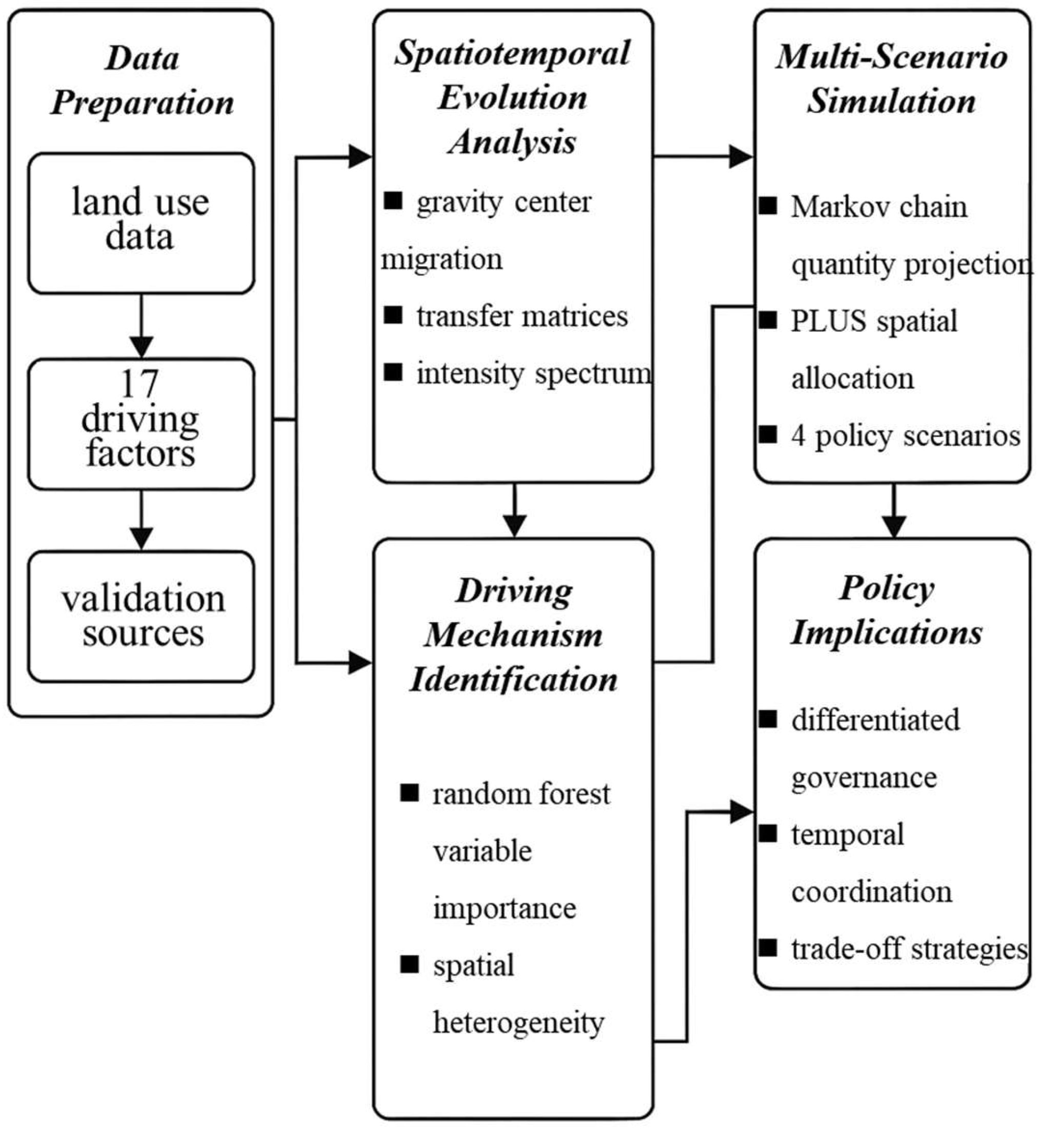
Figure 1. Integrated Research Framework and Methodological Workflow.
Land 14 02201 g001
Figure 2. Study area.
Land 14 02201 g002
Figure 3. Principles of spatial intensity map unit of land use.
Land 14 02201 g003
Figure 4. Spatial distribution of PLE spaces in the GPUA from 2001 to 2021.
Land 14 02201 g004
Figure 5. Urban built-up area evolution in the core area from 2001 to 2021. (a) Location of Xi’an Core urban Area (b) Location of Guanzhong Plain Urban Agglomeration (c) Multiphase Spatiotemporal Evolution.
Land 14 02201 g005
Figure 6. Gravity center coordinates of PLE spaces (2001–2021).
Land 14 02201 g006
Figure 7. Sankey diagram of land use transfers across different periods (2001–2021).
Land 14 02201 g007
Figure 8. Land use change intensity map for different periods: (a) 2001–2006, (b) 2006–2011, (c) 2011–2016, (d) 2016–2021. Note: Red cells represent net loss (outflow > inflow), blue cells represent net gain (inflow > outflow), with color intensity indicating magnitude of change. Light colors indicate minimal change or balance.
Land 14 02201 g008
Figure 9. Relative importance ranking of factors for cropland production space expansion.
Land 14 02201 g009
Figure 10. Relative importance ranking of factors for forest ecological space expansion.
Land 14 02201 g010
Figure 11. Relative importance ranking of factors for shrubland ecological space expansion.
Land 14 02201 g011
Figure 12. Relative importance ranking of factors for grassland ecological space expansion.
Land 14 02201 g012
Figure 13. Relative importance ranking of factors for water ecological space expansion.
Land 14 02201 g013
Figure 14. Relative importance ranking of factors for barren land ecological space expansion.
Land 14 02201 g014
Figure 15. Relative importance ranking of factors for built-up living space expansion.
Land 14 02201 g015
Figure 16. Spatial distribution patterns of PLE spaces under four scenarios for 2031.
Land 14 02201 g016
Table 1. Data sources and characteristics.
Data TypeDatasetSource/ClassificationTime
Period
Resolution
Land UseLand use
classification
China Land Cover Dataset (CLCD)2001–202130 m
Environmental Factors
Soil typeHWSD v1.2World Soil Database19951:1,000,000
Annual temperatureGPR China TempTemperature Dataset20191000 m
Annual precipitation Elevation (DEM)
NDVI
China precipitation GEBCO DEMMonthly Precipitation20191000 m
GEBCO Database2020500 m
China NDVIAnnual Vegetation Index20181000 m
Economic Factors
GDPGDP distributionChina GDP Grid Dataset20191000 m
Social Factors
PopulationWorld PopPopulation repository20201000 m
Distance to highwaysRoad networkNational Geographic Information Center/OSM20201:250,000
Distance to major roads
Distance to secondary
roads
Distance to county roads Distance to rural roads
Table 2. PLE space classification system and scoring framework.
No.Primary ClassSecondary ClassCodeProduction Space ScoreLiving Space ScoreEcological Space ScoreFinal Classification
1CroplandPaddy field11301Production
2Dry farmland12301Production
3ForestForest land21005Ecological
4Shrubland22005Ecological
5Sparse woodland23005Ecological
6Other woodland24005Ecological
7GrasslandHigh coverage31005Ecological
8Medium coverage32005Ecological
9Low coverage33005Ecological
10WaterRivers/canals41301Production
11Reservoirs/ponds Beaches43103Ecological
1246005Ecological
13Built-upUrban land51050Living
14Rural settlements52050Living
15Other construction53050Living
16UnusedSandy land61005Ecological
17Wetland64005Ecological
18Bare land66005Ecological
19Other67005Ecological
Note: Scoring scale: 0 = absent function, 1 = weak function, 3 = moderate function, 5 = prominent function. Final classification based on highest score.
Table 3. Distribution of PLE spaces across cities in 2021. Note: The orange color from deep to light is the top three changes in the same category.
CityProduction SpaceEcological SpaceLiving Space
Area (km2)% of TotalArea (km2)% of TotalArea (km2)% of Total
Xian3695.485.81%5046.045.53%1357.8819.24%
Baoji5308.928.35%12,219.2613.38%567.728.04%
Xianyang6834.3210.75%2724.132.98%766.7410.87%
Tongchuan1649.242.59%2160.872.37%86.101.22%
Weinan9063.1214.26%2762.753.03%1165.4116.51%
Shangluo2066.353.25%17,315.6718.96%162.942.31%
Tianshui6097.819.59%8021.488.78%156.892.22%
Pingliang6038.139.50%4974.925.45%105.921.50%
Qingyang5881.459.25%21,134.6923.14%84.831.20%
Yuncheng9275.4114.59%3423.993.75%1502.4721.29%
Linfen7661.3512.05%11,531.3112.63%1100.0115.59%
Table 4. Land use dynamic degrees by period (%). Note: The orange color from deep to light is the top three changes in the same category.
Land Use Spatial TypeSingle Land Use Dynamic Degree
2001~20062006~20112011~20162016~20212001~2021
Cropland Production Space−0.22%−0.71%−0.51%0.16%−1.26%
Forest Ecological Space0.79%0.66%0.54%0.67%2.78%
Shrubland Ecological Space−2.47%−7.74%−7.36%−6.22%−15.32%
Grassland Ecological Space−1.05%0.07%−0.29%−1.55%−2.72%
Water Ecological Space5.39%1.36%−0.93%2.05%8.52%
Barren Land Ecological Space−7.45%−4.65%14.61%22.37%15.30%
Built-up Living Space3.93%3.26%3.30%1.45%14.79%
Comprehensive Land Use
Dynamic Degree
0.19%0.14%0.15%0.18%0.17%
Table 5. Model Validation Metrics.
MetricValueInterpretation
Overall Accuracy92.30%Percentage of correctly classified pixels
Kappa coefficient0.91Agreement beyond chance (>0.81 = almost perfect)
Figure of Merit (FoM)0.24Ratio of correctly predicted changes to total changes
Table 6. Per-Class Validation Accuracy (%).
Land Use TypeProducer’s AccuracyUser’s Accuracy
Cropland93.291.7
Forest89.890.3
Grassland87.485.9
Built-up91.693.8
Water85.383.2
Shrubland86.784.5
Barren land88.187.3
Table 7. Land Use Demand Projections for Guanzhong Plain Urban Agglomeration (2001–2031).
YearCroplandForestShrub LandGrasslandWaterBarren LandBuilt-Up Land
200167,83750,29186434,339380814060
200667,08852,28475836,484483514854
201164,71754,00046436,591516345654
201663,06355,44629336,071492686580
202163,57457,28920233,2645421437058
202660,19661,43212230,4676131519099
203156,20461,36916729,3002653310,961
Note: Areas are expressed in square kilometers.
Table 8. Land Use Transition Parameter Settings Under Different Scenarios.
Transition TypeNatural EvolutionUrban Development PriorityFood Security PriorityEcological Protection Priority
Cropland → Built-upBaseline30%−60%−30%
Forest → Built-upBaseline20%Baseline−50%
Grassland → Built-upBaseline20%Baseline−50%
Built-up Land ConstraintsNoneNoneStrict Basic Farmland ProtectionEcological Red Line Constraints
Ecological Restoration ProbabilityBaselineBaseline10%30%
Disclaimer/Publisher’s Note: The statements, opinions and data contained in all publications are solely those of the individual author(s) and contributor(s) and not of MDPI and/or the editor(s). MDPI and/or the editor(s) disclaim responsibility for any injury to people or property resulting from any ideas, methods, instructions or products referred to in the content.