Abstract
Particulate matter (PM), particularly PM2.5, is a major urban air pollution concern globally. While temporary mitigation measures are generally implemented during high-pollution periods, sustainable solutions focusing on forest landscape management are crucial. This study examines the effects of forest landscape types and environmental variables on PM2.5 concentrations during the high-pollution period (January–March 2022) in South Korea, using data from 40 national air quality monitoring stations. GIS and Fragstats were used to construct spatial variables and landscape indices. Stepwise multiple linear regression analyses were then conducted to identify significant factors affecting PM2.5 concentrations. The aggregated forest model (i.e., without distinguishing between forest types) explained 72.9% of the variance in PM2.5 concentrations. Forest percent cover (within 5000 m) and distance from the China national border were found to negatively affect PM2.5 levels, while population size (within 5000 m) and urbanized area patch density (within 5000 m) had positive effects (p < 0.05). By incorporating forest types as variables, the forest type model improved explanatory power to 83.4%. Specifically, mixed forest percent cover (within 5000 m), mixed forest patch density (within 3000 m), and broad-leaved forest percent cover (within 1000 m) were negatively correlated with PM2.5, while population size and urbanized area patch density (within 5000 m) showed positive effects (p < 0.05). These results highlight the importance of considering forest types, along with anthropogenic environmental variables, when assessing the mitigating effects of forests on PM2.5, as both showed scale-dependent relationships with pollution levels. This study informs urban planning and long-term environmental management strategies for reducing PM2.5 pollution.
1. Introduction
Fine particulate matter (PM2.5) with an aerodynamic diameter ≤ 2.5 μm can naturally occur as yellow dust, salt particles, and pollen [1,2]. However, in urbanized and industrialized areas, it is primarily generated from anthropogenic factors [3]. These particles are mainly produced during daily activities such as vehicle exhaust, pavement, coal and oil combustion, and agricultural waste burning. Specifically, road traffic alone accounts for about 25% of ambient PM2.5 in urban areas [4], highlighting how human activities contribute to air pollution. Population growth, urbanization, and industrialization may further exacerbate this problem [5,6].
PM2.5 is a pollutant that degrades air quality, reduces visibility, and poses significant health risks. Long-term exposure to PM2.5 has been shown to increase the risk of respiratory diseases, including asthma [7] and lung cancer [8]. It also elevates mortality rates from heart attacks and strokes by 8–18% [9,10]. Furthermore, particulate matter can be adsorbed onto foliage, inhibiting plant growth and reducing maximum photosynthetic rates by up to 10–34%, which can ultimately lead to plant death [11,12]. It also has adverse socioeconomic impacts, damaging crops, tourism, and other industries [13,14,15].
The Global Agenda has set a target to reduce the annual mean PM2.5 concentration to 10 μg/m3 by 2027, and to implement effective measures to mitigate health inequalities caused by air pollution [16]. In line with this goal, policies have been implemented in the United States and South Korea, and various strategies have been developed and implemented by countries to manage and mitigate PM2.5 concentrations [17,18]. Notably, China has seen a reversal in the trend of PM2.5 levels since 2007, except for some regions affected by desert dust [19]. However, these measures focus only on controlling the sources of PM2.5 and do not address the suspended PM2.5 already present in the atmosphere [20,21]. PM2.5 can remain airborne for several days up to a week depending on meteorological conditions such as wind, humidity, and precipitation [5,22]. This emphasizes the need for planning and management measures that can sustainably reduce concentrations and mitigate suspended PM2.5 from stationary sources.
Previous research has demonstrated that PM concentrations result from a complex interaction of climatic, socioeconomic, and landscape-related factors. Meteorological conditions such as turbulence and ventilation influence how pollutants disperse through the atmosphere [23,24]. At the same time, socioeconomic elements like industrial activity, income levels, and population density are strongly associated with increased concentrations [25,26]. The structure of the landscape also plays a crucial role, with extensive and well-connected green spaces able to help reduce PM concentrations by promoting both deposition and dispersion [27,28].
Among landscape elements, forests and urban green areas have been shown to significantly reduce PM levels, with studies reporting reductions of up to 10–25% [29,30,31]. PM concentrations generally decrease from the forest edge towards the interior [32], with one study showing a sharp (~88%) decline within the first 10 m of the forest edge [33]. Furthermore, several studies have examined variations in particulate matter concentrations across different forest types [34,35] and their reduction effects in urban forests at single-tree, stand, and regional scales [36]. However, most of these studies have primarily focused on leaf-level interception and adsorption processes. Landscape ecological studies addressing land cover composition and particulate matter reduction remain relatively sparse in urban green spaces [6,36] and at the national scale [37]. Moreover, because fine particulate matter pollution is a global, transboundary issue, there is a need to investigate its dynamics across multiple geographical scales and in diverse environmental contexts [38].
This study analyzed the effects of forest types and landscape factors on PM2.5 concentrations during periods of high pollution in South Korea. By comparing an aggregated forest model (without distinguishing forest types) with a more detailed model (separating broadleaf, coniferous, and mixed forests), we assessed their multi-scale impacts on PM2.5 levels and identified other landscape features acting as sources or sinks. The findings of this study provide a scientific foundation for urban and environmental planning strategies to mitigate PM2.5 pollution.
2. Study Area, Data and Methods
2.1. Study Area
The study area is the Republic of Korea in East Asia, with a land area of 100,449 km2 and a population of 51,684,564 as of 2025 [39]. According to the Annual Report of Air Quality in Korea [40], the average PM concentration in 2023 was 37 μg/m3, with seasonal averages of 44 μg/m3 from October to April and 26 μg/m3 from June to August. From autumn to early spring (October to April), the concentration of fine particulate matter is high due to the influence of dry northwesterly winds blowing from the continent via China, while in summer (June to August), the concentration of fine particulate matter is relatively low due to the influence of southeasterly winds blowing from the sea [41]. Forests cover 63% of the country’s land area (as of 2020), with 33.4% broadleaf forests, 38.8% coniferous forests, and 27.8% mixed forests by classification [42]. The eastern part of the country is dominated by a large mountain range running north–south, while the main urban and agricultural areas are located mainly in the west. South Korea ranked 50th on the list of the most polluted countries in the world (PM2.5), with the highest share of OECD populations exposed to excessive PM2.5 [43,44].
2.2. Particulate Matter Measurement Data
Particulate matter measurement data were obtained from the National Institute of Forest Science’s air quality monitoring network [45]. PM concentrations at each site were measured using the EDM 365-SVC (GRIMM Aerosol Technik, Ainring, Germany), which determines particle size distribution and mass concentration by analyzing the light scattering of individual particles in sampled air [46,47]. The data were collected from May 2021 to April 2022 across various locations (land cover), including forests, industrial areas, residential areas, and urban areas. This study analyzed data from 40 out of the 48 measurement stations established in 2020 and 2021, excluding 8 stations located at the same site but positioned at different heights (10 m, 15 m) from the target measurement height of 5 m (Figure 1). The stations were strategically distributed to capture both forested and non-forested environments, ensuring balanced spatial coverage and providing a robust, nationally representative dataset for the objectives of this study. The PM2.5 data were pre-processed to remove missing values and outliers, identified using the 1.5 IQR method, and were subsequently aggregated into monthly mean values based on ten-minute interval measurements using Python 3.12 [48].
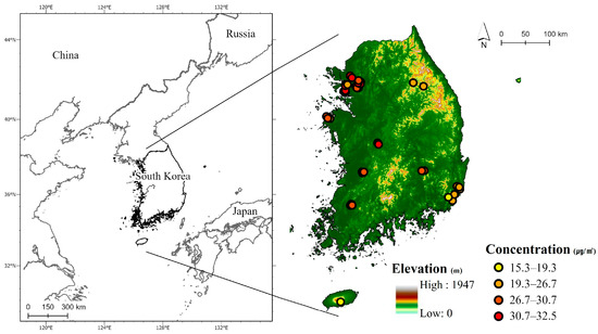
Figure 1.
Map of the study area showing the locations of PM2.5 monitoring stations and the average PM2.5 concentration from May 2021 to April 2022 (unit: μg/m3).
2.3. Methods
2.3.1. Identification of High PM2.5 Concentration Periods and Dependent Variable
High PM2.5 concentration periods were identified by analyzing the average monthly PM2.5 concentration within the study period, setting a threshold of 25 μg/m3 as the criterion for high concentration [49]. From May 2021 to April 2022, January, February, and March 2022 recorded monthly average PM2.5 concentrations exceeding 25 μg/m3 (Figure 2). Accordingly, the period from January to March 2022 was designated as the high-concentration period, and this approach was intended to represent typical PM2.5 conditions during the high-concentration season rather than short-term extreme episodes. For each monitoring station, the average PM2.5 concentration during this period was calculated and used as the dependent variable. The overall average across all stations was 28.02 μg/m3.
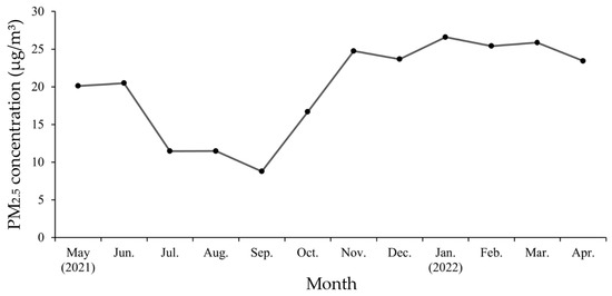
Figure 2.
Monthly average PM2.5 concentrations, based on 10 min interval data from 40 monitoring stations, were obtained for the period between May 2021 and April 2022. The high pollution period refers to the months of January to March 2022 when the monthly average concentration exceeds 25 μg/m3.
2.3.2. Independent Environmental Variables
Environmental variables were derived from spatial data measured within multiple buffer zones around the PM2.5 monitoring stations (Table 1). These variables captured landscape, urban form, socioeconomic, and geographical characteristics at multiple spatial scales.
Landscape variables included land cover composition, forest type, and major road length. For this study, the 2020 land cover map [50] was converted to a 10 m grid and classified into built-up area, broadleaf forest, coniferous forest, mixed forest, and water body. Forest classes were also aggregated into a total forest category. Using Fragstats v.4.2 [51], landscape indices were calculated for each land type at multiple scales (100, 300, 500, 1000, 2000, 3000, and 5000 m radii) around the monitoring stations. The indices included PLAND (percentage of the landscape occupied by each land type, i.e., percent cover) and PD (patch density, defined as the number of patches per hectare), which are class-level metrics demonstrated to be statistically robust and minimally redundant [52,53,54]. Road data were obtained from Geofabrik’s OpenStreetMap [55] as of May 2020. Major roads were classified as motorways and trunk roads (≥80 km/h), primary roads (≥70 km/h), and secondary roads (≥50 km/h), with buffers up to 1000 m applied based on studies showing decreasing PM2.5 concentrations with increasing distance from roads [56,57,58].
Urban form and socioeconomic variables included population, number of businesses, and official land price. Larger populations and higher land prices have been associated with higher PM2.5 concentrations [59,60], while a greater number of businesses, particularly in commercial areas, may increase PM concentrations due to reduced ventilation in dense street canyons [61,62]. Population data were obtained from the Geospatial Information Platform of National Geographic Information Institute [63], which provides 100 m resolution gridded data as of October 2020. Population size was calculated within buffer zones of 1000, 2000, and 5000 m from each monitoring site. Official land price data were also sourced from the Geospatial Information Platform, based on 100 m resolution data as of January 2021, and the mean land price (KRW/m2) of buildings was calculated within buffer zones of 100, 300, 500, 1000, 2000, 3000, and 5000 m. Business data were derived from Statistics Korea’s Statistical Geographic Information System [64], which provides 100 m resolution data as of 2019. The number of businesses was calculated within the same buffer zones.
Geographical variables included elevation with a 10 m resolution, derived from the 2019 digital topographic map at a scale of 1:5000 [63], which can influence air circulation and air quality; lower-altitude areas generally exhibited poorer air quality [65]. Distance from the China national border was also included as a geographical variable, representing the influence of transboundary PM2.5. The distance was calculated based on a map from GADM (Global Administrative Areas Database) [66]. Because national statistical datasets are updated at multi-year intervals, the most recent available values were used for each socioeconomic and land-cover variable. These indicators typically change gradually over short time periods and thus were considered acceptable proxies for conditions in early 2022.

Table 1.
Environmental variables included in regression analyses.
Table 1.
Environmental variables included in regression analyses.
| Category | Sub-Category | Abbreviation | Variable Name | Buffer Radius (m) |
|---|---|---|---|---|
| Landscape Indices [50] | Built-up area | PLAND | Bu_PLAND_radius | 100; 300; 500; 1000; 2000; 3000; 5000 |
| PD | Bu_PD_radius | |||
| Forest | PLAND | Forest_PLAND_radius | ||
| PD | Forest_PD_radius | |||
| Broad-leaved forest | PLAND | Bro_PLAND_radius | ||
| PD | Bro_PD_radius | |||
| Coniferous forest | PLAND | Con_PLAND_radius | ||
| PD | Con_PD_radius | |||
| Mixed forest | PLAND | Mix_PLAND_radius | ||
| PD | Mix_PD_radius | |||
| Water | PLAND | Water_PLAND_radius | ||
| PD | Water_PD_radius | |||
| Length of major roadways [55] | - | MR | MR_radius | 100; 200; 300; 500; 750; 1000 |
| Population size [63] | - | POP | POP_radius | 1000; 2000; 5000 |
| Number of businesses [64] | - | Count_business | Count_business _radius | 100; 300; 500; 1000; 2000; 3000; 5000 |
| Average official land price [63] | - | Mean_Land_price | Mean_Land_price _radius | |
| Elevation [63] | - | Elevation | Elevation | |
| Distance from the China national border [66] | - | Near_DIST | Near_DIST | - |
2.3.3. Forest Modeling Approaches
To evaluate the role of forests in shaping PM2.5 concentrations, two forest modeling approaches were applied: (i) an aggregated forest model using the total forest category, and (ii) a forest type model differentiating broadleaf, coniferous, and mixed forests. In both approaches, the forest variables were incorporated into the full set of independent environmental factors described in Section 2.3.2 (landscape, urban form, socioeconomic, and geographical). This design allowed us to assess whether the classification scheme of forests influenced the explanatory power of regression models.
2.3.4. Statistical Analysis
Correlation and regression analyses were conducted to identify significant environmental factors influencing PM2.5 concentrations. First, Pearson correlation analysis was performed between the dependent variable (i.e., average PM2.5 concentration during the high-concentration period) and the independent variables. To reduce multicollinearity, variables with inter-variable correlation coefficients above 0.6 were examined, and only those with stronger correlations with PM2.5 were retained, ensuring that the remaining predictors maintained coefficients below 0.6.
Stepwise multiple regression analysis using the Corrected Akaike Information Criterion (AICc) was then applied to select an appropriate PM2.5 concentration regression model. Spatial autocorrelation in the residuals was assessed using distance-based Moran’s I, and additional spatial regression models, including the spatial lag model (SLM) and the spatial error model (SEM), were implemented to assess spatial dependence. Two models (aggregated forest and forest type) were compared to assess differences in explanatory power. Statistical analyses were conducted using IBM SPSS Statistics 25 [67] and R v.4.1.3 [68].
3. Results
3.1. Correlations Between PM2.5 and Environmental Variables
Seven variables showed significant correlations with PM2.5 (|r| > 0.6; Table 2). Mixed forest percent cover within 2000–5000 m and total forest percent cover within the same range were negatively correlated with PM2.5, indicating that higher forest coverage at the landscape scale was associated with lower PM2.5 concentrations. In contrast, built-up area percent cover within 5000 m showed a positive correlation. These results suggest that both forest coverage and urbanization patterns influence PM2.5 levels. Based on the correlation analysis and considering multicollinearity, 18 variables were selected for the aggregated forest model and 21 variables for the forest type model for stepwise multiple regression analyses.
Table 2.
Pearson correlation coefficients between PM2.5 concentrations and environmental variables (|r| > 0.6, p < 0.05).
3.2. Stepwise Multiple Regression for Aggregated Forest
The stepwise multiple regression analysis incorporating aggregated forest variables explained 72.9% of the variance in PM2.5 concentrations (F = 18.25 (p < 0.001), AICc = 193.3; Table 3). Moran’s I statistics indicated weak spatial autocorrelation in the residuals, with the highest value observed at 27,500 m (I = 0.181). Furthermore, the spatial lag model (Rho = 0.00243, p = 0.979) and the spatial error model (Lambda = −0.37257, p = 0.364) were not significant, indicating that the residuals did not exhibit spatial dependence and that the multiple regression model was appropriate without spatial adjustments. In addition to the results presented in Table 3, the final model equation for the aggregated forest model is as follows:
Table 3.
Stepwise multiple regression results without distinguishing forest type.
Total forest percent cover within 5000 m and distance from the China national border were negatively associated with PM2.5, whereas population size within 5000 m and built-up area patch density within 5000 m were positively associated (p < 0.05). Additionally, built-up area percent cover within 100 m showed a marginally positive association (p = 0.051). These results indicate that landscape-scale forest coverage and transboundary PM2.5 influence local air quality, while anthropogenic factors such as the number of people and urban structure contribute to higher PM2.5 levels.
3.3. Stepwise Multiple Regression for Forest Type
When forest types were differentiated, the regression model showed higher explanatory power (R2 = 0.834, F = 34.1 (p < 0.001), AICc = 176.7; Table 4). Moran’s I statistics indicated weak spatial autocorrelation in the residuals, with the highest value observed at 1500 m (I = −0.149). The spatial lag model (Rho = −0.00033, p = 0.989) and the spatial error model (Lambda = −0.17465, p = 0.242) were not significant, indicating that the residuals did not exhibit spatial dependence and supporting the validity of the non-spatial regression model. For the forest type model, the final model equation is given below:
Table 4.
Stepwise multiple regression results with forest type variables.
Mixed forest percent cover within 5000 m, mixed forest patch density within 3000 m, and broad-leaved forest percent cover within 1000 m were negatively associated with PM2.5 concentrations, while population size within 5000 m and built-up area patch density within 5000 m were positively associated (p < 0.05). Notably, distance from the China national border was not selected as a significant variable in this model, suggesting that including forest type captured some of the variation previously explained by transboundary effects in the aggregated model.
4. Discussion
4.1. The Importance of Forest Type Classification
This study’s comparison of the aggregated forest model and the more detailed forest type model demonstrates the critical role of forest classification in explaining PM2.5 concentrations. The forest type model, with its higher explanatory power (R2 = 0.834) compared to the aggregated model (R2 = 0.729), suggests that the mitigating effect of forests on PM2.5 varies significantly by type. Consequently, a more nuanced understanding of forest composition is essential for developing accurate predictive models.
Notably, the distance from the China national border was a significant negative predictor in the aggregated model, reflecting the established influence of transboundary pollution on South Korea’s air quality [69]. However, this variable was not selected in the forest type model. This is likely because the inclusion of detailed forest type variables captured a substantial portion of the spatial variability in PM2.5, thereby reducing the explanatory contribution of the transboundary factor. This finding suggests that a detailed understanding of landscape features, particularly forest types, can provide a more comprehensive explanation of PM2.5 dynamics, even in the context of large-scale transboundary pollution. To build on this, future research should integrate both meteorological processes and forest-landscape attributes to achieve a fuller understanding.
4.2. Forest Type and PM2.5 Mitigation Effects
Mixed forests and broad-leaved forests were found to play a significant role in reducing PM2.5 during high-pollution periods (January–March). The percent cover within 5000 m and patch density within 3000 m of mixed forests were negatively correlated with PM2.5, while the percent cover of broad-leaved forests within 1000 m also showed a negative correlation. These findings challenge the common assumption that coniferous forests, which are evergreen and dominant in Korea (38.8% of total forest cover [35]), would have the strongest winter mitigation effect. Although many broad-leaved species are deciduous, some retain foliage, and even leafless branches and bark can capture particulate matter [70]. This aligns with findings from China, where combinations of coniferous and broad-leaved forests were most effective for winter PM2.5 [34]. Collectively, these results suggest that species diversity, particularly the presence of mixed forests, is more critical than total forest area for PM2.5 mitigation.
Our results reveal a scale-dependent effect on PM2.5 mitigation. Forest mitigation of PM2.5 was more pronounced at larger spatial extents (3000–5000 m buffers) than at local scales (<1000 m). This reflects the dispersal and transport properties of PM2.5, which can remain airborne for hours to days and travel considerable distances [22]. Similar patterns have been observed in land use regression studies, where larger buffer sizes show stronger associations with landscape-level air quality than local ones [6,71]. These findings indicate that forests function not only as localized canopies but also as components of broader landscape-scale processes, where extensive and well-distributed cover contributes to improvements in air quality. While our study emphasizes large-scale effects, localized features such as urban street trees can also contribute to PM2.5 reduction by capturing pollutants near their sources, providing a complementary effect to broader landscape-scale benefits [72].
4.3. The Complex Influence of Landscape Factors
Anthropogenic landscape factors had a significant impact on PM2.5 concentrations in all our models. At the 5000 m scale, population size and built-up area patch density were positively correlated with PM2.5, reflecting the well-documented role of urbanization and associated industrial activities in aggravating air pollution [73,74]. Our findings suggest that urban sprawl may further exacerbate pollution by increasing traffic volumes and extending commuting distances, thereby generating additional vehicle emissions [75,76].
Interestingly, patch density exerted contrasting effects depending on land-cover type. For forests, higher patch density increased the amount of edge area, thereby enhancing canopy–atmosphere interactions and promoting PM2.5 adsorption. In contrast, higher patch density in built-up areas likely resulted in a wider dispersion of pollution sources, consistent with previous evidence that dispersed urban patterns are associated with elevated air pollution levels [59,77,78]. This highlights that while the same landscape index can be applied to measure fragmentation, its implications for air quality depend strongly on the underlying land cover. Taken together, these results indicate the importance of compact urban development coupled with diverse, well-distributed green spaces to maximize pollution-mitigating benefits.
Anthropogenic indicators, such as major roadway length, number of businesses, and land price, were not significant in our models. Previous research has highlighted the role of road traffic emissions in shaping PM2.5 patterns, especially near dense traffic corridors [79], and has suggested that socioeconomic indicators can act as proxies for urban activity and compactness [80]. In our study, however, these effects may have been overshadowed by population size and built-up area metrics, which more directly captured the intensity of human activities. This suggests that the relevance of specific anthropogenic indicators may vary depending on spatial scale and landscape context, emphasizing the need for careful consideration when selecting explanatory variables for urban air pollution modeling.
5. Conclusions
This study examined the effects of forest types and landscape factors on PM2.5 concentrations during a high-pollution period in South Korea. Incorporating forest type classification substantially improved the explanatory power of regression models compared to aggregated forest cover. The results demonstrate that forests act as effective sinks for PM2.5, with mixed forests and broad-leaved forests showing the strongest mitigating effects. These effects were particularly evident at larger spatial scales (3000–5000 m), highlighting that PM2.5 reduction is not merely a local canopy function but also a landscape-scale process. In contrast, anthropogenic indicators such as population size and built-up area density were consistently and positively associated with PM2.5, reflecting the contribution of urbanization to fine particulate emissions.
Long-term strategies for PM2.5 reduction should extend beyond simply increasing total forest area. Instead, they should focus on conserving and restoring diverse forest types, with a particular emphasis on mixed forests, and designing their spatial arrangement to maximize pollution-mitigating effects. Simultaneously, promoting compact urban development can help reduce emissions associated with urban sprawl. This study highlights that integrating forest composition and spatial design into environmental policy and land use planning is a crucial step toward achieving lasting reductions in particulate matter (PM2.5). While our analysis was based on standardized indicators such as cover and fragmentation, future research should incorporate additional forest attributes (e.g., density, height, health status, and stand structure) to provide a more comprehensive understanding of forest–air quality interactions and to further enhance predictive ability. In line with this focus on landscape features, this study incorporated land use and land cover (LULC) information through indices such as PLAND and PD derived from the national land cover map. Although our analyses primarily emphasized forest types, future research should integrate other LULC categories to provide a more comprehensive understanding of how diverse land-cover patterns influence PM2.5 dynamics.
Author Contributions
Conceptualization and methodology, H.N., J.J., W.K. and C.-R.P.; data curation, H.N. and J.J.; formal analysis, H.N., J.J. and W.K.; investigation and visualization, H.N., J.J. and W.K.; funding acquisition, project administration, and resources, W.K. and C.-R.P.; supervision, W.K. and C.-R.P.; writing—original draft preparation, H.N., J.J. and W.K.; validation and writing—review and editing, H.N., J.J., W.K. and C.-R.P. All authors have read and agreed to the published version of the manuscript.
Funding
This work was supported by the National Institute of Forest Science (NIFoS) of Korea (Project No. FM0500-2022-01-2025).
Data Availability Statement
Data supporting the findings of this study can be provided upon reasonable request to the corresponding author.
Acknowledgments
We would like to thank the anonymous reviewers for their helpful comments.
Conflicts of Interest
Author Jina Jeong was employed by Creative & Communications Consulting Company. The remaining authors declare that the research was conducted in the absence of any commercial or financial relationships that could be construed as a potential conflict of interest.
References
- Birmili, W.; Schepanski, K.; Ansmann, A.; Spindler, G.; Tegen, I.; Wehner, B.; Nowak, A.; Reimer, E.; Mattis, I.; Müller, K.J.A.C.; et al. A Case of Extreme Particulate Matter Concentrations over Central Europe Caused by Dust Emitted over the Southern Ukraine. Atmos. Chem. Phys. 2008, 8, 997–1016. [Google Scholar] [CrossRef]
- Perrino, C.; Canepari, S.; Catrambone, M.; Dalla Torre, S.; Rantica, E.; Sargolini, T. Influence of Natural Events on the Concentration and Composition of Atmospheric Particulate Matter. Atmos. Environ. 2009, 43, 4766–4779. [Google Scholar] [CrossRef]
- Wang, Q.; Kwan, M.-P.; Zhou, K.; Fan, J.; Wang, Y.; Zhan, D. The Impacts of Urbanization on Fine Particulate Matter (PM2.5) Concentrations: Empirical Evidence from 135 Countries Worldwide. Environ. Pollut. 2019, 247, 989–998. [Google Scholar] [CrossRef] [PubMed]
- OECD. Non-Exhaust Particulate Emissions from Road Transport: An Ignored Environmental Policy Challenge; OECD Publishing: Paris, France, 2020; pp. 1–145. [Google Scholar]
- Pui, D.Y.; Chen, S.-C.; Zuo, Z. PM2.5 in China: Measurements, Sources, Visibility and Health Effects, and Mitigation. Particuology 2014, 13, 1–26. [Google Scholar] [CrossRef]
- Wu, J.; Xie, W.; Li, W.; Li, J. Effects of Urban Landscape Pattern on PM2.5 Pollution—A Beijing Case Study. PLoS ONE 2015, 10, e0142449. [Google Scholar] [CrossRef]
- Viera, L.; Chen, K.; Nel, A.; Lloret, M.G. The impact of air pollutants as an adjuvant for allergic sensitization and asthma. Curr. Allergy Asthma Rep. 2009, 9, 327–333. [Google Scholar] [CrossRef] [PubMed]
- Beelen, R.; Hoek, G.; van den Brandt, P.A.; Goldbohm, R.A.; Fischer, P.; Schouten, L.J.; Armstrong, B.; Brunekreef, B. Long-term exposure to traffic-related air pollution and lung cancer risk. Epidemiology 2008, 19, 702–710. [Google Scholar] [CrossRef]
- Pope, C.A., III; Burnett, R.T.; Thurston, G.D.; Thun, M.J.; Calle, E.E.; Krewski, D.; Godleski, J.J. Cardiovascular Mortality and Long-Term Exposure to Particulate Air Pollution: Epidemiological Evidence of General Pathophysiological Pathways of Disease. Circulation 2004, 109, 71–77. [Google Scholar] [CrossRef]
- Wan Mahiyuddin, W.R.; Ismail, R.; Mohammad Sham, N.; Ahmad, N.I.; Nik Hassan, N.M.N. Cardiovascular and Respiratory Health Effects of Fine Particulate Matters (PM2.5): A Review on Time Series Studies. Atmosphere 2023, 14, 856. [Google Scholar] [CrossRef]
- Matsumoto, M.; Kiyomizu, T.; Yamagishi, S.; Kinoshita, T.; Kumpitsch, L.; Kume, A.; Hanba, Y.T. Responses of photosynthesis and long-term water use efficiency to ambient air pollution in urban roadside trees. Urban Ecosyst. 2022, 25, 1029–1042. [Google Scholar] [CrossRef]
- Rai, P.K. Impacts of Particulate Matter Pollution on Plants: Implications for Environmental Biomonitoring. Ecotoxicol. Environ. Saf. 2016, 129, 120–136. [Google Scholar] [CrossRef]
- Zhou, L.; Chen, X.; Tian, X. The Impact of Fine Particulate Matter (PM2.5) on China’s Agricultural Production from 2001 to 2010. J. Clean. Prod. 2018, 178, 133–141. [Google Scholar] [CrossRef]
- Saenz-de-Miera, O.; Rosselló, J. Modeling Tourism Impacts on Air Pollution: The Case Study of PM10 in Mallorca. Tour. Manag. 2014, 40, 273–281. [Google Scholar] [CrossRef]
- Sivarethinamohan, R.; Sujatha, S.; Priya, S.; Gafoor, A.; Rahman, Z. Impact of Air Pollution in Health and Socio-Economic Aspects: Review on Future Approach. Mater. Today Proc. 2021, 37, 2725–2729. [Google Scholar] [CrossRef]
- World Health Organization. Air Quality Guidelines: Global Update 2005: Particulate Matter, Ozone, Nitrogen Dioxide, and Sulfur Dioxide; World Health Organization: Copenhagen, Denmark, 2006. [Google Scholar]
- U.S. Environmental Protection Agency. The Benefits and Costs of the Clean Air Act from 1990 to 2020; U.S. Environmental Protection Agency: Washington, DC, USA, 2011.
- Ministry of Environment. Comprehensive Measures for Particulate Matter Management; Joint Korean Ministries, Ed.; Ministry of Environment: Sejong, Republic of Korea, 2019.
- Wang, S.; Hao, J. Air quality management in China: Issues, challenges, and options. J. Environ. Sci. 2012, 24, 2–13. [Google Scholar] [CrossRef]
- Yousefi, R.; Shaheen, A.; Wang, F.; Ge, Q.; Wu, R.; Lelieveld, J.; Wang, J.; Su, X. Fine Particulate Matter (PM2.5) Trends from Land Surface Changes and Air Pollution Policies in China during 1980–2020. J. Environ. Manag. 2023, 326, 116847. [Google Scholar] [CrossRef] [PubMed]
- Park, K.; Yoon, T.; Shim, C.; Kang, E.; Hong, Y.; Lee, Y. Beyond Strict Regulations to Achieve Environmental and Economic Health—An Optimal PM2.5 Mitigation Policy for Korea. Int. J. Environ. Res. Public Health 2020, 17, 5725. [Google Scholar] [CrossRef]
- Seinfeld, J.H.; Pandis, S.N. Atmospheric Chemistry and Physics: From Air Pollution to Climate Change; John Wiley & Sons: Hoboken, NJ, USA, 2016. [Google Scholar]
- Baklanov, A.; Grimmond, S.; Mahura, A.; Athanassiadou, M. Meteorological and Air Quality Models for Urban Areas; Springer: Berlin/Heidelberg, Germany, 2009. [Google Scholar]
- Salizzoni, P.; Soulhac, L.; Mejean, P. Street Canyon Ventilation and Atmospheric Turbulence. Atmos. Environ. 2009, 43, 5056–5067. [Google Scholar] [CrossRef]
- Jiang, P.; Yang, J.; Huang, C.; Liu, H. The Contribution of Socioeconomic Factors to PM2.5 Pollution in Urban China. Environ. Pollut. 2018, 233, 977–985. [Google Scholar] [CrossRef]
- Srisaringkarn, T.; Aruga, K. The Spatial Impact of PM2.5 Pollution on Economic Growth from 2012 to 2022: Evidence from Satellite and Provincial-Level Data in Thailand. Urban Sci. 2025, 9, 110. [Google Scholar] [CrossRef]
- Cheng, Z.; Li, L.; Liu, J. Identifying the Spatial Effects and Driving Factors of Urban PM2.5 Pollution in China. Ecol. Indic. 2017, 82, 61–75. [Google Scholar] [CrossRef]
- Wang, C.; Guo, M.; Jin, J.; Yang, Y.; Ren, Y.; Wang, Y.; Cao, J. Does the Spatial Pattern of Plants and Green Space Affect Air Pollutant Concentrations? Evidence from 37 Garden Cities in China. Plants 2022, 11, 2847. [Google Scholar] [CrossRef] [PubMed]
- Choi, T.-Y.; Moon, H.-G.; Kang, D.-I.; Cha, J.-G. Analysis of the Seasonal Concentration Differences of Particulate Matter According to Land Cover of Seoul—Focusing on Forest and Urbanized Area. J. Environ. Impact Assess. 2018, 27, 635–646. [Google Scholar]
- Wu, H.; Yang, C.; Chen, J.; Yang, S.; Lu, T.; Lin, X. Effects of Green Space Landscape Patterns on Particulate Matter in Zhejiang Province, China. Atmos. Pollut. Res. 2018, 9, 923–933. [Google Scholar] [CrossRef]
- Junior, D.P.M.; Bueno, C.; da Silva, C.M. The Effect of Urban Green Spaces on Reduction of Particulate Matter Concentration. Bull. Environ. Contam. Toxicol. 2022, 108, 1104–1110. [Google Scholar] [CrossRef] [PubMed]
- Cavanagh, J.-A.E.; Zawar-Reza, P.; Wilson, J.G. Spatial Attenuation of Ambient Particulate Matter Air Pollution Within an Urbanised Native Forest Patch. Urban For. Urban Green. 2009, 8, 21–30. [Google Scholar] [CrossRef]
- Popek, R.; Fornal-Pieniak, B.; Chyliński, F.; Pawełkowicz, M.; Bobrowicz, J.; Chrzanowska, D.; Piechota, N.; Przybysz, A. Not Only Trees Matter—Traffic-Related PM Accumulation by Vegetation of Urban Forests. Sustainability 2022, 14, 2973. [Google Scholar] [CrossRef]
- Nguyen, T.; Yu, X.; Zhang, Z.; Liu, M.; Liu, X. Relationship Between Types of Urban Forest and PM2.5 Capture at Three Growth Stages of Leaves. J. Environ. Sci. 2015, 27, 33–41. [Google Scholar] [CrossRef]
- Gao, T.; Liu, F.; Wang, Y.; Mu, S.; Qiu, L. Reduction of Atmospheric Suspended Particulate Matter Concentration and Influencing Factors of Green Space in Urban Forest Park. Forests 2020, 11, 950. [Google Scholar] [CrossRef]
- Łowicki, D. Landscape pattern as an indicator of urban air pollution of particulate matter in Poland. J. Ecol. Indic. 2019, 97, 17–24. [Google Scholar] [CrossRef]
- Li, F.; Zhou, T.; Lan, F. Relationships Between Urban Form and Air Quality at Different Spatial Scales: A Case Study From Northern China. Ecol. Indic. 2021, 121, 107029. [Google Scholar] [CrossRef]
- Bergin, M.S.; West, J.J.; Keating, T.J.; Russell, A.G. Regional Atmospheric Pollution and Transboundary Air Quality Management. Annu. Rev. Environ. Resour. 2005, 30, 1–37. [Google Scholar] [CrossRef]
- Korea Statistical Information Service (KOSIS). KOSIS Top 100 Indicator. Available online: https://kosis.kr/visual/nsportalStats/main.do?sso=ok (accessed on 31 January 2025).
- National Institute of Environmental Research (NIER). Annual Report of Air Quailty in KOREA 2023; National Institute of Environmental Research: Incheon, Republic of Korea, 2024; pp. 1–407. (In Korean)
- Park, S.; Shin, H. Analysis of the Factors Influencing PM2.5 in Korea: Focusing on Seasonal Factors. J. Environ. Policy Adm. 2017, 25, 227–248. [Google Scholar] [CrossRef]
- Korea Forest Service (KFS). 2020 Forest Statistics; Korea Forest Service: Daejeon, Republic of Korea, 2021; pp. 1–381. (In Korean)
- IQAir. 2023 World Air Quality Report: Region & City PM2.5 Ranking; IQAir: Steinach, Switzerland, 2023; pp. 1–45. [Google Scholar]
- Trnka, D. Policies, Regulatory Framework and Enforcement for Air Quality Management: The Case of Korea; OECD Publishing: Paris, France, 2020. [Google Scholar]
- National Institute of Forest Science (NIFoS). Fine Particulate Matter Measurement Network. Available online: https://aican.nifos.go.kr/main.do (accessed on 16 January 2025).
- Grimm, H.; Pesch, M.; Gonzalez, M.A. Semi volatile compounds (SVC) in PM values. J. Procedia Eng. 2015, 102, 1156–1159. [Google Scholar] [CrossRef]
- Seo, J.; Oh, H.-R.; Park, D.-S.R.; Kim, J.Y.; Chang, D.Y.; Park, C.R.; Sou, H.-D.; Jeong, S. The role of urban forests in mitigation of particulate air pollution: Evidence from ground observations in South Korea. J. Urban Clim. 2025, 59, 102264. [Google Scholar] [CrossRef]
- Python Software Foundation. Python Language Reference, v.3.12; Python Software Foundation: Wilmington, DE, USA, 2024; Available online: https://www.python.org/ (accessed on 20 March 2025).
- World Health Organization (WHO). WHO Global Air Quality Guidelines: Particulate Matter (PM2.5 and PM10), Ozone, Nitrogen Dioxide, Sulfur Dioxide and Carbon Monoxide; World Health Organization: Geneva, Switzerland, 2021; p. 290. [Google Scholar]
- Environmental Geographic Information Service. Land Cover Map. Available online: https://egis.me.go.kr/req/intro.do (accessed on 10 July 2024).
- McGarigal, K.; Cushman, S.A.; Ene, E. FRAGSTATS v4: Spatial Pattern Analysis Program for Categorical and Continuous Maps; University of Massachusetts: Amherst, MA, USA, 2012; Volume 15, pp. 153–162. [Google Scholar]
- Tischendorf, L. Can Landscape Indices Predict Ecological Processes Consistently? Landsc. Ecol. 2001, 16, 235–254. [Google Scholar] [CrossRef]
- McGarigal, K.; Cushman, S.A.; Neel, M.C.; Ene, E. FRAGSTATS: Spatial Pattern Analysis Program for Categorical Maps (Version 3.3); Computer Software; University of Massachusetts: Amherst, MA, USA, 2002. [Google Scholar]
- McGarigal, K. FRAGSTATS Help; University of Massachusetts: Amherst, MA, USA, 2015; Volume 182. [Google Scholar]
- Geofabrik. OpenStreetMap. Available online: https://www.geofabrik.de (accessed on 25 March 2025).
- Hitchins, J.; Morawska, L.; Wolff, R.; Gilbert, D. Concentrations of Submicrometre Particles from Vehicle Emissions Near a Major Road. Atmos. Environ. 2000, 34, 51–59. [Google Scholar] [CrossRef]
- Chavez, M.; Li, W.-W. Comparison of Modeled-to-Monitored PM2.5 Exposure Concentrations Resulting from Transportation Emissions in a Near-Road Community. Transp. Res. Rec. 2020, 2674, 130–143. [Google Scholar] [CrossRef]
- Yoon, S.; Moon, Y.; Jeong, J.; Park, C.-R.; Kang, W. A Network-Based Approach for Reducing Pedestrian Exposure to PM2.5 Induced by Road Traffic in Seoul. Land 2021, 10, 1045. [Google Scholar] [CrossRef]
- Bereitschaft, B.; Debbage, K. Urban Form, Air Pollution, and CO2 Emissions in Large US Metropolitan Areas. Prof. Geogr. 2013, 65, 612–635. [Google Scholar] [CrossRef]
- El Bied, S.; Ros-McDonnell, L.; de-la-Fuente-Aragón, M.V.; Ros-McDonnell, D. Assessing the Relationship Between Particulate Matter Concentration and Property Values in Spanish Cities. Heliyon 2024, 10, e33807. [Google Scholar] [CrossRef]
- Guo, L.; Luo, J.; Yuan, M.; Huang, Y.; Shen, H.; Li, T. The Influence of Urban Planning Factors on PM2.5 Pollution Exposure and Implications: A Case Study in China Based on Remote Sensing, LBS, and GIS Data. Sci. Total Environ. 2019, 659, 1585–1596. [Google Scholar] [CrossRef]
- Miao, C.; Yu, S.; Hu, Y.; Bu, R.; Qi, L.; He, X.; Chen, W. How the Morphology of Urban Street Canyons Affects Suspended Particulate Matter Concentration at the Pedestrian Level: An In-Situ Investigation. Sustain. Cities Soc. 2020, 55, 102042. [Google Scholar] [CrossRef]
- National Geographic Information Institute (NGII). Geospatial Information Platform. Available online: https://www.ngii.go.kr (accessed on 25 March 2025).
- Statistics Korea. Staistical Geographic Information Service. Available online: https://sgis.kostat.go.kr (accessed on 23 March 2025).
- Eeftens, M.; Beelen, R.; De Hoogh, K.; Bellander, T.; Cesaroni, G.; Cirach, M.; Declercq, C.; Dedele, A.; Dons, E.; De Nazelle, A. Development of Land Use Regression Models for PM2.5, PM2.5 Absorbance, PM10 and PMCoarse in 20 European Study Areas; Results of the ESCAPE Project. Environ. Sci. Technol. 2012, 46, 11195–11205. [Google Scholar] [CrossRef]
- GADM. Database of Global Administrative Areas, Version 4.1; GADM: Waterloo, ON, Canada, 2024; Available online: https://gadm.org/ (accessed on 12 March 2025).
- IBM Corp. IBM SPSS Statistics for Windows, Version 25.0; IBM Corp: Armonk, NY, USA, 2017. [Google Scholar]
- R Core Team. R: A Language and Environment for Statistical Computing, Version 4.1.3; R Foundation for Statistical Computing: Vienna, Austria, 2021. [Google Scholar]
- Jun, M.; Gu, Y. Effects of Transboundary PM2.5 Transported from China on the Regional PM2.5 Concentrations in South Korea: A Spatial Panel-Data Analysis. PLoS ONE 2023, 18, e0281988. [Google Scholar] [CrossRef] [PubMed]
- Chrabąszcz, M.; Mróz, L. Tree bark, a Valuable Source of Information on Air Quality. Pol. J. Environ. Stud. 2017, 26, 453–466. [Google Scholar] [CrossRef]
- Hoek, G.; Beelen, R.; de Hoogh, K.; Vienneau, D.; Gulliver, J.; Fischer, P.; Briggs, D. A Review of Land-Use Regression Models to Assess Spatial Variation of Outdoor Air Pollution. Atmos. Environ. 2008, 42, 7561–7578. [Google Scholar] [CrossRef]
- Fry, J.L.; Ooms, P.; Krol, M.; Kerckhoffs, J.; Vermeulen, R.; Wesseling, J.; van den Elshout, S. Effect of Street Trees on Local Air Pollutant Concentrations (NO2, BC, UFP, PM2.5) in Rotterdam, the Netherlands. Environ. Sci. Atmos. 2025, 5, 394–404. [Google Scholar] [CrossRef]
- World Bank. The Cost of Air Pollution: Strengthening the Economic Case for Action; World Bank: Washington, DC, USA, 2016. [Google Scholar]
- Shi, T.; Hu, Y.; Liu, M.; Li, C.; Zhang, C.; Liu, C. How Do Economic Growth, Urbanization, and Industrialization Affect Fine Particulate Matter Concentrations? An Assessment in Liaoning Province, China. Int. J. Environ. Res. Public Health 2020, 17, 5441. [Google Scholar] [CrossRef]
- Yu, R. Correlation Analysis of Urban Building Form and PM2.5 Pollution Based on Satellite and Ground Observations. Front. Environ. Sci. 2023, 10, 1111223. [Google Scholar] [CrossRef]
- Zhou, Q. Evaluating the Effectiveness of Urban Sprawl in Reducing Air Pollution: Evidence from Chinese Cities. J. Urban Plan. Dev. 2024, 150, 04024048. [Google Scholar] [CrossRef]
- Baur, A.H.; Förster, M.; Kleinschmit, B. The Spatial Dimension of Urban Greenhouse Gas Emissions: Analyzing the Influence of Spatial Structures and LULC Patterns in European Cities. Landsc. Ecol. 2015, 30, 1195–1205. [Google Scholar] [CrossRef]
- Xu, W.; Jin, X.; Liu, M.; Ma, Z.; Zhou, Y. Analysis of Spatiotemporal Variation of PM2.5 and Its Relationship to Land Use in China. Atmos. Pollut. Res. 2021, 12, 101151. [Google Scholar] [CrossRef]
- Yoon, S.; Heo, Y.; Park, C.-R.; Kang, W. Effects of Landscape Patterns on the Concentration and Recovery Time of PM2.5 in South Korea. Land 2022, 11, 2176. [Google Scholar] [CrossRef]
- Yan, D.; Huang, S.; Chen, G.; Tong, H.; Qin, P. Heterogeneous Influences of Urban Compactness on Air Pollution: Evidence from 285 Prefecture-Level Cities in China. Humanit. Soc. Sci. Commun. 2025, 12, 77. [Google Scholar] [CrossRef]
Disclaimer/Publisher’s Note: The statements, opinions and data contained in all publications are solely those of the individual author(s) and contributor(s) and not of MDPI and/or the editor(s). MDPI and/or the editor(s) disclaim responsibility for any injury to people or property resulting from any ideas, methods, instructions or products referred to in the content. |
© 2025 by the authors. Licensee MDPI, Basel, Switzerland. This article is an open access article distributed under the terms and conditions of the Creative Commons Attribution (CC BY) license (https://creativecommons.org/licenses/by/4.0/).