Article

Multi-Scale Spatiotemporal Dynamics of Ecosystem Services and Detection of Their Driving Mechanisms in Southeast Coastal China

1
School of Water Conservancy and Environment, University of Jinan, Jinan 250022, China
2
School of Earth System Science, Tianjin University, Tianjin 300072, China
*
Author to whom correspondence should be addressed.
Land 2025, 14(11), 2101; https://doi.org/10.3390/land14112101
Submission received: 22 September 2025 / Revised: 15 October 2025 / Accepted: 20 October 2025 / Published: 22 October 2025

Abstract

Intensive human interference has severely disrupted the natural and ecological environments of coastal areas, threatening ecosystem services (ESs). Meanwhile, the relationships between ESs exhibit certain variations across different spatial scales. Therefore, identifying the scale effects of interrelationships among ESs and their underlying driving mechanisms will better support scientific decision-making for the hierarchical and sustainable management of coastal ecosystems. Therefore, employing the Integrated Valuation of ESs and Tradeoffs (InVEST) model combined with GIS spatial visualization techniques, this investigation systematically examined the spatiotemporal distribution of four ESs across three scales (grid, county, and city) during 2000–2020. Complementary statistical approaches (Spearman’s correlation analysis and bivariate Moran’s I) were integrated to systematically quantify evolving ES trade-off/synergy patterns and reveal their spatial self-correlation characteristics. The geographical detector model (GeoDetector) was used to identify the main driving factors affecting ESs at different scales, and combined with bivariate Moran’s I to further visualize the spatial differentiation patterns of these key drivers. The results indicated that: (1) ESs (except for Water yield) generally increased from coastal regions to inland areas, and their spatial distribution tended to become more clustered as the scale increased. (2) Relationships between ESs became stronger at larger scales across all three study levels. These ESs connections showed stronger links at the middle scale (county). (3) Natural factors had the greatest impact on ESs than anthropogenic factors, with both demonstrating increased explanatory power as the scale enlarges. The interactions between factors of the same type generally yield stronger explanatory power than any single factor alone. (4) The spatial aggregation patterns of ESs with different driving factors varied significantly, while the spatial aggregation patterns of ESs with the same driving factor were highly similar across different spatial scales. These findings confirm that natural and social factors exhibit scale dependency and spatial heterogeneity, emphasizing the need for policies to be tailored to specific scales and adapted to local conditions. It provides a basis for future research on multi-scale and region-specific precision regulation of ecosystems.

1. Introduction

Ecosystem services (ESs) act as the intermediary between the natural environment and human welfare. The core concept of ESs lies in their role in enhancing human well-being [1,2]. Protecting ecosystems is essential for preserving human well-being. It has been noted that global change impacts the supply of ESs worldwide by altering ecosystem structure and function, posing a threat to the human living environment and the sustainable development of the economy and society [3,4]. Human demands for ecosystem products may intensify conflicts between provisioning services and other categories of ESs [5,6,7]. Therefore, a systematic analysis of trade-offs and synergies among ESs, along with a deeper understanding of their interaction mechanisms, is vital for achieving sustainable ecosystem governance and utilization [8].
Recently, increasing scholarly attention has been directed toward the trade-offs and synergies among ESs at regional and even global scales [9,10]. These interactions not only evolve dynamically over time but also exhibit significant variations across different spatial scales [11,12]. However, most existing studies predominantly focus on investigating ESs at a single scale, overlooking how scaling effects influence ecosystem service relationships [13]. Furthermore, research on the driving mechanisms of ESs has not yet systematically revealed the cross-scale variability of driving factors resulting from complex ecological processes [14]. Methodologically, diverse approaches exist for analyzing ES interactions and drivers, including geographical detectors (GeoDetector) [15], spatial error and spatial lag models [16] and least squares [17] for driving factors analysis [18], as well as correlation analysis [19], Bayesian networks [20], and root mean square deviation [21] for identifying the interactions between ESs [22]. However, the complex interplay of natural and anthropogenic factors often challenges traditional methods. To address this, bivariate local Moran’s I (BLM) has been introduced into the field to reveal the spatial autocorrelation characteristics of ESs [23,24]. When combined with the Geodetector, this integrated approach can further trace the spatial response relationships between ESs and the driving factors, ultimately clarifying the spatial heterogeneity of the dominant driving mechanisms across different scales.
Since the mid-20th century, 15 of the world’s major ESs have shown signs of decline, largely as a result of combined natural and anthropogenic factors [25]. Notable examples include rapid urban population concentration, farmland and built-up land expansion, worsening agricultural non-point pollution, and reductions in soil carbon storage. These dynamics have been documented in Morocco’s Ourika watershed [12], the Loess Plateau [26], and the semi-arid regions of Iran [27]. Nevertheless, investigations into how coastal ESs evolve over time and space and what mechanisms shape these dynamics are still insufficient. The coastal zone, a critical transitional zone connecting the ocean and terrestrial systems, is not only one of the most dynamic natural regions on earth but also an area with the highest concentration of human activities [28]. In China, the southeastern coastal area exemplifies this characteristic. As coastal economies and urbanization continue to advance in this region, large populations are increasingly concentrating in coastal zones. This trend not only intensifies anthropogenic disturbances to the regional environment but also places growing pressure on natural ecosystems [29]. Faced with the increasingly serious ecological disturbances, studying the ecosystem services in the coastal area can directly reveal the interaction mechanisms of the “human–land relationship” under the most intense conditions.
In summary, to address the shortcomings in current research regarding coastal regions and cross-analysis of multi-scale driving mechanisms, we use the southeastern coastal regions of China as a case study to reveal the spatiotemporal dynamics of ESs and their driving mechanisms across multiple scales. The InVEST modeling toolkit was systematically applied to evaluate four critical ESs across three spatial units: grid-based, administrative county-level, and city-level domains. Trade-offs and synergies among ESs were examined through Spearman’s rank correlation analysis. By combining GeoDetector and bivariate Moran’s I, we identify the key drivers of spatial variation in ESs and visualize the spatial patterns of these drivers. The objectives of this study are as follows: (1) document spatial configuration patterns and temporal evolution trajectories of four principal ES categories across multiple scales (2000–2020); (2) determine the trade-offs, synergies, and spatial heterogeneity among the four types of services; (3) quantitatively identify the key factors influencing ESs at three spatial scales by analyzing the magnitude of q-values obtained from the GeoDetector; and (4) employ a bivariate Moran’s I spatial association framework to disentangle the coherence relationships between ES variations across measurement scales and their causal drivers. The findings aim to provide a scientific basis for the precise management of ecosystem services in coastal areas and contribute to the advancement of sustainable development goals. The structure of this paper is organized as follows: Section 2 provides a detailed description of the study area and data sources, along with an overview of the estimation methods for the four ESs. Section 3 examines the spatiotemporal distribution patterns of ESs, their trade-offs and synergies, the analysis of driving factors, and the spatial interactions between ESs and these drivers. Section 4 analyzes the spatiotemporal interactions between land use and ES changes, scale effects of ESs, and the attribution of spatial heterogeneity in driving factors, while also discussing implications for policy formulation and risk management responses.

2. Materials and Methods

2.1. Study Area

The southeastern coastal zone of China is situated between latitudes 20°14′ N–30°18′ N and longitudes 107°29′ E–122°3′ E (Figure 1). This region is distinguished by its intricate coastline and numerous bays. The northern and southern coastal areas are marked by a mix of low hills, plains, and silty beaches. The central area predominantly features low hills and rocky coastlines, with plains largely confined to the coastal zones. In terms of human development, the densely populated coastal belt of southeastern China enjoys exceptional natural advantages and a highly developed transportation network [30]. As of 2020, the cities of Ningbo, Fuzhou, Quanzhou, Shenzhen, Guangzhou, and Foshan each had GDP exceeding one trillion yuan [31,32]. This achievement positions these cities as highly developed regions within China’s economy. However, the implementation of extensive and intensive development projects has presented considerable obstacles to the establishment of ecological civilization, further worsening the degradation of ESs.

2.2. Data Sources

The key datasets supporting this analysis were shown in Table 1. The annual average climate data was achieved by downloading and processing monthly average climate data from 2000 to 2020. The DEM was obtained from the ASTER GDEM product and used to derive slope using the Slope tool in ArcGIS. Socio-economic data includes gridded datasets for GDP and POP. The accessibility factors were computed using Euclidean distance in ArcGIS 10.8.
Considering the dynamic characteristics of coastlines, to ensure the consistency of the study area, the boundaries of the study area in this research are defined by the 2020 coastline on the seaward side and by the city-level administrative borders on the landward side. Given the limited data available for the islands along the coastline, the study exclusively examined the land area of the coastal zone. The raster data mentioned in Table 1 were resampled to a consistent spatial resolution of 1 km × 1 km.

2.3. The Delineation of Multi-Scale Frameworks

This study divided the research region into three spatial scales: 1 km grid scale, county scale, and city scale. The 1 km grid scale was generated using the “Create Fishnet” function in ArcGIS 10.8. The study area data at the county scale and city scale units were extracted from the corresponding administrative boundary maps.

2.4. Estimation of Ecosystem Services (ESs)

In the assessment process, this study followed principles of data accessibility and typicality of ecosystem service categories at the macroscales [33]. Finally, the InVEST 3.14.0 software was used to quantify four major ESs (WY, SC, CS, and HQ), revealing the spatiotemporal variation characteristics. The comprehensive information of the four ESs are shown in Table 2. Assessment methodologies and sources of parameters are detailed in the Supplementary Materials.

2.5. Driving Factors Indicator System

The degradation of ESs is not driven by a single factor but primarily results from environmental changes and human disturbances [43]. Importantly, the influence of these drivers varies markedly across spatial scales. Given this scale-dependent nature, applying GeoDetector to analyze the dynamic patterns of these drivers at different scales is essential for formulating tiered and appropriate management strategies [44]. Therefore, a total of twelve factors were selected, including natural, human, and accessibility variables relevant to changes in ESs. All variables passed the multicollinearity test. Table 3 provides details on these variables.

2.6. Quantification of Trade-Offs and Synergies in Ecosystem Services

The Spearman correlation analysis was employed to quantify the trade-offs and synergies among various ESs [53]. The corresponding computational formula is presented as follows:
R x y = n = 1 n X i j X ¯ Y i j Y ¯ n = 1 n X i j X ¯ 2 n = 1 n Y i j Y ¯ 2
where the R x y denotes the correlation coefficient, with a value range of −1 to 1. A positive correlation coefficient ( R x y > 0) reflects a synergistic association between two ESs, while a negative correlation coefficient ( R x y < 0) signifies a trade-off interaction between ESs. X i j and Y i j represent the values of different types of ESs.
Spatial autocorrelation analysis encompasses both global and local spatial autocorrelation. Among these, local spatial autocorrelation is more effective in identifying high-value and low-value clusters of trade-offs/synergies among ESs within a region, and it visually represents the spatial aggregation patterns of ESs through graphical outputs. This study employs local spatial autocorrelation analysis, utilizing the Local Moran’s I statistics to examine the spatial autocorrelation characteristics between ESs and their drivers in the study area [54]. The results can be categorized into: clusters of similar levels (HH and LL), indicating spatial synergies; and clusters of dissimilar levels (LH and HL), indicating spatial trade-offs [55]. The calculation formula is as follows:
I = x i x ¯ S x 2 j w i j y j y ¯ S y 2
where the I represents the bivariate local Moran’s I. The x (the first variable) and y (the second variable) denote two types of ESs. The w i j represents the spatial weight matrix between units i and j , x i represents the value of the x type ESs, and y j represents the value of the y type ESs. The x ¯ and y ¯ represent the mean values of the x type and y type ESs, respectively. The S x 2 and S y 2 represent the sample variances of the x type and y type ESs, respectively. When I is greater than 0, it indicates HH or LL clustering, representing a synergistic relationship; when I is less than 0, it indicates HL or LH clustering, representing a trade-off relationship.
The specific parameter settings for the Local Moran’s I analysis in this study are as follows: the number of permutations was set at 999, the spatial weight matrix was constructed using Queen contiguity, and the results underwent False Discovery Rate (FDR) correction.

2.7. Geodetector-Based Analysis of Ecosystem Service Drivers

We use the Geographic detector model (GeoDetector) method to identify spatially divergent features and their primary drivers. The analysis was conducted using two modules: factor identification and interaction analysis. The factor detector quantifies the explanatory power of each single variable with respect to variations in the dependent variable [56]. The interaction detector investigates whether the joint effects of two factors strengthen or weaken their capacity to interpret the dependent variable. The relationship between two factors can be divided into five categories, as shown in Table 4 [57]. The impact of each driver is measured by the q-value. The formula is presented below:
q = 1 h = 1 L N h σ h 2 N σ 2
where the h denotes the number of partitions ( h = 1, 2, 3,…); L is the number of samples affecting the factor; and N and N h are the number of units in the entire area and in layer h , respectively. The variances of the entire area and layer h are represented by σ 2 and σ h 2 , respectively.

2.8. Technical Approach

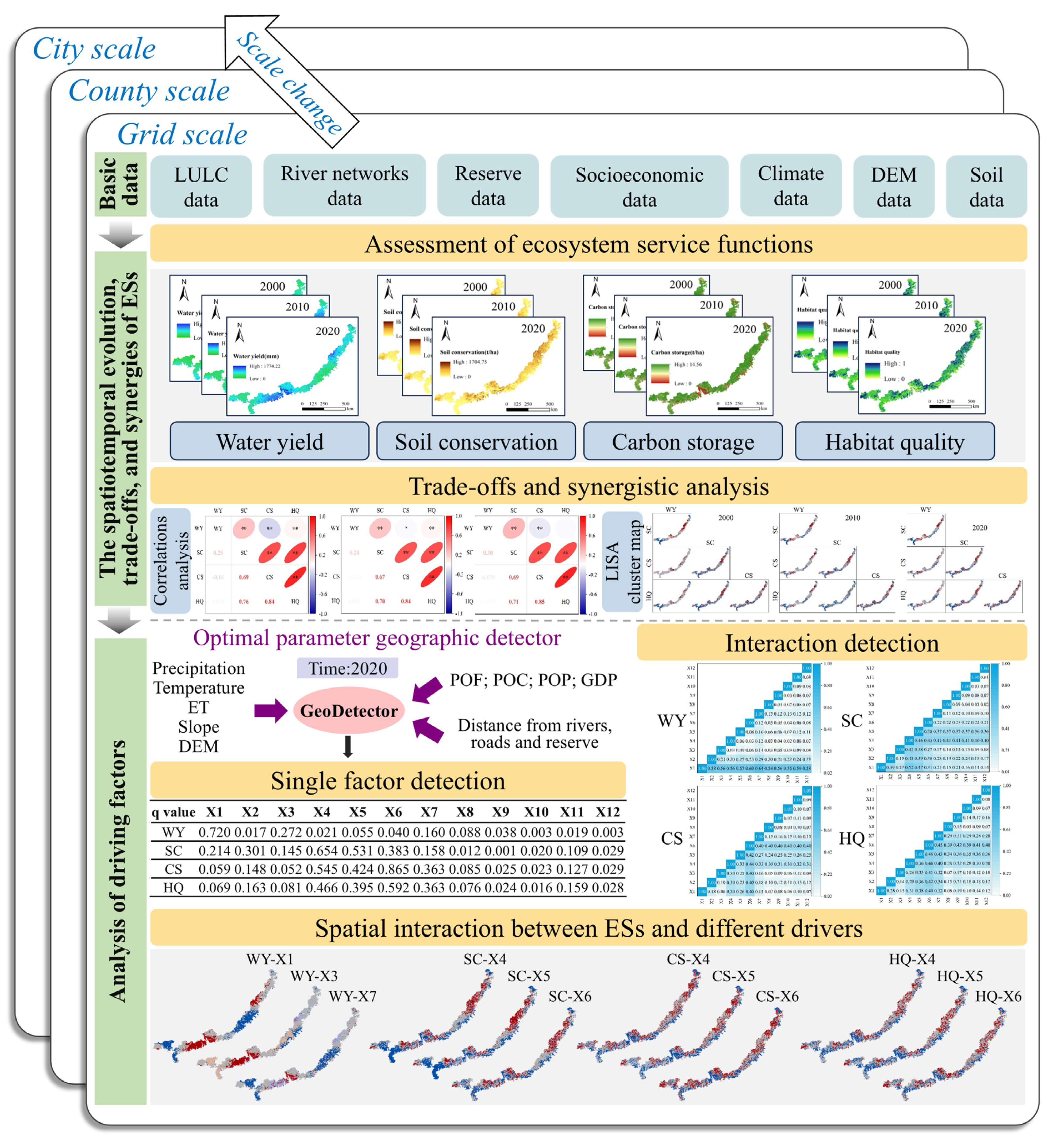
This study analyzes four ecosystem service functions from a multiscale perspective and clarifies the intensity and spatially aggregation attributes for ES trade-offs and synergies. By applying the Geodetector model, it scientifically diagnoses and identifies the dominant driving factors, quantifies their contributions. Thereby ultimately revealing the spatial heterogeneity of the dominant driving mechanisms across different scales through integration with the bivariate Moran’s I. Figure 2 illustrates the technical roadmap.

3. Results

3.1. Spatiotemporal Distribution Patterns of ESs

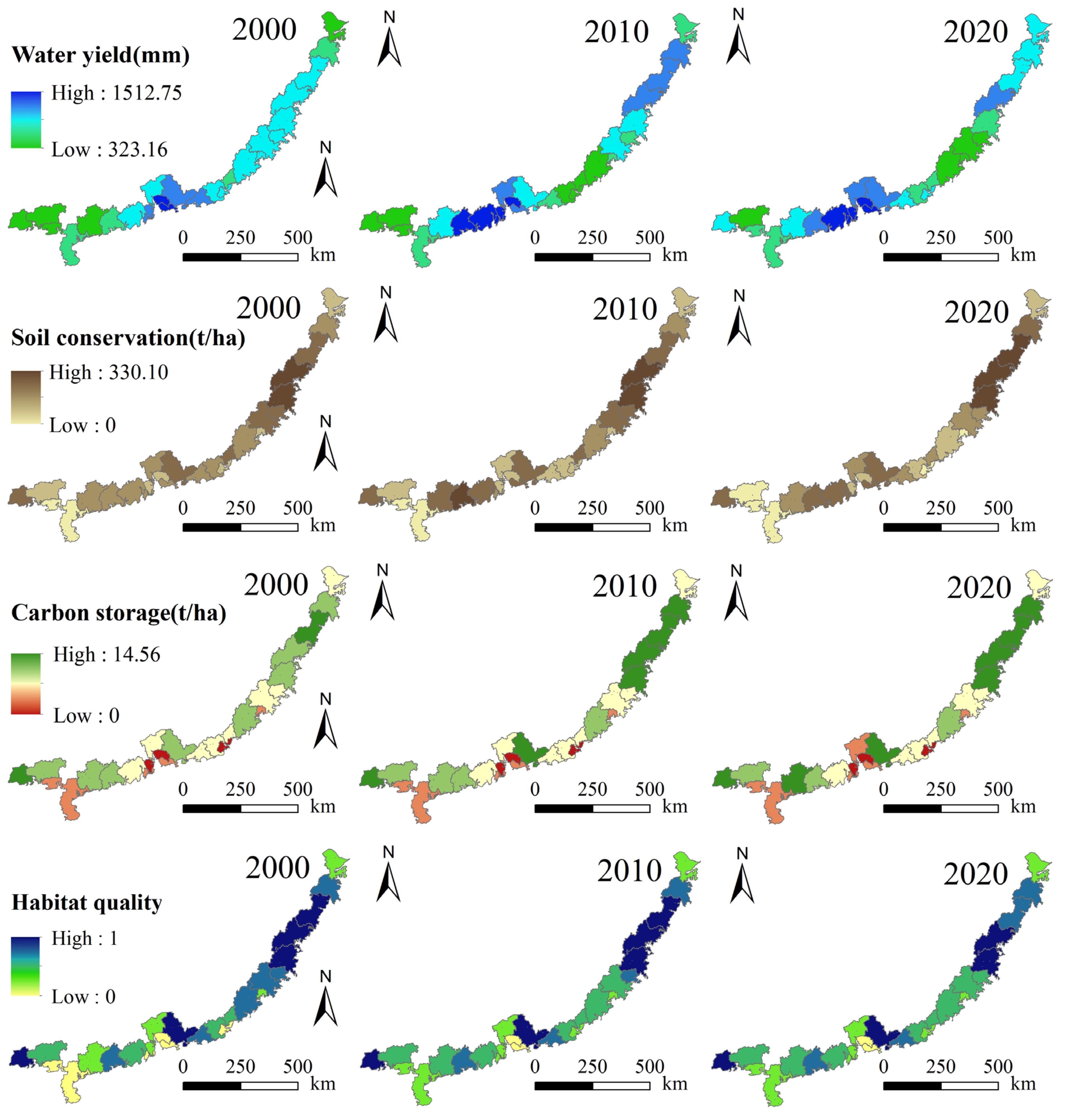
The four ESs in Southeast Coastal China exhibited distinct pattern contrasts across spatial scales from 2000 to 2020, with their spatial distributions showing increased clustering as the scale expanded. Each scale highlighted unique aspects of the spatiotemporal patterns.
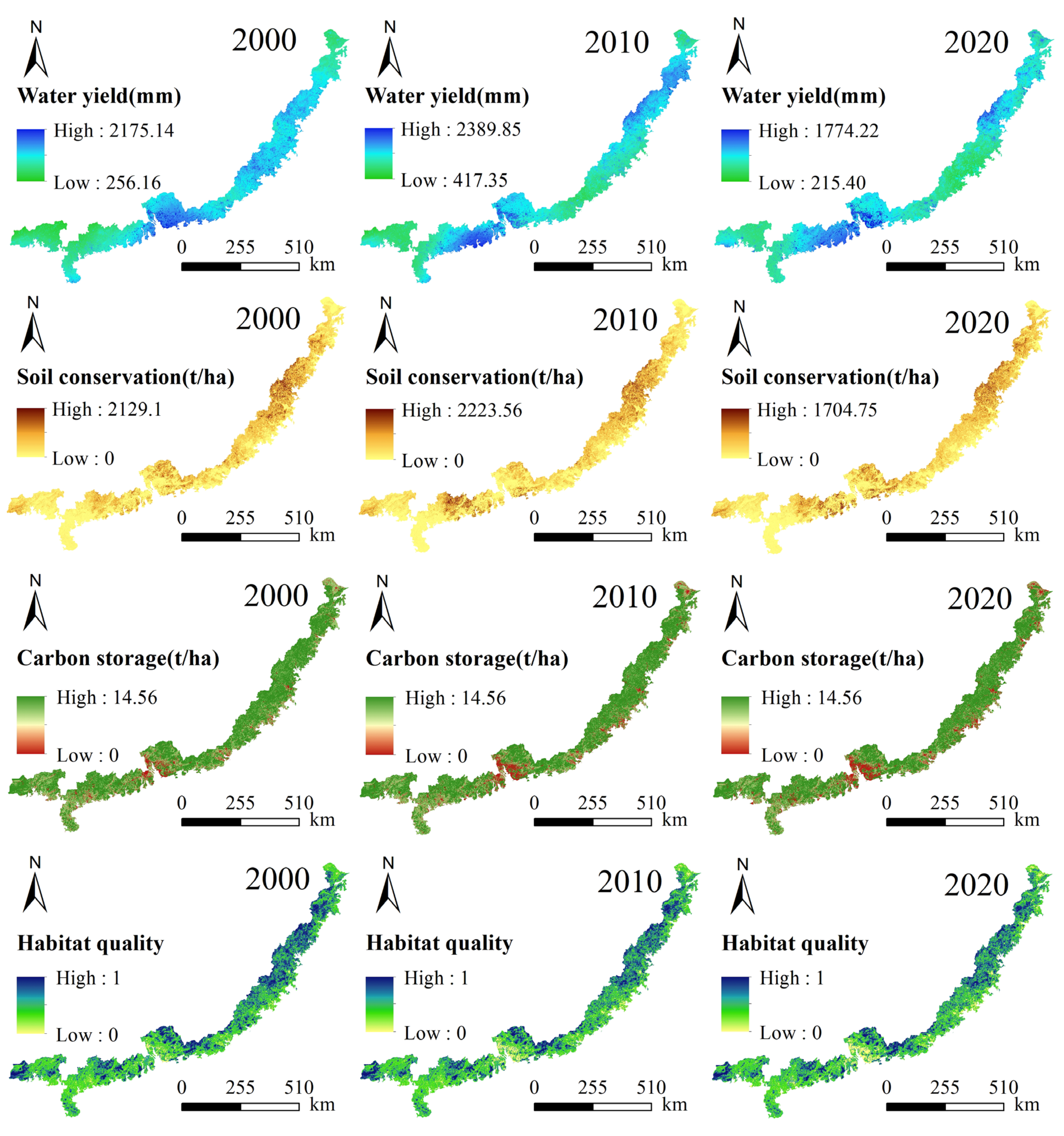
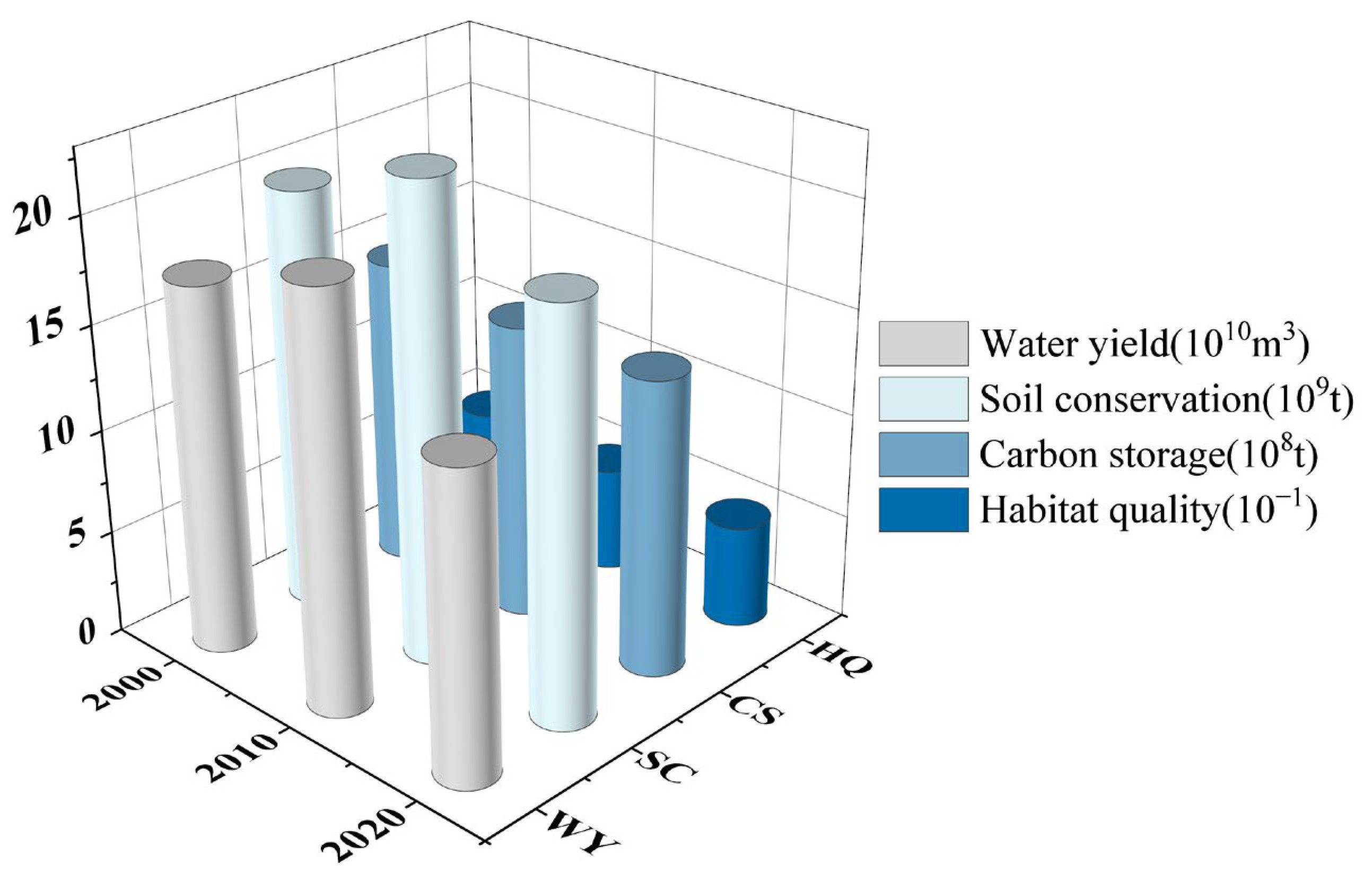
The grid scale (1 km) most clearly revealed the local details and spatial heterogeneity of ESs (Figure 3). High WY values mainly occurred in the Pearl River Delta and northeastern sections of the study area, where widespread impervious urban surfaces enhanced the rapid conversion of rainfall into runoff. Spatial expansion of low-WY zones was apparent, particularly in central agricultural domains where cultivated-dominated areas exhibited diminished WY. In the 2000–2020 ecosystem services statistics (Figure 4), WY followed a nonlinear trend, initially increasing before declining from 17.58 × 10¹⁰ m3 in 2000 to 14.63 × 10¹⁰ m3 in 2020. High SC areas were precisely located in forested hilly terrains of Guangdong and Guangxi, with low-value zones closely aligned with steep-sloped barelands and cultivated areas. Across the three periods, the SC also exhibited a trend of increasing initially followed by a decrease, with values of 20.2 × 10⁹ t, 22.6 × 10⁹ t, and 19.5 × 10⁹ t, respectively. The CS experienced persistent degradation, diminishing from 14.84 × 10⁸ t to 14.13 × 10⁸ t over the study period. Minimum CS values consistently occurred in low-forest-coverage environments, such as coastal valley regions. The average HQ values for 2000 to 2020 were 0.53, 0.50, and 0.49, indicating an overall declining trend. The HQ across the study area remained relatively low, particularly in the Pearl River Delta and the southern coast of Hangzhou Bay, where the decline became more pronounced alongside economic growth and accelerated urbanization.
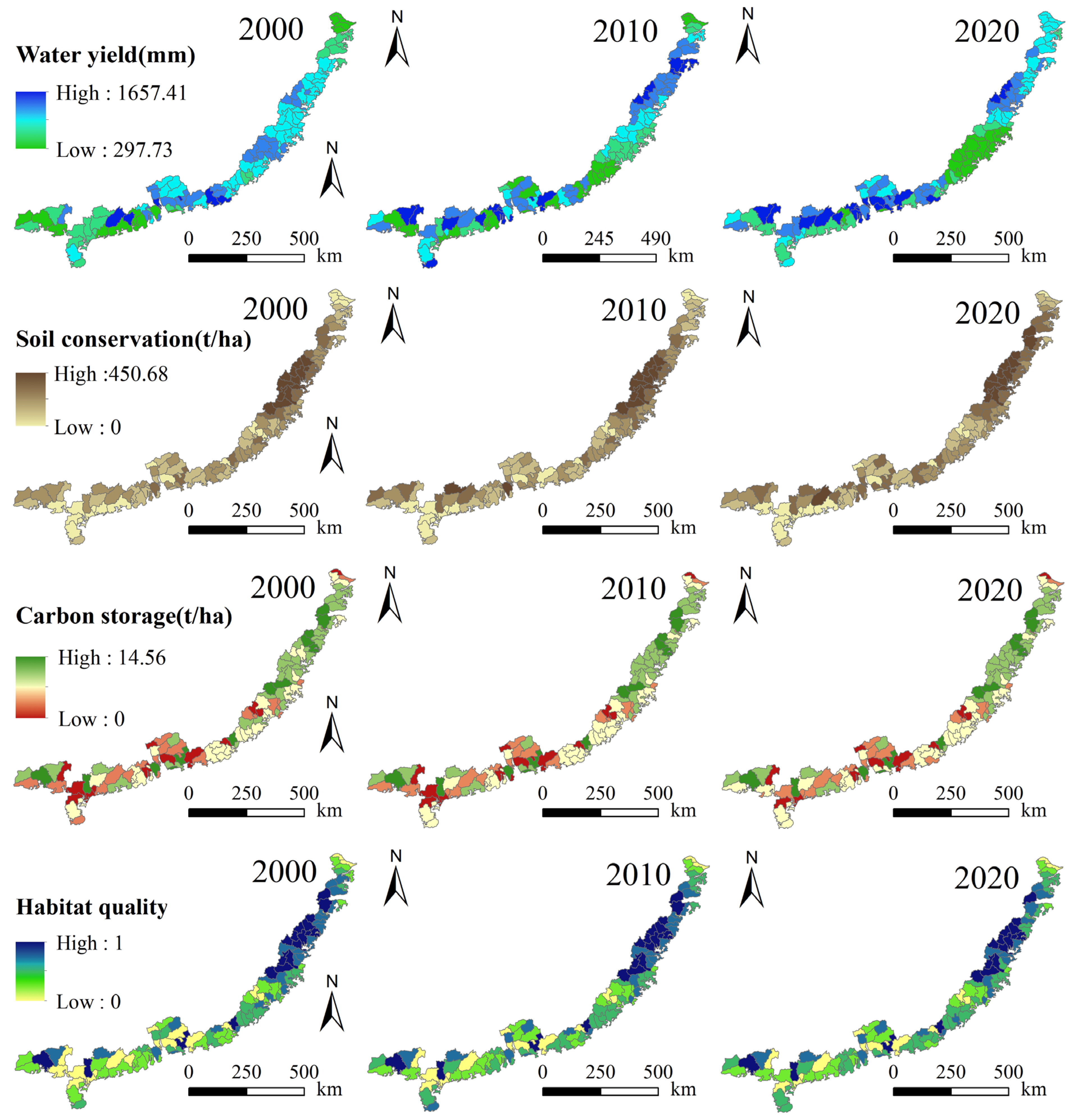
Compared to grid scale, the county scale amplified regional spatial divergence and polarization trends (Figure 5). At this scale, high and low-value clusters of ESs showed sharper boundaries. For instance, high WY values formed contiguous concentrations in southern Pearl River Delta counties and partial northeastern sectors. The SC maintained analogous spatial distributions across scales. The CS demonstrated insignificant variation over time, with high-value zones principally distributed within the Pearl River Delta. The high-value clustering areas of HQ are mainly preserved in northeastern territories, though their spatial extent displayed contraction at county-level resolutions.
The city scale captured macro-regional contrasts and the homogenization effect within administrative units (Figure 6). The WY displayed pronounced interannual fluctuations, particularly in the Pearl River Delta prefectures experiencing abrupt 2010 volume surges followed by 2020 declines. SC and HQ exhibited distribution characteristics consistent with those observed at the grid scale. The CS exhibited significant changes in the construction core area of the Pearl River Delta and the northeastern region. Under urbanization pressures, CS decreased in the Pearl River Delta’s construction core. CS increased in the northeastern part of the study area, such as Taizhou, Ningde, and Fuzhou. Inter-city variations in ESs were particularly notable, reflecting the dominant influence of macro-policies and regional development disparities.
Collectively, county-level analyses demonstrated enhanced polarization of ESs extremes compared to other scales. City assessments delineated environmental deterioration in Pearl River Delta conurbations contrasting with relative ecological preservation in northeastern administrative units.

3.2. Trade-Offs and Synergistic Relationships in ESs

3.2.1. Spearman’s Correlation Coefficients Among ESs

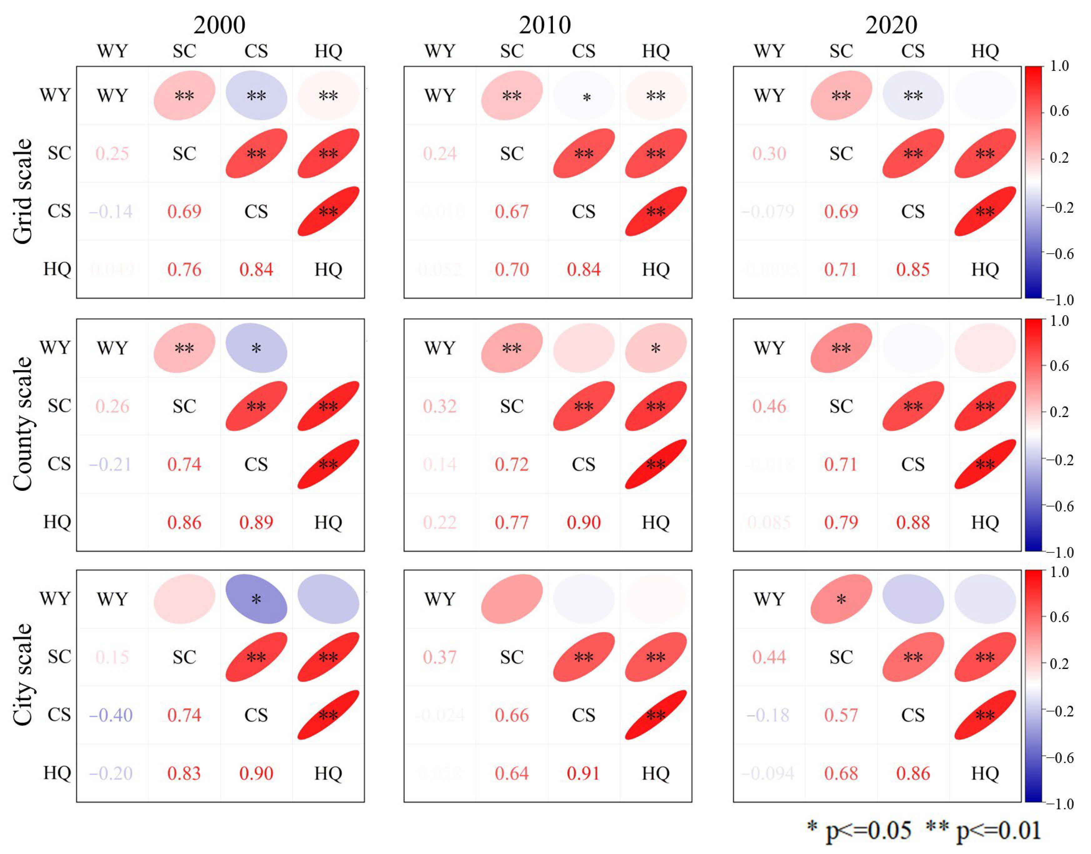
To explore spatial patterns of trade-offs and synergies among ESs, a bivariate autocorrelation analysis was applied across multiple scales in China’s southeastern coastal region, elucidating their spatiotemporal distribution characteristics. Six pairwise correlations among four ESs were identified, most of which exhibited significant correlations (p < 0.05) (Figure 7). Synergistic relationships persistently maintained between SC-CS, SC-HQ, CS-HQ, and WY-SC across all scales, suggesting potential functional complementarities in ecological processes and resource utilization.
At the grid scale, Spearman correlations between ES pairs showed that WY-HQ was only non-significant in 2020. WY-CS exhibited consistent negative correlations throughout the study period, while WY-HQ transitioned from positive (2000 and 2010) to negative (2020) correlations. CS-HQ demonstrated the strongest positive correlations across all temporal phases, with coefficients of 0.84, 0.84, and 0.85. Between 2000–2020, three ES pairs (WY-SC, WY-CS, CS-HQ) showed enhanced synergies or weakened trade-offs, whereas two pairs (WY-HQ, SC-HQ) experienced relationship degradation.
In the county-level analysis, significance patterns varied over time: five significant pairs were observed in 2000 and 2010 (excluding WY-HQ in 2000 and WY-CS in 2010), which declined to four in 2020 (excluding WY-SC and WY-HQ). Compared with grid-level assessments, absolute correlation coefficients were stronger, maintaining four to five positive correlations annually. CS-HQ consistently displayed the strongest positive correlations (0.88–0.90). Two ES pairs showed temporary improvement between 2000 and 2020, with WY-SC exhibiting the greatest increase in correlation, rising from 0.26 to 0.46.
At the city level, distinct inter-scale dynamics were observed, with four, three, and four significant pairs identified in respective years. Despite progressive degradation, CS-HQ consistently maintained the highest positive correlations, while SC-HQ sustained the second highest correlations (>0.6). Over time, three pairs (WY-SC, WY-CS, WY-HQ) showed improvement. The findings highlight scale-dependent interaction mechanisms, with county-level analyses demonstrating heightened ESs extremes differentiation, and city-level assessments revealing heterogeneous environmental trajectories between Pearl River Delta conurbations and northeastern regions.

3.2.2. Multiscale Spatial Agglomeration Characteristics of ESs

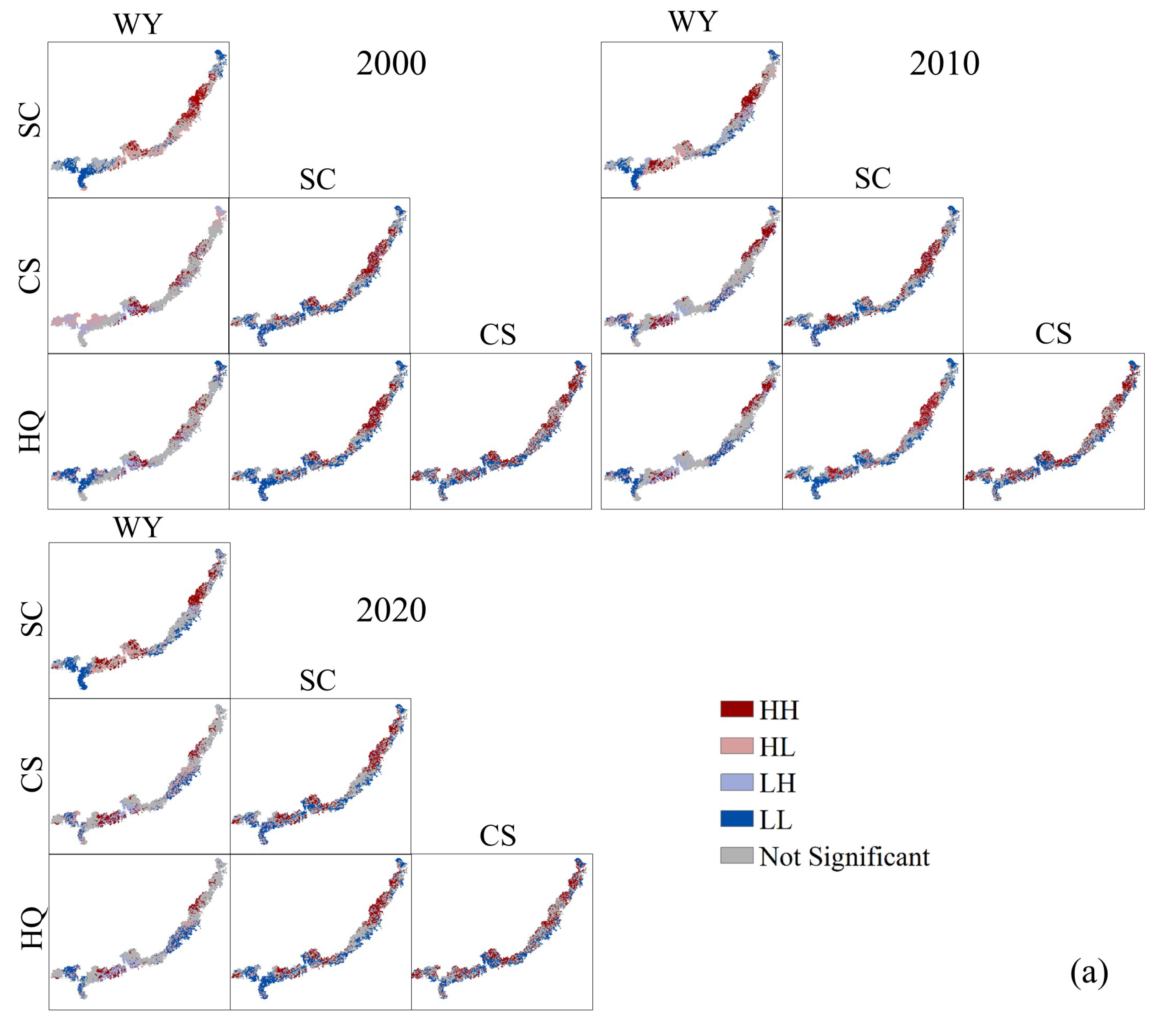
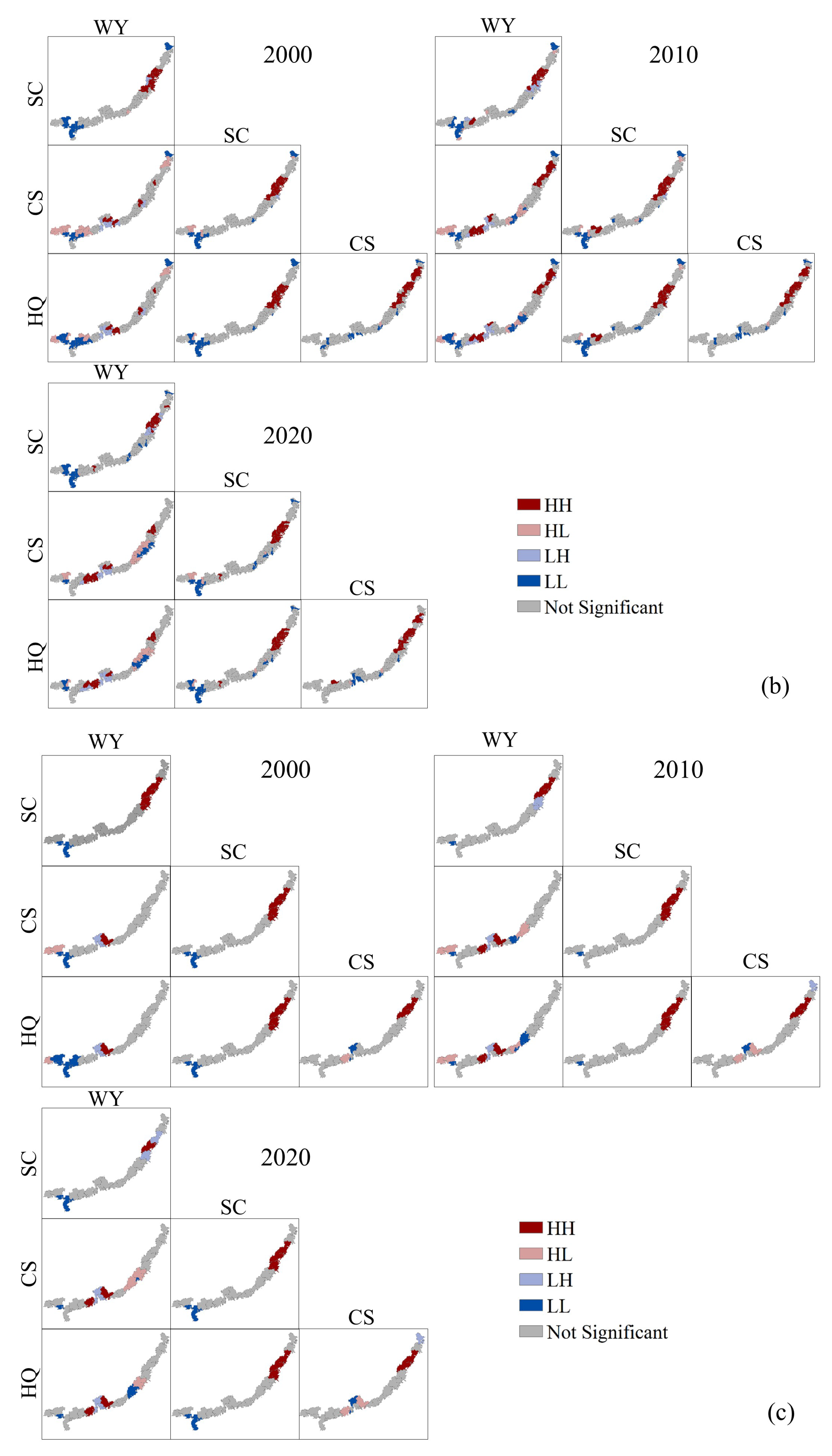
As illustrated in Figure 8, notable spatial variations exist in the trade-offs and synergies among ecosystem services, with interactions intensifying as the scale increases. For most ecosystem service pairs, the proportion of spatial synergy exceeds that of trade-offs, indicating that they are predominantly characterized by synergistic relationships. At both the grid and county scales, ESs in the northeastern part of the study area, where forests and grasslands are concentrated, exhibit HH synergistic relationships. At the grid scale, WY-SC in the Pearl River Delta shows an HL trade-off relationship, while other ecosystem service pairs in this region mostly display LL synergistic relationships. At the county scale, from 2000 to 2010, WY-CS in the southwestern part of the study area exhibits an HL trade-off relationship, suggesting potential competitive between ecological functions and resource utilization in this region. In the southern part of the study area, specifically the Leizhou Peninsula, most ES pairs show LL synergistic relationships. At the city level, the relationships among the six pairs of ESs exhibit fluctuating changes. SC maintains a dominant positive synergy with CS and HQ, while WY and CS are primarily characterized by trade-offs, with the trade-off area expanding annually. The relationship between WY and SC is dominated by positive synergy, although the synergistic area is gradually decreasing.

3.3. Driving Factors Analysis of ESs

3.3.1. Impact of Individual Factors on ESs

The GeoDetector was employed to identify key drivers influencing the spatial heterogeneity of ESs across multiple scales (Table 5), using 2020 as a case study. In this study, the corresponding significance levels (p-values) of all influencing factors were less than 0.01. For WY, X1 was the most critical driving factor (q = 0.720) at the grid scale, followed by X3 (q = 0.272). Both factors (X1 and X3) were crucial for the formation and variation in water distribution, and their q-values increased with the scale. Notably, the significant influence of X12 is only detected at the county scale (q = 0.213), indicating that X12 affects WY exclusively at this scale. For SC, the top three factors at the grid scale were X4 (q = 0.654), X5 (q = 0.531), and X6 (q = 0.383). X4 is associated with increased soil erosion, while X6 functions by enhancing vegetation cover and soil conservation capacity. The q-values of X4 and X6 also increase with the scale. By contrast, X5 reaches 0.909 at the county scale, far exceeding other scales, demonstrating that X5 is the dominant driver at the county scale. For CS, X6 has the highest q-value, followed by X4 and X5. As topographic factors, X4 and X5 directly or indirectly influence the spatial distribution of meteorological factors and soil texture. Additionally, different soil types also determine vegetation productivity and biological community composition to some extent within the study area. The q-values increase correspondingly with the scale. For HQ, X4, X5, and X6 are the top three factors with the highest q-values, among which X6 has the greatest impact on HQ, with q-values of 0.592, 0.778, and 0.841 across the three scales.
In summary, natural drivers exert a more significant impact on ESs than social drivers across the three scales. Among the natural factors, X4 and X5 are the most important driving factors. The impacts of different drivers on ESs exhibit marked variation across spatial scales, with the strength of drivers increasing as the scale expands.

3.3.2. Effects of Multifactor Interactions on ESs

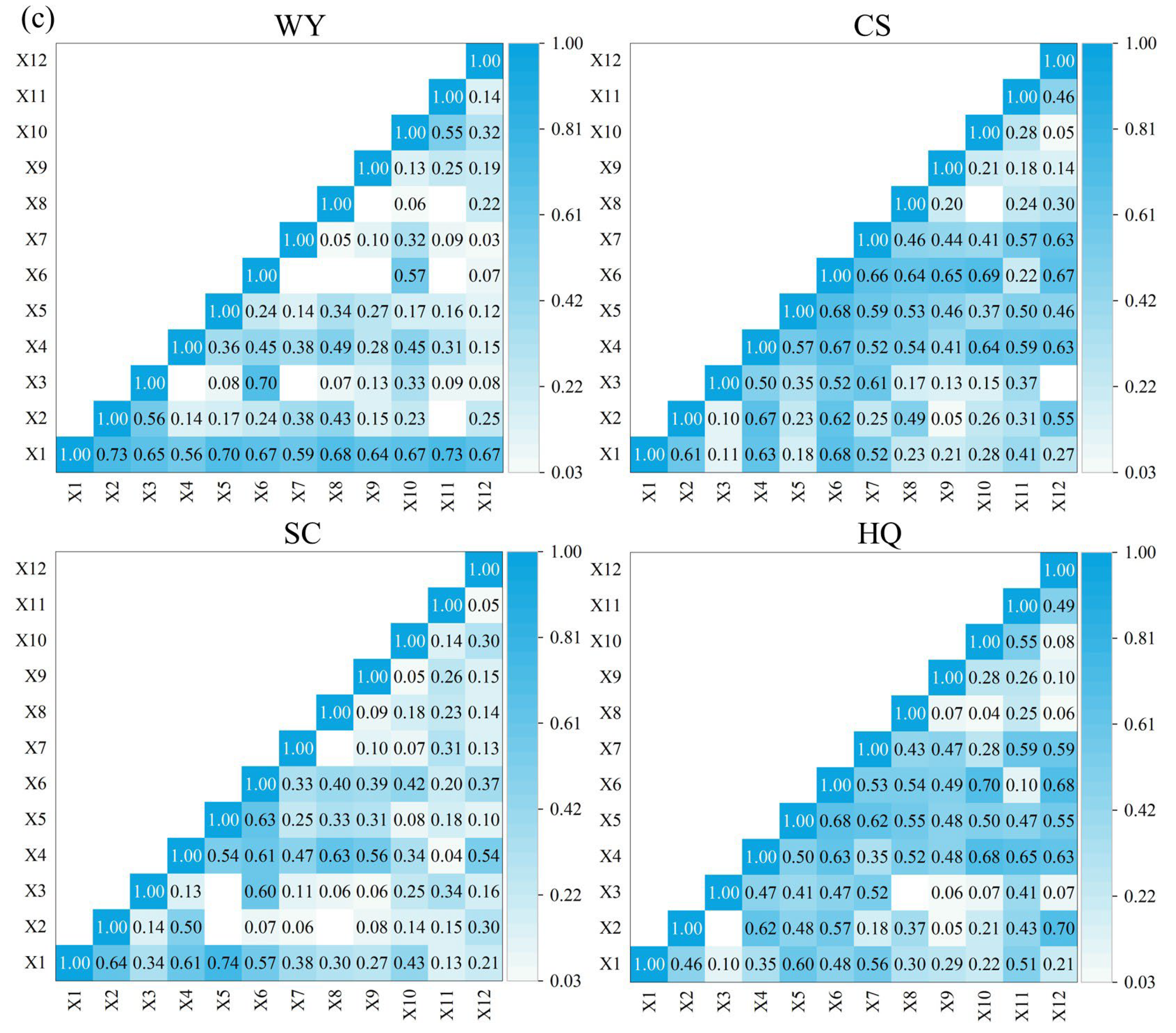
Figure 9 illustrates that the explanatory capacity of interacting factors is substantially greater than that of single variables. For WY, the interaction between X1 and other variables has the strongest effects, with the interaction between X1 and X7 yielding q values of 0.64, 0.65, and 0.59 across the three scales. In contrast, the interaction explanatory power between X3 and X6 is less than 0.1 at the grid and county scales, but reaches 0.70 at the city level. For SC, the interactions between X4, X5, and X6 and other drivers exhibit the highest explanatory capacity, especially between X1 and X4, with q-values of 0.52, 0.72, and 0.61 across the three scales. For CS, the interaction involving X6 consistently demonstrates the highest explanatory power across all scales. For HQ, with the exception of the interaction explanatory power between X2 and X7 at the city level being 0.18, the interactions between X4, X5, X6, and X7 and other factors have the highest q-values at the three scales.

3.4. Spatial Interaction Between ESs and Different Drivers

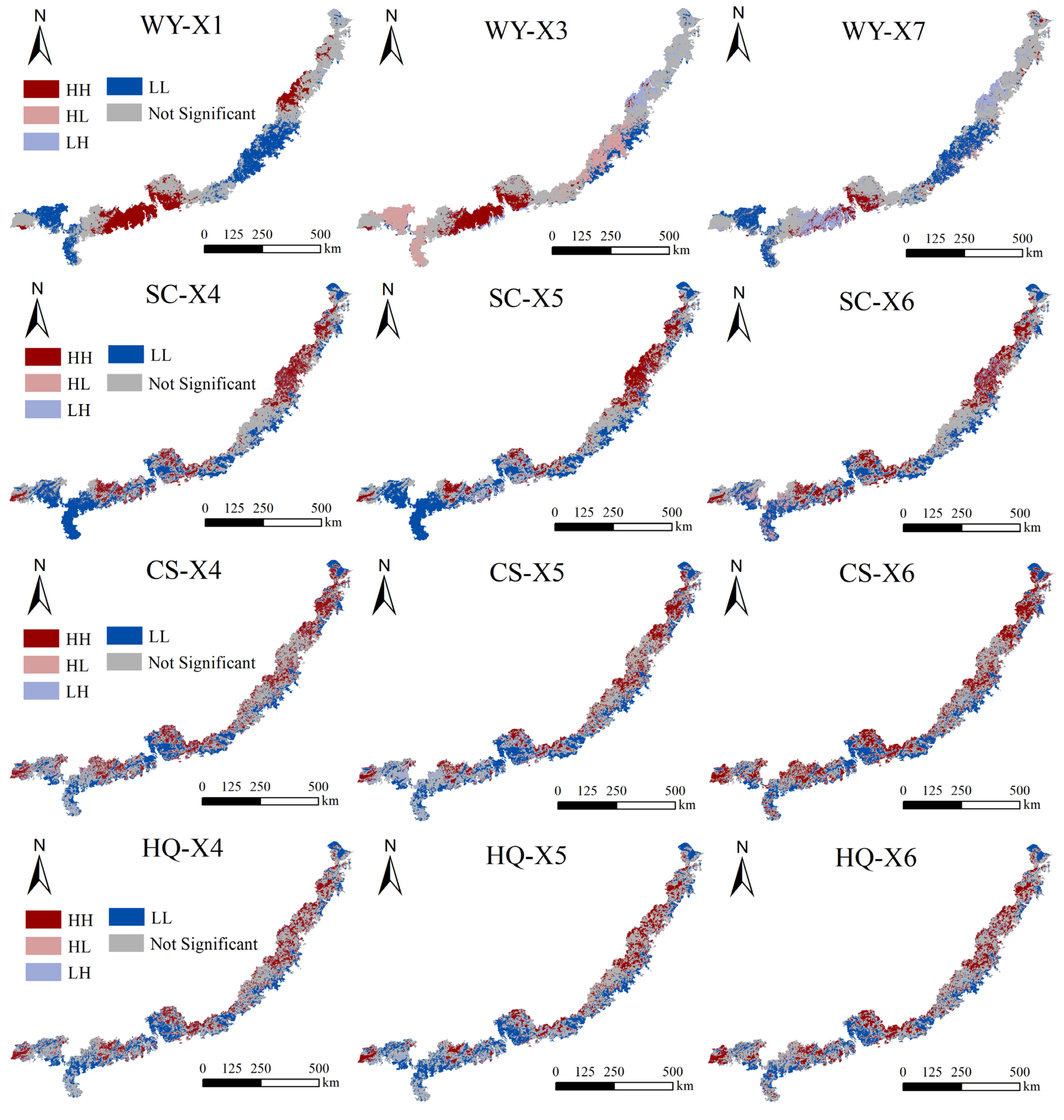
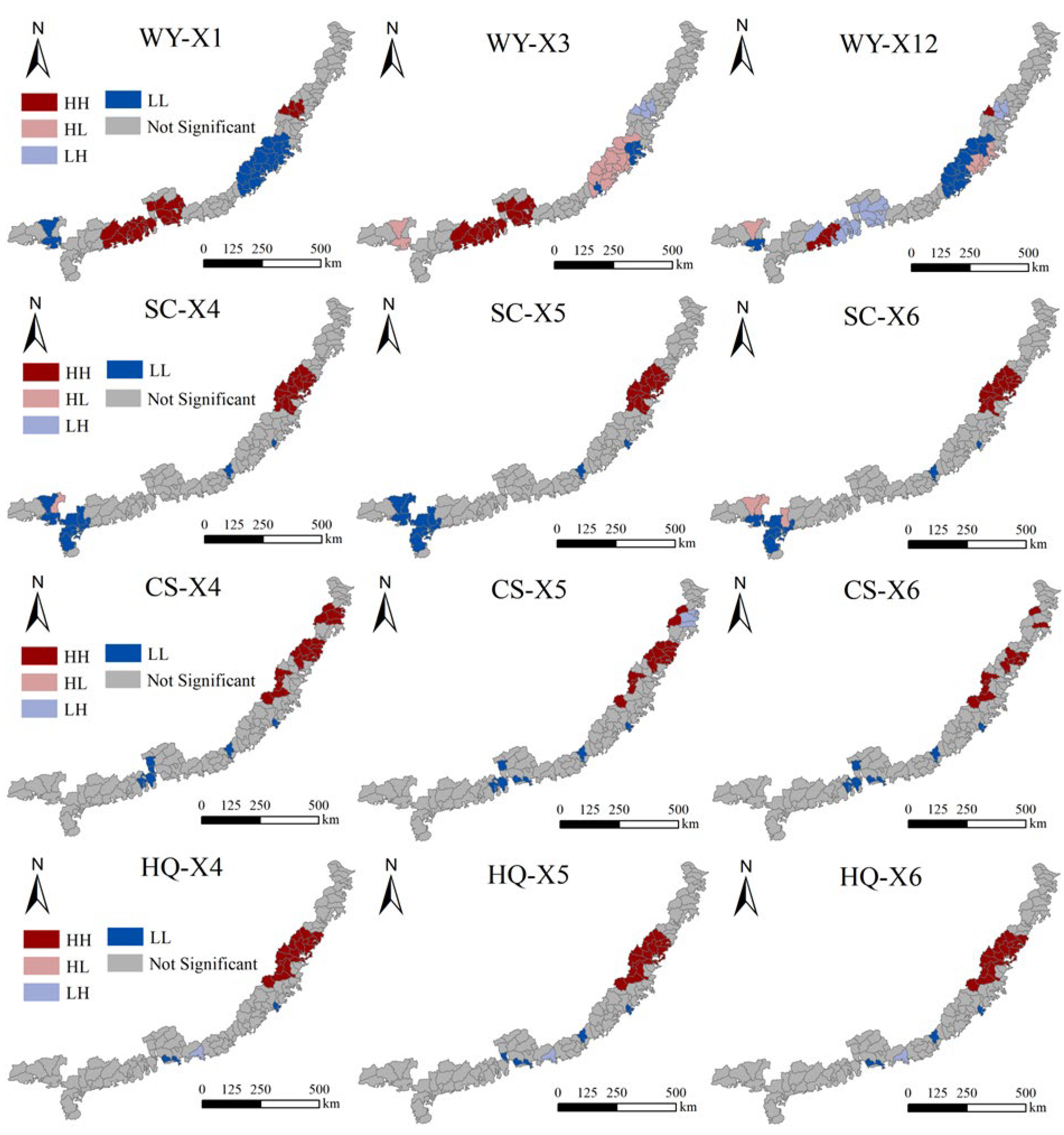
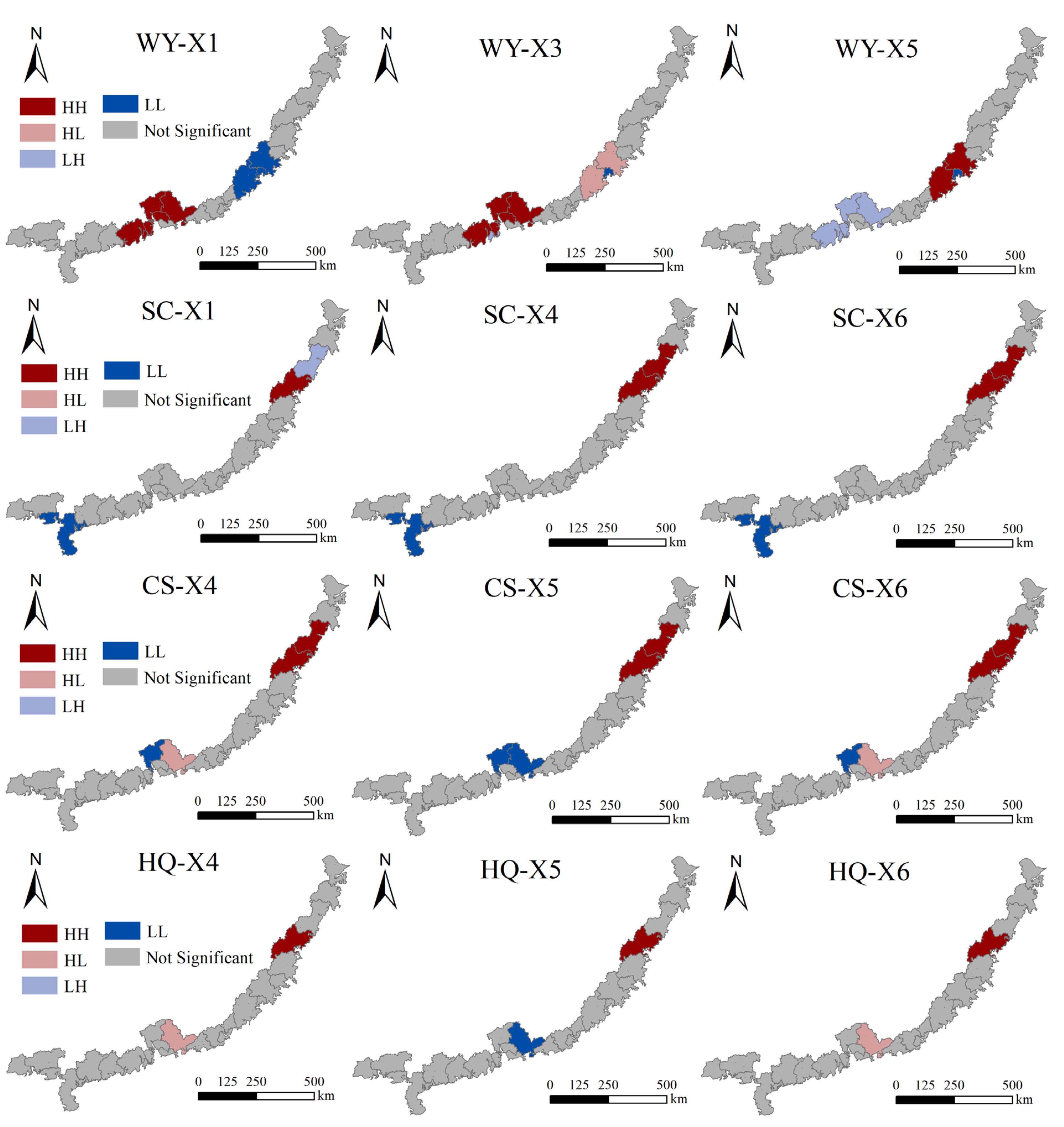
To demonstrate the spatial patterns of multiple factors influencing ESs, this study employed bivariate local Moran’s I to visualize the effects of key factors identified by the GeoDetector, and the interactions were presented through LISA maps [58]. LISA maps reveal the spatial interactions between ESs and drivers. The results are categorized into five types: HH, LL, HL, LH, and non-significant. For each spatial scale, the three drivers exhibiting the highest q-values, reflecting their relative influence on ecosystem services, were chosen for detailed spatial examination. The LISA spatial clustering results are shown in Figure 10, Figure 11 and Figure 12.
In the Pearl River Delta region in the southern part of the study area, WY-X1 exhibited significant scale stability, with both exhibiting HH clustering patterns across all three spatial scales. This aggregation characteristic indicates a significant positive correlation between X1 and WY, suggesting that an increase in X1 has a clear positive promoting effect on the enhancement of WY. Similarly, the HH clustering areas of WY-X3 were consistently distributed in the southern Pearl River Delta across all research scales, while the LL clustering areas were concentrated in the eastern coastal zone. Moreover, as the analysis scale expanded, the clustering type in this region gradually transitioned from LL to HL. At the grid scale, X7 had a significant influence on WY, with HH clustering areas distributed near the southern Pearl River Delta regions and LL clustering areas in the eastern coastal region. For SC, the influencing areas of SC-X4, SC-X5, and SC-X6 highly overlapped at both the grid and county scales, indicating a comprehensive driving effects of these factors on SC. Specifically, HH clustering areas for these factors were consistently located in the eastern part of the study area at both scales, while LL clustering areas were concentrated near Leizhou City in the southwestern part of the study area. When the scale was elevated to the city level, the dominant factors influencing soil retention shifted, with X1, X4, and X6 becoming the primary factors. Regarding the driving mechanisms of CS and HQ, the three research scales exhibited a high degree of consistency: X4, X5, and X6 consistently served as the core influencing factors for both. Their HH clustering areas were sporadically distributed in the northeastern part of the study area at all scales. At the grid scale, LL clustering areas were distributed along the southern coast, while at the county scale, the clustering was less pronounced.

4. Discussion

4.1. Spatiotemporal Interactions of LULC Changes with Changes in ESs

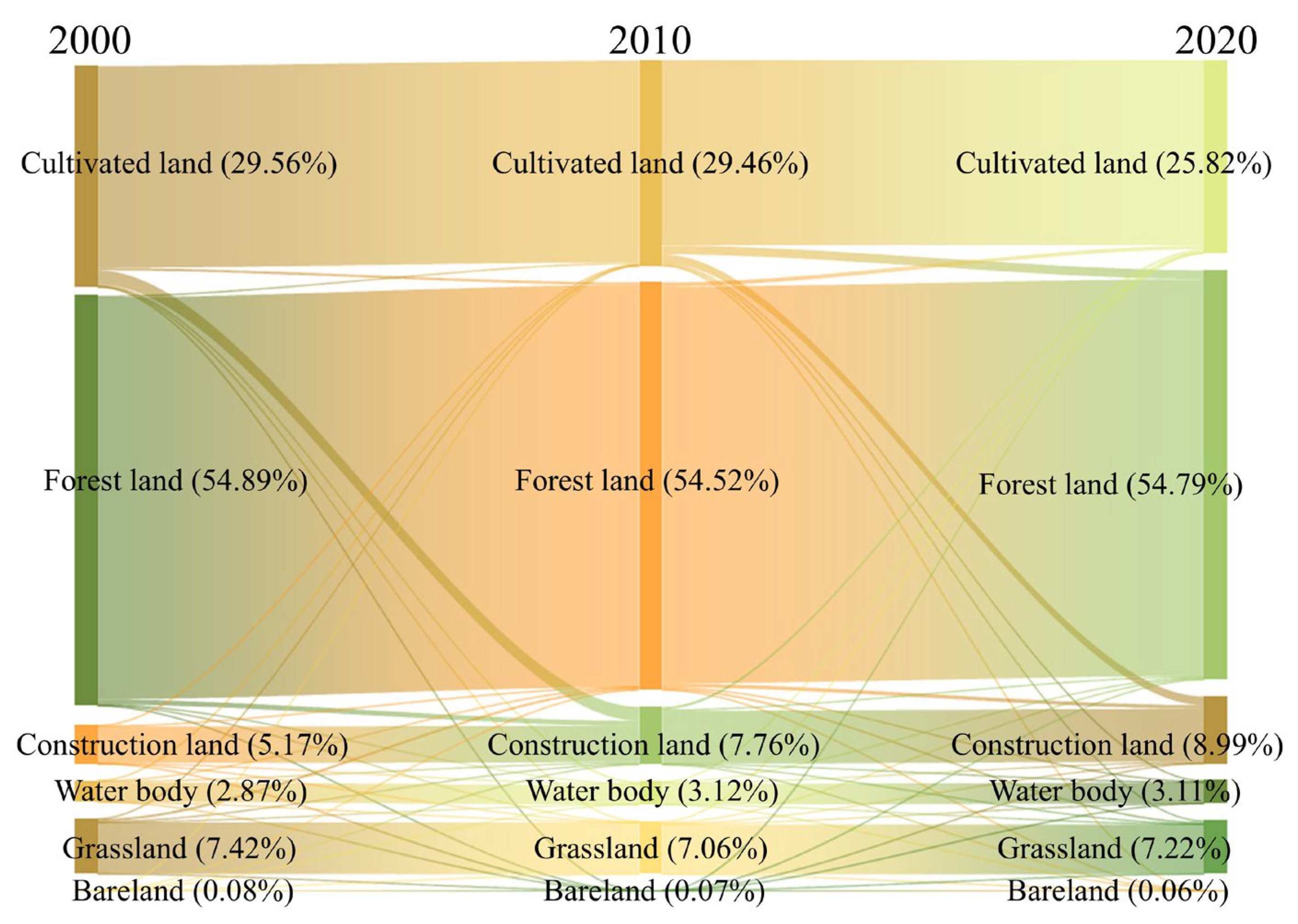
This paper examines the dynamics of LULC changes, emphasizing the interchanges among cultivated land, forests, and construction areas. These three categories together represent 89% of the total area that experienced conversion. As illustrated in Figure 13, forests are the most prevalent LULC type, accounting for 50% of the total land use. Cultivated land is primarily distributed in flat, strip-like areas, constituting 29% of the total LULC types. Most rivers and canals form narrow strips running roughly east–west, ultimately converging with the sea to the east. From 2000 to 2020, construction land expanded, while cultivated and forest land decreased (Figure 14). Specifically, 2.92% of cultivated land and 1.06% of forest land were converted into construction land (Table 6). Land changes are particularly significant along the southern shore of Hangzhou Bay and the Pearl River Delta region, where the flat topography, developed economy, and dense population provide favorable conditions for the expansion of construction land. Along the southern coastline, LULC remained relatively stable due to the influence of mountainous and bedrock coasts. With the acceleration of urbanization, regions close to central cities experienced a more rapid decline in ES values. Once economic development attains a certain level, harmonious coexistence of economic growth and ecological sustainability should be achieved [59].
Between 2000 and 2020, most land transformed into water bodies originated from cultivated land, covering an area of 766.9 km2. Furthermore, from 2010 to 2020, certain portions of cultivated land were transformed into forest through ecological restoration initiatives such as returning farmland to forests and grasslands. During this period, CS and HQ decreased less due to the slow rebound of forest areas and increased state control of poldering. Total WY was largest in forested areas. From 2000 to 2010, the decline in ESs was due to coastal construction land expansion, a reclamation, and the encroachment on forest and grassland [60]. Between 2010 and 2020, efforts to convert farmland into forest and grassland resulted in a gradual increase in forested areas and a notable reduction in cultivated land. This transformation contributed to a recovery in the annual average value of ESs in the study region. To continuously enhance ecosystem services, it is recommended to implement spatially differentiated land use control strategies. In areas experiencing the most intensive expansion of construction land, such as the Pearl River Delta, strict urban growth boundaries should be established, and compact urban development models should be promoted to curb further encroachment on cultivated land and forest areas [61]. Simultaneously, conservation efforts should focus on preserving existing forest patches and water bodies. In the northeastern hilly regions where forest ecosystems remain relatively intact, the demarcation of ecological conservation redlines should be strengthened to maintain the continuity of forest vegetation. Additionally, the protection of major river ecological corridors should be systematically enhanced to ensure landscape connectivity.

4.2. Scale Effects of Ecosystem Services and Ecosystem Services Trade-Offs and Synergies

The study reveals that the interactions among ESs exhibit significant scale dependency [62,63], with the county scale demonstrating the strongest correlations (as shown in Figure 7). At the grid scale, local heterogeneity dominates ES relationships, failing to capture broader functional linkages. When the scale is expanded to the city scale, the units encompass highly heterogeneous landscapes, and the spatial aggregation process oversimplifies the complex nonlinear relationships within [64,65]. In contrast, the county scale achieves an optimal balance in capturing medium-sized landscape patterns shaped by the interaction of topography and human activities, thereby most clearly revealing the intrinsic functional connections among ESs and allowing synergistic processes such as soil conservation, carbon storage, and habitat quality to be fully expressed.
Notably, we observed the interesting phenomenon that the relationship between WY and HQ reversed from synergy to trade-off at the city scale (Figure 7). with its underlying mechanism stemming from the fundamental reshaping of ecological processes by human activities at the city scale [66]. At finer scales (grid and county levels), the synergistic relationship between WY and HQ is primarily governed by the regulatory function of natural vegetation. Dense vegetation cover regulates runoff through canopy interception and enhanced soil infiltration, while simultaneously providing high-quality habitats. However, at the city scale, large-scale and centralized human activities (such as rapid urbanization and industrial zoning) become the dominant force, fundamentally altering hydrological processes and intensifying habitat fragmentation. Firstly, regarding the impact on WY: large-scale urban development leads to the extensive replacement of natural surfaces with impervious layers (e.g., asphalt, concrete). These impervious surfaces drastically reduce rainfall infiltration, converting originally slow subsurface flow into rapidly accumulating surface runoff. Consequently, this significantly increases the total water yield at the macro level, but at the cost of diminished water conservation capacity and disruption of the hydrological cycle. Secondly, regarding the impact on HQ: the urbanization process fragments continuous natural landscapes into isolated habitat patches. The expansion of industrial zones, transportation networks, and built-up areas directly encroaches upon and destroys plant and animal habitats, resulting in a sharp decline in HQ at the regional level.
Therefore, the trade-off relationship between WY and HQ observed at the city scale essentially represents the inherent contradiction between “high water yield driven by human activities” and “high habitat quality maintained by natural ecosystems.” The spatial aggregation effect accentuates this regional polarization based on distinct land use types: highly urbanized administrative units (such as Shenzhen and Guangzhou) contribute to high WY but low HQ, while ecological conservation areas exhibit the opposite characteristics. This reversal in relationship signifies a shift in the dominant processes from local natural ecological regulation to regional socioeconomic drivers.
In contrast, the synergistic relationships among SC, CS, and HQ remain stable across scales because they collectively and directly depend on relatively stable natural capital like vegetation and topography, exhibiting more consistent response patterns to human-induced land use changes [48,65].

4.3. Spatial Heterogeneity Attribution of Driving Factors for ESs

The scale evolution of single-factor driving forces indicates that the dominant forces shaping ecological patterns shift with the observational scale. At the grid scale, natural factors (e.g., X4, X5, X6) exhibit the strongest explanatory power for ESs (especially SC, CS, and HQ). The spatial autocorrelation analysis results (Figure 10) show that their HH synergy clusters are stably distributed in the forested hilly areas of the northeastern study area. This spatial pattern confirms that topography and forest coverage jointly constitute a stable natural baseline that maintains high levels of carbon storage and biodiversity in this region. It also verifies that ecological processes at the micro-unit level are primarily constrained by the physical conditions of topography and vegetation [67,68,69]. However, as the scale expands to the city level, the q-values of natural factors increase relatively gradually, while the explanatory power of human factors (e.g., X7, X8, X9) rises sharply. Observing Table 5, the explanatory power (q-value) of population (X8) on CS increases from 0.085 at the grid scale to 0.568 at the city scale. This finding reveals that within macro administrative units, the spatial aggregation effects of human activities (e.g., urbanization, industrial agglomeration) intensify, gradually becoming the dominant force shaping the broad patterns of ESs [70]. This underscores that the formulation of ecological management policies must be grounded in a clear scale perspective: at the local level, it is essential to protect key natural elements, while at the regional level, the focus should shift to regulating the intensity and patterns of human activity agglomeration [71].
An in-depth analysis of the interaction detector results reveals two distinct patterns of driving force enhancement governing the spatial heterogeneity of ESs, refining our understanding of multi-scale driving mechanisms. First, interactions between factors of the same type demonstrate a robust enhancement effect. Whether among natural factors or anthropogenic factors, the explanatory power of their interactions is generally greater than the individual contribution of any single factor. This pattern confirms the integrated nature of ecological processes, suggesting that drivers of the same type do not operate in isolation but collectively shape ES patterns through intrinsic synergistic or trade-off mechanisms. The more critical finding is the “lever effect” observed in natural–anthropogenic factor interactions. This manifests as a significant amplification of the influence of relatively weak anthropogenic factors when they couple with dominant natural factors. At the grid scale, the individual explanatory powers of construction land (X7), population (X8), and GDP (X9) for WY were only 0.160, 0.088, and 0.038, respectively, indicating limited independent influence. However, when interacting with mean annual precipitation (X1), their explanatory powers surged to 0.64, 0.54, and 0.56, representing a remarkable enhancement. Similarly, at the county scale, the single-factor explanatory power of construction land (X7) for CS was 0.555, which increased to 0.671 after interaction with forest coverage (X6) (X6∩X7). These findings mechanistically illuminate the critical moderating role of the natural baseline on the ecological effects of human activities. Empirical evidence demonstrates that human activities of identical intensity can yield markedly different ecological outcomes depending on the underlying natural conditions. This effect underscores that assessing and managing the impacts of human activities on ecosystems must fully account for their physiographic setting, as the natural baseline not only sets the ceiling of ecological potential but also modulates the ultimate ecological effects of anthropogenic interventions [72].

4.4. Limitations and Future Research

This study integrates multi-source data, various models and analytical methods to systematically investigate the spatiotemporal variations in ESs and their driving factors at multiple spatial scales in China’s southeastern coastal region. The findings have theoretical and practical significance, but there are still some limitations. With the acceleration of industrialization and the increase in pollutant emissions, human activities have an increasingly significant impact on ecosystem degradation. In this context, population, GDP, and LUCC were selected as key indicators to assess anthropogenic impacts, offering an initial understanding of the relationship between human activities and ecosystem dynamics. Nevertheless, these indicators do not fully capture the multidimensional aspects of human activities. Future research should expand the indicator system by incorporating additional variables that better reflect the intensity and modes of human disturbances to ecosystems, thereby enabling a more precise understanding of the underlying mechanisms. This study focused on analyzing four typical and critical types of ecosystem services, with some model input parameters referenced from corresponding parameters in related studies of similar regions. Although the current model accuracy met the requirements of this study, more locally accurate parameter data, such as carbon density, could be obtained through field measurements to enhance the accuracy of ES estimation in future research.

5. Conclusions

In this study, the spatiotemporal distribution of four ESs was estimated across three spatial scales during 2000–2020, and the trade-offs and synergies among different ESs were quantified. To reveal the underlying mechanisms, the impacts of driving factors on ESs were investigated from both individual effects and multifactorial interactions, clarifying the independent influence of single factors as well as the interactive effects resulting from multifactorial coupling. On this basis, spatial autocorrelation analysis was employed to uncover the spatial aggregation patterns between ESs and key drivers. The conclusions are as follows:
(1)
Among the four ESs assessed in this study, three (excluding water yield) exhibited a spatial pattern of increasing provision from coastal to inland areas. All four ESs demonstrated significant scale dependency in their spatial distributions, with clustering intensity notably strengthening as the analytical scale expanded from grid to city level.
(2)
Synergistic relationships dominated the interactions among ESs, with correlation strength generally intensifying at larger spatial scales. The strongest functional connections were consistently observed at the county scale.
(3)
Natural factors were identified as the dominant drivers of ES patterns, exhibiting greater influence than anthropogenic factors. The explanatory power of both driver categories increased with spatial scale. From an interaction perspective, interactions between factors of the same type generally yielded stronger explanatory power than any single factor. Furthermore, interactions between anthropogenic and natural factors significantly enhanced the explanatory power of individual anthropogenic factors.
(4)
The spatial aggregation patterns between ESs and their driving factors varied considerably across different drivers. However, for any given driver, its spatial association with a specific ES remained highly consistent across different spatial scales, demonstrating remarkable pattern stability.
The research suggests that evaluating the drivers affecting ecosystem services requires prioritizing appropriate spatial scales before introducing indicators encompassing natural, socio-economic, and human activities. Enhancing the synergistic benefits of ecosystem services and mitigating trade-offs are of significant importance for ensuring the steady growth of ecological health and the sustainable development in the southeastern coastal areas of China.

Supplementary Materials

The following supporting information can be downloaded at: https://www.mdpi.com/article/10.3390/land14112101/s1, Table S1. Parameter table of Water yield model. Table S2. Parameter table of soil conservation model. Table S3. The carbon density of each land use/land cover (Mg ha−1). Table S4. The sensitivity of habitat types to each threat factor. Table S5. Habitat suitability and sensitivity of habitat types to each threat factor.

Author Contributions

Conceptualization, H.Z., X.F. and J.H.; methodology, H.Z., X.F. and J.H.; software, H.Z., X.F. and J.H.; validation, H.Z., X.F. and J.H.; formal analysis, H.Z.; investigation, X.F. and Y.W.; resources, X.F. and Z.X.; data curation, Y.W.; writing—original draft preparation, H.Z., X.F. and J.H.; writing—review and editing, X.F. and Y.W.; visualization, H.Z. and J.H.; supervision, X.F. and Z.X.; project administration, X.F. and Y.W.; funding acquisition, X.F. All authors have read and agreed to the published version of the manuscript.

Funding

This research was funded by the National Key Research and Development Program of China, grant number 2022YFB3902200; National Natural Science Foundation of China, grant number 42571546.

Data Availability Statement

The data presented in this study are available in the article.

Conflicts of Interest

The authors declare no conflicts of interest.

References

  1. Cochran, F.; Daniel, J.; Jackson, L.; Neale, A. Earth observation-based ecosystem services indicators for national and subnational reporting of the sustainable development goals. Remote Sens. Environ. 2020, 244, 111796. [Google Scholar] [CrossRef]
  2. Wen, L.; Li, B.; Peng, Y.; Zhou, Y.; Weng, A.; Jin, Y.; Cai, G.; Lin, Y.; Chen, B. Exploring the evolution of coupled natural-cultural ecosystem services and their geographically scaled driven modeling in a coastal city of Southeast China. J. Environ. Manag. 2024, 361, 121265. [Google Scholar] [CrossRef]
  3. Morán-Ordóñez, A.; Ramsauer, J.; Coll, L.; Brotons, L.; Ameztegui, A. Ecosystem services provision by Mediterranean forests will be compromised above 2 °C warming. Glob. Chang. Biol 2021, 27, 4210–4222. [Google Scholar] [CrossRef] [PubMed]
  4. Fahad, S.; Sonmez, O.; Saud, S.; Wang, D.; Wu, C.; Adnan, M.; Turan, V. Sustainable Soil and Land Management and Climate Change; CRC Press: Boca Raton, FL, USA, 2021. [Google Scholar]
  5. Brauman, K.A.; Daily, G.C.; Duarte, T.K.e.; Mooney, H.A. The Nature and Value of Ecosystem Services: An Overview Highlighting Hydrologic Services. Annu. Rev. Environ. Resour. 2007, 32, 67–98. [Google Scholar] [CrossRef]
  6. Qiao, X.; Gu, Y.; Zou, C.; Xu, D.; Wang, L.; Ye, X.; Yang, Y.; Huang, X. Temporal variation and spatial scale dependency of the trade-offs and synergies among multiple ecosystem services in the Taihu Lake Basin of China. Sci. Total Environ. 2019, 651, 218–229. [Google Scholar] [CrossRef]
  7. Zhang, Y.; Wu, X.; Wang, S.; Zhou, Y.; Fu, F.; Lu, N.; Kou, L. Land use optimization for future ecosystem service demands: A case study in the Yanhe watershed. J. Clean. Prod. 2025, 520, 146121. [Google Scholar] [CrossRef]
  8. Xu, J.; Wang, S.; Xiao, Y.; Xie, G.; Wang, Y.; Zhang, C.; Li, P.; Lei, G. Mapping the spatiotemporal heterogeneity of ecosystem service relationships and bundles in Ningxia, China. J. Clean. Prod. 2021, 294, 126216. [Google Scholar] [CrossRef]
  9. Hou, Y.; Lü, Y.; Chen, W.; Fu, B. Temporal variation and spatial scale dependency of ecosystem service interactions: A case study on the central Loess Plateau of China. Landsc. Ecol. 2017, 32, 1201–1217. [Google Scholar] [CrossRef]
  10. Wang, Z.; Xu, M.; Lin, H.; Qureshi, S.; Cao, A.; Ma, Y. Understanding the dynamics and factors affecting cultural ecosystem services during urbanization through spatial pattern analysis and a mixed-methods approach. J. Clean. Prod. 2021, 279, 123422. [Google Scholar] [CrossRef]
  11. Bai, Y.; Chen, Y.; Alatalo, J.M.; Yang, Z.; Jiang, B. Scale effects on the relationships between land characteristics and ecosystem services- a case study in Taihu Lake Basin, China. Sci. Total Environ. 2020, 716, 137083. [Google Scholar] [CrossRef]
  12. Kusi, K.K.; Khattabi, A.; Mhammdi, N.; Lahssini, S. Prospective evaluation of the impact of land use change on ecosystem services in the Ourika watershed, Morocco. Land Use Policy 2020, 97, 104796. [Google Scholar] [CrossRef]
  13. Li, S.; Tu, B.; Zhang, Z.; Wang, L.; Zhang, Z.; Che, X.; Wang, Z. Exploring new methods for assessing landscape ecological risk in key basin. J. Clean. Prod. 2024, 461, 142633. [Google Scholar] [CrossRef]
  14. Zeng, S.; Jiang, C.; Bai, Y.; Wang, H.; Liu, E.; Guo, L.; Chen, S.; Zhang, J. Understanding scale effects and differentiation mechanisms of ecosystem services tradeoffs and synergies relationship: A case study of the Lishui River Basin, China. Ecol. Indic. 2024, 167, 112648. [Google Scholar] [CrossRef]
  15. Li, Y.; Luo, H. Trade-off/synergistic changes in ecosystem services and geographical detection of its driving factors in typical karst areas in southern China. Ecol. Indic. 2023, 154, 110811. [Google Scholar] [CrossRef]
  16. Sannigrahi, S.; Zhang, Q.; Joshi, P.K.; Sutton, P.C.; Keesstra, S.; Roy, P.S.; Pilla, F.; Basu, B.; Wang, Y.; Jha, S.; et al. Examining effects of climate change and land use dynamic on biophysical and economic values of ecosystem services of a natural reserve region. J. Clean. Prod. 2020, 257, 120424. [Google Scholar] [CrossRef]
  17. Lyu, R.; Clarke, K.C.; Zhang, J.; Feng, J.; Jia, X.; Li, J. Spatial correlations among ecosystem services and their socio-ecological driving factors: A case study in the city belt along the Yellow River in Ningxia, China. Appl. Geogr. 2019, 108, 64–73. [Google Scholar] [CrossRef]
  18. Shen, J.; Zhao, M.; Tan, Z.; Zhu, L.; Guo, Y.; Li, Y.; Wu, C. Ecosystem service trade-offs and synergies relationships and their driving factor analysis based on the Bayesian belief Network: A case study of the Yellow River Basin. Ecol. Indic. 2024, 163, 112070. [Google Scholar] [CrossRef]
  19. Ren, Q.; Liu, D.; Liu, Y. Spatio-temporal variation of ecosystem services and the response to urbanization: Evidence based on Shandong province of China. Ecol. Indic. 2023, 151, 110333. [Google Scholar] [CrossRef]
  20. Landuyt, D.; Broekx, S.; Goethals, P.L.M. Bayesian belief networks to analyse trade-offs among ecosystem services at the regional scale. Ecol. Indic. 2016, 71, 327–335. [Google Scholar] [CrossRef]
  21. Zheng, D.; Wang, Y.; Hao, S.; Xu, W.; Lv, L.; Yu, S. Spatial-temporal variation and tradeoffs/synergies analysis on multiple ecosystem services: A case study in the Three-River Headwaters region of China. Ecol. Indic. 2020, 116, 106494. [Google Scholar] [CrossRef]
  22. Cord, A.F.; Bartkowski, B.; Beckmann, M.; Dittrich, A.; Hermans-Neumann, K.; Kaim, A.; Lienhoop, N.; Locher-Krause, K.; Priess, J.; Schröter-Schlaack, C.; et al. Towards systematic analyses of ecosystem service trade-offs and synergies: Main concepts, methods and the road ahead. Ecosyst. Serv. 2017, 28, 264–272. [Google Scholar] [CrossRef]
  23. Liu, Y.; Liu, X.; Zhao, C.; Wang, H.; Zang, F. The trade-offs and synergies of the ecological-production-living functions of grassland in the Qilian mountains by ecological priority. J. Environ. Manag. 2023, 327, 116883. [Google Scholar] [CrossRef]
  24. Chen, Y.; Liu, W.; Zhao, F.; Zhao, Q.; Xu, Z.; Asiedu Kumi, M. Multi-Scale Analysis of Ecosystem Service Trade-Offs/Synergies in the Yangtze River Delta. Land 2024, 13, 1462. [Google Scholar] [CrossRef]
  25. Geng, W.; Li, Y.; Zhang, P.; Yang, D.; Jing, W.; Rong, T. Analyzing spatio-temporal changes and trade-offs/synergies among ecosystem services in the Yellow River Basin, China. Ecol. Indic. 2022, 138, 108825. [Google Scholar] [CrossRef]
  26. Yang, M.; Gao, X.; Zhao, X.; Wu, P. Scale effect and spatially explicit drivers of interactions between ecosystem services—A case study from the Loess Plateau. Sci. Total. Environ. 2021, 785, 147389. [Google Scholar] [CrossRef]
  27. Khosravi Mashizi, A.; Sharafatmandrad, M. Management of soil-related ecosystem services in semi-arid regions of Iran using key environmental drivers. J. Environ. Manag. 2025, 381, 125181. [Google Scholar] [CrossRef]
  28. Zheng, Z.; Wu, Z.; Chen, Y.; Yang, Z.; Marinello, F. Exploration of eco-environment and urbanization changes in coastal zones: A case study in China over the past 20 years. Ecol. Indic. 2020, 119, 106847. [Google Scholar] [CrossRef]
  29. Guo, J.; Jiang, C.; Wang, Y.; Yang, J.; Huang, W.; Gong, Q.; Zhao, Y.; Yang, Z.; Chen, W.; Ren, H. Exploring ecosystem responses to coastal exploitation and identifying their spatial determinants: Re-orienting ecosystem conservation strategies for landscape management. Ecol. Indic. 2022, 138, 108860. [Google Scholar] [CrossRef]
  30. Zong, S.; Hu, Y.; Zhang, Y.; Wang, W. Identification of land use conflicts in China’s coastal zones: From the perspective of ecological security. Ocean. Coast. Manag. 2021, 213, 105841. [Google Scholar] [CrossRef]
  31. Yu, Y.; Kumar, S.; Ye, Z. Exploring the interaction and driving factors of urban compactness and carbon emission intensity in the Pearl River Delta Urban Agglomeration. Sci. Rep. 2025, 15, 10091. [Google Scholar] [CrossRef]
  32. Song, X.; Wu, S.; Xu, X. An Overview of China’s Regional Development and Overall Pattern. In The Great Change in the Regional Economy of China under the New Normal; Song, X., Wu, S., Xu, X., Eds.; Springer: Singapore, 2019; pp. 1–90. [Google Scholar]
  33. Liu, C.; Yang, M.; Hou, Y.; Xue, X. Ecosystem service multifunctionality assessment and coupling coordination analysis with land use and land cover change in China’s coastal zones. Sci. Total. Environ. 2021, 797, 149033. [Google Scholar] [CrossRef] [PubMed]
  34. Liu, W.; Zhan, J.; Zhao, F.; Wang, C.; Zhang, F.; Teng, Y.; Chu, X.; Kumi, M.A. Spatio-temporal variations of ecosystem services and their drivers in the Pearl River Delta, China. J. Clean. Prod. 2022, 337, 130466. [Google Scholar] [CrossRef]
  35. Pan, J.; Wei, S.; Li, Z. Spatiotemporal pattern of trade-offs and synergistic relationships among multiple ecosystem services in an arid inland river basin in NW China. Ecol. Indic. 2020, 114, 106345. [Google Scholar] [CrossRef]
  36. Williams, J.R. The erosion-productivity impact calculator (EPIC) model: A case history. Philos. Trans. R. Soc. London. Ser. B Biol. Sci. 1990, 329, 421–428. [Google Scholar] [CrossRef]
  37. Ding, T.; Chen, J.; Fang, Z.; Chen, J. Assessment of coordinative relationship between comprehensive ecosystem service and urbanization: A case study of Yangtze River Delta urban Agglomerations, China. Ecol. Indic. 2021, 133, 108454. [Google Scholar] [CrossRef]
  38. Quintas-Soriano, C.; García-Llorente, M.; Norström, A.; Meacham, M.; Peterson, G.; Castro, A.J. Integrating supply and demand in ecosystem service bundles characterization across Mediterranean transformed landscapes. Landsc. Ecol. 2019, 34, 1619–1633. [Google Scholar] [CrossRef]
  39. Zhang, H.; Li, J.; Tian, P.; Wang, Z.; Shen, X. Spatio-temporal evolution of habitat quality in the East China Sea continental coastal zone based on land use changes. Acta Ecol. Sin. 2023, 43, 937–947. [Google Scholar] [CrossRef]
  40. Gao, Y.; Ma, L.; Liu, J.; Zhuang, Z.; Huang, Q.; Li, M. Constructing Ecological Networks Based on Habitat Quality Assessment: A Case Study of Changzhou, China. Sci. Rep. 2017, 7, 46073. [Google Scholar] [CrossRef]
  41. Feng, Z.; Jin, X.; Chen, T.; Wu, J. Understanding trade-offs and synergies of ecosystem services to support the decision-making in the Beijing–Tianjin–Hebei region. Land Use Policy 2021, 106, 105446. [Google Scholar] [CrossRef]
  42. Sharp, R.; Chaplin-Kramer, R.; Wood, S.; Guerry, A.; Tallis, H.; Ricketts, T.; Nelson, E.; Ennaanay, D.; Wolny, S.; Olwero, N.; et al. InVEST User’s Guide; The Natural Capital Project, Stanford University: Stanford, CA, USA; University of Minnesota: Minneapolis, MN, USA; The Nature Conservancy: Arlington, VA, USA; World Wildlife Fund: Washington, DC, USA, 2018. [Google Scholar]
  43. Turner, M.G.; Donato, D.C.; Romme, W.H. Consequences of spatial heterogeneity for ecosystem services in changing forest landscapes: Priorities for future research. Landsc. Ecol. 2013, 28, 1081–1097. [Google Scholar] [CrossRef]
  44. Tian, C.; Lyu, K.; Feng, C.; Yao, L.; Zheng, R. Human Activity-Driven Spatiotemporal Interactions of Ecosystem Services in the Beijing-Tianjin-Hebei Region: Insights from Multi-Source Remote Sensing Data and Multi-Scale Analysis. Environ. Sustain. Indic. 2025, 28, 100912. [Google Scholar] [CrossRef]
  45. Hu, B.; Kang, F.; Han, H.; Cheng, X.; Li, Z. Exploring drivers of ecosystem services variation from a geospatial perspective: Insights from China’s Shanxi Province. Ecol. Indic. 2021, 131, 108188. [Google Scholar] [CrossRef]
  46. Jia, Z.; Wang, X.; Feng, X.; Ma, J.; Wang, X.; Zhang, X.; Zhou, J.; Sun, Z.; Yao, W.; Tu, Y. Exploring the spatial heterogeneity of ecosystem services and influencing factors on the Qinghai Tibet Plateau. Ecol. Indic. 2023, 154, 110521. [Google Scholar] [CrossRef]
  47. Fang, L.; Wang, L.; Chen, W.; Sun, J.; Cao, Q.; Wang, S.; Wang, L. Identifying the impacts of natural and human factors on ecosystem service in the Yangtze and Yellow River Basins. J. Clean. Prod. 2021, 314, 127995. [Google Scholar] [CrossRef]
  48. Xia, H.; Yuan, S.; Prishchepov, A.V. Spatial-temporal heterogeneity of ecosystem service interactions and their social-ecological drivers: Implications for spatial planning and management. Resour. Conserv. Recycl. 2023, 189, 106767. [Google Scholar] [CrossRef]
  49. Zhang, T.; Zhang, S.; Cao, Q.; Wang, H.; Li, Y. The spatiotemporal dynamics of ecosystem services bundles and the social-economic-ecological drivers in the Yellow River Delta region. Ecol. Indic. 2022, 135, 108573. [Google Scholar] [CrossRef]
  50. Lorilla, R.S.; Poirazidis, K.; Detsis, V.; Kalogirou, S.; Chalkias, C. Socio-ecological determinants of multiple ecosystem services on the Mediterranean landscapes of the Ionian Islands (Greece). Ecol. Modell. 2020, 422, 108994. [Google Scholar] [CrossRef]
  51. Luo, Q.; Zhou, J.; Li, Z.; Yu, B. Spatial differences of ecosystem services and their driving factors: A comparation analysis among three urban agglomerations in China’s Yangtze River Economic Belt. Sci. Total. Environ. 2020, 725, 138452. [Google Scholar] [CrossRef]
  52. Hu, M.; Li, Z.; Wang, Y.; Jiao, M.; Li, M.; Xia, B. Spatio-temporal changes in ecosystem service value in response to land-use/cover changes in the Pearl River Delta. Resour. Conserv. Recycl. 2019, 149, 106–114. [Google Scholar] [CrossRef]
  53. Li, Y.; Zheng, L.; Cui, H.; Wu, D.; Wang, Y. Climate and human activities shaping carbon-water-food interactions: Implications for governance in the Yangtze River Basin and its sub-basins, China. J. Environ. Manag. 2025, 377, 124582. [Google Scholar] [CrossRef]
  54. Ren, J.; Ma, R.; Huang, Y.; Wang, Q.; Guo, J.; Li, C.; Zhou, W. Identifying the trade-offs and synergies of land use functions and their influencing factors of Lanzhou-Xining urban agglomeration in the upper reaches of Yellow River Basin, China. Ecol. Indic. 2024, 158, 111279. [Google Scholar] [CrossRef]
  55. Liu, Y.; Wan, C.; Xu, G.; Chen, L.; Yang, C. Exploring the relationship and influencing factors of cultivated land multifunction in China from the perspective of trade-off/synergy. Ecol. Indic. 2023, 149, 110171. [Google Scholar] [CrossRef]
  56. Wang, J.; Hu, Y. Environmental health risk detection with GeogDetector. Environ. Model. Softw. 2012, 33, 114–115. [Google Scholar] [CrossRef]
  57. Xiaojia, H.; Jijun, W.; Xin, W. The scale effect and differentiation mechanism of the relationship between ecosystem services in the grain for green area: A case study of Ansai District. Acta Ecol. Sin. 2023, 44, 1791–1807. [Google Scholar] [CrossRef]
  58. Kang, L.; Xin, C.; Yang, Y.; Xin, S.; Wang, Y.; Chen, N.; Zhang, B.; Zhu, K.; Ma, X.; Chen, H. Remote Sensing Evaluation of Ecological Environment Quality in Gansu Province and Quantitative Identification of Its Driving Factors. Huanjing Kexue 2025, 46, 3730–3746. [Google Scholar] [CrossRef]
  59. Peng, J.; Tian, L.; Liu, Y.; Zhao, M.; Hu, Y.N.; Wu, J. Ecosystem services response to urbanization in metropolitan areas: Thresholds identification. Sci. Total Environ. 2017, 607-608, 706–714. [Google Scholar] [CrossRef]
  60. Liu, Y.; Zhao, J.; Zheng, X.; Ou, X.; Zhang, Y.; Li, J. Evaluation of Biodiversity Maintenance Capacity in Forest Landscapes: A Case Study in Beijing, China. Land 2023, 12, 1293. [Google Scholar] [CrossRef]
  61. Zhao, X.; Zhang, L.; Huang, X.; Zhao, Y.; Zhang, Y. Evolution of the Spatiotemporal Pattern of Urban Industrial Land Use Efficiency in China. Sustainability 2018, 10, 2174. [Google Scholar] [CrossRef]
  62. Wu, Q.; Cao, Y.; Su, D.; Cao, Y. A multi-scale framework for understanding spatial scale effects on ecosystem service heterogeneity, interactions, drivers and their socio-ecological impact pathways for adaptive management. J. Clean. Prod. 2025, 516, 145757. [Google Scholar] [CrossRef]
  63. Shen, J.; Li, S.; Liu, L.; Liang, Z.; Wang, Y.; Wang, H.; Wu, S. Uncovering the relationships between ecosystem services and social-ecological drivers at different spatial scales in the Beijing-Tianjin-Hebei region. J. Clean. Prod. 2021, 290, 125193. [Google Scholar] [CrossRef]
  64. Cao, Y.; Su, D.; Wang, J.; Li, G.; Fang, X.; Wu, Q.; Cao, Y. Uncovering scale effects on spatial patterns and interactions of multiple cropland ecosystem services. Environ. Dev. Sustain. 2025, 27, 6781–6810. [Google Scholar] [CrossRef]
  65. Xu, S.; Liu, Y.; Wang, X.; Zhang, G. Scale effect on spatial patterns of ecosystem services and associations among them in semi-arid area: A case study in Ningxia Hui Autonomous Region, China. Sci. Total. Environ. 2017, 598, 297–306. [Google Scholar] [CrossRef] [PubMed]
  66. Saidi, N.; Spray, C. Ecosystem services bundles: Challenges and opportunities for implementation and further research. Environ. Res. Lett. 2018, 13, 113001. [Google Scholar] [CrossRef]
  67. Mingxuan, L.; Hong, Z.; Guizhen, H.; Xiaoyu, Z.; Yong, L. Dynamic evolution and driving factors of water conservation service function in the Yellow River Basin. Acta Ecol. Sin. 2024, 44, 2761–2771. [Google Scholar] [CrossRef]
  68. Zhang, X.; Zheng, Z.; Sun, S.; Wen, Y.; Chen, H. Study on the driving factors of ecosystem service value under the dual influence of natural environment and human activities. J. Clean. Prod. 2023, 420, 138408. [Google Scholar] [CrossRef]
  69. Kun, Z.; Yihe, L.; Bojie, F.; Lichang, Y.; Dandan, Y. The effects of vegetation coverage changes on ecosystem service and their threshold in the Loess Plateau. Acta Geogr. Sin. 2020, 75, 949–960. [Google Scholar] [CrossRef]
  70. Wu, Q.; Cao, Y.; Fang, X.; Wang, J.; Li, G. A systematic coupling analysis framework and multi-stage interaction mechanism between urban land use efficiency and ecological carrying capacity. Sci. Total. Environ. 2022, 853, 158444. [Google Scholar] [CrossRef]
  71. Koroso, N.H.; Zevenbergen, J.A.; Lengoiboni, M. Urban land use efficiency in Ethiopia: An assessment of urban land use sustainability in Addis Ababa. Land Use Policy 2020, 99, 105081. [Google Scholar] [CrossRef]
  72. Teng, Y.; Chen, G.; Su, M.; Zhang, Y.; Li, S.; Xu, C. Ecological management zoning based on static and dynamic matching characteristics of ecosystem services supply and demand in the Guangdong–Hong Kong–Macao Greater Bay Area. J. Clean. Prod. 2024, 448, 141599. [Google Scholar] [CrossRef]
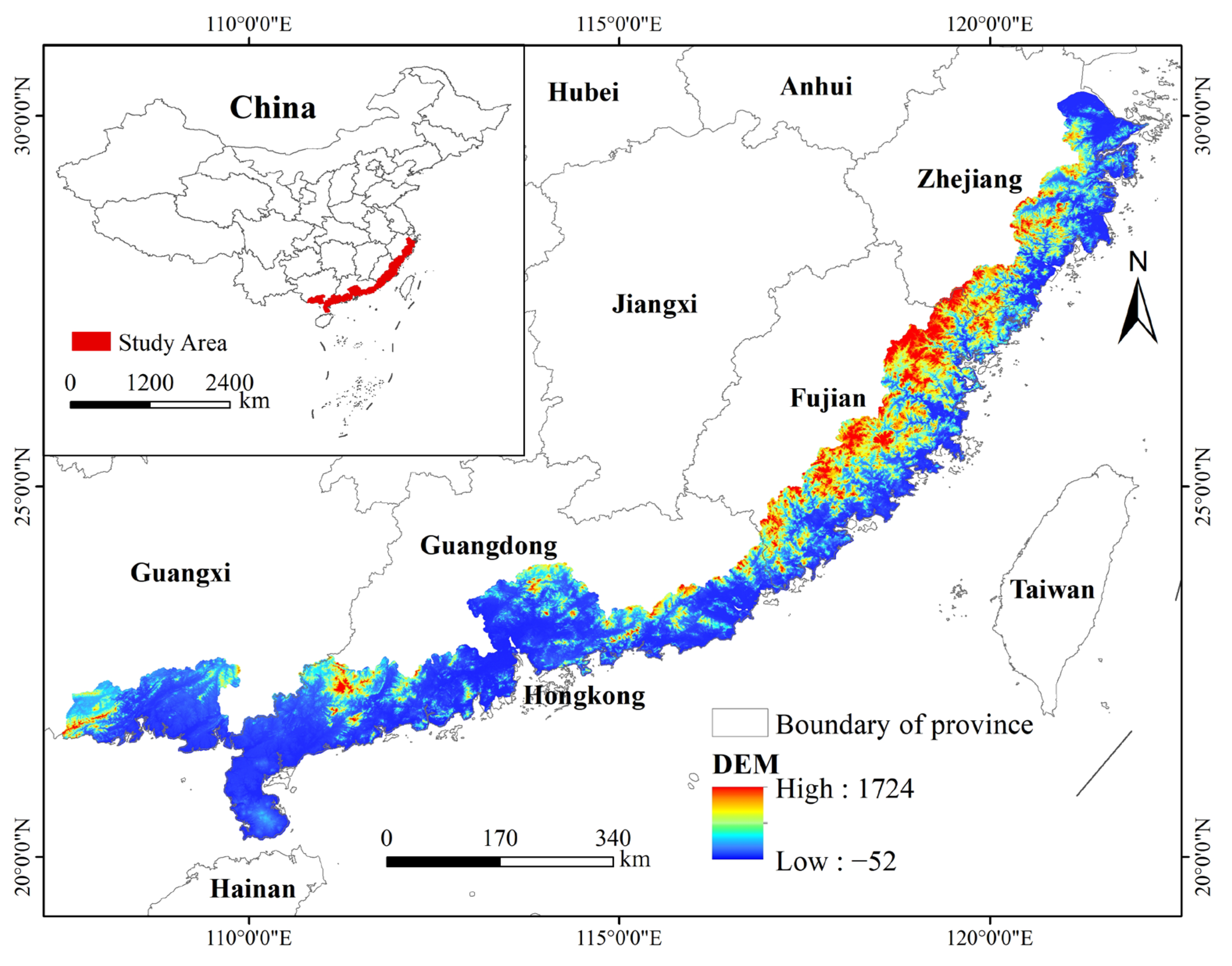
Figure 1. Map of the study area.
Land 14 02101 g001
Figure 2. Technical flow of this study (* means p < 0.05; ** means p < 0.01).
Land 14 02101 g002
Figure 3. The spatial distribution of WY, SC, CS, and HQ at the grid scale throughout the years 2000, 2010, and 2020.
Land 14 02101 g003
Figure 4. Total amount changes in ESs, 2000–2020.
Land 14 02101 g004
Figure 5. The spatial distribution of WY, SC, CS, and HQ at the county scale throughout the years 2000, 2010, and 2020.
Land 14 02101 g005
Figure 6. The spatial distribution of WY, SC, CS, and HQ at the city scale throughout the years 2000, 2010, and 2020.
Land 14 02101 g006
Figure 7. Multi-scale correlation analysis of four ESs from 2000 to 2020. (WY: Water yield, SC: Soil conservation, CS: Carbon storage, HQ: Habitat quality).
Land 14 02101 g007
Figure 8. Bivariate local Moran’s I spatial correlation cluster maps, where (a) is grid scale; (b) is county scale; and (c) is city scale. (WY: Water yield, SC: Soil conservation, CS: Carbon storage, HQ: Habitat quality, HH: high-high synergy, HL: high-low trade-off, LH: low–high trade-off, LL: low-low synergy).
Land 14 02101 g008aLand 14 02101 g008b
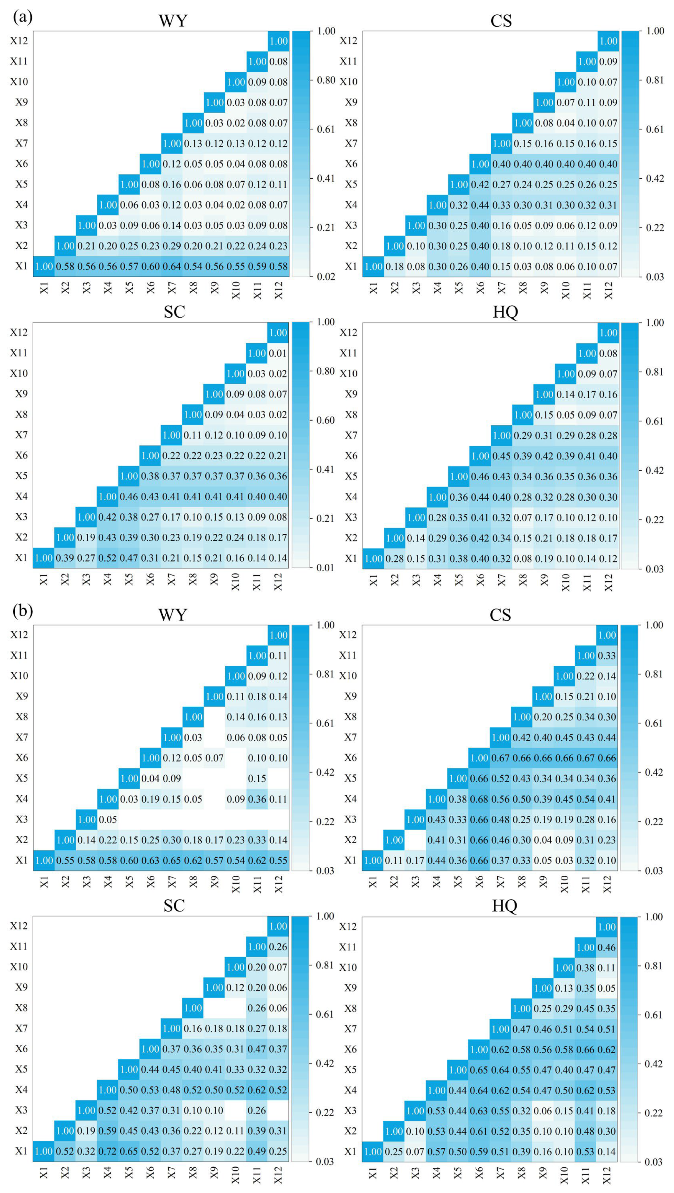
Figure 9. The interaction detection results of multi-scale driving factors on ESs, where (a) is grid scale; (b) is county scale; and (c) is city scale. (X1: Mean annual precipitation, X2: Mean annual temperature, X3: Mean annual evapotranspiration, X4: Slope, X5:DEM, X6: Proportion of forest, X7: Proportion of construction, X8: POP, X9: GDP, X10: Distance from river, X11: Distance from roads, X12: Distance from reserve).
Land 14 02101 g009aLand 14 02101 g009b
Figure 10. LISA clustering maps of ESs and driving factors at the grid scale. (X1: Mean annual precipitation, X3: Mean annual evapotranspiration, X4: Slope, X5:DEM, X6: Proportion of forest, X7: Proportion of construction).
Land 14 02101 g010
Figure 11. LISA clustering maps of ESs and driving factors at the county scale. (X1: Mean annual precipitation, X3: Mean annual evapotranspiration, X4: Slope, X5:DEM, X6: Proportion of forest, X12: Distance from reserve, HH: high-high synergy, HL: high-low trade-off, LH: low–high trade-off, LL: low-low synergy).
Land 14 02101 g011
Figure 12. LISA clustering maps of ESs and driving factors at the city scale. (X1: Mean annual precipitation, X3: Mean annual evapotranspiration, X4: Slope, X5:DEM, X6: Proportion of forest).
Land 14 02101 g012
Figure 13. LULC change in the Research area from 2000 to 2020.
Land 14 02101 g013
Figure 14. Sankey map of LULC transfer changes 2000–2020.
Land 14 02101 g014
Table 1. Sources of data in this research.
DataTypeResolutionData Sources
LULC dataRaster30 mResources and Environmental Sciences and Data Centre, Chinese Academy of Sciences (RESDC) (https://www.resdc.cn/, accessed on 12 June 2024)
River networks data
Reserve data
GDP
Population
Precipitation dataRaster1 kmNational Tibetan Plateau Science Data Center (https://data.tpdc.ac.cn/zh-hans/, accessed on 5 July 2024)
Temperature dataRaster1 km
Evapotranspiration dataRaster1 km
DEMRaster30 mGeospatial Data Cloud (https://www.gscloud.cn/, accessed on 21 June 2024)
Soil dataRaster1 kmHarmonized World Soil Database (https://www.fao.org/, accessed on 30 June 2024)
Table 2. Calculation methods for ecosystem services.
ESsCalculation
Methods
Calculation Method
Water yieldInVEST Model Water Yield Module Y x = 1 A E T x P x × P x
where A E T x   is the actual evapotranspiration of grid cell x ; P x is the rainfall of grid cell x [34].
Soil conservationInVEST Model Soil
Conservation Module
S C = R K L S U S L E
R K L S =   R × K × L S
U S L E = R × K × L S × C × P
where R K L S and U S L E representing the potential erosion amount and the actual erosion. R is the rainfall erosion factor. K is the soil erodibility factor. L S is the slope length factor. C is the vegetation cover and management factor. P is the soil and water conservation factor [35,36,37].
Carbon storageInVEST Model Carbon Module C t o t = C a b o v e + C b e l o w + C s o i l + C d e a d
C a b o v e is aboveground biogenic carbon stock. C b e l o w is belowground biogenic carbon stock. C s o i l is soil carbon stock. C d e a d is dead organic carbon stock [38,39].
Habitat qualityInVEST Model Habitat Quality Module Q x j = H j 1 D x j z D x j z + k z
where H j is the habitat suitability, which takes a value between 0 and 1; D x j is the habitat degradation of grid x in j ; z is the normalization constant, which takes a value of 2.5 [40]; and k is the half-saturation constant, which is usually half the maximum value of habitat degradation [41,42].
Table 3. Detailed information on the sources of driving factors.
TypesDriving FactorsReference
Natural factorsMean annual precipitation (X1)[45]
Mean annual temperature (X2)
Mean annual evapotranspiration (X3)[46]
Slope (X4)[47]
DEM (X5)[48]
Human factorsProportion of forest (X6)[49]
Proportion of construction (X7)
POP (X8)[50]
GDP (X9)[51]
Accessibility factorsDistance from rivers (X10)[52]
Distance from roads (X11)
Distance from reserve (X12)
Table 4. Types of two-factor interaction result.
Judgments BasedInteraction
q ( X 1 X 2 ) < m i n ( q X 1 , q ( X 2 ) ) Weaken, nonlinear
m i n ( q X 1 , q ( X 2 ) ) < q ( X 1 X 2 ) < m a x ( q X 1 , q ( X 2 ) ) Weaken, uni-
q ( X 1 X 2 ) > m a x ( q X 1 , q ( X 2 ) ) Enhance, bi-
q ( X 1 X 2 ) = q X 1 + q ( X 2 ) Independent
q ( X 1 X 2 ) > q X 1 + q ( X 2 ) Enhance, nonlinear
Table 5. The single-factor detection results of multi-scale driving factors on ESs.
q ValueX1X2X3X4X5X6X7X8X9X10X11X12
WYgrid0.7200.0170.2720.0210.0550.0400.1600.0880.0380.0030.0190.003
county0.7750.0010.3310.1800.1580.1530.0420.0890.1110.1030.1690.213
city0.9090.1500.4910.2120.5900.4080.1540.1430.2830.2500.4330.070
SCgrid0.2140.3010.1450.6540.5310.3830.1580.0120.0010.0200.1090.029
county0.3340.0780.0590.6800.9090.5860.3680.1870.0470.0320.3490.082
city0.4070.1580.1480.7590.3520.6540.3060.0670.0560.1310.3630.023
CSgrid0.0590.1480.0520.5450.4240.8650.3630.0850.0250.0230.1270.029
county0.1940.2110.0340.6640.7450.9560.5550.5140.1950.1400.4700.087
city0.4590.4310.2990.8230.7910.9700.6250.5680.4620.1270.7100.180
HQgrid0.0690.1630.0810.4660.3950.5920.3630.0760.0240.0160.1590.028
county0.2030.1900.0110.6390.7280.7780.5960.4770.1730.0820.5440.053
city0.4100.3420.1430.6950.7210.8410.5950.3220.3730.0960.6880.096
(X1: Mean annual precipitation, X2: Mean annual temperature, X3: Mean annual evapotranspiration, X4: Slope, X5:DEM, X6: Proportion of forest, X7: Proportion of construction, X8: POP, X9: GDP, X10: Distance from river, X11: Distance from roads, X12: Distance from reserve).
Table 6. LULC transfer matrixes in the study area from 2000 to 2020.
Land Use and Land Cover Type (km2)Cultivated LandForestGrasslandWater BodyConstruction LandBarelandSum (2020)
Cultivated land43,1172517.1434.8766.951292.951,967.7
Forest1178.692,443.9699.7294.31872.16.196,494.7
Grassland207.7951.111,471.561.2362.42.513,056.4
Water body248142.936.64149.7463.51.55042.2
Construction land632.5254.245.9202.27960.70.39095.8
Bareland4.46.29.76.814.499.9141.4
Sum (2000)45,388.296,315.412,698.25481.115,802.1113.217,5798.2
Disclaimer/Publisher’s Note: The statements, opinions and data contained in all publications are solely those of the individual author(s) and contributor(s) and not of MDPI and/or the editor(s). MDPI and/or the editor(s) disclaim responsibility for any injury to people or property resulting from any ideas, methods, instructions or products referred to in the content.