Article

Voxelized Point Cloud and Solid 3D Model Integration to Assess Visual Exposure in Yueya Lake Park, Nanjing

1
College of Architecture, Nanjing Tech University, Nanjing 211816, China
2
School of Architecture, Southeast University, Nanjing 210096, China
*
Author to whom correspondence should be addressed.
Land 2025, 14(10), 2095; https://doi.org/10.3390/land14102095
Submission received: 23 September 2025 / Revised: 17 October 2025 / Accepted: 17 October 2025 / Published: 21 October 2025

Abstract

Natural elements such as vegetation, water bodies, and sky, together with artificial elements including buildings and paved surfaces, constitute the core of urban visual environments. Their perception at the pedestrian level not only influences city image but also contributes to residents’ well-being and spatial experience. This study develops a hybrid 3D visibility assessment framework that integrates a city-scale LOD1 solid model with high-resolution mobile LiDAR point clouds to quantify five visual exposure indicators. The case study area is Yueya Lake Park in Nanjing, where a voxel-based line-of-sight sampling approach simulated eye-level visibility at 1.6 m along the southern lakeside promenade. Sixteen viewpoints were selected at 50 m intervals to capture spatial variations in visual exposure. Comparative analysis between the solid model (excluding vegetation) and the hybrid model (including vegetation) revealed that vegetation significantly reshaped the pedestrian visual field by reducing the dominance of sky and buildings, enhancing near-field greenery, and reframing water views. Artificial elements such as buildings and ground showed decreased exposure in the hybrid model, reflecting vegetation’s masking effect. The calculation efficiency remains a limitation in this study. Overall, the study demonstrates that integrating natural and artificial elements provides a more realistic and nuanced assessment of pedestrian visual perception, offering valuable support for sustainable landscape planning, canopy management, and the equitable design of urban public spaces.

1. Introduction

In city landscapes, vegetation and water bodies, along with the sky, constitute the most critical natural resources. Through human visual perception, these elements collectively shape the image of the city while simultaneously exerting significant influence on residents’ physical and mental well-being [1], as well as their overall quality of life [1,2]. A substantial body of research in environmental health and environmental psychology provides theoretical foundations for the relationship between human health and urban natural elements. Stress Recovery Theory indicates that exposure to natural settings can trigger rapid physiological and emotional restoration [3], whereas Attention Restoration Theory emphasizes the role of “soft fascination” in mitigating attentional fatigue [4]. Complementary studies on landscape preference and safety further highlight the importance of the prospect–refuge structure in shaping both perceived safety and aesthetic preference [5]. In urban studies, these theoretical perspectives have been operationalized through indicators such as visibility and accessibility, derived from pedestrian perception and behavior, which in turn affect residents’ use of space and health outcomes [6,7].
Pedestrian-level visibility emphasizes visual perception at eye height (1.4–1.6 m), representing a three-dimensional (3D) perspective distinct from traditional two-dimensional (3D) indicators such as viewsheds. Pedestrian-level visual perception more closely reflects everyday experiences and underlies the health mechanisms brought by urban natural elements. In visibility analysis, visual exposure illustrates the potential intensity with which a given object or surface unit is seen from surrounding observation points [8,9]. Visual exposure can be measured, for example, by counts of visibility, visible area, or distance, and is used to evaluate how ‘visible’ a landform or building façade is [10]. Visual exposure is not only a matter of aesthetics but also of equity and public health. Empirical studies have demonstrated significant disparities in street-level greenery across neighborhoods [11,12]. Disadvantaged communities are often “visually deprived” of nature, thereby limiting opportunities for everyday restorative experiences [13,14]. Integrating visibility-based indicators into greenway routing, waterfront access, and view corridor protection can therefore enhance restorative potential and foster a stronger sense of place identity [15]. Collectively, these findings suggest that quantitative research on visual exposure to natural resources offers critical data support for advancing urban sustainability and improving population health. Nevertheless, current research on visual exposure metrics in urban environments remains incomplete, with persistent challenges in multisource data integration and accurate representation of vegetation. In addition, traditional 2D approaches fail to describe increasingly complex and dense urban environments.
Several indicators are mostly used for describing visual exposure to urban natural resources, such as the Green View Index (GVI) and the Sky View Factor (SVF), which have been demonstrated to associate with human health. An increase in street-level GVI has been significantly associated with reduced levels of depression, anxiety, and stress [16,17]. For example, a study in Singapore indicates that if the cumulated GVI within a 100 m buffer increased by one level, the odds of having good mental health would increase by 7.5% [18]. A study in Hong Kong reported that a low value of SVF (under 0.2) can correlate with low land surface temperature, resulting in an increase in thermal comfort degree and easing the urban heat island [19]. In addition, blue spaces with water bodies, due to their unique restorative potential, have also attracted growing attention [20,21]. Moreover, research on urban visual environments has extended beyond natural elements to include artificial components such as building and ground visibility. Early work applied isovist and 3D visibility analysis to examine how building form and mass influence enclosure, openness, and legibility in urban space [22]. More recently, multi-source datasets combined with deep learning and semantic segmentation have enabled high-resolution assessment of visual scenes, identifying buildings, roads, and open surfaces as key components of pedestrian perception [11,23]. These studies highlight the importance of quantifying artificial elements alongside greenery and sky, offering insights into how the built environment shapes spatial experience. However, 2D methods based on imagery or surface elevation vary widely, and effective ways to embed vegetation visibility into comprehensive visual exposure analysis remain limited.
Pedestrian-level visual exposure assessment methods can be broadly categorized into three groups according to the type of data employed: image-based visual analysis, 2.5-dimensional (2.5D) visual analysis, and three-dimensional (3D) model approaches. Image-based indicators primarily describe the proportion of an element occupying the view, including GVI and water–vegetation coverage indices [14]. However, the accuracy of such image-derived measures is often constrained by factors such as shooting angle, shooting time, and image quality. By contrast, 2.5D visual analysis relies on digital elevation models (DEMs) or digital surface models (DSMs) to evaluate viewsheds, the visual enclosure, and spatial complexity [24,25,26], which emphasize the spatial experience from the viewer. Yet, because 2.5D representations cannot fully represent real environments. Complex structures, vegetation morphology, and irregular geometries are often misrepresented in 2.5D models, thereby reducing the accuracy of outcomes. In recent years, advances in remote sensing technologies, such as Light Detection and Ranging (LiDAR) and oblique photogrammetry, have enabled 3D urban spatial models to represent cityscapes with more details and much higher resolution. Point clouds refer to LiDAR-derived collections of discrete 3D points, where each record contains (x,y,z) and radiometric attributes [27]. These data densely sample object surfaces and terrain, allowing more precise quantification of spatial visual characteristics, with recent studies proposing voxelization and ray-tracing techniques to improve computational efficiency [28,29,30]. However, LiDAR point cloud data itself also presents limitations, including incomplete representation of building masses and the difficulty of capturing water surfaces [31]. Different models all have their own advantages and disadvantages. Therefore, a hybrid model could be a solution for quantifying the visual exposure of urban landscapes in detail. Nonetheless, a standardized analytical paradigm for visual assessment based on a hybrid model combining point clouds and other models has yet to emerge.
To address this gap, we develop a hybrid 3D visibility analysis that combines solid models with point clouds, improving both completeness and local detail in pedestrian-level visual metrics and delivering actionable spatial attributes for fine-grained planning and management. By employing line-of-sight ray tracing and voxel sampling in the visibility analysis, point clouds have provided new evidence for elucidating the mechanisms linking natural visibility, spatial morphology, and human well-being [32,33]. Against the trend of rapid urbanization, enhancing the visibility of natural elements and examining the visual proportions of both natural and artificial components in the city can serve as a critical pathway to fostering livable, health-supportive urban spaces and ultimately achieving sustainability. Accordingly, this study aims to develop and validate a pedestrian-scale visual exposure assessment that balances completeness and detail precision, and to use the resulting indicators to diagnose how specific urban elements shape visual conditions in typical waterfront settings.
The remainder of the paper is organized as follows. Section 2 presents the conceptual framework, defines the five line-of-sight–based visual exposure factors, and details the observation simulation using ray casting and voxel sampling, as well as the study area (Yueya Lake, Nanjing), datasets, and model construction. Section 3 reports the results for vegetation-present versus vegetation-removed scenarios and profiles visibility along the lakeside promenade. Section 4 discusses implications for urban planning and management. Section 5 concludes with contributions, limitations, and directions for future research.

2. Materials and Methods

2.1. Study Area and Viewpoint Selection

Nanjing is a high-density modern city, with an urbanization rate of 87.4% as of 2024. This study selects the Southern area of Yueya Lake Park, located in Qinhuai District, Nanjing, as the research site. The park is bordered on the west by a section of the city wall and surrounded by dense buildings to the east (Figure 1). Located in a high-density urban environment, Yueya Lake Park offers superior natural resources and a diverse mix of natural and artificial elements, alongside well-established greenery.
The lake, crescent-shaped in form, covers an area of 17.2 hectares. Yueya Lake Park is divided into two major zones, north and south, by Hou Biaoying Road, with a total area of approximately 36.2 hectares, where the Southern area covers 15.3 hectares. Vegetation within the park is planted in a carefully layered arrangement, with a well-balanced mix of trees and shrubs. Tall trees are planted along most of the park’s pathways, creating shaded promenades. Due to its geographic location, the expansive water surface of Yueya Lake provides broad and open views. Compared with the northern section, the southern section has better greening and a denser surrounding built environment, combining high urban density with high greenery, which makes it an appropriate study area for this research. In the Southern area, the main park road is a north–south route approximately 5 m wide, complemented by a secondary pathway, a circular lakeside promenade about 2 m wide. Visitors in the park can enjoy sweeping vistas of Purple Mountain while walking along the city wall to experience its historic atmosphere and simultaneously gain refreshing and restorative visual contact with the surrounding natural landscape.
The centerlines of the park roads in the southern sections were digitized, and observation points were extracted at 50 m intervals along these routes. Each viewpoint was assigned a terrain elevation value, with an additional 1.6 m added to represent eye height. As noted earlier, the southern section of the park is predominantly linear, with one waterside pathway extending southward with a length of 751 m. The viewpoints represent pedestrian-level visual perception and were located along the waterside pathway in the southern area of Yueya Lake Park. To simulate walking experiences, viewpoints were placed at 50 m intervals, resulting in 16 evenly distributed points. This strategy provides continuous coverage of the pedestrian perspective along the promenade. The selected viewpoints were numbered sequentially from south to north (1–16), and their spatial distribution is illustrated in Figure 1.

2.2. Urban Hybrid Model Construction

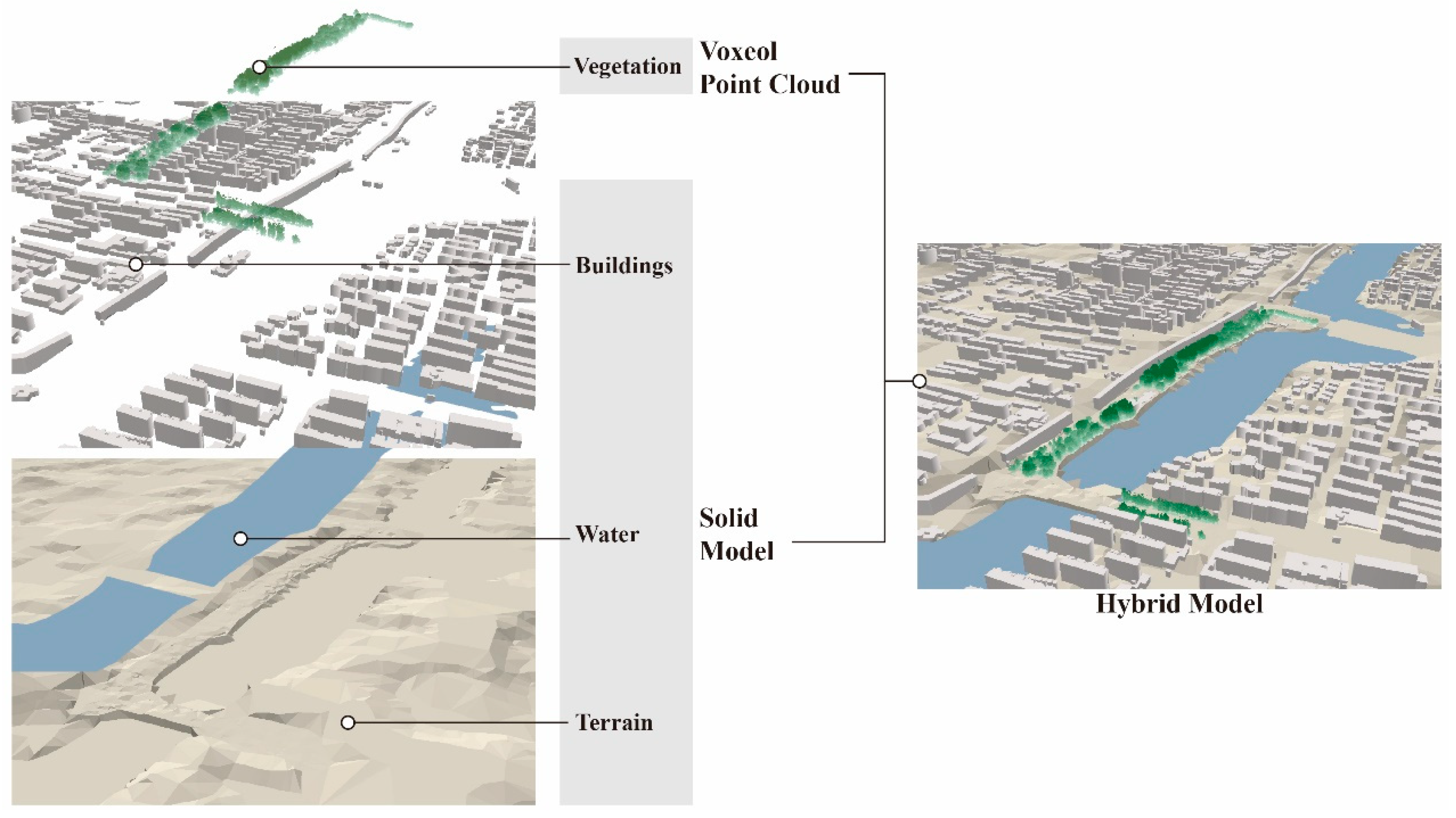
This study proposes a hybrid modeling framework that integrates solid models with point cloud data (Figure 2), primarily implemented on the ArcGIS Pro platform. The DEM, building footprints, and point cloud were spatially registered via projection alignment and manual control-point matching.
The solid model consists of a terrain DEM, building solid models, and water surface models. DEM with a resolution of 30 m was generated from the Geospatial Data Cloud (https://www.gscloud.cn/, accessed on 1 September 2024). The building solid models were constructed from the Baidu Map building footprints with height and floating on the DEM. Conventional buildings are modeled in Level of Detail 1 (LOD1) by extruding building footprints to their respective heights on top of the ground elevation with the extrusion function embedded in ArcGIS Pro [34]. In LOD1, each building is represented as a simple prismatic volume obtained by extruding its footprint to the recorded building height on top of the local ground elevation, with no roof geometry, façade details, windows, or textures [35]. In ArcGIS Pro (version 3.4), LOD1 building models were created by extruding building footprint polygons to their recorded heights with the DEM as the ground reference [34]. Water surface models were represented as a 3D surface above the DEM with the normal water level. Therefore, the solid model can be classified into three categories, namely ground, buildings and water bodies.
Vegetation is represented using voxelized point cloud data. We collected mobile LiDAR data using a ZEB-HORIZON handheld 3D laser scanner (GeoSLAM, UK). The initial point cloud includes all scene elements (ground, vegetation, buildings, and miscellaneous objects). Raw data were saved in LAZ format, totaling about 4.57 GB with more than 400 million points and an accuracy of approximately 1 cm. Vegetation points were then extracted and voxelized, yielding a LAZ file of 104 MB containing 5,326,029 points.
Since the vegetation point cloud data is an irregular structure, which is difficult to transfer into a solid model, the raw point cloud is voxelized to generate a voxel-based model, which allows for efficient representation and calculation of volumetric vegetation structures. Finally, all models are spatially aligned through coordinate registration, enabling the integration of DEM-based terrain, LOD1 building solids, and voxelized vegetation into a single hybrid model.

2.3. Hybrid-Model-Based Visibility Analysis

This study primarily employs line-of-sight (LoS) analysis to evaluate visibility from the pedestrian perspective. The LoS analysis comprised three main steps (Figure 3): (A) generating quasi-spherical 3D line segments to simulate the human field of vision, (B) performing preliminary visibility analysis with the solid model using quasi-spherical 3D line segments, and (C) finally incorporating these rays into the vegetation voxel model to determine whether they were blocked by vegetation.
First, viewpoint locations were selected, and an eye-level height was assigned, as introduced in Section 2.1. To simulate human vision, the horizontal field of view was set to 360°, capturing the complete panoramic range around the observer. For the vertical field of view, a range of −30° to 90° was selected (0° = visual plane). The simulation of human vision space can be seen in Figure 3a. From each viewpoint, a set of uniformly distributed three-dimensional rays was generated in a spherical pattern with a certain LoS length of 1000 m within the medium-distance view as defined by Higuchi [36].
In this study, the angular resolution of LoS ray sampling was set to 3° in both the horizontal and vertical directions. This means that rays were emitted every 3° horizontally across the full 360° field of view and every 3° vertically within the −30–60° vertical range. With this setting, each viewpoint produces 3388 rays, which collectively represent a discretized approximation of the pedestrian visual field. These rays serve as the basis for calculating visual exposure indicators. Each LoS ray is also treated as a pixel within the simulated visual scene, thereby allowing the discretization of the pedestrian field of view into quantifiable units and used to visualize the view.
By constraining the vertical angle, the analysis reduces the influence of ground surfaces and low-angle occlusions that provide limited environmental information, thereby aligning the simulated view more closely with natural human perception. Within this defined visual envelope, rays were cast at equal angular intervals to generate a dense three-dimensional sampling grid. The density of LoS rays was chosen to balance computational efficiency with visual accuracy, ensuring sufficient resolution to capture fine-scale elements such as vegetation canopies and building edges. This configuration allows for the identification of objects intersecting with each ray, enabling the classification of visible elements.
All visibility computations were executed within a single Python (version 3.12) workflow, with ArcGIS Pro functions called via the arcpy library to perform Line of Sight (LoS) analysis on the LOD1 solid model (Figure 3b). Based on the visible LoS rays identified in ArcGIS Pro, a voxel-based LoS ray analysis was subsequently performed in Python. The pseudocode of the LoS analysis can be found in Appendix A.1. In this step, each voxel point was represented as a cube with a side length of 100 mm. During the voxel-based analysis, each ray was evaluated to determine whether it was obstructed by any voxel cube (Figure 3c). The final results represent the set of LoS rays that remain visible after accounting for both the solid model and the vegetation voxel model.

2.4. Visual Exposure Indicators

We simulate pedestrian vision at eye height (1.5 m) along the lakeside promenade using a line-of-sight (LoS) ray-casting scheme against a hybrid 3D model. Rays are generated from each viewpoint at fixed angular steps; each ray is labeled by the class of its first intersection (or “sky” if no hit). This produces a perception-consistent, ground-level map of what a person would visually encounter in situ. In this study, five key visual exposure indicators were proposed to jointly describe natural and artificial elements in the simulated urban visual scene, all derived directly from the LoS ray classifications. Natural elements are represented by the Green View Factor (GVF), Sky View Factor (SVF), and Water View Factor (WVF), which quantify the proportions of vegetation, sky, and water bodies visible within the pedestrian’s field of view. Artificial elements are described by the Building View Factor (BVF), indicating the proportion of built structures, and the Ground View Factor (GRDVF), representing the proportion of ground surface visible in the visual scene. Together, these indicators provide a comprehensive framework for quantifying visual exposure in urban environments from the pedestrian perspective.
All the indicators are derived from hybrid-model-based visibility analysis, which simulates human visual fields by recording the categories of objects that obstruct or appear within the view based on the hybrid model. The GVF represents the proportion of visible green vegetation; the SVF denotes the proportion of sky within the view, calculated from rays that are not obstructed by objects; the WVF reflects the proportion of large water bodies such as ponds, lakes, or rivers visible within the view.
To quantify the five visual exposure indicators, LoS rays were classified according to the type of object they intersected:
N t o t a l : the total number of LoS rays generated from a viewpoint, which equals 3388 in this case;
N G r e e n : the number of rays intercepted by vegetation;
N W a t e r : the number of rays intercepted by water bodies;
N i n t e r v i s i : the number of rays unobstructed by any object, which terminate at the sky;
N B u i l d i n g : the number of rays intercepted by buildings;
N G r o u n d : the number of rays intercepted by the ground.
Following the above definitions, the proposed visual exposure indicators were then defined and calculated as shown in Table 1 with references.

2.5. Visual Distance

It is noteworthy that using LoS rays in a 3D model not only enables the calculation of the proportion of each visual element within the field of view but also provides the direct distance from the observer to each visible element. The distance between an element in the urban environment and the observer may influence human experience [42]. This measurement, defined as visual distance in this study, allows the analysis to capture not only the relative composition of visual exposure but also the spatial depth structure of the pedestrian visual environment. Visual distance refers to the mean linear distance between the observer (viewpoint) and the first intersected object along a LoS ray in three-dimensional space. It captures the spatial depth of visible elements within the urban environment and provides insight into whether visual exposure is dominated by foreground, middle-ground, or background features. Unlike visual ratios, which measure the proportion of each element within the field of view, visual distance quantifies the depth distribution of those elements. The visual distance for element i of a viewpoint j is defined as:
V D i j = 1 N i j k = 1 N i j d i j , k
where N i j is the number of LoS rays intersecting element i, d i j , k is the Euclidean distance from viewpoint i to the intersection point of the LoS ray k, i.e., the length of the ray.

3. Results

3.1. The Visual Exposure and Visual Distance

In this study, both the solid model (without vegetation) and the hybrid model (with vegetation) were processed in the same case, allowing for a clear demonstration of the differences and advantages of the proposed method. The original result of the number of LoS rays ended with different landscape elements is represented in Appendix A.2. Table 2 and Table 3 represent the results showing clear patterns in visual exposure composition and visual distance across the selected 16 viewpoints, respectively. The comparison directly reveals significant differences in the distribution of visual exposure indicators and visual distance. From a methodological perspective, explicitly incorporating vegetation ensures that the model captures canopy occlusion, porosity, and near-field enclosure effects. Without vegetation, visibility assessments are biased toward buildings and sky, leading to incomplete or misleading interpretations of urban visual environments. The hybrid model addresses this gap by providing a more realistic representation of spatial hierarchy and depth.
Table 2 summarizes the value (%) of GVI, SVF, WVF, BVF, and GRDVF for all 16 viewpoints under the two modeling strategies. Across 16 viewpoints, adding vegetation voxels (Hybrid) substantially reshaped visual exposure. For the solid model, vegetation was excluded, so GVI = 0 in the solid model. In contrast, the hybrid model integrates vegetation, resulting in vegetation dominating visual exposure and simultaneously reducing SVF and BVF. SVF declined from 50.19% to 21.62%, with an average change of −28.57 percentage points. WVF was relatively stable, shifting from 6.89% to 6.14%, a change of −0.75 (SD 0.9). BVF decreased from 17.62% to 1.98%, with a change of −15.64. GRDVF increased from 25.31% to 27.44%, with a change of +2.13. VP13 shows an extreme illustrated pattern: GVI ranged from 6.38% (VP6) to 74.68%, while the strongest SVF reduction occurred (−50.18%). WVF exhibited low dispersion in both models, consistent with limited vegetation occlusion of lake views along most segments. Overall, vegetation markedly reduces sky and building visibility, has minimal effect on water views, and elevates green exposure, producing a more nature-forward visual field along the promenade.
Table 3 reports visual distances (m) for vegetation, ground, water, and buildings. Because Sky is determined by the criterion of no obstruction, all LoS rays reaching the sky are assigned the maximum threshold distance of 1000 m. As this value is constant and does not reflect actual spatial variability, Sky is excluded from the computation and discussion of visual distance. Instead, the analysis focuses on vegetation, ground, water, and buildings, which vary dynamically in both proportion and distance across viewpoints.
Vegetation appears only in the Hybrid model, with a mean viewing distance of 12.76 m, indicating that greenery is generally perceived at close range. The visual distance of water reduced from 78.06 m in Solid to 71.74 m in Hybrid, an average change of −6.32 m, showing mild near-shore occlusion by vegetation. In contrast, buildings shift farther away when vegetation is included. Noting that SD for the building distance difference (Hybrid − Solid) has a high value of 73.665, reflecting mixed occlusion regimes and sampling imbalance. When vegetation is involved, from some viewpoints, many façades in the median range (90–120 m) are blocked by the greenery, and only several building rays with very near or far distances remain. This effect is strongest at VP4, VP11, VP13, and VP16, resulting in a high value of SD. Ground distances drop from 22.45 m to 11.93 m, a mean change of −10.52 m, consistent with reduced long, low-angle sightlines under canopy and a shift toward nearer ground patches. Overall, vegetation draws the visual field inward for ground and slightly for water, while pushing the building horizon outward, and it introduces a close-range green layer that dominates near-field perception along the promenade. The value of differences highlights how vegetation reshapes spatial depth. In the hybrid model, vegetation dominates the foreground (≤40 m), while ground and water shift to the middle field (>50–300 m), and buildings retreat further into the far field (>150–400 m).

3.2. The Comparison Between the Solid and Hybrid Models

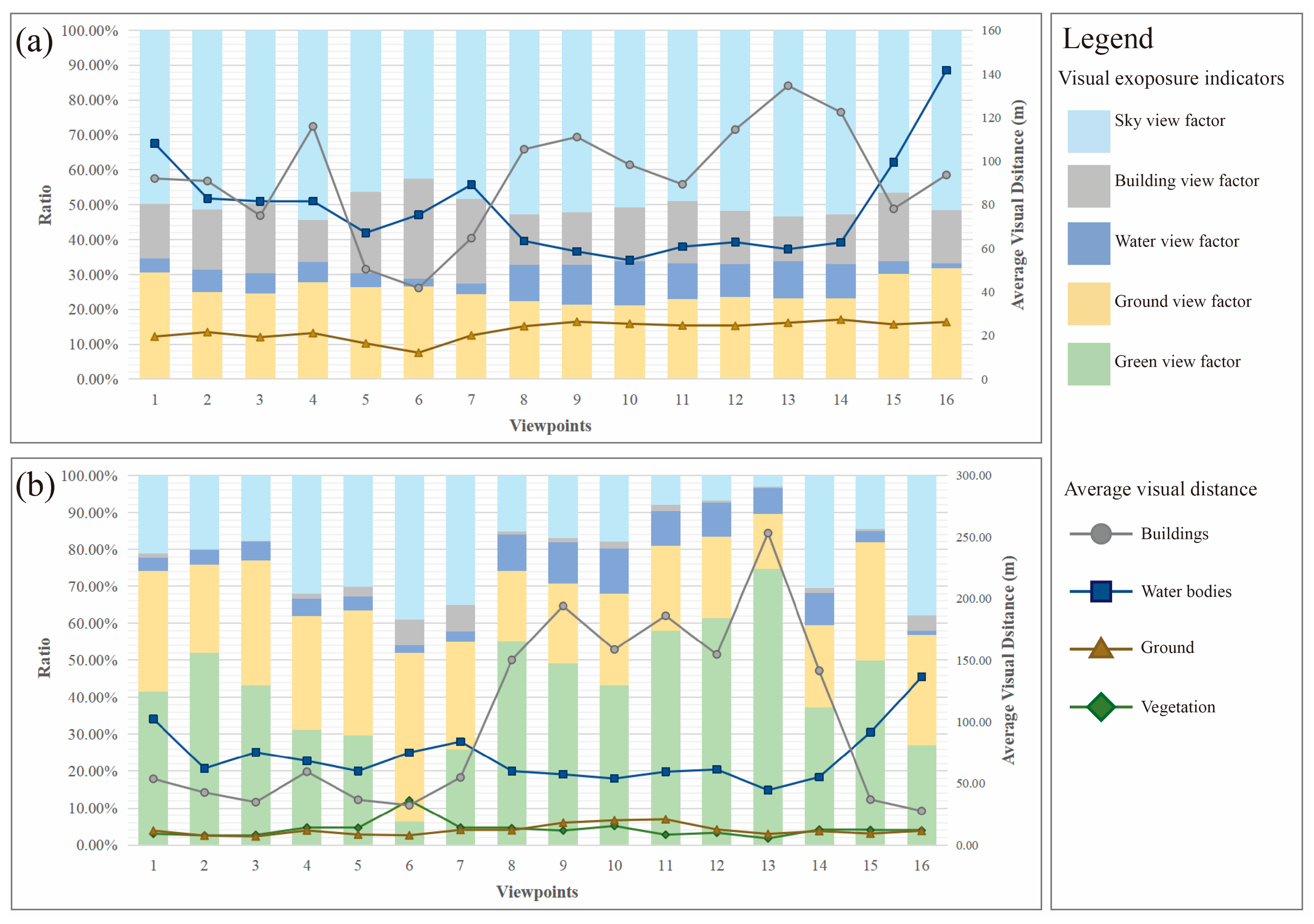
Figure 4 presents the visual exposure results for viewpoints 1–16 along the lakeside promenade from south to north, based on the solid model without vegetation and the hybrid model with vegetation. Together with the data shown in Table 2 and Table 3, the comparison highlights how vegetation reshapes both the proportional composition and the spatial hierarchy of pedestrian visual perception.
In the solid model, sky visibility remained dominant, accounting for 42.62–54.40% of the visual field, reflecting the openness of the promenade in the absence of vegetation. Ground contributed 21.22–31.70%, with higher ratios at the southern end (viewpoints 15–16) where paths are wider, and lower ratios near the lakefront in the north. Buildings (walls and structures combined) accounted for 10.21–25.55%, typically perceived at middle to far distances (198.64–415.42 m), with closer walls (30.02–59.69 m) providing immediate enclosure. Water varied from 1.56% to 11.51%, usually appearing at mid-range distances (54.53–108.07 m). Overall, the solid model shows a layered structure with ground and walls in the foreground, water and nearby buildings in the mid-field, and sky as the dominant background.
In contrast, the hybrid model revealed a significant shift with the inclusion of vegetation. GVI emerged as the dominant element across most viewpoints, ranging from 6.38% (viewpoint 6) to 74.68% (viewpoint 13), and was consistently perceived in the near field (5.37–36.33 m), serving as the primary enclosure of the visual space. SVF displayed pronounced variability (3.10–38.93%), in contrast to the more stable proportions observed in the solid model, which can be attributed to the diverse canopy structures and rich vegetation coverage within the park. WVF ranged from 1.24% to 12.22%, concentrated in the middle segment (viewpoints 8–12), and was perceived at mid-range distances (44.64–136.56 m). Artificial elements became less prominent: BVF remained below 7.17% with distances of 27.67–253.11 m, while GRDVF contributed 14.87–45.60% in the near field (6.99–20.82 m).
In summary, the comparison between the solid and hybrid models reveals two key aspects of change. First, in terms of visual exposure indicators, sky visibility dropped sharply from an average of 49.76% to 21.10%, while ground visibility declined from 26.47% to 23.03%. Buildings decreased significantly from 17.55% to 2.93%, whereas vegetation, which was absent in the solid model, emerged as the dominant category, averaging 42.93%. Water visibility remained relatively stable, though its role shifted as it became more frequently framed by vegetation. Together, the green and blue view factors occupy almost half of the visual field, suggesting a visually supportive environment enriched by natural elements. Second, the visual distance results confirm a restructuring of depth. Vegetation appeared as the nearest layer with an average viewing distance of 12.76 m, compressing the foreground and reducing visible ground depth from 22.45 m to 11.93 m. Buildings shifted outward, with mean distances increasing from 92.37 m to 101.08 m, while water remained a mid-field feature, decreasing slightly from 78.06 m to 71.74 m.
Spatially, the southern segment (viewpoints 1–5) presented balanced exposure between vegetation, sky, and ground. The middle segment (6–12) was dominated by vegetation and water, creating a strong contrast between near- and mid-field layers. And the northern segment (13–16) displayed higher variability, with vegetation and ground alternately shaping the foreground. Overall, the hybrid model demonstrates that vegetation fundamentally restructures the urban visual environment in Yueya Lake Park, reducing the dominance of sky and ground while enhancing enclosure and depth through near-field greenery.

3.3. Typical View Visualization

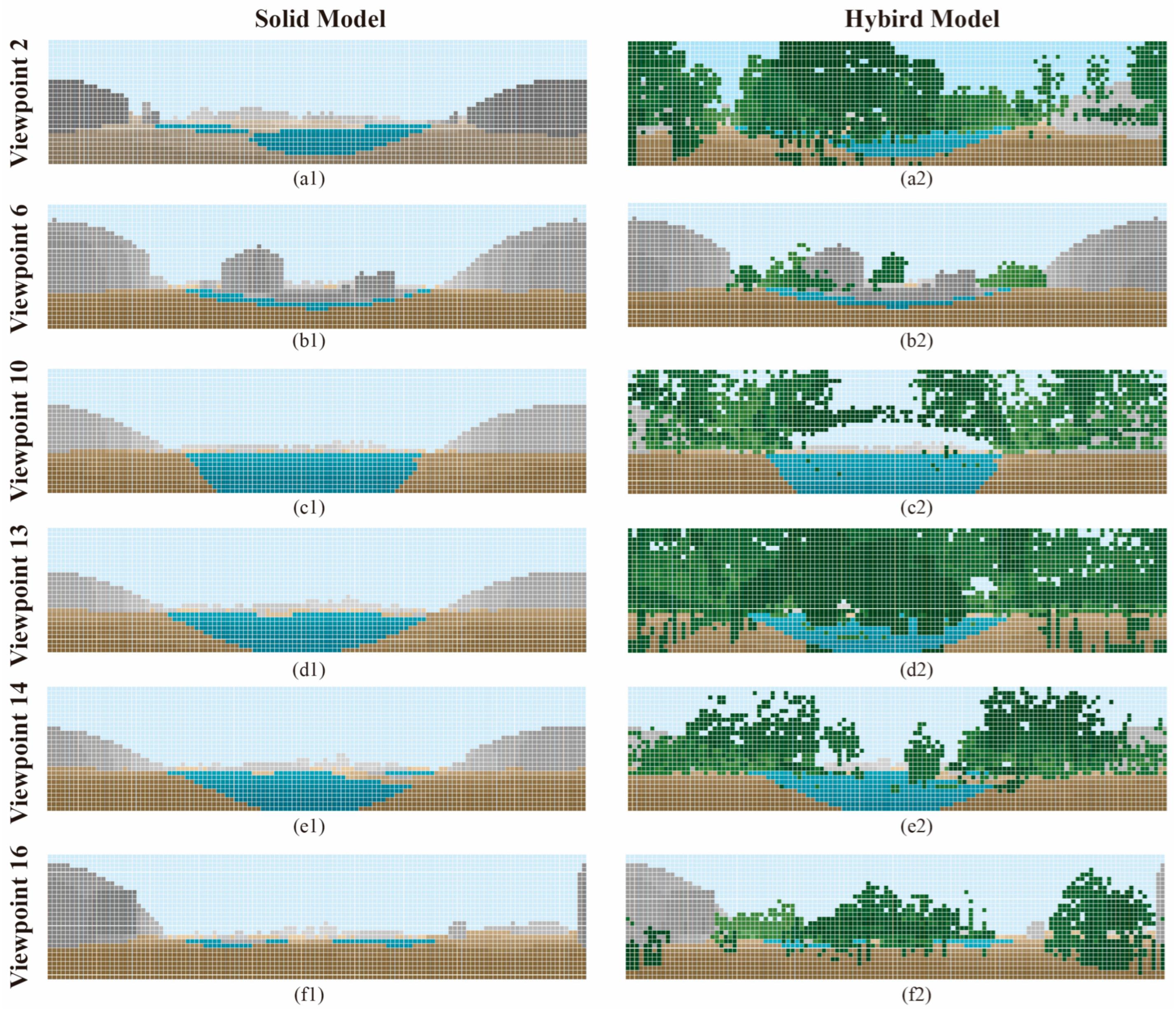
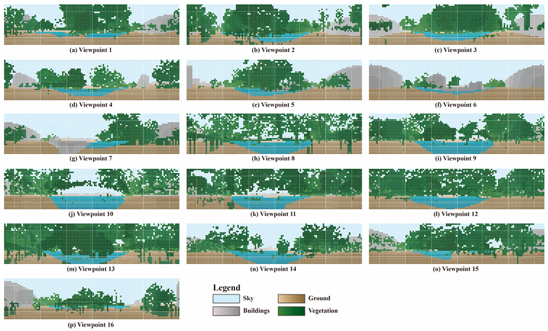
Based on the analysis of the 16 viewpoints, several positions can be identified as representative examples that capture the diversity of pedestrian visual experiences along the southern promenade of Yueya Lake Park. Visualization of all viewpoints can be seen in Appendix A.3. Figure 5 presents a comparison between the solid model (left) and the hybrid model (right) across six representative viewpoints (VP2, VP6, VP10, VP13, VP14, and VP16). The contrast highlights how the inclusion of vegetation substantially reshapes the pedestrian visual environment.
Within the solid model, buildings and ground surfaces together accounted for an average of 42.93% of the pedestrian visual field. In contrast, the integration of vegetation within the hybrid model results in marked shifts in visual composition, as tree canopies block a considerable portion of building views in both the foreground and middle ground. Vegetation occupies a large share of the near- and mid-field, reducing the visible proportion of sky and buildings, while also reframing water views through canopy openings. For example, VP13 shows how dense vegetation produces a “green tunnel” effect in Figure 5(d2), while VP16 illustrates the partial reopening of views toward distant landscape features in the northern section in Figure 5(f2).
At the southern entrance (Figure 5(a2)), the views are relatively balanced, with moderate contributions from vegetation (around 40–52%) and ground (>20%), providing a useful baseline condition for comparison. Moving northward, VP6 stands out as an extreme case with the lowest GVI (6.38%) and the highest SVF (38.93%), accompanied by elevated BVF (7.02%), which can be seen in Figure 5(b2). This viewpoint faces a building to its east, blocking most views of water bodies, illustrating a section with sparse canopy coverage where sky and built structures dominate. In contrast, VP13 represents the opposite extreme (Figure 5(d2)), with the highest GVI (74.68%) and the lowest SVF (3.10%), indicating a highly enclosed “green tunnel” effect where vegetation overwhelmingly shapes the visual field.
The promenade also includes sections where water exposure becomes prominent. At VP10 (Figure 5(c2)), WVF reaches its highest values (12.22%), highlighting how the lake becomes a mid-range focal point framed by vegetation. Further north, VP14 demonstrates another turning point (Figure 5(e2)), where SVF rises again (30.61%) while GVI decreases to 37.19%, reflecting a partial opening in the canopy and a stronger sense of spatial openness. VP16 is located in the northern entrance (Figure 5(f2)), with moderate GVI (26.98%) and relatively high SVF (37.87%), indicating a more open and distant perspective.
Together, these representative viewpoints, namely VP2 (baseline), VP6 (low vegetation, high sky), VP10 (water-focused), VP13 (high vegetation enclosure), VP14 (sky re-opening), and VP16 (baseline), capture the range of visual patterns along the route. They effectively illustrate the transitions from balanced entrance views to canopy-dominated enclosures, framed lake vistas, and localized openings, thus providing a coherent narrative of spatial change in the pedestrian visual experience.
This comparison indicates the necessity of incorporating vegetation in visibility analyses. Ignoring vegetation risks overestimates sky openness and ground exposure while underestimating the immersive enclosure provided by greenery, which is critical for understanding pedestrian-level visual experience and health-related outcomes.

4. Discussion

4.1. Advantages of the Proposed Hybrid-Model-Based Visibility Analysis

The proposed hybrid-model-based visibility analysis offers several methodological and practical advantages compared with traditional approaches. First, integrating solid 3D models with voxelized vegetation point clouds yields a more realistic joint representation of natural and artificial elements and enables more accurate assessment of how greenery shapes visual environments. Conventional visibility analysis often neglects vegetation or relies on simplified geometric proxies. Previous studies have shown that oversimplified vegetation proxies, such as spherical or cylindrical crowns, may produce unreliable outcomes and deviate from real-world conditions [31]. By contrast, the visual patterns revealed in this study indicate that the hybrid model captures canopy porosity, irregular morphology, and occlusion in ways that narrow the gap between simulation and pedestrian perception. This aligns with voxelized forest evidence [43].
Second, the framework provides pedestrian-oriented visibility metrics that directly reflect the experiential quality of urban spaces. By adopting LoS sampling, the method not only quantifies the visual exposure of natural and built elements but also records their visual distances, offering richer insights into spatial depth and perceptual accessibility. Recent advances demonstrate that point cloud data enables accurate and high-resolution representation of vegetation and urban structures [44,45], further supporting the reliability of this approach.
Third, this method contributes to sustainable urban management by linking perceptual data with planning decisions. For instance, it allows planners to identify areas where greenery is visually underrepresented, to evaluate the effectiveness of view corridor protection, and to optimize the placement of vegetation for both ecological and psychological benefits. This study presents a side-by-side with and without vegetation workflow that makes planting impacts explicit, informs planning, and reveals when density undermines visual goals. Paired models guide selective pruning, thinning, or removal, reducing canopy or understory to expand water views, while preserving landscape quality and targeting specific trees. At the same time, the hybrid model supports LOS-based visualization, enabling a transparent and communicable way to present the perceptual impacts of planning interventions to policymakers and the public.
Together, these advantages highlight the potential of hybrid-model-based visibility analysis as a reliable and applicable tool to support livable, equitable, and health-supportive cities.

4.2. The Potential Usage in Sustainable Research

The hybrid model developed in this study, which integrates solid 3D city models with point cloud-derived vegetation, provides a novel perspective for visibility analysis in urban environments by taking real shapes of vegetation into account. This methodological advancement holds significant implications for sustainable urban research.
First, it links ecological functions of vegetation with visual-spatial experience, demonstrating that trees and canopies not only regulate microclimates and sequester carbon but also reshape perceptual exposure to green and blue elements. These visual exposures are closely tied to mental health, stress recovery, and cognitive restoration, suggesting that urban sustainability should integrate perceptual well-being alongside ecological metrics [7,46]. Second, the hybrid-model-based visibility analysis provides a diagnostic tool for urban regeneration projects. By quantifying how vegetation alters the balance of green, sky, water, building, and ground views, planners can identify where restorative visual resources are lacking and prioritize interventions that improve both ecological and perceptual sustainability. This aligns with contemporary sustainable design paradigms that emphasize human-centered urban spaces, where livability and well-being are considered key outcomes of spatial planning. Third, linking visual exposure indicators with health data provides actionable evidence for health-oriented planning. For instance, consistent with Attention Restoration Theory and Stress Recovery Theory, segments with higher GVF and stable WVF can support positive mental status [47,48,49]. Using the hybrid model supported visibility analysis, multiple indicators proposed in this study can be integrated with health datasets to explore spatial configurations that better support healthy cities. Finally, this approach enables a more equitable vision of sustainability. The ability to measure visual exposure at fine spatial scales means disparities in access to natural views can be identified across neighborhoods. Ensuring that all social groups benefit from restorative visual resources can help address inequalities in urban health and quality of life.

4.3. Limitations and Future Work

A major limitation of this study lies in the computational efficiency of line-of-sight analysis with the solid model in ArcGIS. Specifically, a single viewpoint with 3388 LoS rays extending 1000 m required approximately 3–4 h of processing time in this study. By contrast, visibility analysis with the voxelized point cloud model took less than one minute for a single viewpoint, demonstrating a dramatic improvement in computational efficiency. When the number of viewpoints or the complexity of the solid model increases, the computational burden in ArcGIS grows exponentially, making large-scale or city-wide applications impractical under the current workflow. This performance bottleneck highlights the need for more efficient algorithms or alternative software environments.
Future work could incorporate parallel computing strategies, GPU acceleration, or more lightweight 3D spatial analysis libraries to reduce processing time. In addition, hybrid workflows that combine ArcGIS with external Python-based ray-tracing packages or open-source 3D engines may offer opportunities to optimize performance while retaining analytical accuracy. Furthermore, more case studies can be expected by adopting the proposed method for exploring a wider range of visual characteristics, which would contribute to a better understanding of the complexities of urban environments.

5. Conclusions

This study introduced a hybrid-model-based approach for quantifying pedestrian-level visual exposure by combining solid 3D models with voxelized point cloud vegetation. Unlike traditional models that either omit or oversimplify vegetation, the hybrid model more realistically represents natural elements, thereby improving the accuracy of visibility analysis. Applied to Yueya Lake Park in Nanjing, China, the method evaluated five visual exposure indicators reflecting the visual characteristics of both natural and artificial elements in urban environments. Results revealed that vegetation significantly reshapes both the proportion and distance of visible elements, underscoring its decisive role in shaping urban perceptual experiences. These findings confirm that explicitly considering vegetation reduces deviations between simulation and real-world perception, while enhancing the reliability of urban visibility studies.
The proposed method advances urban spatial analysis by addressing the limitations of conventional 2D approaches and overly simplified vegetation models. Beyond methodological innovation, the framework also demonstrates practical value for sustainable urban planning. By quantifying and visualizing areas with natural views, protecting key visual corridors, and optimizing vegetation placement, planners are able to better integrate ecological and psychological benefits into urban regeneration strategies. Moreover, the method directly contributes to the Sustainable Development Goals (SDGs) by providing data-driven support for sustainable landscape planning, effective greenery and canopy management, and equitable urban design that enhances both environmental performance and human well-being. Despite limitations in computational efficiency, especially within ArcGIS-based LoS analysis, the voxelized hybrid approach demonstrates considerable potential for practical application. Future applications should extend this method to diverse urban contexts and dynamic scenarios, ensuring that visibility analysis contributes to livable, equitable, and health-supportive cities.

Author Contributions

Conceptualization, G.Z.; methodology, G.Z.; software, G.Z. and S.C.; validation, G.Z., D.Y. and S.C.; formal analysis, G.Z.; investigation, D.Y.; resources, G.Z.; data curation, G.Z.; writing—original draft preparation and revision, G.Z., D.Y. and S.C. All authors have read and agreed to the published version of the manuscript.

Funding

This research was funded by the National Natural Science Foundation of China (Nos. 52108045, 52408067, 52578065); Fundamental Research Funds for the Central Universities (No. 2242021R20016); Jiangsu Planned Projects for Postdoctoral Research Funds (No. 2021K024A); China Postdoctoral Science Foundation, (Nos. 2021M700767, 2022T150115); The Scholarship for Visiting Scholars of Key Laboratory of New Technology for Construction of Cities in Mountain Area (No. LNTCCMA-20240106) and China Scholarship Council (No. 202206090038).

Institutional Review Board Statement

Not applicable.

Data Availability Statement

The datasets presented in this article are not readily available because the data are part of an ongoing study. Requests to access the datasets should be directed to the corresponding author.

Conflicts of Interest

The authors declare no conflicts of interest.

Abbreviations

GVFGreen View Factor
SVFSky View Factor
WVFWater View Factor
BVFBuilding View Factor
GRDVFGround View Factor
LoSLine of Sight
DEMDigital elevation model

Appendix A

Appendix A.1. Pseudocode of the LoS Analysis Based on the Hybrid Model

 INPUTS:
  V = {v1, v2, …}         # viewpoints at eye height 1.5 m along promenade
  Δaz = 3°, Δel = 3°          # angular resolution
  AZ_RANGE = [0°, 360°)        # full azimuth
  EL_RANGE = [−30°, 60°]         # constrained elevation
  SOLIDS = {water, buildings}       # LOD1 solid models (multipatches/3D features)
  DEM = {ground}           # digital elevation model for terrain
  VOXELS = {cubes, size = 0.1 m}    # vegetation voxel model
  CLASSES = {vegetation, sky, water, building, ground}  # mutually exclusive
  OBSERVER_HEIGHT = 1.5 m
  OUTPUT_DIR = path
 # ------------------------------------------------------------
 # Utility: spherical grid of ray directions
 # ------------------------------------------------------------
 FUNCTION BUILD_RAY_DIRECTIONS(Δaz, Δel, AZ_RANGE, EL_RANGE):
  DIRS = []
  ray_id = 0
  FOR el FROM EL_RANGE.min TO EL_RANGE.max STEP Δel:
   FOR az FROM AZ_RANGE.min TO AZ_RANGE.max STEP Δaz:
    DIRS.append({id: ray_id, vec: UNIT_VECTOR_FROM_AZ_EL(az, el),
          az: az, el: el})
    ray_id = ray_id + 1
   RETURN DIRS
 # Expected |DIRS| ≈ 3388 with the given angular settings
 # ------------------------------------------------------------
 # ArcGIS Pro (arcpy): per-ray LoS on SOLIDS + DEM
 # Returns first-hit class and distance for each ray
 # ------------------------------------------------------------
 FUNCTION ARCPY_LOS_SOLIDS_DEM(viewpoint v, DIRS, SOLIDS, DEM, OBSERVER_HEIGHT):
  # 1) Build a temporary feature class of rays in the geodatabase
  rays_fc = ARCPY_BUILD_RAY_FEATURES(v, DIRS, OBSERVER_HEIGHT)
  #  - Create a 3D line for each ray: start = v.position,
  #   end = v.position + RAY_MAX_RANGE * DIR.vec
  #  - Store ray_id as attribute
  # 2) Run line-of-sight against DEM and LOD1 solids
  #  Using the arcpy function arcpy.ddd.LineOfSight (segments, first obstruction)
.
     los_tbl = ARCPY_RUN_LOS(rays_fc, DEM, SOLIDS,
         params={"observer_height": OBSERVER_HEIGHT })
  # 3) Normalize outputs into table:
  #  For each ray_id, compute:
  #   first_hit_class ∈ {sky, water, building, ground}
  #   first_hit_dist = distance from v.position to first obstruction point
  #  If no hit within max range: class = "sky", distance = +∞
  RETURN los_tbl # list of {ray_id, first_hit_class, first_hit_dist}
.
 # ------------------------------------------------------------
 # Voxel occlusion test (vegetation): nearest voxel hit distance
 # ------------------------------------------------------------
 FUNCTION RAY_NEAREST_VOXEL_HIT(origin o, direction d, VOXELS):
 # 3D- Nearest distance calculation stepping through 0.1 m cubes; return distance t_vox and classificatoon c_vox to first hit
 t_vox, c_vox = DDA_TRAVERSE_VOXELS(o, d, VOXELS.size)
 RETUREN (t_vox, c_vox)
.
 # ------------------------------------------------------------
 # Five-factor computation from final per-ray classes
 # ------------------------------------------------------------
 FUNCTION COMPUTE_FIVE_FACTORS(final_rays, CLASSES):
  N = COUNT(final_rays)
  counts = { vegetation:0, sky:0, water:0, building:0, ground:0 }
  FOR r IN final_rays:
   counts[r.class] = counts[r.class] + 1
  GVF = counts["vegetation"]/N
  SVF = counts["sky"]/N
  WVF = counts["water"]/N
  BVF = counts["building"]/N
  GRDVF = counts["ground"]/N
  RETURN {GVF, SVF, WVF, BVF, GRDVF, N}

Appendix A.2. The Number of the LoS Rays Ends with Different Landscape Elements Calculated from the LoS Analysis (The Total Number of LoS Rays Is 3388)

Landscape ElementsVegetationSkyWaterBuildingGround
NumberSolidHybridSolidHybridSolidHybridSolidHybridSolidHybrid
10140916867151361235322381034903
2017611742674214137585188847628
3014671677599195175684395832752
40105718431088193160409233943850
50100415731021133126787383895854
60216144413197070972892902891
708771636118610297823504827724
801865178851635033149173759603
901667176557839037951378720686
10014631721609422414526192719710
11019621659269341321608119780717
1202076175522731931351641798731
1302530180510536124043910783503
140126017911037332293479125786673
150168915754931211066712291021871
1609141746128353425153581074791

Appendix A.3. Visualizations of the Simulated View from All the Viewpoints
Land 14 02095 i001

References

  1. Lynch, K. The Image of the City; MIT Press: Cambridge, MA, USA, 1960. [Google Scholar]
  2. Stevens, Q.; Thai, H.M.H. Mapping the character of urban districts: The morphology, land use and visual character of Chinatowns. Cities 2024, 148, 104853. [Google Scholar] [CrossRef]
  3. Ulrich, R.S. View through a window may influence recovery from surgery. Science 1984, 224, 420–421. [Google Scholar] [CrossRef]
  4. Kaplan, R.; Kaplan, S. The Experience of Nature: A Psychological Perspective; Cambridge University Press: Cambridge, UK, 1989. [Google Scholar]
  5. Dosen, A.S.; Ostwald, M.J. Evidence for prospect-refuge theory: A meta-analysis of the findings of environmental preference research. City Territ. Archit. 2016, 3, 4. [Google Scholar] [CrossRef]
  6. Arnberger, A.; Schneider, I.E.; Ebenberger, M.; Eder, R.; Venette, R.C.; Snyder, S.A.; Gobster, P.H.; Choi, A.; Cottrell, S. Emerald ash borer impacts on visual preferences for urban forest recreation settings. Urban For. Urban Green. 2017, 27, 235–245. [Google Scholar] [CrossRef]
  7. Wang, Y.; Wang, Y.; Wang, X.; Du, J.; Hong, B. Comparative analysis of visual-thermal perceptions and emotional responses in outdoor open spaces: Impacts of look-up vs. look-forward viewing perspectives. Int. J. Biometeorol. 2024, 68, 2373–2385. [Google Scholar] [CrossRef] [PubMed]
  8. Domingo-Santos, J.M.; de Villarán, R.F.; Rapp-Arrarás, Í.; de Provens, E.C.-P. The visual exposure in forest and rural landscapes: An algorithm and a GIS tool. Landsc. Urban Plan. 2011, 101, 52–58. [Google Scholar] [CrossRef]
  9. Llobera, M. Extending GIS-based visual analysis: The concept of visualscapes. Int. J. Geogr. Inf. Sci. 2003, 17, 25–48. [Google Scholar] [CrossRef]
  10. Shach-Pinsly, D.; Fisher-Gewirtzman, D.; Burt, M. Visual Exposure and Visual Openness: An Integrated Approach and Comparative Evaluation. J. Urban Des. 2011, 16, 233–256. [Google Scholar] [CrossRef]
  11. Hou, Y.; Quintana, M.; Khomiakov, M.; Yap, W.; Ouyang, J.; Ito, K.; Wang, Z.; Zhao, T.; Biljecki, F. Global Streetscapes—A comprehensive dataset of 10 million street-level images across 688 cities for urban science and analytics. ISPRS J. Photogramm. Remote Sens. 2024, 215, 216–238. [Google Scholar] [CrossRef]
  12. Zhu, H.; Nan, X.; Yang, F.; Bao, Z. Utilizing the green view index to improve the urban street greenery index system: A statistical study using road patterns and vegetation structures as entry points. Landsc. Urban Plan. 2023, 237, 104780. [Google Scholar] [CrossRef]
  13. Luo, S.; Xie, J.; Furuya, K. Assessing the Preference and Restorative Potential of Urban Park Blue Space. Land 2021, 10, 1233. [Google Scholar] [CrossRef]
  14. Vaeztavakoli, A.; Lak, A.; Yigitcanlar, T. Blue and Green Spaces as Therapeutic Landscapes: Health Effects of Urban Water Canal Areas of Isfahan. Sustainability 2018, 10, 4010. [Google Scholar] [CrossRef]
  15. Nijhuis, S.; Van Der Hoeven, F. Exploring the Skyline of Rotterdam and The Hague. Visibility Analysis and its Implications for Tall Building Policy. Built Environ. 2018, 43, 571–588. [Google Scholar] [CrossRef]
  16. Rzotkiewicz, A.; Pearson, A.L.; Dougherty, B.V.; Shortridge, A.; Wilson, N. Systematic review of the use of Google Street View in health research: Major themes, strengths, weaknesses and possibilities for future research. Health Place 2018, 52, 240–246. [Google Scholar] [CrossRef]
  17. Liu, Z.; Chen, X.; Cui, H.; Ma, Y.; Gao, N.; Li, X.; Meng, X.; Lin, H.; Abudou, H.; Guo, L.; et al. Green space exposure on depression and anxiety outcomes: A meta-analysis. Environ. Res. 2023, 231, 116303. [Google Scholar] [CrossRef]
  18. Zhang, L.; Tan, P.Y.; Richards, D. Relative importance of quantitative and qualitative aspects of urban green spaces in promoting health. Landsc. Urban Plan. 2021, 213, 104131. [Google Scholar] [CrossRef]
  19. Kim, J.; Lee, D.-K.; Brown, R.D.; Kim, S.; Kim, J.-H.; Sung, S. The effect of extremely low sky view factor on land surface temperatures in urban residential areas. Sustain. Cities Soc. 2022, 80, 103799. [Google Scholar] [CrossRef]
  20. Zhang, S.; Lu, J.; Guo, R.; Yang, Y. Exploring the Relationship Between Visual Perception of the Urban Riverfront Core Landscape Area and the Vitality of Riverfront Road: A Case Study of Guangzhou. Land 2024, 13, 2142. [Google Scholar] [CrossRef]
  21. Geneshka, M.; Coventry, P.; Cruz, J.; Gilbody, S. Relationship between green and blue spaces with mental and physical health: A systematic review of longitudinal observational studies. Int. J. Environ. Res. Public Health 2021, 18, 9010. [Google Scholar] [CrossRef] [PubMed]
  22. Morello, E.; Ratti, C. A digital image of the city: 3D isovists in Lynch’s urban analysis. Environ. Plan. B 2009, 36, 837–853. [Google Scholar] [CrossRef]
  23. Zeng, P.; Sun, F.; Liu, Y.; Tian, T.; Wu, J.; Dong, Q.; Peng, S.; Che, Y. The influence of the landscape pattern on the urban land surface temperature varies with the ratio of land components: Insights from 2D/3D building/vegetation metrics. Sustain. Cities Soc. 2022, 78, 103599. [Google Scholar] [CrossRef]
  24. Benedikt, M.L. To take hold of space: Isovists and isovist fields. Environ. Plan. B 1979, 6, 47–65. [Google Scholar] [CrossRef]
  25. Cimburová, Z.; Hedblom, M. Viewshed-based modelling of visual exposure to urban greenery. Comput. Environ. Urban Syst. 2022, 95, 101798. [Google Scholar] [CrossRef]
  26. Stamps, A.E. Isovists, enclosure, and permeability theory. Environ. Plan. B-Plan. Des. 2005, 32, 735–762. [Google Scholar] [CrossRef]
  27. Lafarge, F.; Mallet, C. Creating large-scale city models from 3D-point clouds: A robust approach with hybrid representation. Int. J. Comput. Vis. 2012, 99, 69–85. [Google Scholar] [CrossRef]
  28. Peng, Y.; Zhang, G.; Nijhuis, S.; Agugiaro, G.; Stoter, J.E. Towards a framework for point-cloud-based visual analysis of historic gardens: Jichang Garden as a case study. Urban For. Urban Green. 2024, 91, 128159. [Google Scholar] [CrossRef]
  29. Zhao, Y.; Wu, B.; Wu, J.; Shu, S.; Liang, H.; Liu, M.; Badenko, V.; Fedotov, A.; Yao, S.; Yu, B. Mapping 3D visibility in an urban street environment from mobile LiDAR point clouds. GIScience Remote Sens. 2020, 57, 797–812. [Google Scholar] [CrossRef]
  30. Zhang, G.; van Oosterom, P.; Verbree, E. Point Cloud Based Visibility Analysis: First experimental results. In Societal Geo-Innovation: Short Papers, Posters and Poster Abstracts of the 20th AGILE Conference on Geographic Information Science; Bregt, A., et al., Eds.; Wageningen University & Research: Wageningen, The Netherlands, 2017. [Google Scholar]
  31. Zhang, G.-T.; Verbree, E.; Wang, X.-J. An approach to map visibility in the built environment from airborne LiDAR point clouds. IEEE Access 2021, 9, 44150–44161. [Google Scholar] [CrossRef]
  32. Tang, L.; He, J.; Peng, W.; Huang, H.; Chen, C.; Yu, C. Assessing the visibility of urban greenery using MLS LiDAR data. Landsc. Urban Plan. 2023, 232, 104662. [Google Scholar] [CrossRef]
  33. Urech, P.R.W.; Dissegna, M.A.; Girot, C.; Gret-Regamey, A. Point cloud modeling as a bridge between landscape design and planning. Landsc. Urban Plan. 2020, 203, 103903. [Google Scholar] [CrossRef]
  34. ESRI. Extrude Features to 3D Symbology. Available online: https://pro.arcgis.com/en/pro-app/3.2/help/mapping/layer-properties/extrude-features-to-3d-symbology.htm#ESRI_SECTION1_EED3D88DC1DE4BE298EA261CEF8A07F3 (accessed on 13 October 2025).
  35. Breaban, A.-I.; Oniga, V.-E.; Chirila, C.; Loghin, A.-M.; Pfeifer, N.; Macovei, M.; Nicuta Precul, A.-M. Proposed Methodology for Accuracy Improvement of LOD1 3D Building Models Created Based on Stereo Pléiades Satellite Imagery. Remote Sens. 2022, 14, 6293. [Google Scholar] [CrossRef]
  36. Higuchi, T. The Visual and Spatial Structure of Landscapes; MIT Press: Cambridge, MA, USA, 1988. [Google Scholar]
  37. Bai, Z.; Wang, Z.; Li, D.; Wang, X.; Jian, Y. The relationships between 2D and 3D green index altered by spatial attributes at high spatial resolution. Urban For. Urban Green. 2024, 101, 128540. [Google Scholar] [CrossRef]
  38. Li, X.J.; Zhang, C.R.; Li, W.D.; Ricard, R.; Meng, Q.Y.; Zhang, W.X. Assessing street-level urban greenery using Google Street View and a modified green view index. Urban For. Urban Green. 2015, 14, 675–685. [Google Scholar] [CrossRef]
  39. Pardo-Garcia, S.; Merida-Rodriguez, M. Measurement of visual parameters of landscape using projections of photographs in GIS. Comput. Environ. Urban Syst. 2017, 61, 56–65. [Google Scholar] [CrossRef]
  40. Dao, C.; Qi, J. Seeing and Thinking about Urban Blue–Green Space: Monitoring Public Landscape Preferences Using Bimodal Data. Buildings 2024, 14, 1426. [Google Scholar] [CrossRef]
  41. Kong, F.; Chen, J.; Middel, A.; Yin, H.; Li, M.; Sun, T.; Zhang, N.; Huang, J.; Liu, H.; Zhou, K.; et al. Impact of 3-D urban landscape patterns on the outdoor thermal environment: A modelling study with SOLWEIG. Comput. Environ. Urban Syst. 2022, 94, 101773. [Google Scholar] [CrossRef]
  42. de Vries, S.; de Groot, M.; Boers, J. Eyesores in sight: Quantifying the impact of man-made elements on the scenic beauty of Dutch landscapes. Landsc. Urban Plan. 2012, 105, 118–127. [Google Scholar] [CrossRef]
  43. Zong, X.; Wang, T.; Skidmore, A.K.; Heurich, M. The impact of voxel size, forest type, and understory cover on visibility estimation in forests using terrestrial laser scanning. GISci. Remote Sens. 2021, 58, 323–339. [Google Scholar] [CrossRef]
  44. Zhang, X.; Fang, Y.; Zhang, G.; Cheng, S. Exploring the Long-Term Changes in Visual Attributes of Urban Green Spaces Using Point Clouds. Land 2024, 13, 884. [Google Scholar] [CrossRef]
  45. Chmielewski, S. Towards Managing Visual Pollution: A 3D Isovist and Voxel Approach to Advertisement Billboard Visual Impact Assessment. ISPRS Int. J. Geo-Inf. 2021, 10, 656. [Google Scholar] [CrossRef]
  46. Patterson, Z.; Darbani, J.M.; Rezaei, A.; Zacharias, J.; Yazdizadeh, A. Comparing text-only and virtual reality discrete choice experiments of neighbourhood choice. Landsc. Urban Plan. 2017, 157, 63–74. [Google Scholar] [CrossRef]
  47. Jiang, B.; He, J.; Chen, J.; Larsen, L.; Wang, H. Perceived Green at Speed: A Simulated Driving Experiment Raises New Questions for Attention Restoration Theory and Stress Reduction Theory. Environ. Behav. 2021, 53, 296–335. [Google Scholar] [CrossRef]
  48. Mayer, F.S.; Frantz, C.M. The connectedness to nature scale: A measure of individuals’ feeling in community with nature. J. Environ. Psychol. 2004, 24, 503–515. [Google Scholar] [CrossRef]
  49. Jing, X.; Liu, C.; Li, J.; Gao, W.; Fukuda, H. Effects of Window Green View Index on Stress Recovery of College Students from Psychological and Physiological Aspects. Buildings 2024, 14, 3316. [Google Scholar] [CrossRef]
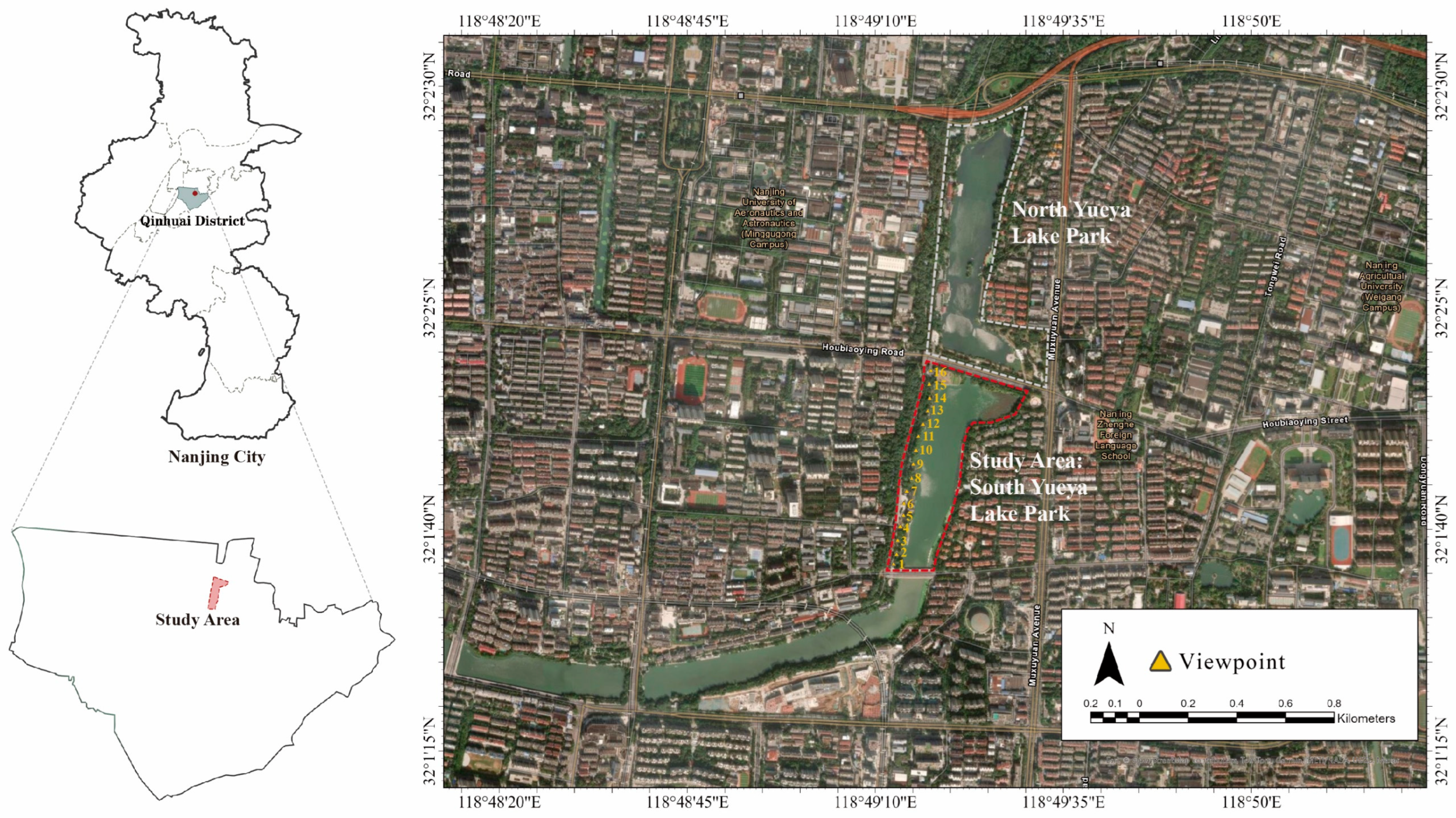
Figure 1. Study area and viewpoint distribution.
Land 14 02095 g001
Figure 2. The composition of the hybrid model.
Land 14 02095 g002
Figure 3. The main steps of the hybrid-model-based visibility analysis: (a) human vision simulation with Line of Sight (LoS)rays; (b) LoS analysis in ArcGIS Pro; (c) voxel-based LoS ray analysis.
Land 14 02095 g003
Figure 4. The value of visual exposure indicators and the average visual distance of all elements in the solid model (a) and the hybrid model (b).
Land 14 02095 g004
Figure 5. Visualization of typical views from selected viewpoints characterized by distinctive visual exposure indicators, shown for both the solid model and the hybrid model. The visualization of the solid model of (a1) viewpoint 2, (b1) viewpoint 6, (c1) viewpoint 10, (d1) viewpoint 13, (e1) viewpoint 14, and (f1) viewpoint 16; and the visualization of the hybrid model of (a2) viewpoint 2, (b2) viewpoint 6, (c2) viewpoint 10, (d2) viewpoint 13, (e2) viewpoint 14 and (f2) viewpoint 16.
Land 14 02095 g005
Table 1. Definitions and calculation methods for four visual exposure indicators.
IndicatorAbbreviationDefinitionCalculation Method
Green View Factor
[16,37,38]
GVFProportion of green vegetation visible from the pedestrian viewpoint G V F = N G r e e n N t o t a l × 100 %
Sky View Factor
[19,24,39]
SVFProportion of sky visible in the view from the pedestrian viewpoint S V F = N i n t e r v i s i N t o t a l × 100 %
Water View Factor
[13,20,40]
WVFProportion of large water surfaces (lakes, ponds, rivers) visible within the pedestrian’s field of view W V F = N W a t e r N t o t a l × 100 %
Building View Factor
[41]
BVFProportion of built structures visible within the field of view B V F = N B u i l d i n g N t o t a l × 100 %
Ground View FactorGRDVFProportion of ground surface visible within the pedestrian field of view G R D V F = N G r o u n d N t o t a l × 100 %
Table 2. Statistics of visual exposure indicators of the solid model and hybrid model.
View-PointGVI (%)SVF (%)WVF (%)BVF (%)GRDVF (%)
SHH-SSHH-SSHH-SSHH-SSHH-S
1041.5941.5949.7621.10−28.664.013.63−0.3815.701.09−14.6130.5332.592.06
2051.9851.9851.4219.89−31.536.324.04−2.2817.270.21−17.0624.9923.88−1.11
3043.3043.3049.5017.68−31.825.765.17−0.5920.190.15−20.0424.5533.709.15
4031.2031.2054.4032.11−22.295.704.72−0.9812.071.24−10.8327.8330.732.90
5029.6329.6346.4330.14−16.293.933.72−0.2123.232.69−20.5426.4133.827.41
606.386.3842.6238.93−3.692.072.070.0028.697.02−21.6726.6245.6018.98
7025.8925.8948.2935.01−13.283.012.86−0.1524.297.17−17.1224.4129.074.66
8055.0555.0552.7715.23−37.5410.339.77−0.5614.490.80−13.6922.4119.15−3.26
9049.2049.2052.1017.06−35.0411.5111.19−0.3215.140.97−14.1721.2521.580.33
10043.1843.1850.8017.98−32.8212.4612.22−0.2415.521.89−13.6321.2224.733.51
11057.9157.9148.977.94−41.0310.069.47−0.5917.941.65−16.2923.0323.030.00
12061.2861.2851.806.70−45.109.429.24−0.1815.230.59−14.6423.5522.19−1.36
13074.6874.6853.283.10−50.1810.667.08−3.5812.950.27−12.6823.1114.87−8.24
14037.1937.1952.8630.61−22.259.808.65−1.1514.141.27−12.8723.2022.28−0.92
15049.8549.8546.4914.55−31.943.573.13−0.4419.800.50−19.3030.1431.971.83
16026.9826.9851.5337.87−13.661.561.24−0.3215.204.10−11.1031.7129.81−1.90
Mean042.8342.8350.1921.62−28.576.896.14−0.7517.621.98−15.6425.3127.442.13
SD = Standard
Deviation
00.1660.1660.0310.1130.1260.0370.0350.0090.0450.0220.0340.0330.0740.061
Note: S = solid model, H = hybrid model.
Table 3. The statistics of visual distance (m) of all elements (except sky) in the solid model and hybrid model and their differences.
Landscape ElementsVegetationWater BodyBuildingGround
ViewpointSHH-SSHH-SSHH-SSHH-S
109.1439.143108.067102.416−5.65092.00353.772−38.23119.50711.636−7.870
207.7657.76582.84962.269−20.58090.85542.709−48.14721.5437.599−13.944
308.1548.15481.55775.297−6.26074.99834.901−40.09719.2406.989−12.251
4014.13914.13981.60168.414−13.187115.92559.500−56.42521.09911.753−9.347
5013.90813.90867.08560.115−6.97050.40036.809−13.59116.3758.472−7.903
6036.32836.32875.36575.128−0.23641.78332.326−9.45712.1017.885−4.216
7014.09914.09989.16084.039−5.12164.64454.881−9.76320.03412.237−7.797
8013.56913.56963.35260.045−3.307105.436150.09844.66224.24111.944−12.298
9011.68711.68758.51757.359−1.157111.028193.95682.92926.30618.046−8.260
10015.41015.41054.52953.956−0.57398.290158.58760.29725.36920.014−5.355
1108.3328.33260.72359.480−1.24389.332186.01596.68324.58920.818−3.771
1209.9019.90162.80461.272−1.532114.454154.58340.13024.43112.534−11.897
1305.3725.37259.59744.637−14.961134.556253.105118.55025.8378.982−16.855
14012.44712.44762.65555.225−7.430122.439141.43618.99727.28911.263−16.027
15012.14312.14399.42991.567−7.86278.09936.958−41.14125.0849.280−15.804
16011.80411.804141.639136.563−5.07793.65027.673−65.97726.18511.475−14.711
Mean012.76312.76378.05871.736−6.32292.368101.0828.71422.45211.933−10.519
SD = Standard
Deviation
06.8916.89123.03822.9125.69925.67573.66558.6814.1824.2444.285
Note: S = solid model, H = hybrid model.
Disclaimer/Publisher’s Note: The statements, opinions and data contained in all publications are solely those of the individual author(s) and contributor(s) and not of MDPI and/or the editor(s). MDPI and/or the editor(s) disclaim responsibility for any injury to people or property resulting from any ideas, methods, instructions or products referred to in the content.