Abstract
To understand how landscapes have changed in Yanqing District, Beijing, during its urban development over the past 15 years, we referred to the Landscape Character Assessment (LCA) theory, selecting altitude, slope, roughness, forest type, land cover, and forest vegetation cover as characteristic factors, identified nine types of landscape character types (LCTs) from 2005 to 2020 through unsupervised clustering. Then, we applied multi-model interpreters, including the Optimal Parameter-Based Geographical Detector (OPGD) and SHapley Additive exPlanations (SHAP), to analyze how social and natural factors impact the spatiotemporal changes of these LCTs. The results indicate that over the past 15 years, the landscape character of Yanqing District has undergone significant changes, with more frequent changes occurring in the “piedmont” areas where mountains meet plains. Slope and precipitation are the main factors affecting the intensity of LCT changes. In contrast, the transformation of different landscape characters is affected by factors such as altitude, slope, precipitation, and distance to artificial surfaces. This study reveals the dynamic changes in landscape character and their driving mechanisms, helping to develop more targeted strategies for landscape management in Yanqing District to promote sustainable regional development.
1. Introduction
Landscapes reflect the dynamic interaction between human actions and nature, embodying ecological value and defining the distinctiveness of various regions [1,2]. Yet, landscapes are ever-changing; as cities develop, diverse landscape types evolve through both human intervention and natural processes, reshaping the urban scenery [3]. Thus, understanding the dynamic changes of the entire landscape is crucial for setting tailored planning policies, devising protection and utilization strategies for the region’s landscape space, and managing its rational changes, ensuring the long-term sustainability of the regional landscape.
Most current studies on landscape evolution over time and space use land cover types, such as arable land, forest land, etc. [4,5,6]. Quantitative methods are often applied to describe this dynamic process, such as quantifying changes in the Landscape Pattern Index, the Land Use Change Index [7,8], or employing CA cellular automata models to predict future landscape evolution trends [9,10,11]. Therefore, some scholars have pointed out that from a landscape taxonomy perspective, existing studies often generalize landscapes based on land cover rather than specific representations [12,13]. For instance, sparse forests in plains and dense forests in mountainous areas exhibit distinctly different characters within forest landscapes classified as forest land. The transition from secondary planted forest to natural primary forest is often ignored since they are uniformly regarded as forest land. Therefore, a more precise method is needed to identify and categorize different environmental characters [13,14,15], implement assessment results, and propose corresponding management strategies.
Landscape Character Assessment (LCA) can divide landscape heterogeneity to compensate for the inadequacies in the description of land type representation. By comprehensively considering natural and cultural factors, objective and subjective factors, the unique characters of the landscape are classified and evaluated through a neutral value perspective, requiring that the characters must be factors that reflect the uniqueness of the landscape and evoke a specific sense of place [16,17]. Therefore, compared to traditional classifications in land type information, landscape character types (LCTs) more accurately represent a unique, identifiable, and unified pattern of landscape element assemblages [18,19,20]. The traditional LCA process consists of two main stages: 1. character classification and description; 2. character assessment and developing strategies. In the first stage, researchers use typological methods to define complex, multidimensional landscape boundaries in dynamic environments. This area has three main research approaches: (1) The intuitive classification method, in which, using databases from GIS or literature surveys, scholars classify landscape types based on visual description or subjective perception, integrating multiple attributes such as landscape visual aesthetics [21], historical context [22,23], soil type [24], and habitat morphology [25], etc. This method often appears in early landscape character studies. (2) The composite overlay method involves selecting specific variables to construct a classification framework and then applying mathematical methods for classification by composite overlay [26,27]. This method allows for a relatively reliable integration with multiple perception and natural physics dimensions. (3) The clustering method, similar to composite overlay, emphasizes the interconnection between landscape character description variables. It automatically identifies units with similar environments through clustering analysis [28,29,30], objectively describing the common “tendency” within a particular region. In the second stage, assessment can detach from traditional administrative regional boundaries, using heterogeneous landscape character as the basis for classification grouping, and evaluate landscape characters across various perspectives, for example, development guidance [31,32], landscape preferences [20,33], perception [34], landscape value exploration [35], etc. These evaluations lead to discussions on optimizing or preserving specific landscapes, guiding future management and conservation strategies.
However, only a few current LCA research studies use model tools that could incorporate dynamic changes into the analysis, such as analyzing seasonal, annual, or longer time scale variations. Therefore, based on the background mentioned above, the representation of landscape characters by land use is not sufficiently precise, and traditional LCA lacks dynamic assessment. We aim to develop an integrated method to accurately identify different types of landscapes and quantify their dynamic change patterns. We also explore the driving mechanisms of natural elements and human activities on landscape changes to provide more targeted strategies for landscape management. To fill these research gaps, this study selected Yanqing District in Beijing as a case example, mainly focusing on the following three key issues: (1) How has the landscape character in the study area evolved over the past fifteen years? (2) Which driving factors affect the changes in LCTs, and what scale makes this impact maximized? (3) Do various factors affect the transformation between LCTs differently? Under what circumstances is this transformation more likely to occur? We applied unsupervised two-step clustering methods to obtain the 2005–2020 long-term landscape characters. Then, the intervention of social and natural dimensions on LCTs’ spatial–temporal changes was explored using the Optimal Parameter-Based Geographical Detector (OPGD) and SHapley Additive exPlanation (SHAP) methods. The impact of various factors on landscape change was determined through explanatory Q values, mean SHAP values, and other metrics (Figure 1).
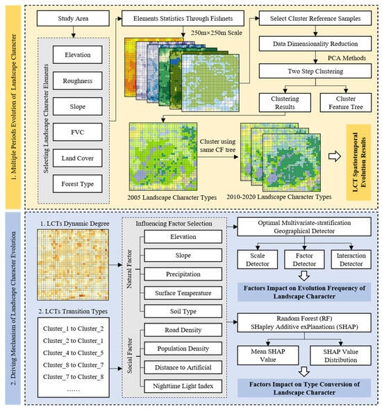
Figure 1.
Research flow of the current study.
The study selected Yanqing District in Beijing as the research area because this area represents an interwoven distribution of diverse landscapes. Over the last twenty years, landscape types have been consistently modified due to the influence of natural elements and human activities. Afforestation efforts in 2012 and 2017 have added 80,000 mu of artificial plantation forests. Significant land near the core of Yanqing’s urban area has been developed for infrastructure uses. Wetland and grassland areas have expanded due to the Guanting reservoir management projects. This study aligns with the planning goals of Yanqing District as a demonstration area for ecological civilization construction in Beijing, shifting from a singular “green space” perspective to consider the entire region as a diverse landscape. Then, looking for a generalizable theoretical approach to explain landscape changes, it provides a theoretical basis for comprehensive landscape management and protection decisions.
2. Materials and Methods
2.1. Research Area
Yanqing District (115°44′–116°34′ E, 40°16′–40°47′ N) is located in the northwest of Beijing (Figure 2), at the junction of the North China Plain and the Inner Mongolia Plateau, covering a total area of 1993.75 square kilometers and divided into 11 town-level administrative units. The region is surrounded by mountains on the east, south, and north sides, with rugged mountain terrain and a central depression forming an intermountain basin. With an average elevation above 500 m, resulting in a cool climate, it earns the title of Beijing’s “Summer Capital.” Yanqing District is an essential ecological conservation area in Beijing. Within the region, 12 nature reserves host around 1310 vegetation species. Due to successful afforestation and conservation projects in recent years, the forest coverage rate has reached 61.8%. However, there is a certain difference in the composition of vegetation communities between natural and planted forests. Natural forests mainly comprise Liaodong oak and Chinese pine, while planted forests primarily consist of poplar, willow, elm, locust, Chinese toon, and cypress. Over time, the secondary communities of planted forests gradually evolve towards natural forests.
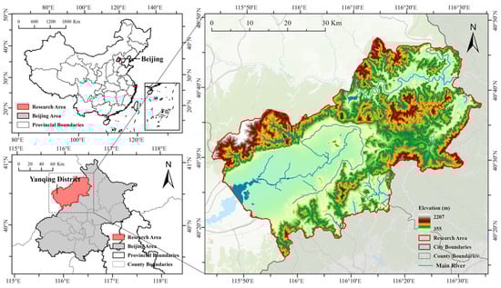
Figure 2.
Study area.
2.2. Data and Pre-Precession
The data in this study were primarily applied in two aspects: the landscape character description and the driving factors of landscape character changes.
For landscape character description, in addition to widely used factors such as elevation [36,37], slope [38], roughness [39], and land cover [27,40,41], the study also considered forest types and vegetation coverage as description elements. Natural forests are often perceived as more diverse ecosystems, whereas planted forests may leave a strong impression of human intervention due to their neatness and uniformity [42]. Studies also indicate that forest types affect the region’s ecological soundscape (such as bird songs), subsequently influencing psychological recovery and relaxation [43]. Vegetation cover directly impacts the visual openness and screening effect of the landscape. High vegetation cover may provide psychological privacy and low mental pressure [44], while low cover offers a more open landscape view. Therefore, a characteristic description system comprising six factors was selected to comprehensively describe the landscape from physical characteristics and perception (Figure 3). Elevation, slope, and roughness data were derived from the ASTER GDEM V3 dataset (https://urs.earthdata.nasa.gov, accessed on 17 March 2025), processed in ArcGIS Pro 3.3. Land use data were derived from the GLC_FCS30D dataset by the Aerospace Information Research Institute of the Chinese Academy of Sciences [45], using the primary land cover classification of this dataset, dividing the study area into eight categories: cropland, forest, shrubland, grassland, wetland, impervious surface, bare areas, and water. Fractional vegetation cover (FVC) data were sourced from the monthly average FVC data of the National Tibetan Plateau Data Center, using the monthly maximum value to synthesize annual average FVC data [46]. Forest type data were derived from the global forest management type dataset obtained by Xu et al. [47]. Through machine learning, the forest types within the study area were divided into four categories, naturally forest, planted forest, agroforestry, and others, according to the needs of landscape character research.
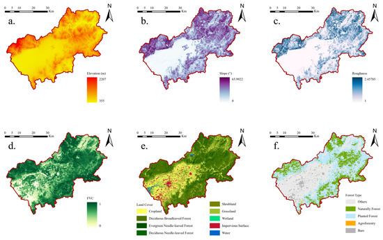
Figure 3.
Landscape character description factors: (a) elevation; (b) slope; (c) roughness; (d) fvc; (e) land cover; (f) forest type.
For driving factors of landscape character changes, the research considered the impact of landscape character changes from both natural and social aspects, selecting nine influencing factors. Natural factors include elevation, slope, precipitation, surface temperature, and soil type, which are primarily used to describe the natural environment required for surrounding topography and vegetation growth. For example, temperature may affect the rate of vegetation transpiration, and the soil’s physical and chemical properties may determine vegetation types and distribution patterns. Social factors include road density, distance to artificial area, population density, and nighttime light index, which mainly reflect the impact of human distribution and construction activities on landscape characteristics. Road density indicates the region’s traffic accessibility, the distance to artificial areas can suggest the potential disturbance of human activities on natural landscapes [4], and population density and nighttime light index are used to measure population distribution and economic activity intensity [48]. Data sources are detailed in Table 1. Elevation, slope, and soil type use single-period data identical to the source data as driving factors. We selected the source data from the initial and final time points for other data types to calculate the average. For instance, for the period from 2005 to 2010, we averaged the data from 2005 and 2010. Subsequently, all data were analyzed within different unit areas using ArcGIS Pro 3.3, such as 1000 m, 2000 m, and 3000 m grids. Road density is line density, calculated as the total length of all roads within a unit area. Soil type is a categorical variable calculated as a constant. This study used the OLS model for collinearity detection, with the maximum Variance Inflation Factor (VIF) being 5.814, which is less than 10, indicating passing the collinearity test. For convenience in subsequent research, all study factors are named X1–X9.

Table 1.
Driving factors data details.
2.3. Multi-Period LCTs Identification
The study applied a clustering method using six factors to assess the landscape character of Yanqing District. First, defining the unit pixel as the foundational unit for classification is necessary. To balance scale and statistical needs (such as calculating averages), a 250 m scale was selected for the optimal landscape character unit. Using ArcGIS’s fishnet tool, Yanqing District was divided into 31,631 units. Through the table summary function, the average values of four types of continuous data—elevation, slope, roughness, and FVC—within the 0.25 km × 0.25 km unit area were calculated, along with the constant values for two categorical data types—forest type and land use—to form the basic database.
In this database, elevation, slope, and roughness describe geomorphological character. To prevent these factors from disproportionately influencing the clustering analysis, the study imported these three factors into SPSS 26.0 for dimensionality reduction through principal component analysis (Table A1). Consequently, Principal Component 1 was chosen to represent the three geomorphological factors and was incorporated into the clustering analysis.
This study utilized the two-step clustering method, which is advantageous as it can calculate both continuous and categorical data. It uses the BIRCH algorithm’s clustering feature tree (CF tree) to record cluster centroids and diameters, allowing data with high similarity to be classified within the same tree node. By constructing a CF classification feature tree for landscape character, approximate clustering results for different data groups over multiple years can be achieved, avoiding issues such as cluster centroid shift. The study used a two-step clustering algorithm, prioritizing clustering with the 2005 data as the sample. Parameters were set using the log-likelihood distance and the Bayesian criterion.
The silhouette coefficient Equation (1) determines the optimal number of clusters. The silhouette coefficient quantifies the degree of dispersion between the clusters [50]. represents the average silhouette coefficient for the clustering, represents the silhouette coefficient for the sample point , represents the average distance between the sample point and all other points in the same cluster, and represents the average distance between the sample point and all points in the nearest different cluster.
Results show that the silhouette coefficient reaches a maximum value of 0.616 with nine clusters, indicating the best cohesion and separation among clusters. A CF tree was constructed with nine classified clusters and applied to the remaining three datasets from 2010, 2015, and 2020, ultimately obtaining the landscape character classification results for Yanqing District across four periods (Figure 4).
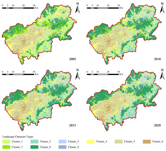
Figure 4.
Spatial distribution of LCTs in 2005, 2010, 2015, and 2020.
2.4. Spatiotemporal Changes Analysis
To effectively assess the intensity and type of spatial–temporal changes, this study employed two main indicators for describing LCTs’ changes: LCT dynamic degree () and LCT transition types. LCT dynamic degree () refers to the calculation method of land use dynamic degree [51], with the formula Equation (2) as follows:
Here, represents the total area of the unit region, represents the absolute total value of the area transformed between the i-th landscape character type and other landscape character types j, is the number of landscape character types, and represents the interval of the study period, increasing by 1 every 5 years. reflects the intensity of landscape character type changes in the corresponding unit region during this period.
Each 250 m landscape character grid serves as a sample for LCTs transition types, recording whether a transition from landscape type i to landscape type j occurred from 2005 to 2020. “Yes” is assigned a value of 1, “No” is assigned a value of 0, and transitions are labeled as “Cluster_n to Cluster_m,” where n represents the initial landscape character type and m represents the changed landscape character type.
2.5. Optimal Parameter-Based Geographical Detector (OPGD)
The Optimal Parameter-Based Geographical Detector (OPGD) is a tool for exploring spatial heterogeneity, identifying the interactive effects of geographical factors, and assessing risks. This tool calculates the explanatory quantity and significance P to reflect whether different elements have associated impacts in space. As an improved model, OPGD employs various methods to discretize continuous data, including natural breaks, equal breaks, geometric breaks, quantile breaks, and standard deviation breaks, to obtain the most significant value within a set range of intervals [52]. Additionally, OPGD allows exploration of changes in values across different spatial scales. In this study, the spatial scale comparison, factor detector and interaction detector of OPGD were used to analyze how the explanatory quantity of driving factors on the LCT dynamic degree () changes across different spatial scales, and whether the interaction between factors enhances or diminishes . The calculation method for values is determined using Equation (3):
Here, denotes the explanatory power of a specific driving factor, with a range between [0, 1]; refers to the stratification of the driving factor; and represent the total number of samples and the number within stratification , respectively; and are the variance of the entire region and the variance within stratification .
The study used the nine previously mentioned elements (X1–X9) as driving factors (Table 1). Starting with a grid size of 500 m, each subsequent 500 m interval is defined as a spatial scale unit, with the driving factors serving as independent variables X and the LCTs dynamic degree () as the dependent variable Y, continuing until the 6000 m grid ends the statistics. The “GD” package in R was employed to run the Optimal Parameter-Based Geographical Detector model, analyzing spatial heterogeneity and driving mechanisms.
2.6. SHapley Additive exPlanations (SHAP)
To further explore the impact of elements from both natural and social dimensions on landscape character transformation, the study utilized an interpretable machine learning model based on Random Forest (RF) [53] and SHapley Additive exPlanations (SHAP) [54] in Python 3.10. RF employed a binary classification model, using nine driving factors as independent variables, with LCT transition types considered predictive variables. A transformation from “Cluster_n to Cluster_m” was assigned a value of 1; otherwise, it was 0. 80% of the feature transformation sample data was used as the training set to build the model, with the remaining 20% considered the validation set to evaluate the model. Subsequently, SHAP was applied to interpret the machine learning results. Based on the Shapley value principle from game theory, SHAP effectively elucidates the significance of feature values during prediction. The contribution of driving factors to various landscape character transformations can be determined by comparing average SHAP values. Furthermore, by comparing the different SHAP distributions caused by varying values of the driving factors, the study can explain how these factors promote or inhibit changes in LCTs. The formula for calculating SHAP values is as follows:
In Equation (4), is the SHAP value of factor , indicating the magnitude of the factor’s impact on accessibility; is the factors’ subset used in the model; is the vector of sample factor feature values to be explained; is the number of factors; represents the weight, and refers to the model output value under the factor combination .
3. Results
3.1. Results of Landscape Character Identification
Using CF clustering trees on data from 2005 to 2020, the study obtained 9 types of clustering results with similar characteristics in Yanqing District across 4 periods. These are named from cluster_1 to cluster_9. After receiving the results, we merged and statistically analyzed the clustering data, conducted field surveys for verification, and took representative photos. The characteristics of each type are shown in Table 2.
Table 2.
Landscape character description.
Clusters 1 to 6 feature lower altitudes (average below 700 m), while clusters 7, 8, and 9 are high-altitude landscapes. Cluster_1 and Cluster_2 both represent low-altitude mountain forest landscapes, but the former consists of artificially planted broadleaf forests distributed in suburban valleys and around roads; the latter comprises naturally broadleaf forests that have undergone secondary succession, along with some agroforestry, located in shallow mountain areas untouched by human activities. Cluster_3 is characterized by mixed forest and grassland mountain areas where deciduous and broadleaf trees coexist. These areas have relatively poor soil, leading to slow tree growth but thriving herbaceous plants. Cluster_4 includes flat wetland and plain grassland landscapes with low vegetation coverage (average 0.47), but for different reasons. Wetland landscapes have low coverage due to water influence, with rich plant diversity and scenic beauty around the Yongding River system on the region’s west side. Plain grasslands near the lower mountains show soil exposure due to farming and construction. Cluster_5 and Cluster_6 represent plain farmland landscapes and urban landscapes primarily created by human activities. These two landscapes occupy large central areas of Yanqing District and are interspersed with each other, with few wild plants besides crops. Cluster_7 and Cluster_8 are higher altitude mountain forest landscapes, similar to Cluster_1 and Cluster_2, but at higher altitudes with rugged terrain, minimal human activity, and better vegetation growth. Cluster_9 represents Yanqing District’s high-altitude artificial and natural mixed forest-grassland zone, characterized by a cold and dry climate, ideal for herbaceous plant growth. A rich herbaceous community forms beneath artificially planted forests, gradually transitioning to a natural landscape.
Figure 5 illustrates the area statistics for various landscape characters from 2005 to 2020. The deciduous broadleaf artificial forests represented by Cluster_1 and Cluster_7 experienced a notable reduction in area over 15 years, with Cluster_1 decreasing by 190.04 square kilometers and Cluster_7 by 198.18 square kilometers. In contrast, the low-altitude deciduous broadleaf forest mountain landscape (Cluster_2), which expanded by 190.23 square kilometers, and the mid-altitude deciduous broadleaf forest mountain landscape (Cluster_8), which expanded by 198.61 square kilometers. Cluster_3 increased by 64.23 square kilometers over 15 years but showed instability, indicating increased natural forest-grass mixed zones in shallow mountain areas. The low-altitude wetland-grass mixed plain landscape represented by Cluster_4 decreased in quantity. The urban landscape cluster_6 slightly increased by 10.72 square kilometers.
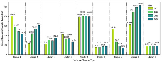
Figure 5.
Area statistics for various LCTs in 2005, 2010, 2015, and 2020.
3.2. Results of LCT Dynamic Degree and Type Transition
Figure 6 illustrates the LCT dynamic degree () of landscape character using a 500 m observation scale. Over the four periods, the regions where landscape character transitions occurred more frequently were roughly the same, indicating that the mountainous areas near the Yanqing region’s boundary are more prone to frequent landscape character transitions. Among these, the period from 2005 to 2010 saw the most intense changes, especially in the transitional zones between the central plains and mountains, where many areas underwent complete landscape type transitions ( =1). From 2010 to 2015, landscape character transition began to slow, particularly in the mid-northern mountainous landscapes of the Yanqing Baili Gallery Scenic Area, which started stabilizing. From 2015 to 2020, changes in landscape character further decreased, mainly concentrated in suburban mountainous areas near urban regions, with higher altitude landscapes experiencing little change. Overall, from 2000 to 2020, landscape character changes in mountainous areas far from urban centers occurred much faster than in areas closer to city centers, with slight variation in change rates among mountainous areas, indicating widespread transformation.
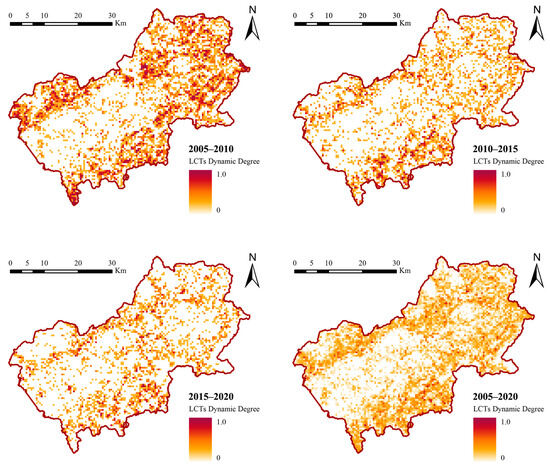
Figure 6.
LCT dynamic degree across different periods.
The study employed proportional chord diagrams to illustrate landscape characters’ transition types and areas across four periods (Figure 7). From 2005 to 2010, the most common transition was from Cluster_7 to Cluster_8, transitioning from mid-altitude artificial deciduous broadleaf forest mountain landscape to mid-altitude natural deciduous broadleaf forest mountain landscape, covering 151.90 square kilometers. From 2010 to 2015, the predominant transition was from low-altitude artificial deciduous broadleaf forest mountain landscape to low-altitude natural deciduous broadleaf forest mountain landscape (Cluster_1 to Cluster_2), with 75.32 square kilometers changing. The trend from 2015 to 2020 mirrored that of 2010 to 2015, with most transitions occurring in low-altitude regions. Over the entire period from 2005 to 2020, the mid-altitude forest-grass mixed mountain landscape (Cluster_9) was the most stable landscape type, with no significant type transitions. Additionally, Forest landscapes were more prone to type transitions.
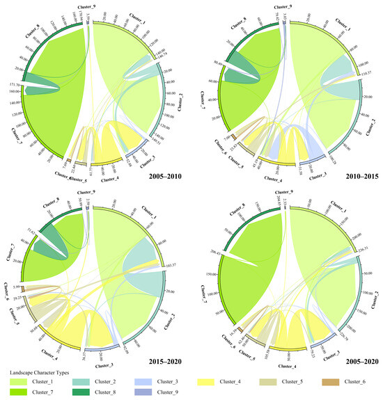
Figure 7.
LCTs type transition across different periods.
3.3. Driving Mechanism of LCTs Dynamic Degree by OPGD
3.3.1. Impact of Spatial Scale
In the statistical analysis of geographical elements, spatial aggregation calculated with different partition sizes and shapes can exhibit varying spatial patterns, distribution relationships, or statistical correlations, indicating the presence of spatial scale effects [55]. Thus, the study initially calculated the changes in single-factor Q values and the 90th percentile for nine natural and social factors at different scales using a 500 m interval to identify the optimal spatial scale division (Figure 8). The results show that the explanatory power Q of various driving factors for the dynamic degree of LCTs in four periods increases unstably with scale, but shows a significant decrease in significance. Most factors’ impact on the dynamic degree becomes insignificant beyond 4500 m. Consequently, the study chose 4500 m as the optimal spatial scale, and all subsequent OPGD detection results are based on this scale.
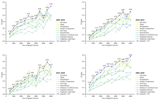
Figure 8.
Variation of Q values across different scales. Purple indicates the 90th percentile, and the light gray represents scales with insignificant explanatory power (p > 0.05).
3.3.2. Impact of Single Factors
Based on the results from OPGD’s single-factor detector (Table 3), slope (X2) was the primary driving factor for LCT dynamics from 2005 to 2010, with an explanatory power Q value of 0.502, followed by distance to artificial area (X7). The trends for 2010–2015 and 2015–2020 are roughly the same, with precipitation (X3) being the primary factor driving landscape character changes. For the overall LCTs dynamic degree from 2005 to 2020, slope (X2) has the most significant impact, with an explanatory power Q value of 0.53. Generally, factors closely related to the intensity of landscape character changes include elevation (X1), slope (X2), precipitation (X3), road density (X6), and population density (X8). Table A2 provides detailed information on the discretization method and number.
Table 3.
Explanatory Q values for driving factors across different periods.
3.3.3. Impact of Factor Interactions
According to the results from OPGD’s interaction detector (Figure 9), the intensity of landscape character changes is influenced by interactions between different driving factors, resulting in either double-factor enhancement or nonlinear enhancement, with the former being more common. This indicates that compared to independent single factors, the interaction of multiple factors increases the explanatory power for the LCT dynamic degree. Notably, the Nighttime Light Index (X9) generally exhibited higher Q values through interactions with other factors. From 2005 to 2010, the combination of elevation (X1) and distance to artificial area (X7) was the primary reason for landscape character transformation, with a Q value reaching 0.682. From 2010 to 2015 and 2015 to 2020, the combination of slope (X2) and Nighttime Light Index (X9) provided the strongest explanation for landscape character dynamics. Overall, from 2005 to 2020, the pairwise combinations of Nighttime Light Index (X9) with elevation (X1) and slope (X2) had the strongest explanatory power (Q = 0.699). Additionally, the study found that the combined effect of natural factors (X1, X2, X3, X4, and X5) and social factors (X6, X7, X8, and X9) offers higher explanatory power than combinations of only natural or social factors, suggesting that both natural conditions and human activities more likely influence landscape character changes.
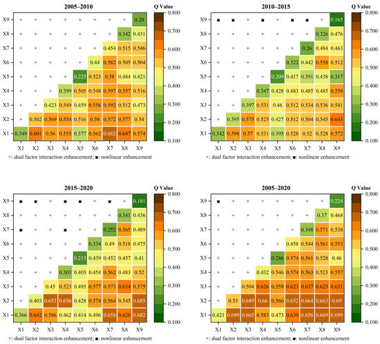
Figure 9.
Interaction types and explanatory Q values of driving factors’ interaction.
3.4. Driving Mechanism of Landscape Character Type Transition by SHAP
3.4.1. Overall Importance of Driving Factors
The study used average SHAP values to assess the contribution of driving factors to the various landscape character type transitions. As illustrated in the results (Figure 10), the radial bar values indicate the overall importance of driving factors X1-X9 for type transitions, with larger values signifying greater importance. Elevation (X1) is the primary reason for the transitions of Cluster_1 to Cluster_2, Cluster_2 to Cluster_1, Cluster_7 to Cluster_8, and Cluster_8 to Cluster_7, indicating that elevation is the main factor driving the mutual transformation between artificial and natural deciduous broadleaf forest landscapes. Slope (X2) primarily influences the transitions between Cluster_4 and Cluster_5, and Cluster_5 and Cluster_4, reflecting the conversion between wetland–grass mixed landscapes and farmland landscapes. Surface temperature (X4) contributes most significantly to the transitions between Cluster_3 and Cluster_4, and Cluster_4 and Cluster_3, suggesting that surface temperature is more likely to lead to conversions between wetland–grass mixed landscape and forest–grass mixed landscape. Distance to artificial area (X7) has the highest explanatory value of 0.213 for the transition from Cluster_5 to Cluster_6, indicating that locations closer to urban centers are more likely to see farmland converted into metropolitan areas.
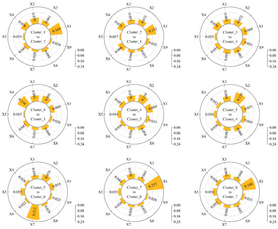
Figure 10.
Mean SHAP values of driving factors for different transition types.
3.4.2. Influence Direction on Character Type Transition
Bee swarm plots can illustrate the direction of influence of identified driving factors on landscape character transitions and whether a linear relationship exists (Figure 11). The results show that in the mutual transformation between Cluster_1 and Cluster_2, elevation (X1) and surface temperature (X4) exhibit a noticeable inhibitory effect, while higher precipitation (X3) and slope (X2) facilitate the transitions. In the mutual transformation between Cluster_3 and Cluster_4, high surface temperature (X4) and high Nighttime Light Index (X9) promote transitions, whereas precipitation (X3) and elevation (X1) have inhibitory effects. Additionally, a greater distance from the artificial area favors transitions from Cluster_4 to Cluster_3. In the mutual transformation between Cluster_4 and Cluster_5, higher slope (X2) and precipitation (X3) values make landscape transitions less likely. At the same time, road density (X6) and soil type, such as brown soil (derived from categorical number), show slight promotion, with other insignificant factors. Areas closer to artificial areas, with gentle slopes, lower population density, and brown soil, are more prone to transitioning from Cluster_5 to Cluster_6. In the mutual transformation between Cluster_7 and Cluster_8, elevation (X1), slope (X2), and precipitation (X3) significantly promote landscape type transitions, while surface temperature (X4) shows an inhibitory effect. Distance to artificial area (X7) also facilitates transitions between these landscape types, though the effect is less pronounced.
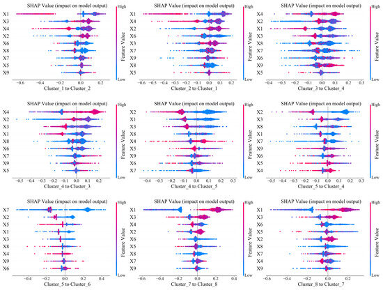
Figure 11.
Shapley value contributions (Bee Swarm) of driving factors. The Y-axis of the figure is arranged in descending order of global importance (mean SHAP value) from top to bottom.
4. Discussion
4.1. The Advantages of Landscape Characters Relative to Traditional Land Use
Unique landscapes combine natural beauty, cultural significance, and ecological importance, creating distinct value. For example, coniferous and broadleaf mixed forests and rocky streamside landscapes can significantly alleviate stress and depression, maintaining mental health [56]; wetland types with moderate vegetation coverage may have the highest bird richness and support bird migration [57]; the litter content in natural secondary forests is significantly higher than in artificial forests, providing more material for soil carbon sequestration and improving soil quality [58]. Meanwhile, landscapes are inherently dynamic, and understanding how to effectively preserve and incorporate valuable elements and areas within modern urbanized and globalized society is crucial [59]. In existing dynamic studies, most research is based on changes in land use to explain changes in landscape character, perception, and pattern [60,61,62]. However, the complexity and diversity of landscapes result from the combined effects of various natural and human factors, not just direct explanations from land use [59,63,64]. Therefore, this paper suggests using Landscape Character Assessment (LCA) methods to finely subdivide landscapes to distinguish different landscape character areas and assess multidimensional value potential, thereby aiding the formulation of urban planning policies. However, current research on landscape character mainly focuses on the subdivision and assessment of the current environment [31,33,35]. Due to landscapes’ fluid and ever-changing nature, any strict landscape character classification scheme will become outdated [65]. This study employs a CF classification tree-based two-step clustering to understand this change process and identify nine representative landscape character types from 2005 to 2020. For example, Cluster_4 represents a low-altitude flat medium-coverage wetland–grass mixed plain landscape, while Cluster_8 represents a mid-altitude rugged high-coverage natural deciduous broadleaf forest mountain landscape. This clustering method, integrating multiple indicator systems such as elevation, slope, roughness, FVC, land cover, and forest type, can eliminate subjective bias and objectively quantify specific landscape changes.
4.2. The Relationship Between Changes in Landscape Character and Multidimensional Factors
This study approaches the understanding of landscape character changes from two perspectives: dynamics and transformation types. OPGD and SHAP interpretable machine learning models based on Random Forest were used to analyze their relationship with various driving factors. The results indicate that the “intensity” and “type” of landscape character changes are driven by different factors, with dominant factors varying across periods and transformation types, suggesting that landscape dynamics are not solely influenced by a specific element but rather by the complex interplay of natural conditions and human activities [66,67,68].
According to OPGD analysis, the “intensity” of landscape character changes is generally dominated by natural factors, with slope and precipitation being the most relevant factors. Areas with high landscape dynamics in Yanqing District are typically concentrated in the “piedmont” area at the junction of mountains and plains. The steep slopes in the “piedmont” area increase soil erosion rates. At the same time, precipitation-induced water runoff further accelerates sediment migration [69,70], potentially affecting the vegetation growth environment, making landscapes more prone to change. The study also found that the interaction between social factors, represented by nighttime light index and distance to artificial area, and natural elements significantly enhances the explanatory power of change “intensity.” This result indirectly proves that landscape transformation is more likely due to the combined influence of natural conditions and human activities, mainly related to Yanqing District’s recent production construction and urban expansion. SHAP further explains the causes of transformation types. The study also found that the transformation from an artificial deciduous broadleaf forest landscape to a natural deciduous broadleaf forest landscape is mainly related to elevation [71,72], with extreme elevation values (either very low or very high) facilitating type conversion. Low slope and low precipitation wetland–grass mixed landscapes are more likely to convert into farmland plain landscapes, while distance to artificial area determines the conversion of farmland plain landscapes into urban landscapes, forming a continuous driving chain. This indirectly verifies that farmland reclamation chooses areas with lower erosion risk [73,74]. Higher surface temperature makes wetland–grass mixed landscapes more likely to convert into forest–grass mixed landscapes, possibly due to increased evaporation from wetlands caused by rising surface temperatures, accelerating wetland disappearance [75,76]. Additionally, the study found that under similar external environmental conditions, landscapes may tend to transform into a specific type, but there will still be repeated bidirectional “adaptive cycles” [77]. We have two possible hypotheses for this phenomenon: (1) a coupling relationship and threshold effect exists among multiple factors, and the factors themselves may also change, preventing stable landscape transformations. For instance, shifts from wetland–grassland to forest–grassland landscapes tend to occur in areas with higher surface temperatures and distances from artificial surfaces. Still, these elements do not necessarily change synchronously over time. Specifically, although high-temperature weather in Beijing has gradually increased in recent years, extensive waterway connectivity restoration projects have been implemented around the Guanting Reservoir near developed areas, enhancing its water retention capacity. Natural and social factors no longer constitute a synergistic relationship, leading to wetland landscapes that cyclically disappear and reappear. (2) Although areas share similar environmental conditions, hidden influences like natural disasters or socioeconomic activities could lead to cyclical landscape changes. Research indicates that afforestation practices with artificial forests could trigger recurrent changes [78]. In the past, Yanqing District had traditional activities like kiln firing and grazing. Natural forests shrank due to damage from logging, wildfires, and livestock farming, and were restored by afforestation efforts. They recovered into natural forests through secondary succession, forming a landscape cycle. In conclusion, landscape change is a dynamic, reversible, and cyclical process, inevitably influenced by a combination of complex conditions rather than a linear, unidirectional relationship.
4.3. Implications of Landscape Character Changes for Urban Management Policies
This study explores the changes in landscape characters in Yanqing District and their driving mechanisms. The findings may provide references for urban managers in two aspects when formulating future green space management policies: (1) They indicate potential risks in areas with frequent landscape transitions. LCT dynamic degree can quantitatively describe regions prone to frequent character transitions, where landscapes exhibit instability, suggesting that any construction activities affecting landscape appearance may pose risks. For instance, the “foothill” zones in Yanqing District face water and soil loss issues due to surface runoff and soil erosion. When formulating farmland reclamation policies for this area, a comprehensive assessment of the surrounding environment’s suitability should be conducted, and a series of water and soil conservation measures should be included in future development plans. (2) They enable the protection of special types of regional landscapes. Compared to land use, changes in special LCTs with regional characteristics can better reveal potential changes in urban ecosystem services such as ecological habitat quality and recreational services, thereby supporting urban-related landscape management policies. For example, the continuous reduction in natural forest–grassland wetlands over 15 years indicates the gradual degradation of wetland ecosystems during urban development. Future urban planners should be vigilant about habitat loss and weakened biodiversity. Moreover, protection areas for migratory birds and native aquatic fish should be clearly delineated. By detecting changes in landscape characters, reasonable planning of human–land relationships can be achieved, promoting sustainable development and ecological protection.
4.4. Limitations and Prospects
This study utilizes the Optimal Parameter-Based Geographical Detector (OPGD) and SHapley Additive exPlanation (SHAP) methods to quantitatively explain the impact of social and natural dimensions on landscape changes, revealing the intrinsic evolutionary logic of certain exceptional regional landscapes. Despite this, the study has some limitations and shortcomings. Landscape Character Assessment emphasizes the uniqueness of landscapes and their perception by humans [79], choosing among landscape character description factors that are particularly important. However, obtaining historical data for Yanqing District poses challenges due to long-term evolution. For example, canopy height data can be used to measure the role of plant height in influencing human vertical perception [80]. Nevertheless, with the recent proliferation of satellite sensors like ICESat-2, it is possible to collect and describe such characteristic factors. Additionally, the SHAP method used in this study is based on a single machine learning model, Random Forest, optimized with hyperparameters. Although Random Forest often exhibits superior performance in classification and regression tasks in the remote sensing field [81,82], the lack of comparison with other competitive models may prevent determining whether Random Forest is the optimal choice for binary classification problems in type conversion. Future research could include comparative studies of multiple machine learning models based on SHAP (SVM, XGboost, LightGBM, etc.) to further improve the accuracy and generality of the driving mechanism explanation model.
Looking forward, further assessment of the impacts and trends brought by dynamic landscape characters can aid urban development decision-making. Specifically, the research can be divided into two directions: (1) assessing changes in potential values such as landscape pattern, ecosystem service capacity, and tourism development potential brought by dynamic landscape character changes, and their possible impacts on urban development; (2) predicting future trends in landscape character changes, evaluating whether certain types of landscapes face risks of disappearance or fragmentation in the future, to avoid issues of landscape homogenization brought by urban development.
5. Conclusions
Yanqing District was chosen as the research site in this study, where an unsupervised two-step clustering method was applied. This method considered elevation, slope, relief, forest type, land use, and forest vegetation coverage to identify nine distinct landscape character types (LCTs) between 2005 and 2020. Additionally, Optimal Parameter-Based Geographical Detector (OPGD) and SHapley Additive exPlanation (SHAP) methods were used to analyze how social and natural factors influence these landscapes’ spatial and temporal changes. The main conclusions of this research are as follows:
(1) Low-altitude and mid-altitude artificial broadleaf forest landscapes significantly decreased by 190.04 square kilometers and 198.18 square kilometers, respectively, over 15 years. Natural broadleaf forest landscapes increased significantly, indicating a transition from artificial to natural forests. At the same time, the quantity of low-altitude wetland-grass mixed plain landscapes decreased, while plain farmland and urban landscapes slightly increased, showing the trend of land development expansion in Yanqing District in recent years.
(2) The period from 2005 to 2010 saw the most intense changes, especially in the “piedmont” areas at the junction of mountains and plains, where landscape changes were more frequent. Slope and precipitation are the main natural factors affecting the intensity of landscape dynamic changes, with the 4500 m area range being the most significant spatial scale for this impact. Additionally, the interaction between nighttime light index and distance to artificial areas with natural factors significantly enhanced the explanatory power for the intensity of landscape changes, indicating that the combined effects of human activities and natural conditions influence the changes of landscape characters.
(3) Elevation is the main factor in the mutual transformation between artificial and natural broadleaf forest landscapes. Extreme elevation values more easily facilitate type conversion. Slope and precipitation affect the conversion between wetland–grass mixed landscapes and farmland landscapes, while the distance to artificial areas determines the conversion of farmland landscapes to urban landscapes. Higher surface temperatures make wetland–grass mixed landscapes more likely to convert into forest–grass mixed landscapes.
The findings of this study contribute to the rational planning of regional human–land relationships and provide a scientific basis for regional green space management policies.
Author Contributions
Conceptualization, D.L. and X.C.; methodology, X.C.; software, D.L. and S.Z.; validation, J.Z. and S.T.; formal analysis, D.L.; investigation, J.L. and X.C.; resources, D.L.; data curation, D.L.; writing—original draft preparation, D.L.; writing—review and editing, J.Z. and S.T.; visualization, D.L., J.L. and S.Z.; supervision, X.C.; project administration, X.C.; funding acquisition, D.L. All authors have read and agreed to the published version of the manuscript.
Funding
This research was funded by the China Scholarship Council, grant number 202406510010.
Data Availability Statement
The raw data supporting the conclusions of this article will be made available by the authors upon request.
Conflicts of Interest
The authors declare no conflicts of interest. The funders had no role in the design of the study; in the collection, analyses, or interpretation of data; in the writing of the manuscript; or in the decision to publish the results.
Appendix A
Appendix A.1. Results of Principal Component Analysis
Table A1 revealed the variance explained and factor loading for three principal components. Principal Component 1 had a variance explanation rate of 82.273 and was highly correlated with elevation, roughness, and slope. Principal Component 2 only had a loading coefficient of 0.555 in elevation. Principal Component 3 did not show any high values in either the variance explanation rate or the loading coefficient.
Table A1.
Principal component indicators.
Table A1.
Principal component indicators.
| Principal Component | Total Variance Explained | Factor Loading | |||
|---|---|---|---|---|---|
| Eigen Value | Cumulative Var | Elevation | Roughness | Slope | |
| 1 | 2.468 | 82.273 | 0.831 | 0.924 | 0.962 |
| 2 | 0.444 | 97.079 | 0.555 | −0.334 | −0.158 |
| 3 | 0.088 | 100 | 0.05 | 0.188 | −0.223 |
Appendix A.2. Optimal Discretization Method and Number
Table A2 indicates that the most optimal classification intervals ranged from 6 to 9, with five classification methods: natural breaks, equal breaks, geometric breaks, quantile breaks, and standard deviation breaks.
Table A2.
Discretization method and number across different periods.
Table A2.
Discretization method and number across different periods.
| Factor | 2005–2010 | 2010–2015 | 2015–2020 | 2005–2020 | ||||
|---|---|---|---|---|---|---|---|---|
| X1 | Quantile | 8 | Quantile | 8 | Quantile | 7 | Quantile | 8 |
| X2 | Natural | 6 | Equal | 8 | Quantile | 9 | Equal | 8 |
| X3 | Equal | 8 | Natural | 9 | SD | 8 | Natural | 9 |
| X4 | Quantile | 6 | Quantile | 7 | SD | 8 | Geometric | 8 |
| X5 | — | — | — | — | — | — | — | — |
| X6 | Geometric | 7 | Quantile | 9 | Geometric | 9 | Geometric | 9 |
| X7 | Natural | 8 | Geometric | 9 | Quantile | 9 | Natural | 9 |
| X8 | Quantile | 6 | Quantile | 6 | Quantile | 9 | Quantile | 6 |
| X9 | Natural | 8 | Quantile | 8 | Quantile | 9 | Quantile | 9 |
“—” indicates categorical variables, which don’t require discretization.
References
- Bastian, O.; Grunewald, K.; Syrbe, R.-U.; Walz, U.; Wende, W. Landscape Services: The Concept and Its Practical Relevance. Landsc. Ecol. 2014, 29, 1463–1479. [Google Scholar] [CrossRef]
- Hersperger, A.M.; Grădinaru, S.R.; Pierri Daunt, A.B.; Imhof, C.S.; Fan, P. Landscape Ecological Concepts in Planning: Review of Recent Developments. Landsc. Ecol. 2021, 36, 2329–2345. [Google Scholar] [CrossRef] [PubMed]
- Bürgi, M.; Hersperger, A.M.; Schneeberger, N. Driving Forces of Landscape Change—Current and New Directions. Landsc. Ecol. 2005, 19, 857–868. [Google Scholar] [CrossRef]
- Seto, K.C.; Fragkias, M. Quantifying Spatiotemporal Patterns of Urban Land-Use Change in Four Cities of China with Time Series Landscape Metrics. Landsc. Ecol. 2005, 20, 871–888. [Google Scholar] [CrossRef]
- Deng, J.S.; Wang, K.; Hong, Y.; Qi, J.G. Spatio-Temporal Dynamics and Evolution of Land Use Change and Landscape Pattern in Response to Rapid Urbanization. Landsc. Urban Plan. 2009, 92, 187–198. [Google Scholar] [CrossRef]
- Dadashpoor, H.; Azizi, P.; Moghadasi, M. Land Use Change, Urbanization, and Change in Landscape Pattern in a Metropolitan Area. Sci. Total Environ. 2019, 655, 707–719. [Google Scholar] [CrossRef]
- Huang, B.; Huang, J.; Gilmore Pontius, R.; Tu, Z. Comparison of Intensity Analysis and the Land Use Dynamic Degrees to Measure Land Changes Outside versus inside the Coastal Zone of Longhai, China. Ecol. Indic. 2018, 89, 336–347. [Google Scholar] [CrossRef]
- Liu, X.; An, Y.; Dong, G.; Jiang, M. Land Use and Landscape Pattern Changes in the Sanjiang Plain, Northeast China. Forests 2018, 9, 637. [Google Scholar] [CrossRef]
- Soares-Filho, B.S.; Coutinho Cerqueira, G.; Lopes Pennachin, C. Dinamica—A Stochastic Cellular Automata Model Designed to Simulate the Landscape Dynamics in an Amazonian Colonization Frontier. Ecol. Model. 2002, 154, 217–235. [Google Scholar] [CrossRef]
- He, C.; Zhao, Y.; Tian, J.; Shi, P. Modeling the Urban Landscape Dynamics in a Megalopolitan Cluster Area by Incorporating a Gravitational Field Model with Cellular Automata. Landsc. Urban Plan. 2013, 113, 78–89. [Google Scholar] [CrossRef]
- Luo, G.; Amuti, T.; Zhu, L.; Mambetov, B.T.; Maisupova, B.; Zhang, C. Dynamics of Landscape Patterns in an Inland River Delta of Central Asia Based on a Cellular Automata-Markov Model. Reg. Environ. Change 2015, 15, 277–289. [Google Scholar] [CrossRef]
- Gulinck, H.; Múgica, M.; de Lucio, J.V.; Atauri, J.A. A Framework for Comparative Landscape Analysis and Evaluation Based on Land Cover Data, with an Application in the Madrid Region (Spain). Landsc. Urban Plan. 2001, 55, 257–270. [Google Scholar] [CrossRef]
- Brabyn, L. Classifying Landscape Character. Landsc. Res. 2009, 34, 299–321. [Google Scholar] [CrossRef]
- Blankson, E.J.; Green, B.H. Use of Landscape Classification as an Essential Prerequisite to Landscape Evaluation. Landsc. Urban Plan. 1991, 21, 149–162. [Google Scholar] [CrossRef]
- Mücher, C.A.; Klijn, J.A.; Wascher, D.M.; Schaminée, J.H.J. A New European Landscape Classification (LANMAP): A Transparent, Flexible and User-Oriented Methodology to Distinguish Landscapes. Ecol. Indic. 2010, 10, 87–103. [Google Scholar] [CrossRef]
- Swanwick, C. The Assessment of Countryside and Landscape Character in England: An Overview. In Countryside Planning; Routledge: Abingdon, UK, 2003; ISBN 978-1-84977-091-0. [Google Scholar]
- Tveit, M.; Ode, Å.; Fry, G. Key Concepts in a Framework for Analysing Visual Landscape Character. Landsc. Res. 2006, 31, 229–255. [Google Scholar] [CrossRef]
- Warnock, S.; Griffiths, G. Landscape Characterisation: The Living Landscapes Approach in the UK. Landsc. Res. 2015, 40, 261–278. [Google Scholar] [CrossRef]
- Gormus, S.; Oğuz, D.; Tunçay, H.E.; Cengiz, S. The Use of Landscape Character Analysis to Reveal Differences Between Protected and Nonprotected Landscapes in Kapısuyu Basin. J. Agric. Sci.-Tarım Bilimleri Dergisi 2021, 27, 414–425. [Google Scholar] [CrossRef]
- Tara, A.; Lawson, G.; Davies, W.; Chenoweth, A.; Pratten, G. Integrating Landscape Character Assessment with Community Values in a Scenic Evaluation Methodology for Regional Landscape Planning. Land 2024, 13, 169. [Google Scholar] [CrossRef]
- Arriaza, M.; Cañas-Ortega, J.F.; Cañas-Madueño, J.A.; Ruiz-Aviles, P. Assessing the Visual Quality of Rural Landscapes. Landsc. Urban Plan. 2004, 69, 115–125. [Google Scholar] [CrossRef]
- Bradley, A.; Buchli, V.; Fairclough, G.; Hicks, D.; Miller, J.; Schofield, J. Change and Creation: Historic Landscape Character 1950–2000; English Heritage: London, UK, 2004. [Google Scholar]
- Turner, S. Historic Landscape Characterisation: A Landscape Archaeology for Research, Management and Planning. Landsc. Res. 2006, 31, 385–398. [Google Scholar] [CrossRef]
- McKenzie, N.N.; Jacquier, D.D.; Isbell, R.R.F.; Brown, K.K. Australian Soils and Landscapes: An Illustrated Compendium; Csiro Publishing: Clayton, Australia, 2004; ISBN 978-0-643-10433-4. [Google Scholar]
- Green, R. MEANING AND FORM IN COMMUNITY PERCEPTION OF TOWN CHARACTER. J. Environ. Psychol. 1999, 19, 311–329. [Google Scholar] [CrossRef]
- Kim, K.-H.; Pauleit, S. Landscape Character, Biodiversity and Land Use Planning: The Case of Kwangju City Region, South Korea. Land Use Policy 2007, 24, 264–274. [Google Scholar] [CrossRef]
- Atik, M.; Işikli, R.C.; Ortaçeşme, V.; Yildirim, E. Definition of Landscape Character Areas and Types in Side Region, Antalya-Turkey with Regard to Land Use Planning. Land Use Policy 2015, 44, 90–100. [Google Scholar] [CrossRef]
- Van Eetvelde, V.; Antrop, M. A Stepwise Multi-Scaled Landscape Typology and Characterisation for Trans-Regional Integration, Applied on the Federal State of Belgium. Landsc. Urban Plan. 2009, 91, 160–170. [Google Scholar] [CrossRef]
- Lu, Y.; Xu, S.; Liu, S.; Wu, J. An Approach to Urban Landscape Character Assessment: Linking Urban Big Data and Machine Learning. Sustain. Cities Soc. 2022, 83, 103983. [Google Scholar] [CrossRef]
- Zhao, S.; Yang, D.; Gao, C. Identifying Landscape Character for Large Linear Heritage: A Case Study of the Ming Great Wall in Ji-Town, China. Sustainability 2023, 15, 2615. [Google Scholar] [CrossRef]
- Ding, D.; Jiang, Y.; Wu, Y.; Shi, T. Landscape Character Assessment of Water-Land Ecotone in an Island Area for Landscape Environment Promotion. J. Clean. Prod. 2020, 259, 120934. [Google Scholar] [CrossRef]
- Li, S.; Zhang, J. Landscape Character Identification and Zoning Management in Disaster-Prone Mountainous Areas: A Case Study of Mentougou District, Beijing. Land 2024, 13, 2191. [Google Scholar] [CrossRef]
- Gao, H.; Abu Bakar, S.; Maulan, S.; Mohd Yusof, M.J.; Mundher, R.; Zakariya, K. Identifying Visual Quality of Rural Road Landscape Character by Using Public Preference and Heatmap Analysis in Sabak Bernam, Malaysia. Land 2023, 12, 1440. [Google Scholar] [CrossRef]
- Koblet, O.; Purves, R.S. From Online Texts to Landscape Character Assessment: Collecting and Analysing First-Person Landscape Perception Computationally. Landsc. Urban Plan. 2020, 197, 103757. [Google Scholar] [CrossRef]
- Butler, A. Dynamics of Integrating Landscape Values in Landscape Character Assessment: The Hidden Dominance of the Objective Outsider. Landsc. Res. 2016, 41, 239–252. [Google Scholar] [CrossRef]
- Odeh, T.; Boulad, N.; Abed, O.; Abu Yahya, A.; Khries, N.; Abu-Jaber, N. The Influence of Geology on Landscape Typology in Jordan: Theoretical Understanding and Planning Implications. Land 2017, 6, 51. [Google Scholar] [CrossRef]
- Yang, D.; Gao, C.; Li, L.; Van Eetvelde, V. Multi-Scaled Identification of Landscape Character Types and Areas in Lushan National Park and Its Fringes, China. Landsc. Urban Plan. 2020, 201, 103844. [Google Scholar] [CrossRef]
- Nakarmi, G.; Strager, M.P.; Yuill, C.; Moreira, J.C.; Burns, R.C.; Butler, P. Landscape Characterization and Assessment of a Proposed Appalachian Geopark Project in West Virginia, United States. Geoheritage 2023, 15, 72. [Google Scholar] [CrossRef]
- Sun, Y.; Zhang, B.; Lei, K.; Wu, Y.; Wei, D.; Zhang, B. Assessing Rural Landscape Diversity for Management and Conservation: A Case Study in Lichuan, China. Environ. Dev. Sustain. 2025, 27, 14523–14551. [Google Scholar] [CrossRef]
- Erikstad, L.; Uttakleiv, L.A.; Halvorsen, R. Characterisation and Mapping of Landscape Types, a Case Study from Norway. Belgeo. Revue Belge de Géographie 2015, 3. [Google Scholar] [CrossRef]
- Li, G.; Zhang, B. Identification of Landscape Character Types for Trans-Regional Integration in the Wuling Mountain Multi-Ethnic Area of Southwest China. Landsc. Urban Plan. 2017, 162, 25–35. [Google Scholar] [CrossRef]
- Hartley, M.J. Rationale and Methods for Conserving Biodiversity in Plantation Forests. For. Ecol. Manag. 2002, 155, 81–95. [Google Scholar] [CrossRef]
- Ratcliffe, E.; Gatersleben, B.; Sowden, P.T. Bird Sounds and Their Contributions to Perceived Attention Restoration and Stress Recovery. J. Environ. Psychol. 2013, 36, 221–228. [Google Scholar] [CrossRef]
- Jiang, B.; Chang, C.-Y.; Sullivan, W.C. A Dose of Nature: Tree Cover, Stress Reduction, and Gender Differences. Landsc. Urban Plan. 2014, 132, 26–36. [Google Scholar] [CrossRef]
- Zhang, X.; Zhao, T.; Xu, H.; Liu, W.; Wang, J.; Chen, X.; Liu, L. GLC_FCS30D: The First Global 30 m Land-Cover Dynamics Monitoring Product with a Fine Classification System for the Period from 1985 to 2022 Generated Using Dense-Time-Series Landsat Imagery and the Continuous Change-Detection Method. Earth Syst. Sci. Data 2024, 16, 1353–1381. [Google Scholar] [CrossRef]
- Zhao, T.; Mu, X.; Song, W.; Liu, Y.; Xie, Y.; Zhong, B.; Xie, D.; Jiang, L.; Yan, G. Mapping Spatially Seamless Fractional Vegetation Cover over China at a 30-m Resolution and Semimonthly Intervals in 2010–2020 Based on Google Earth Engine. J. Remote Sens. 2023, 3, 0101. [Google Scholar] [CrossRef]
- Xu, H.; He, B.; Guo, L.; Yan, X.; Dong, J.; Yuan, W.; Hao, X.; Lv, A.; He, X.; Li, T. Changes in the Fine Composition of Global Forests from 2001 to 2020. J. Remote Sens. 2024, 4, 0119. [Google Scholar] [CrossRef]
- Doll, C.N.H.; Muller, J.-P.; Morley, J.G. Mapping Regional Economic Activity from Night-Time Light Satellite Imagery. Ecol. Econ. 2006, 57, 75–92. [Google Scholar] [CrossRef]
- Wu, Y.; Shi, K.; Chen, Z.; Liu, S.; Chang, Z. Developing Improved Time-Series DMSP-OLS-Like Data (1992–2019) in China by Integrating DMSP-OLS and SNPP-VIIRS. IEEE Trans. Geosci. Remote Sens. 2022, 60, 1–14. [Google Scholar] [CrossRef]
- Rousseeuw, P.J. Silhouettes: A Graphical Aid to the Interpretation and Validation of Cluster Analysis. J. Comput. Appl. Math. 1987, 20, 53–65. [Google Scholar] [CrossRef]
- Liu, J.; Liu, M.; Zhuang, D.; Zhang, Z.; Deng, X. Study on Spatial Pattern of Land-Use Change in China during 1995–2000. Sci. China Ser. D-Earth Sci. 2003, 46, 373–384. [Google Scholar] [CrossRef]
- Song, Y.; Wang, J.; Ge, Y.; Xu, C. An Optimal Parameters-Based Geographical Detector Model Enhances Geographic Characteristics of Explanatory Variables for Spatial Heterogeneity Analysis: Cases with Different Types of Spatial Data. GISci. Remote Sens. 2020, 57, 593–610. [Google Scholar] [CrossRef]
- Fawagreh, K.; Gaber, M.M.; Elyan, E. Random Forests: From Early Developments to Recent Advancements. Syst. Sci. Control Eng. 2014, 2, 602–609. [Google Scholar] [CrossRef]
- Chen, H.; Covert, I.C.; Lundberg, S.M.; Lee, S.-I. Algorithms to Estimate Shapley Value Feature Attributions. Nat. Mach. Intell. 2023, 5, 590–601. [Google Scholar] [CrossRef]
- Fotheringham, A.S.; Wong, D.W.S. The Modifiable Areal Unit Problem in Multivariate Statistical Analysis. Environ. Plan. A 1991, 23, 1025–1044. [Google Scholar] [CrossRef]
- Weng, Y.; Zhu, Y.; Huang, Y.; Chen, Q.; Dong, J. Empirical Study on the Impact of Different Types of Forest Environments in Wuyishan National Park on Public Physiological and Psychological Health. Forests 2024, 15, 393. [Google Scholar] [CrossRef]
- Webb, E.B.; Smith, L.M.; Vrtiska, M.P.; Lagrange, T.G. Effects of Local and Landscape Variables on Wetland Bird Habitat Use During Migration Through the Rainwater Basin. J. Wildl. Manag. 2010, 74, 109–119. [Google Scholar] [CrossRef]
- Yu, Z.; Liu, S.; Wang, J.; Wei, X.; Schuler, J.; Sun, P.; Harper, R.; Zegre, N. Natural Forests Exhibit Higher Carbon Sequestration and Lower Water Consumption than Planted Forests in China. Glob. Change Biol. 2019, 25, 68–77. [Google Scholar] [CrossRef] [PubMed]
- Antrop, M. Why Landscapes of the Past Are Important for the Future. Landsc. Urban Plan. 2005, 70, 21–34. [Google Scholar] [CrossRef]
- Mallick, J.; Al-Wadi, H.; Rahman, A.; Ahmed, M. Landscape Dynamic Characteristics Using Satellite Data for a Mountainous Watershed of Abha, Kingdom of Saudi Arabia. Environ. Earth Sci. 2014, 72, 4973–4984. [Google Scholar] [CrossRef]
- Dorning, M.A.; Van Berkel, D.B.; Semmens, D.J. Integrating Spatially Explicit Representations of Landscape Perceptions into Land Change Research. Curr. Landsc. Ecol. Rep. 2017, 2, 73–88. [Google Scholar] [CrossRef]
- Wang, J.; Ogawa, S. Analysis of Dynamic Changes in Land Use Based on Landscape Metrics in Nagasaki, Japan. J. Appl. Remote Sens. 2017, 11, 016022. [Google Scholar] [CrossRef]
- Forman, R.T.T.; Godron, M. Landscape Ecology; Wiley: Hoboken, NJ, USA, 1986; ISBN 978-0-471-87037-1. [Google Scholar]
- Turner, M.G.; Gardner, R.H.; O’Neill, R.V. Landscape Ecology in Theory and Practice: Pattern and Process; Springer Science & Business Media: Berlin/Heidelberg, Germany, 2003; ISBN 978-0-387-95123-2. [Google Scholar]
- Terkenli, T.S.; Gkoltsiou, A.; Kavroudakis, D. The Interplay of Objectivity and Subjectivity in Landscape Character Assessment: Qualitative and Quantitative Approaches and Challenges. Land 2021, 10, 53. [Google Scholar] [CrossRef]
- Tasser, E.; Ruffini, F.V.; Tappeiner, U. An Integrative Approach for Analysing Landscape Dynamics in Diverse Cultivated and Natural Mountain Areas. Landsc. Ecol. 2009, 24, 611–628. [Google Scholar] [CrossRef]
- Niemi, G.J.; Johnson, L.B.; Howe, R.W. Environmental Indicators of Land Cover, Land Use, and Landscape Change. In Environmental Indicators; Armon, R.H., Hänninen, O., Eds.; Springer: Dordrecht, The Netherlands, 2015; pp. 265–276. ISBN 978-94-017-9499-2. [Google Scholar]
- Krajewski, P.; Solecka, I.; Mrozik, K. Forest Landscape Change and Preliminary Study on Its Driving Forces in Ślęża Landscape Park (Southwestern Poland) in 1883–2013. Sustainability 2018, 10, 4526. [Google Scholar] [CrossRef]
- Jiang, F.; Huang, Y.; Wang, M.; Lin, J.; Zhao, G.; Ge, H. Effects of Rainfall Intensity and Slope Gradient on Steep Colluvial Deposit Erosion in Southeast China. Soil Sci. Soc. Am. J. 2014, 78, 1741–1752. [Google Scholar] [CrossRef]
- Rodrigo-Comino, J. Chapter 1—Precipitation: A Regional Geographic Topic with Numerous Challenges. In Precipitation; Rodrigo-Comino, J., Ed.; Elsevier: Amsterdam, The Netherlands, 2021; pp. 1–18. ISBN 978-0-12-822699-5. [Google Scholar]
- Körner, C. The Use of ‘Altitude’ in Ecological Research. Trends Ecol. Evol. 2007, 22, 569–574. [Google Scholar] [CrossRef]
- Palmero-Iniesta, M.; Espelta, J.M.; Gordillo, J.; Pino, J. Changes in Forest Landscape Patterns Resulting from Recent Afforestation in Europe (1990–2012): Defragmentation of Pre-Existing Forest versus New Patch Proliferation. Ann. For. Sci. 2020, 77, 43. [Google Scholar] [CrossRef]
- Kumawat, A.; Yadav, D.; Samadharmam, K.; Rashmi, I.; Kumawat, A.; Yadav, D.; Samadharmam, K.; Rashmi, I. Soil and Water Conservation Measures for Agricultural Sustainability. In Soil Moisture Importance; IntechOpen: Rijeka, Croatia, 2020; ISBN 978-1-83968-096-0. [Google Scholar]
- Li, T.; Zhao, L.; Duan, H.; Yang, Y.; Wang, Y.; Wu, F. Exploring the Interaction of Surface Roughness and Slope Gradient in Controlling Rates of Soil Loss from Sloping Farmland on the Loess Plateau of China. Hydrol. Process. 2020, 34, 339–354. [Google Scholar] [CrossRef]
- Davidson, N.C. How Much Wetland Has the World Lost? Long-Term and Recent Trends in Global Wetland Area. Mar. Freshw. Res. 2014, 65, 934–941. [Google Scholar] [CrossRef]
- Moomaw, W.R.; Chmura, G.L.; Davies, G.T.; Finlayson, C.M.; Middleton, B.A.; Natali, S.M.; Perry, J.E.; Roulet, N.; Sutton-Grier, A.E. Wetlands In a Changing Climate: Science, Policy and Management. Wetlands 2018, 38, 183–205. [Google Scholar] [CrossRef]
- Holling, C.S. Understanding the Complexity of Economic, Ecological, and Social Systems. Ecosystems 2001, 4, 390–405. [Google Scholar] [CrossRef]
- Drummond, M.A.; Stier, M.P.; Auch, R.F.; Taylor, J.L.; Griffith, G.E.; Riegle, J.L.; Hester, D.J.; Soulard, C.E.; McBeth, J.L. Assessing Landscape Change and Processes of Recurrence, Replacement, and Recovery in the Southeastern Coastal Plains, USA. Environ. Manag. 2015, 56, 1252–1271. [Google Scholar] [CrossRef]
- Swanwick, C.; Consultants (Firm), L.U.; Heritage, S.N.; Agency, G.B.C. Landscape Character Assessment Guidance for England and Scotland; Scottish Natural Heritage: Edinburgh, Scotland, 2002. [Google Scholar]
- Gobster, P.H. An Ecological Aesthetic for Forest Landscape Management. Landsc. J. 1999, 18, 54–64. [Google Scholar] [CrossRef]
- Kulkarni, A.; Lowe, B. Random Forest Algorithm for Land Cover Classification. Comput. Sci. Fac. Publ. Present. 2016, 43, 58–63. Available online: http://hdl.handle.net/10950/341 (accessed on 10 September 2025).
- Adugna, T.; Xu, W.; Fan, J. Comparison of Random Forest and Support Vector Machine Classifiers for Regional Land Cover Mapping Using Coarse Resolution FY-3C Images. Remote Sens. 2022, 14, 574. [Google Scholar] [CrossRef]


Disclaimer/Publisher’s Note: The statements, opinions and data contained in all publications are solely those of the individual author(s) and contributor(s) and not of MDPI and/or the editor(s). MDPI and/or the editor(s) disclaim responsibility for any injury to people or property resulting from any ideas, methods, instructions or products referred to in the content. |
© 2025 by the authors. Licensee MDPI, Basel, Switzerland. This article is an open access article distributed under the terms and conditions of the Creative Commons Attribution (CC BY) license (https://creativecommons.org/licenses/by/4.0/).