Article

Machine Learning for Criteria Weighting in GIS-Based Multi-Criteria Evaluation: A Case Study of Urban Suitability Analysis

by
Lan Qing Zhao
,
Alysha van Duynhoven
and
Suzana Dragićević
*
Spatial Analysis and Modeling Laboratory, Department of Geography, Simon Fraser University, 8888 University Drive, Burnaby, BC V5A 1S6, Canada
*
Author to whom correspondence should be addressed.
Land 2024, 13(8), 1288; https://doi.org/10.3390/land13081288
Submission received: 29 June 2024 / Revised: 8 August 2024 / Accepted: 9 August 2024 / Published: 15 August 2024

Abstract

:
Geographic Information System-based Multi-Criteria Evaluation (GIS-MCE) methods are designed to assist in various spatial decision-making problems using spatial data. Deriving criteria weights is an important component of GIS-MCE, typically relying on stakeholders’ opinions or mathematical methods. These approaches can be costly, time-consuming, and prone to subjectivity or bias. Therefore, the main objective of this study is to investigate the use of Machine Learning (ML) techniques to support criteria weight derivation within GIS-MCE. The proposed ML-MCE method is explored in a case study of urban development suitability analysis of the City of Kelowna, Canada. Feature importance values drawn from three ML techniques–Random Forest (RF), Extreme Gradient Boosting (XGB), and Support Vector Machine (SVM)–are used to derive criteria weights. The suitability scores obtained using the ML-MCE methodology are compared with Equal-Weights (EW) and the Analytical Hierarchy Process (AHP) approach for criteria weighting. The results indicate that ML-derived criteria weights can be used in GIS-MCE, where RF and XGB techniques provide more similar values for criteria weights than those derived from SVM. The similarities and differences are confirmed with Kappa indices obtained from comparing pairs of suitability maps. The proposed new ML-MCE methodology can support various decision-making processes in urban land-use planning.

1. Introduction

The Multi-Criteria Evaluation (MCE) method is often used in decision-making for solving problems related to suitability analysis where multiple criteria, often conflicting, are considered simultaneously [1,2]. When integrated with Geographic Information Systems (GIS), MCE can be used with geospatial data to address a wide range of spatial problems, such as land suitability analysis [3], environmental management [4], ecological capacity evaluations [5], or disaster risk assessment [6], to name a few. This integration also supports informed decision-making related to urban land-use developments by facilitating structured analysis of complex spatial problems [7]. By including several criteria, such as land-use zoning, environmental quality, transportation accessibility, or demographics, GIS-MCE can be used to obtain the suitability of locations for various land-uses, thereby aiding urban planning processes. Studies have demonstrated GIS-MCE in urban land-use suitability analysis, with effective applications for identifying locations of new industrial areas [8], green spaces [9], managing urban developments [10,11], and planning infrastructure placement [12].
A GIS-MCE procedure generally consists of six main steps: (1) defining the spatial decision problem; (2) selecting criteria; (3) collecting relevant spatial data; (4) designing and applying suitability functions to normalize criteria data layers; (5) assigning criteria weights to reflect their relative importance in the overall decision-making problem; and (6) calculating the aggregated suitability scores that can be then presented as a suitability map. One of the key steps of GIS-MCE is eliciting criteria weights because they directly influence the output suitability scores [13,14]. Criteria weights in GIS-MCE are typically determined using opinions from experts and stakeholders or via mathematical approaches such as the Analytical Hierarchy Process (AHP) [15], the Technique for Order of Preference by Similarity to Ideal Solution (TOPSIS) [16], or the Entropy Method [17]. Despite the usefulness of GIS-MCE, determining criteria weights remains challenging. For example, obtaining expert and stakeholder opinions is costly and time-consuming [18]. In contrast, mathematical approaches offer a more structured and efficient way to derive criteria weights. However, these methods are partially dependent on subjective opinions of spatial analysts, stakeholders, or decision-makers that consequently introduce biases [19].
Proposed by Saaty in 1977, the AHP approach is the most common MCE criteria weighting technique used in GIS software such as TerrSet [20] and ArcMap [21]. The AHP involves making pairwise comparisons of all criteria to establish the hierarchy of criteria. As such, the derived weights reflect the relative importance of each criterion to the suitability problem. For example, urban development suitability might consider criteria such as land-uses, demographics, or transportation accessibility. The decision-maker can determine the weights for these criteria through pairwise comparisons, thereby quantifying the relative importance of each criterion. However, the AHP approach relies on subjective judgments from those who establish the relative importance of the criteria. These judgments can vary among individuals and may be influenced by biases or incomplete information, potentially leading to inconsistent or unreliable MCE suitability outputs [22]. Furthermore, the pairwise comparison process inherent to AHP becomes more complex and difficult to manage when larger numbers of criteria are considered [23]. To manage these challenges, the potential of Machine Learning (ML) techniques was recently explored due to their capacity to handle and analyze large amounts of data [24].
In geospatial applications, ML is primarily used to classify Remote Sensing (RS) or geospatial data [25,26] or to estimate new states of geospatial phenomena [27,28]. For example, ML was applied in various geospatial applications such as estimating habitat [29] or agricultural suitability [30], guiding infrastructure placement [31,32], predicting urban growth suitability [33], or calculating flood susceptibility [34,35]. These studies directly used values outputted by ML techniques to establish suitability or susceptibility scores. Rather than using direct outputs of ML techniques, other recent studies have explored leveraging feature importance analyses to derive criteria weights in GIS-MCE methods. For instance, Singh et al. [36] used the feature importance analyses associated with a Random Forest (RF) classifier to derive criteria weights in a GIS-MCE method in an agroforestry suitability assessment. In that study, the relative importance of each factor involved in training the classifier is used to derive factor significance directly from available geospatial data. The relative importance values were standardized to become criteria weights for a traditional GIS-MCE method. While this study has integrated ML techniques with GIS-MCE, there is a need to further investigate the capacity of different ML techniques for deriving criteria weights, which remains unexplored in different spatial contexts, including urban land-use change and residential development suitability analyses.
For these reasons, the primary objectives of this research are to: (1) present a novel methodology involving three ML techniques–Random Forest (RF), Extreme Gradient Boosting (XGB), and Support Vector Machines (SVMs)–to derive criteria weights for GIS-MCE to assist in an urban suitability decision problem and (2) compare the resulting suitability scores of the ML-MCE method with those obtained using neutral Equal-Weights (EW) and AHP approaches. The proposed methodology is applied to real-world datasets for the City of Kelowna, British Columbia (B.C.), Canada. The main innovation of this research is the use of ML techniques to generate criteria weights for GIS-MCE in urban suitability analysis. The presented methodology can be applied in urban planning and land use management.

2. Methodology

An overview of the proposed methodology is shown in Figure 1. This study addresses the problem of finding suitable locations for new urban developments in the City of Kelowna, Canada. To begin the MCE analysis, spatial criteria are selected, necessary geospatial data are collected, and criteria layers are derived. Next, criteria layers are normalized using developed suitability functions before spatial criteria can be integrated. The selection of criteria and the specification of suitability functions are based on scientific literature, as it was not possible to involve stakeholders and experts in this study. Criteria weights are derived first using a neutral approach, such as EW, then the AHP approach. These two sets of criteria weights are compared with those obtained through the proposed ML-MCE method, which leverages the feature importance assessments of three ML techniques (RF, XGB, and SVM). ML techniques were trained under two different regimes to highlight the effects of training data configuration on derived criteria weights. The derived weights are then aggregated via the Weighted Linear Combination (WLC) method to compute suitability scores for each approach. The most common aggregation method in GIS-MCE, the WLC method, involves multiplying each normalized criterion layer by its assigned weight and summing the results to obtain a final suitability score for each raster cell in the study area [37]. Finally, the resulting suitability scores are classified into four suitability classes, and suitability maps are generated for comparisons and as a starting point for a decision-making process.

2.1. Study Area and Datasets

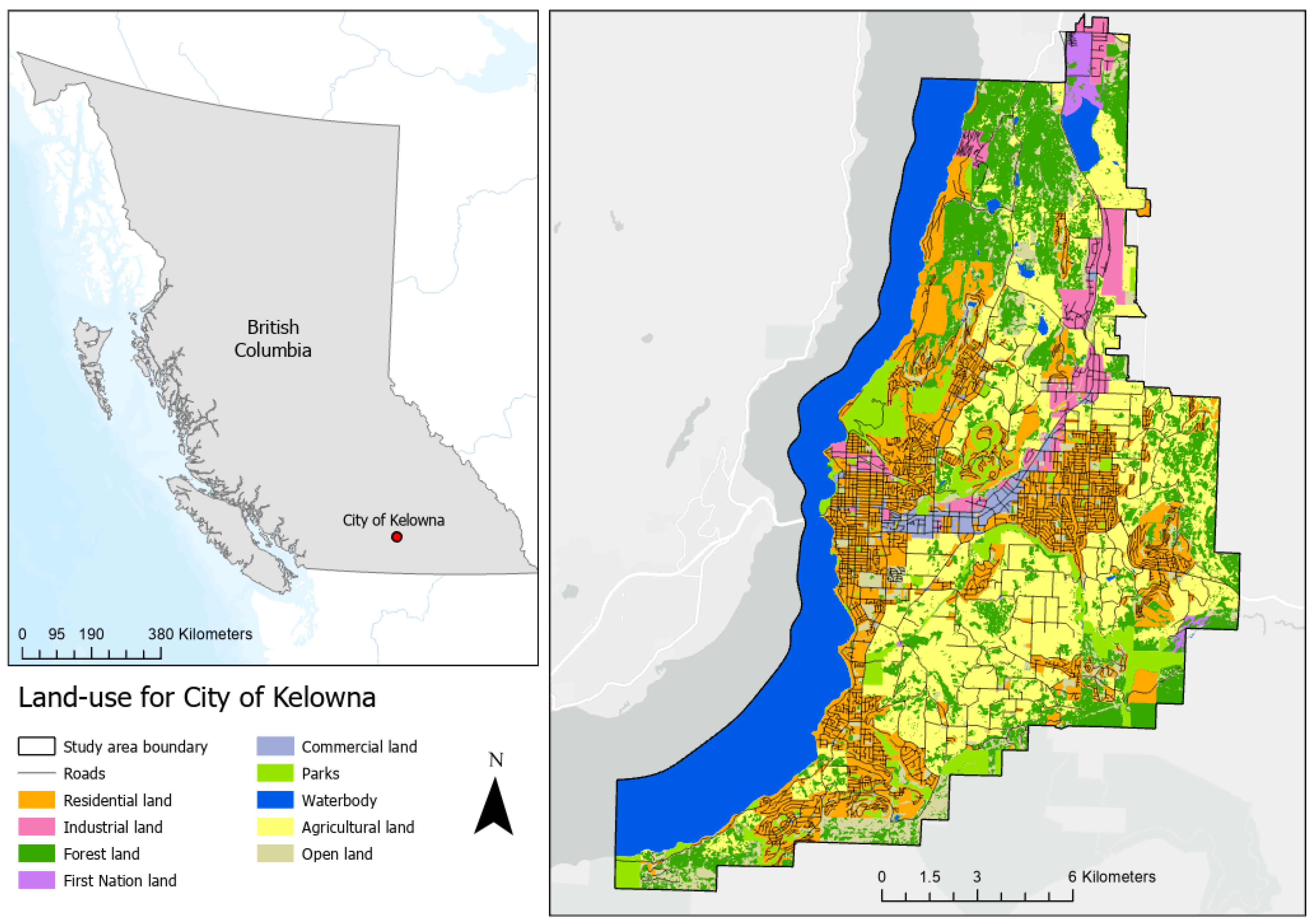
The chosen study area for this research is the City of Kelowna, B.C., Canada (Figure 2), due to its fast urban development. The City of Kelowna is situated along the eastern shore of Okanagan Lake and is surrounded by a diverse landscape that includes urban areas, agricultural lands, forests, waterbodies, and First Nation land. The city experienced significant population growth of 14% between 2016 and 2021, making it one of the fastest-growing cities in Canada [38]. As a result, the municipality faces significant challenges related to new urban developments due to its surrounding natural environment and agricultural lands.
The geospatial data collected for this research are obtained from various sources, including City of Kelowna Open Data [39], B.C. Open Data [40], and Open Government Canada [41,42,43]. This comprehensive dataset encompasses information on road networks, zoning, elevation, topography, infrastructure distribution, demographic statistics for the year 2016, as well as land-use and land cover (LULC) data. The LULC data for the years 2015 and 2020 are used exclusively for the needs of training and testing ML techniques. All geospatial data are rasterized to a 30m spatial resolution and are set in the Transverse Mercator projection with the NAD 1983 UTM Zone 11 N coordinate system.

2.2. Selection of Criteria and Suitability Functions

Eleven criteria presented in Table 1 are selected as the most important factors contributing to new urban development in general and within the City of Kelowna. Using the Euclidean distance method [44], proximity to roads, commercial areas, residential areas, industrial areas, parks, waterbodies, forest, and agricultural lands are derived from the 2015 LULC data. Next, the “Elevation” and “Slope” layers are obtained from a Digital Elevation Model (DEM). Lastly, “Proximity to high population density” is derived from a population density data layer. Specifically, population densities are calculated from the 2016 Canada Census data at the Dissemination Area (DA) level using the dasymetric mapping method [45,46], which refines population distribution within each DA to residential land-use types. Based on the calculated average population density, each raster cell has been assigned a value of 1 if the population density is higher than the average and a value of 0 if it is lower than the average. In addition to the eleven criteria, there are key constraint areas where new urban development is not expected to occur that are excluded from the suitability analysis, along with existing urban areas, road networks, waterbodies, First Nation land, agricultural land reserves, and parks.
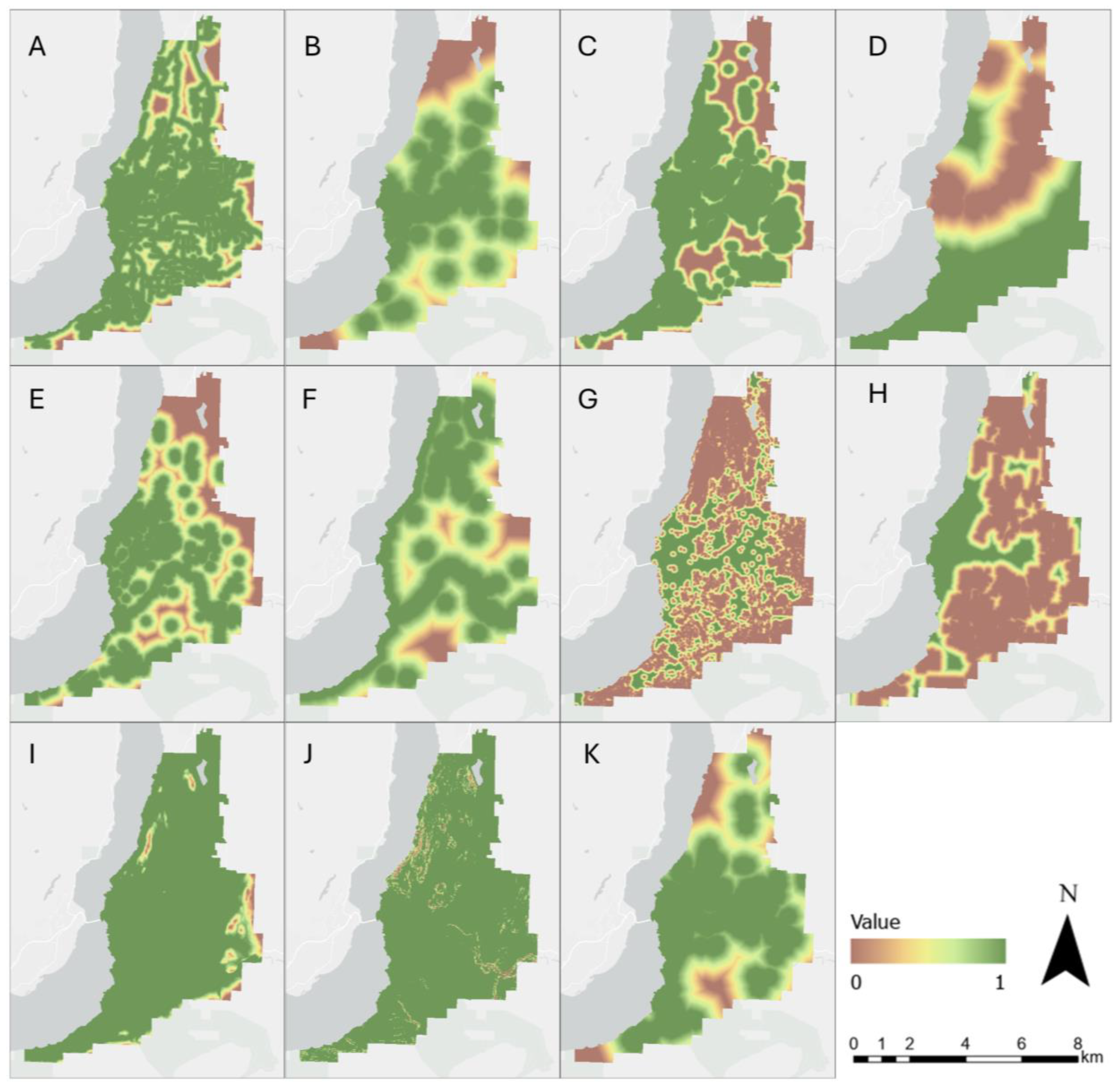
After criteria data layers are prepared, suitability functions are developed and applied to normalize each criterion. The suitability functions in breakpoint notation and their rationale are presented in Table 1. The choice of suitability function breaks is determined based on information obtained from City of Kelowna policies and scientific literature. For example, the criterion “Proximity to roads” is represented by the suitability function {(30,0), (30,1), (120,1), (900,0)} [m]. This indicates that the suitability value remains at a minimum of 0 when locations lie within 0 to 30 m from roads. Between 30 m and 120 m, the suitability value linearly increases to reach a maximum value of 1. From 120 m to 900 m, suitability declines linearly and remains 0 at locations beyond 900 m from existing roads. A value of 1 represents full satisfaction while a value of 0 represents no satisfaction. Each criteria data layer is normalized with a corresponding suitability function such that all the values range from 0 to 1 (Figure 3). The normalized data layers are then weighted and aggregated to calculate the overall suitability scores for each raster cell.

Multicollinearity of Criteria

Before proceeding with the next steps of GIS-MCE analysis, it is important to examine the interrelationships among criteria and identify possible correlations or redundancies. A multicollinearity analysis involving the calculation of Variance Inflation Factors (VIFs) [57] was applied using the following formula:
V I F = 1 1 R 2
where R 2 measures how well a given criterion can be estimated using the other criteria. A VIF equal to 1 indicates no correlation or collinearity between a given criterion and any others, while a VIF exceeding 5 suggests a high level of collinearity. The results of the VIF analysis using the normalized criteria layers data are presented in Table 2. Since no criteria exceeded a value of 5, it was concluded that no multicollinearity is present, so all criteria were included in the GIS-MCE analysis.

2.3. Criteria Weighting Approaches

This section presents in detail the approaches used for deriving criteria weights.

2.3.1. The Equal-Weights Approach

The simplest way of assigning criteria weights in MCE is by applying an EW approach, where criteria are assigned equal importance [58]. This method serves as a baseline and neutral criteria weighting approach that can be useful for procedures like sensitivity analysis [59] and facilitating suitability map comparisons [60]. In this research, the EW approach is used to enable comparisons with all other approaches. As this study considers eleven criteria, each criterion is assigned approximately 9.09% (rounding to two decimal places), summing to a total of 100%.

2.3.2. The Analytical Hierarchy Process Approach

The AHP approach involves conducting pairwise comparisons of all criteria that are relevant to a spatial problem and organizing them in a hierarchical structure [61]. In the AHP, the criteria are compared pairwise using a scale from 1 to 9, where values reflect the relative importance of one element over another. For example, a value of 1 assigned between two criteria indicates that they are considered “equally important”. Conversely, a value of 9 indicates that one criterion is “extremely important” compared to the other. The pairwise comparison is repeated for all criteria combinations to create a comparison matrix. The sum of each column of the resulting matrix is then calculated and used as a divisor for each cell in the matrix to generate new values for each matrix cell. The weight for each criterion is then calculated by taking the average of each row in the matrix. Furthermore, the Consistency Index (CI) within the AHP approach measures the consistency of the pairwise comparison judgments made by the spatial analyst or decision-maker [15,19]. Typically, a CI value less than 0.1 indicates an acceptable level of consistency in the pairwise comparisons, suggesting that the judgments are reliable. Since the relative importance of the criteria in the AHP is assigned manually, either by experts, decision-makers, or spatial analysts, it is prone to subjective judgments, biases, or incomplete information [22]. This can potentially lead to inconsistent or unreliable results for criteria weights. For this study, the relative importance of the criteria is informed by the existing literature. Table 3 presents the relative importance assigned to the criteria in the AHP pairwise comparison matrix and the derived criteria weights for the purpose of urban suitability analysis. The obtained CI value for the AHP comparisons is 0.03, indicating that the judgments involved in the pairwise comparisons are within an acceptable level of consistency.

2.3.3. The Proposed ML Approach

The proposed ML approach involves deriving criteria weights based on feature importance values from three ML techniques, namely RF, XGB, and SVM. Each technique is defined for a classification task where the training target is a binary label, with 0 indicating non-urban and 1 indicating urban locations. In this study, the impact of two training regimes on feature importance values is also explored. The training regimes and procedure for deriving criteria weights are described in the following sections.

Description of ML Training Regimes

The first training regime follows a traditional approach where the training label is derived from one map at a single timestamp, representing land use [32,34]. However, this setup tends to emphasize features related to longstanding urban developments rather than recognizing factors and conditions that were important for setting up new urban developments. As such, ML techniques may potentially be overfitted to specific features. To address this issue, a second training regime is proposed to obtain feature importance values specifically related to siting new urban developments. By including two maps to supply information about locations that have become urban, each ML technique learns to detect patterns and important features related to where new developments are most likely to occur. The proposed two-map training regime also enables each ML classifier to capture recent decision-maker priorities without the time-consuming task of acquiring expert opinions. Likewise, the two-map training regime assumes that decision-makers are better informed about the historical changes in a study area, thus allowing the ML method to capture which factors they have prioritized. The results from both training regimes are included in further steps of the MCE suitability analysis.

Evaluating Fit of ML Techniques

While feature importance values obtained from the RF, XGB, and SVM classifiers are used to derive criteria weights, direct outputs of each classifier are used to evaluate the fit of each ML technique. As such, the effects of one-map and two-map training regimes are examined for each ML type with respect to the outputs and feature importance values. The one-map training regime utilizes the eleven criteria outlined in Table 1 as the training data features, while urban and non-urban areas drawn from the 2015 LULC data supply the training target or label. In the one-map training regime, the ML techniques determine the likelihood of urban area presence given the input feature values of each training data sample. In contrast, the two-map training regime uses the same input features, while the training labels are derived from the differences between LULC data available for 2015 and 2020. In this approach, the objective of the two-map training regime is to determine the likelihood of new urban areas given the input feature values of each training data sample. This method allows ML techniques to learn the relationship between the criteria and the newly developed urban areas to derive feature importance values.

Deriving Criteria Weights Using ML Feature Importance Analysis

Once each ML technique is trained, a feature importance analysis is conducted, and resulting values are converted to criteria weights. In this study, feature importance values help in understanding the contribution of each feature to the estimation of the target label. Feature importance values are determined using properties inherent to the scikit-learn and the XGBoost classifier implementations to support the identification of which features contributed most to each classifier’s learned decision mechanisms. After feature importance values are obtained from the respective ML techniques under each training regime, each set of feature importance values is normalized so that the importance of all features sums to 1. Normalized feature importance values can then be directly used in place of criteria weights and further integrated into MCE analysis. The details of setting up the ML techniques and evaluations are presented in the following subsections.

2.3.4. Operationalizing the Proposed ML Approach

ML Techniques

The ML techniques implemented in this study include RF [62], XGB [63], and SVM [64] classifiers. The RF ensemble algorithm is a robust decision tree method capable of handling high-dimensional data. The RF technique leverages a number of decision trees that contribute to a majority vote used to obtain a final outputted value. The XGB technique is also an ensemble tree-based algorithm, instead relying on a concept called gradient boosting that involves refining a collection of weak learners at each iteration of training. XGB involves training multiple decision trees sequentially, with each tree focusing on correcting the errors of the previous one. In contrast, the SVM technique is based on a max-margin approach that aims to delineate a hyperplane to maximize separation between positive and negative training samples. To delineate the hyperplane, input features are first mapped to higher-dimension feature spaces using a kernel function. This underlying procedure enables SVM to generalize to unseen data, reducing the risk of overfitting. The RF technique benefited from the default scikit-learn parameters of the Random Forest Classifier, which creates 100 decision trees in the ensemble. Next, the number of XGB estimators was set to 100 and the maximum tree depth was set to 5. Lastly, a linear kernel was used for SVM and the regularization parameter (C) was set to 1.

Preparing ML Training Datasets

The next step requires the preparation of a training dataset. A training dataset consists of two components: training features and a training label. Training features are the independent variables or attributes provided as inputs to ML techniques, while the training label is the dependent variable or output. To form the training dataset for the one-map training regime, training features are derived from the eleven criteria data layers. The training label denotes the presence or absence of urban land-use for the year 2015, where a binary value of 0 indicates “non-urban” and 1 indicates “urban”. To configure the training dataset for the two-map training regime, the same training features are maintained from the one-map training regime. However, the LULC data from 2015 and 2020 are used to identify new and recent urban developments. In the two-map training regime, the training label instead denotes persistent non-urban areas with a value of 0, while locations that have undergone development in the interval are assigned a value of 1. Details regarding the training configuration for both methods are listed in Table 4.
Next, a stratified random sampling approach is employed to form a balanced training dataset such that the ML techniques are not biased toward majority samples. The sampling approach is based on previous studies that mitigated imbalances by ensuring there are equal numbers of positive and negative targets for the ML techniques to learn [35,65]. Specifically, 2000 points are sampled from the study area, where 50% of the training dataset labels have a value of 0 and the latter have a value of 1. This is to ensure the training dataset is balanced to mitigate ML biases toward the majority label in both the one-map and two-map methods [35]. The training samples are subsequently split into training and testing sets, with 70% of the points being used to fit the ML techniques and the remaining 30% reserved for testing [66,67].

Evaluation of ML Techniques

To evaluate the ML classifier parameterization and quality of fit, assessments were conducted with respect to the withheld testing dataset. The assessment involves using both the Receiver Operating Characteristic Area Under Curve (ROC-AUC) and F1 score with their respective components, as demonstrated in previous studies [29,35,68,69]. The emphasis of the assessment is to confirm that the ML techniques trained with one-map and two-map training regimes are operational for the respective tasks as opposed to comparing or optimizing predictive accuracy or performance.
The ROC-AUC score relies on the True Positive Rate (TPR) and the False Positive Rate (FPR). The TPR, also known as “recall”, quantifies the proportion of true positive (TP) predictions or correctly classified positives relative to all TP predictions and false negative predictions (FN) [35]. Meanwhile, the FPR represents the proportion of false positive predictions (FP) relative to all actual negatives, which includes FP and True Negative (TN). The ROC curve depicts the relationship between the TPR and FPR of ML outcomes, serving as a graphical representation for assessing the performance of a binary ML classifier. Values obtained from calculating the area under the ROC curve (ROC-AUC) range from 0 to 1, with higher values indicating better ML performance. An ROC-AUC of 0.5 implies that the ML technique performs no better than random guessing, and a value of 1.0 signifies perfect classification [70]. The F1 score is determined using precision and recall. Precision equals the ratio of TP to all positive results (TP+FP), which includes those that were misidentified. The F1 score provides a single measure that balances precision and recall. Resulting values similarly adhere to a range of 0 to 1, where 1 indicates perfect precision and 0 indicates that the ML classifier could not classify any data sample correctly [71].

2.4. Deriving Suitability Scores and Suitability Maps

After the criteria weights are established with the various weighting approaches, the criteria represented by normalized data layers are aggregated using the WLC method to derive the final suitability score for each raster cell. The calculation of output suitability scores S r i for a spatial problem r i has been accomplished using the following WLC formula [37]:
S r i = j = 1 n w j f j r i
where w j is the weight of importance assigned to criterion j and f j r i is the suitability function for r i for the j t h criterion. The output suitability scores range from value 0 to 1, where 0 represents locations that are completely unsuitable while 1 represents the most suitable locations for the decision problem. In this study, a value of 1 indicates areas that are the most suitable for urban development. The resulting suitability scores are classified into several classes to produce suitability maps depicting locations that range from poor to excellent suitability for the new urban development in the study area. Suitability maps are derived for each weighting method for the purpose of comparison.

3. Results and Discussion

To prepare and normalize the data layers for this study, the ArcGIS Pro (version 3.2) software is used [72]. Next, the AHP criteria weights are developed using Microsoft Excel [73]. The ArcGIS Pro software was used to prepare the ML training datasets and implement the proposed ML weighing approach. Specifically, an ArcGIS Python Notebook and ArcPy [72] were used. An ArcGIS Python Notebook provides an interactive means of writing and running Python code within ArcGIS Pro. The ML approach is implemented using functions from the ArcPy, scikit-learn [74], and xgboost [63] Python libraries to prepare training datasets, to train each classifier, to perform the feature importance analysis, and to obtain the criteria weights.

3.1. Evaluating the ML Techniques

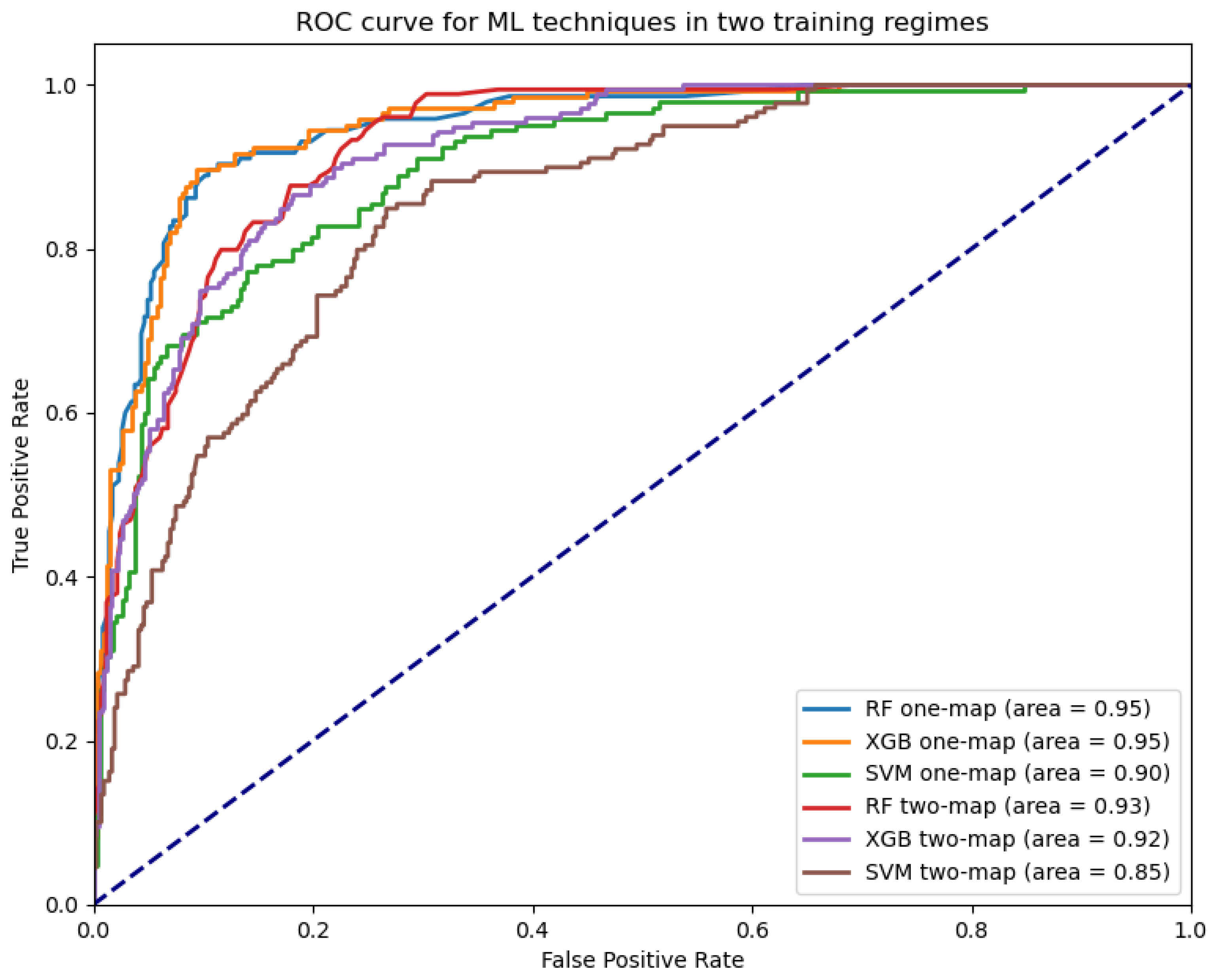
Figure 4 presents the obtained ROC curves and the AUC values for each ML technique and training regime. The high AUC values indicate that the ML techniques and their parameters have been effectively configured. As the ML techniques in this research are not intended to produce any predictions, the ROC values were determined with respect to data withheld for testing purposes presented in Section 2.3.4.
Table 5 presents the evaluation results for the ML techniques using the two different training regimes described in Section 2.3.3. Regardless of the training data setup used, RF and XGB exhibit high recall, precision, and F1 scores. Conversely, SVM’s performance under both training regimes shows lower recall scores.

3.2. Comparing Derived Criteria Weights under Each Training Regime

The criteria weights obtained from all weighting approaches, including the RF, XGB, and SVM techniques under both training regimes, are summarized in Table 6a. Additionally, Table 6b summarizes the ranking of the criteria by each approach along with the average ranking for each criterion.
Comparing the criteria rankings of the AHP and ML approaches, “Proximity to roads” consistently ranks among the top three criteria affecting urban development. Additionally, “Elevation” and “Slope” are identified as the least important criteria in the AHP, and the RF technique was trained with both one-map and two-map regimes. The overall criteria rankings from the AHP closely align with those obtained using the RF and XGB techniques under the two-map training regime. However, the SVM technique presents a different weight distribution compared to the AHP under both training regimes.
Regarding the criteria weights obtained from the proposed ML approach, RF and XGB yield very similar criteria weight outcomes while SVM presents different results in both training regimes. Under the one-map training regime, “Proximity to agricultural” is ranked as the most important criterion of both RF and XGB techniques, with a weight of over 25%. “Proximity to forest” was also allocated a high criteria weight based on its larger contribution within the RF and XGB techniques. In contrast, “Slope” was determined as the most important criterion of the SVM technique, with a normalized weight of 25.8%. The most important criteria determined with the SVM technique can indicate a different stakeholder viewpoint that prioritizes certain criteria as being the most important. For example, “Slope” is often regarded as one of the least important criteria while “Proximity to roads” is typically considered one of the most important criteria by stakeholders and decision-makers [75,76,77]. Evidently, the feature importance values obtained from ML techniques trained under the one-map training regime are influenced by longstanding urban locations in the City of Kelowna. As such, the one-map training regime may have limited applicability regarding uncovering factors associated with favorable new urban development locations in real-world decision-making processes.
In contrast, the goal of the two-map training regime was to obtain feature importance values that take new urban developments into consideration (Table 4). By accounting for the actual recent study area changes that occurred between two timesteps, the obtained values can be seen as reflections of the choices of criteria weights developed by stakeholders and decision-makers. As such, the “Proximity to roads” criterion was identified as the most important criterion of both the RF and XGB techniques (Table 6). “Proximity to high population density” is also ranked higher in both techniques trained using the two-map training regime. The criteria weights associated with the SVM technique also are more realistic regarding “Proximity to roads,” which ranked as the second most important, while “Slope” was allocated less weight. By comparing the criteria weights obtained under the two-map training regime with those specified manually in previous studies, the proposed ML approach reduces the difficulties of criteria weight derivation.
After comparing the criteria weights attributed to each ML technique under both training regimes, the two-map training regime is considered to be a better-informed approach for training ML techniques, obtaining feature importance values and deriving criteria weights for the task of determining suitable locations for new urban developments. Therefore, the criteria weights associated with the two-map ML techniques are further compared with the traditional approaches in the subsequent sections.

3.3. Comparing Effects of Sample Size on Derived Criteria Weights

Additional tests have been conducted to determine if the number of training points influences the outputs of the ML techniques. For example, the RF technique was trained using the two-map regime with 2000, 4000 and 6000 training points. The results demonstrate consistent criteria weight distributions and rankings (Table 7) regardless of the choice of number of training points. This is consistent with findings from [78], which found that lower numbers of training data samples even improved outcomes. Therefore, the presented results following this section are produced using 2000 data samples to train each ML technique.

3.4. Analyzing Obtained Suitability Maps

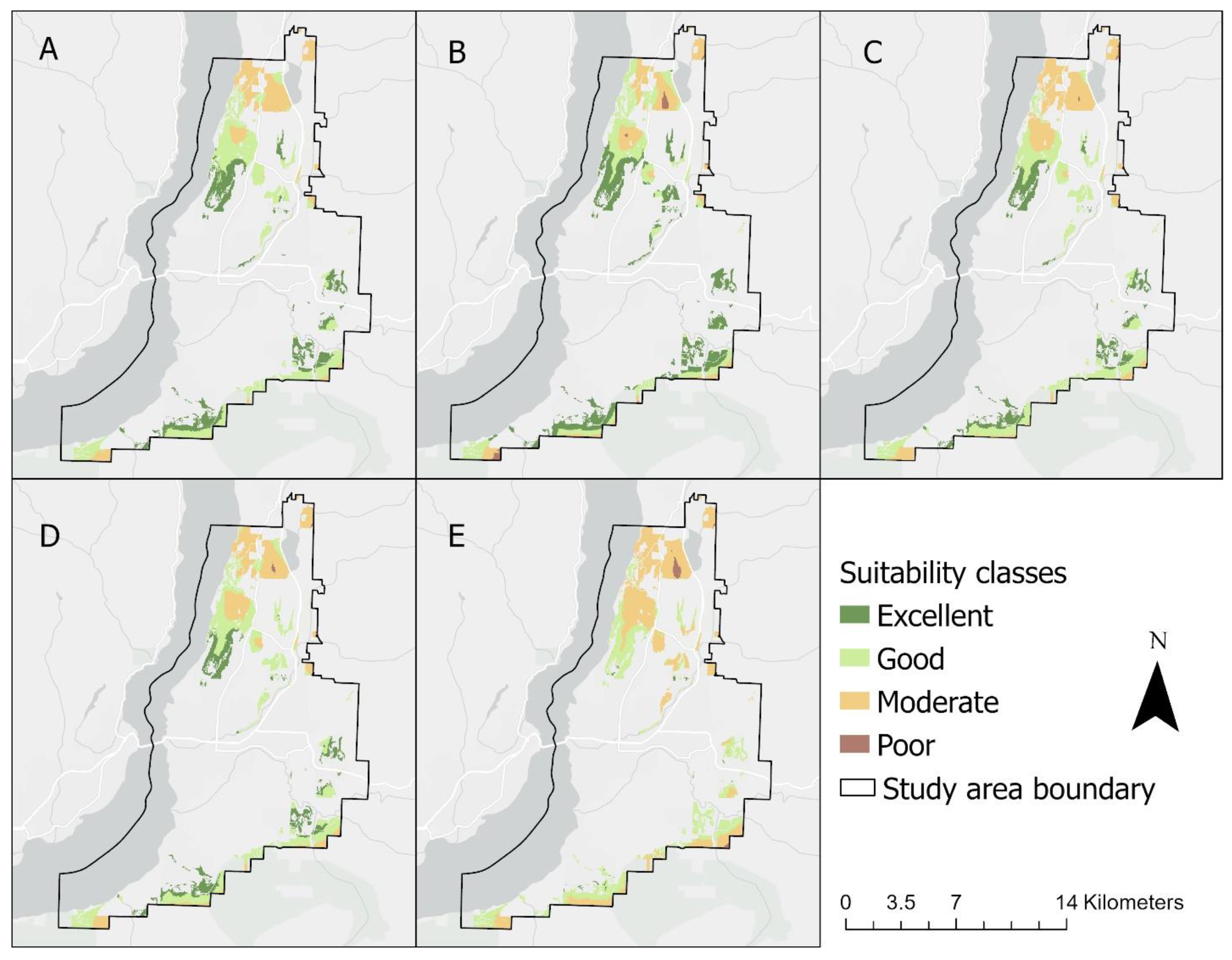
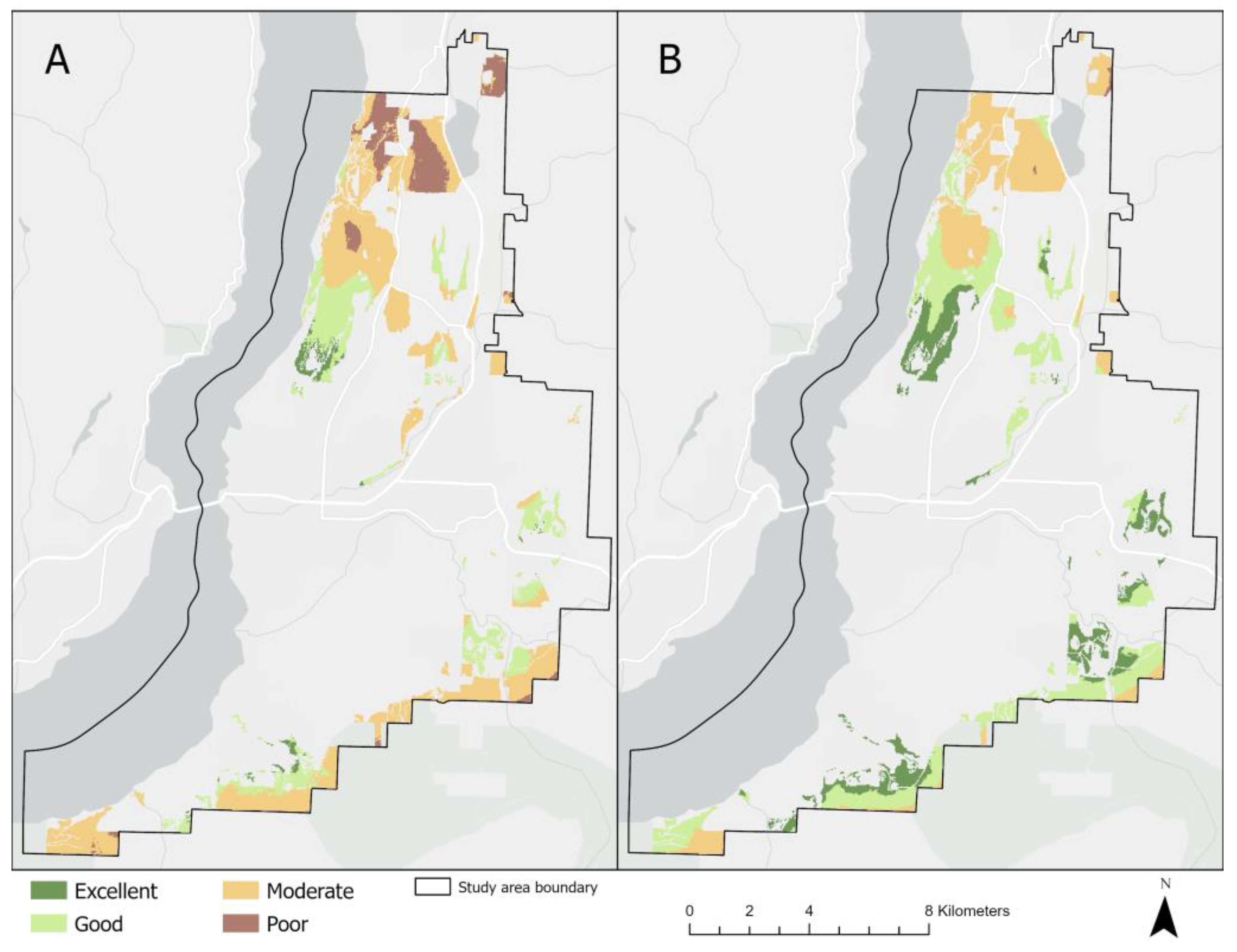
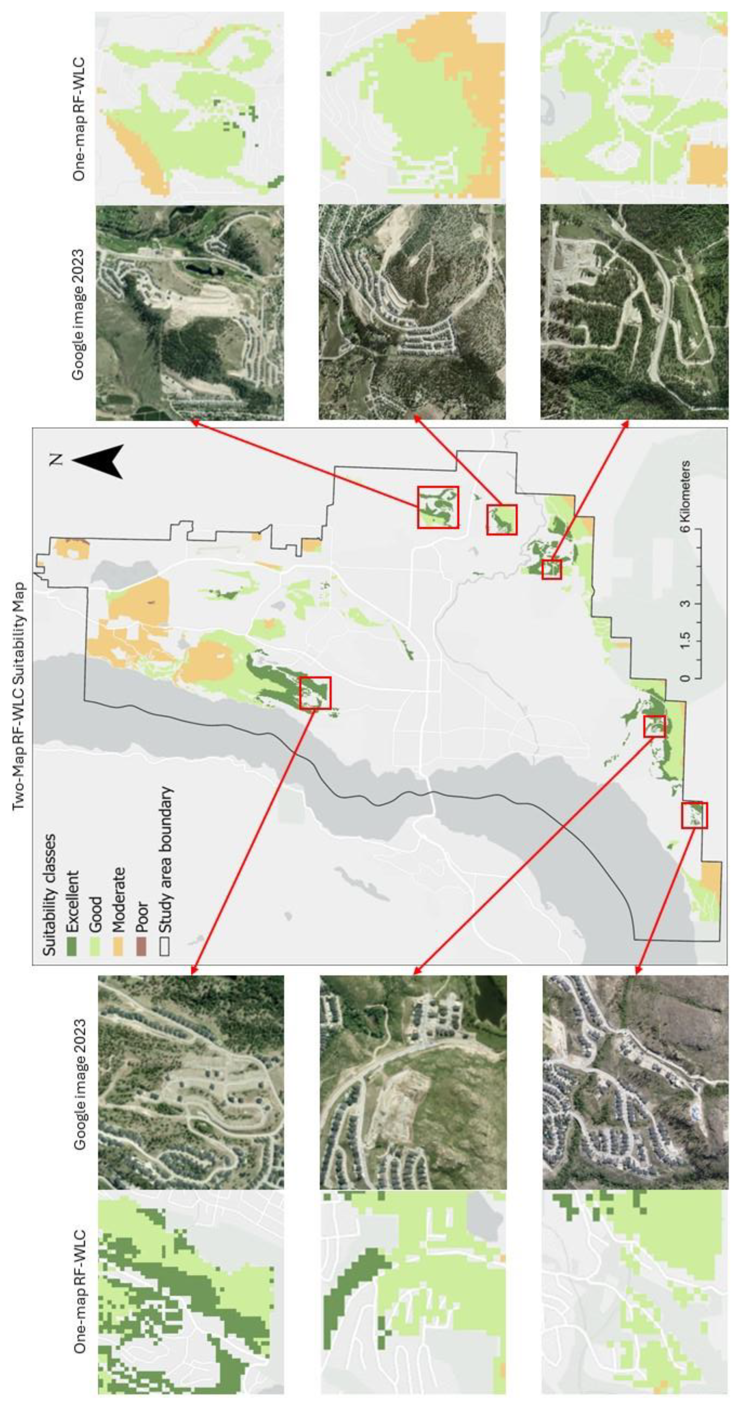
After integrating the criteria weights using the WLC aggregation method, the obtained suitability scores are classified into four classes using the equal interval classification method. The classes are defined as follows: excellent (0.76–1.00), good (0.51–0.75), moderate (0.26–0.50), and poor (0.0–0.25) suitability for urban development. Figure 5 presents suitability maps created using criteria weights derived from the EW, AHP, and respective ML techniques trained with the two-map regime in the WLC aggregation method. Areas classified as having excellent suitability are interpreted as having the highest potential for future urban development. At the other extreme, “poor” suitability indicates areas unsuitable for new urban developments within the study area. For comparison purposes, suitability maps produced using the criteria weights obtained from the RF-WLC approach under both one-map and two-map training regimes are presented in Figure 6 to support visual assessments of the effects of the training data methods.
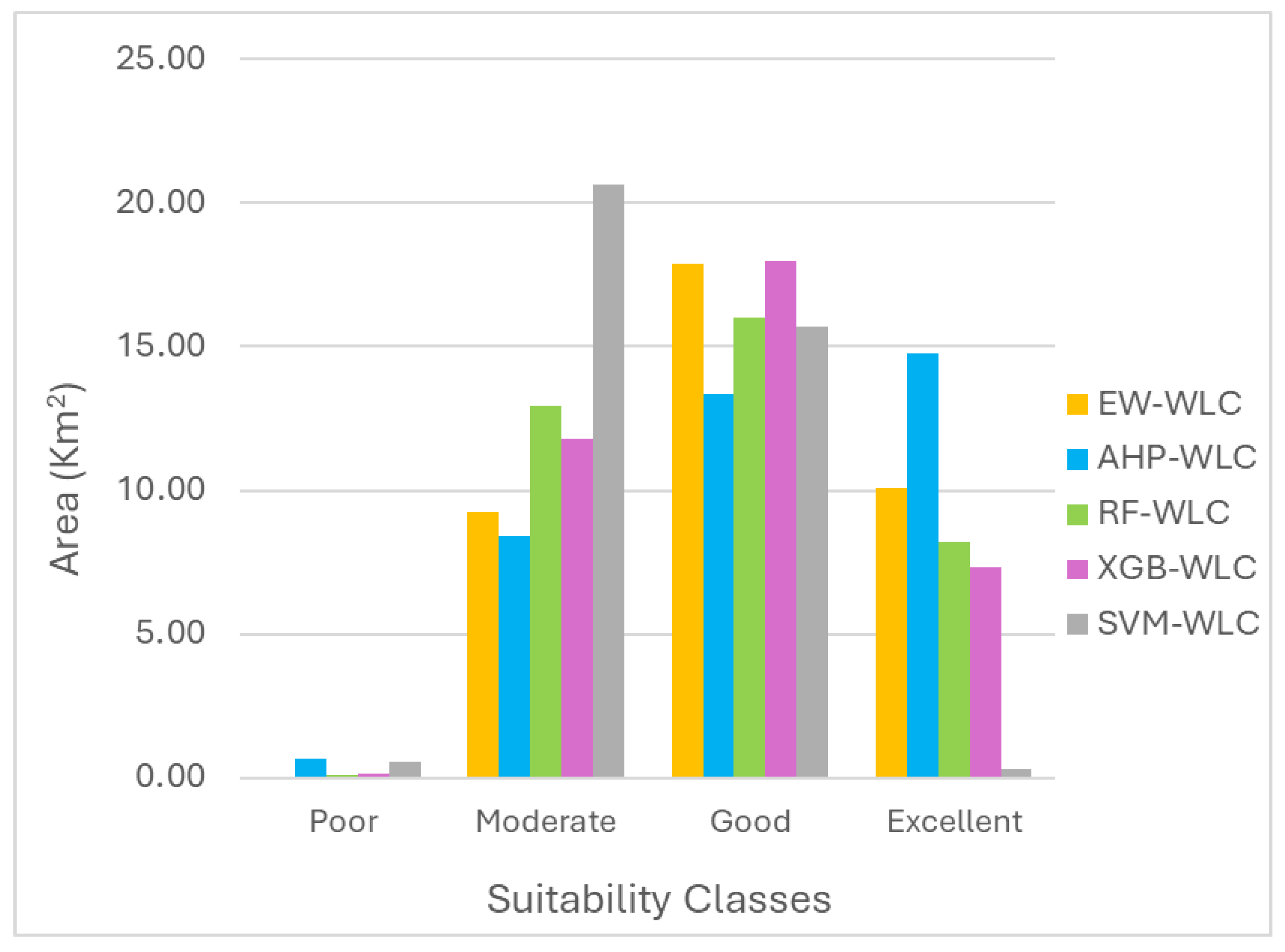
Additionally, the surface area (in km2) of derived suitability for each class is summarized in Figure 7 and Table 8 to quantify the differences between the various weighting approaches. The EW approach identified the smallest amount of “poor suitability” area and a moderate amount of area classified as excellent. Conversely, the suitability map created with the AHP-WLC approach shows the largest area as having excellent suitability, almost double that of the RF-WLC and XGB-WLC approaches. The RF-WLC and XGB-WLC approaches demonstrate similar values for surfaces under the same suitability classes. On the other hand, the SVM-WLC approach presents a distinct outcome compared to the other approaches. The outcome generated using the SVM-WLC approach depicts the least area as having “excellent” suitability, almost close to zero, with most of the area classified as having “moderate” suitability.

3.5. Comparing Suitability Maps

Results from GIS-MCE analysis, such as suitability scores and maps, are typically used in further deliberations of stakeholders to guide decision-making processes. Given that developing suitability maps is not equivalent to making predictions of new land-use states, the techniques for validating suitability maps are limited. Instead, suitability maps serve as a starting point for stakeholder discussions that would lead to final decisions about where new urban developments should be sited. Nevertheless, to compare the suitability maps developed with the various approaches, the respective outcomes are examined using visual and areal cross-comparison techniques, the Kappa Index of Agreement (KIA), and a visual comparison with recent real-world imagery obtained for the City of Kelowna.

3.5.1. Suitability Map Cross-Comparison

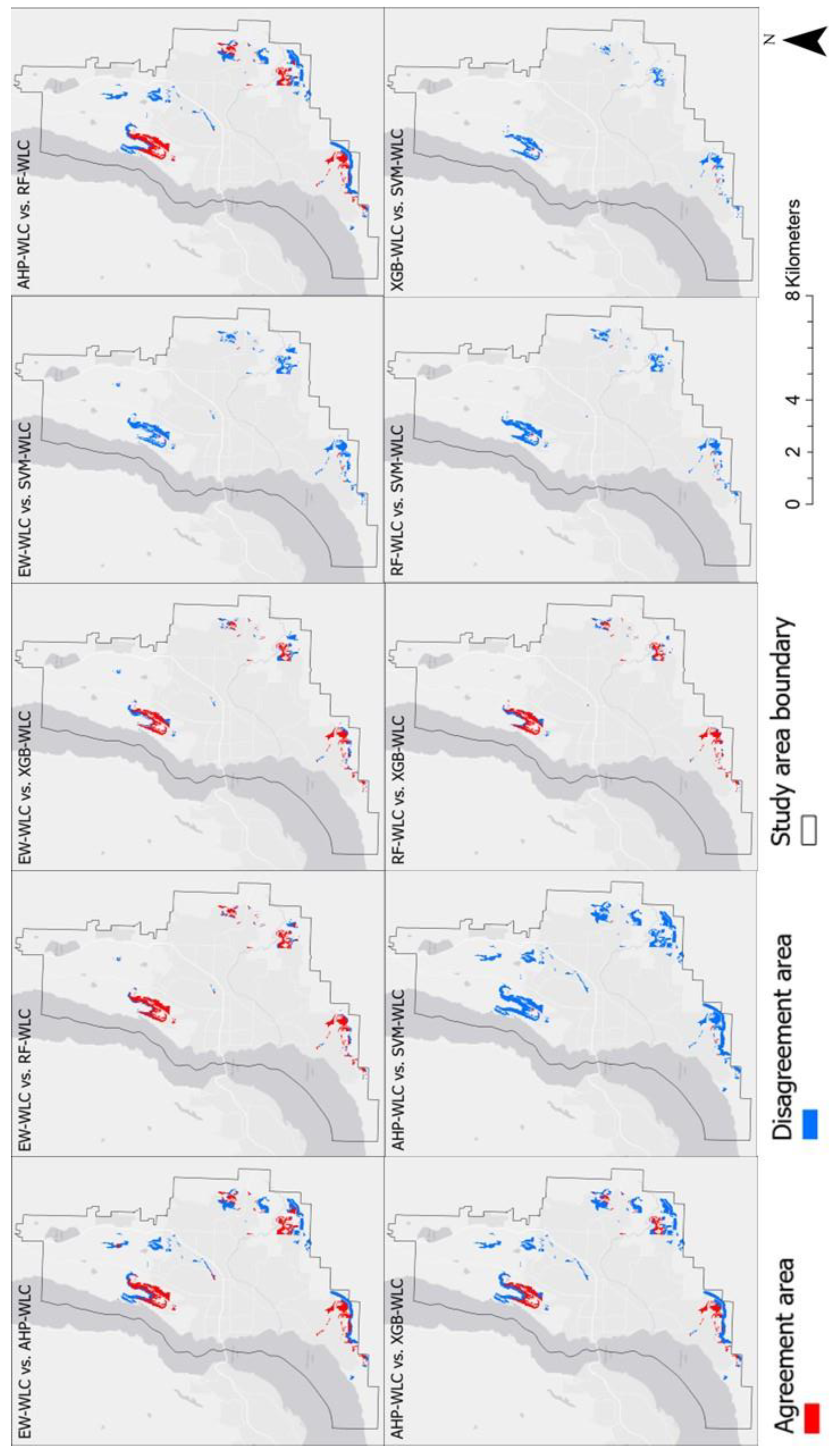
The cross-comparison technique [79] was used to generate the agreement/disagreement maps with respect to the “excellent” suitability class for all criteria weighting methods. Focusing on comparing the “excellent” class is important because potential stakeholders and urban developers will be the most interested in locations identified as having the highest suitability for new urban developments. The EW-WLC map is used as a neutral suitability map by which to base the comparisons. Figure 8 presents the cross-comparison maps obtained from each weighting approach with the WLC method, indicating locations where the highest suitability scores obtained overlap or differ. The areas in agreement are shown in red, while disagreeing areas are shown in blue on the maps. Overall, it can be observed that SVM-WLC generates the smallest area with “excellent” suitability and shows the most disagreement with all other approaches. Conversely, the AHP-WLC map depicts the largest area under the “excellent” suitability class (Figure 7, Table 8) while simultaneously showing a significant amount of locational disagreement with other approaches (Figure 8). Regardless, the RF-WLC and XGB-WLC show the most agreement with this suitability class among all MCE approaches.
With respect to the neutral baseline (EW-WLC), both the RF-WLC and XGB-WLC approaches exhibit high agreement between “excellent” areas. The similarities between EW-WLC, RF-WLC, and XGB-WLC can be attributed to the selection of criteria and several local trends observed in transformed values of factors (Figure 3). For example, “Proximity to Roads” and “Proximity to Residential” display similarly high values in some areas, thus contributing to the observation that the EW-WLC approach has assigned “Excellent” suitability classes to several similar areas identified via the RF-WLC and XGB-WLC approaches. Meanwhile, both the RF-WLC and XGB-WLC approaches assign “Proximity to Roads” one of the highest criteria weights. Due to the numerous combinations of criteria weights that can lead to an “excellent” class being assigned to certain areas by the EW-WLC approach, this demonstrates the importance of comparing criteria weights with the existing literature (Section 3.2) and the need for inspections of the local factor values contributing to high suitability values. Despite the observed local similarities between the RF-WLC and XGB-WLC approaches with the neutral baseline, the agreement with other suitability classes deviates, as observed in Figure 5.

3.5.2. Quantifying Agreement between Suitability Maps

Following the visual and areal cross-comparisons of each suitability map, the similarity between the suitability class locations in each pair of maps is quantified using the Kappa Index of Agreement (KIA) [52,80,81] given that suitability maps are not the result of a space-time process. KIA values are presented in Table 9 and, when approaching 1, suggest high agreement between suitability classes present in the two maps being compared. Conversely, KIA values approaching 0 indicate low alignment of suitability classes at most locations compared across the study region.
Across each pair of compared suitability maps, the KIA values confirm previous evaluations. Additionally, the KIA values further confirm the similarities between the suitability maps attributed to the RF and XGB techniques. For example, RF-WLC and XGB-WLC exhibit the highest agreement of any pair of suitability maps based on the KIA value of 0.90 (Table 9). In contrast the SVM-WLC map is associated with the lowest KIA values obtained from all suitability map comparisons. The minimum KIA value (0.32) is associated with the comparison between AHP-WLC and SVM-WLC, indicating that these two maps exhibit the least similarity of suitability class locations across the study region. Considering the KIA values attributed to the overall comparisons of EW-WLC and RF-WLC (0.84), and EW-WLC and XGB-WLC (0.83), the deviating locational agreement between suitability classes other than “excellent” as previously discussed (Section 3.5.1) are also confirmed.

3.5.3. Examining Suitability Maps versus Real-World Images

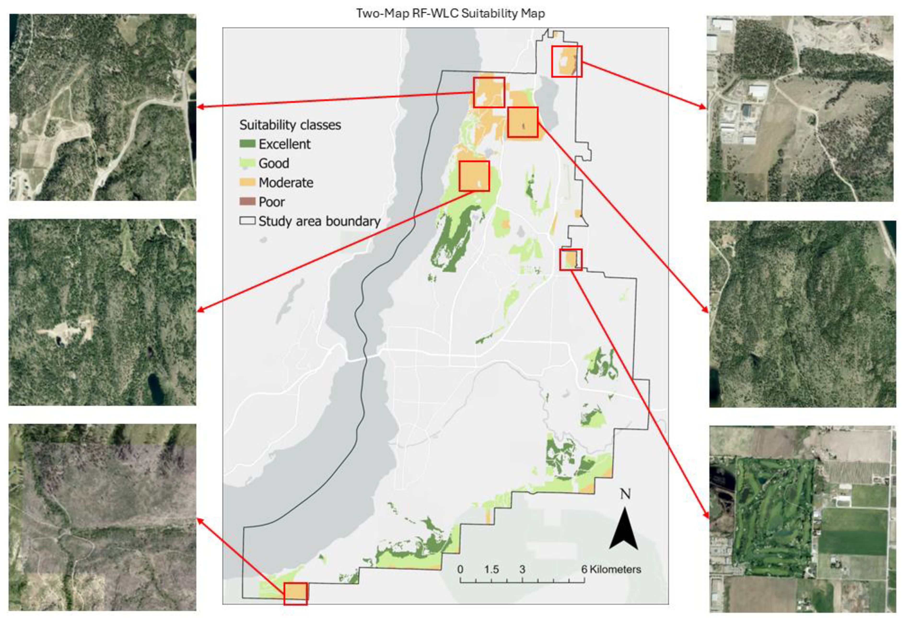
In order to confirm the applicability of the proposed ML-MCE method and obtained suitability scores, a manual visual verification with an alternative source of “field observations” is conducted with respect to recent Google Earth satellite imagery. As the RF-WLC yields very similar results to XGB-WLC and attained the highest ROC-AUC score among the ML techniques trained under the two-map regime, the RF-WLC suitability map was compared to areas with and without recent urban developments in the study area. Figure 9 presents a comparison of the RF-WLC suitability map with real-world satellite imagery from 2023, focusing on areas of “moderate” and “poor” suitability. The highlighted locations identified to have low suitability show that no urban development has occurred since. This also suggests that the RF-WLC suitability map concurs with knowledge about the criteria. For example, areas determined to be less accessible (Figure 3A), more isolated from current urban developments (Figure 3C), and closer to industrial zones (Figure 3D) are appropriately identified as less suitable for new urban developments.
Next, Figure 10 presents a comparison of the suitability maps obtained with the RF-WLC approach trained under both the one- and two-map regimes versus real-world satellite imagery for the year 2023. Focusing on the areas of “excellent” suitability, the visual assessment indicates that areas identified as highly suitable for new urban developments using the two-map RF-WLC approach corresponded with some recent new urban developments in the study area. Overall, the visual assessment further confirms that the two-map training regime for ML techniques is well suited for deriving criteria weights in the proposed ML-MCE method. In contrast, the RF-WLC suitability maps attributed to the one-map training regime show that many of the selected locations do not have the highest suitability scores. This suggests that urban developers and planners in the City of Kelowna are indeed considering the areas with characteristics or criteria identified with the two-map ML-MCE methodology proposed in this study.

3.6. Limitations and Future Directions

Although the comparison of ML techniques and training regimes showed the value of deriving criteria weights with two timesteps for urban development suitability, there remain several limitations and opportunities for improvement. In real-world implementation, ML techniques and software may not be widely accessible to urban planners, as the proper setup, training, and testing of ML techniques may be a challenge for municipal planners. Next, while the four-class equal interval breaks used to assign suitability classes are easier to visualize and understand, the real variation of the suitability values obtained from each approach require additional comparisons at finer-level classes or on a continuous scale in future studies. Another limitation of this work is that the WLC method used in this study is based on a Simple Additive Scoring (SAS) method, which takes the mean of all the components in the analysis [75]. When the number of criteria increases, the importance of criteria decreases, oversimplifying the decision-making process of many complex spatial problems like urban land-use suitability analysis. To overcome this issue in future studies, a more complex MCE method can be applied, such as the Ordered Weighted Averaging (OWA) or Logic Scoring of Preference (LSP) methods. Another limitation of this study is that it only considered eleven criteria, while complex urban planning spatial decision problems may require a much larger number of criteria, especially for larger study areas and urban metropolitan regions. Investigating the limits of the number of criteria remains unexplored with the ML-MCE method and could be explored in future work. Lastly, the ML techniques in this study are trained using the same normalized criteria data layers used for the EW and AHP approaches. Future studies should explore and compare the effects of integrating domain knowledge in data layer pre-processing procedures versus standard ML data normalization strategies.

4. Conclusions

This research explores the integration of ML with GIS-MCE for determining criteria weights and with the aim to analyze urban development suitability. Focusing specifically on a case study in the City of Kelowna, results indicate that approaches such as the neutral EW and the traditional AHP produce different criteria weights than weights obtained via feature importance analyses of the three ML techniques. Among the ML techniques explored, the criteria weights derived from RF feature importance values closely aligned with those of XGB, while SVM shows markedly different criteria weights. Additionally, this study examined the differences in criteria weights, distributions, and rankings that result from different training regimes. A traditional one-map training regime for ML techniques is compared with the proposed two-map training regime for deriving feature importance related to new urban developments specifically. The results demonstrate that the two-map training regime is more suitable for this case study and enables criteria weights that are more likely to align with perspectives of potential stakeholders and urban planners. After comparing the suitability maps created using the RF-WLC approach with the 2023 Google Earth satellite images, the visual assessments confirmed the effectiveness of the proposed ML-MCE method in real-world urban planning in the City of Kelowna.
Overall, the proposed ML-MCE method provides a novel, data-driven, and systematic framework for combining geospatial data and ML techniques for urban development suitability analysis. This framework has the potential to assist in city planning and urban land-use management by supporting decision-makers.

Author Contributions

Conceptualization, Formal Analysis, Investigation, Methodology, Original draft, Review and Editing L.Q.Z., A.v.D. and S.D.; Funding Acquisition, Supervision, Suzana Dragicevic; Software, L.Q.Z. and A.v.D. All authors have read and agreed to the published version of the manuscript.

Funding

This research was funded by the Natural Sciences and Engineering Research Council (NSERC) of Canada Graduate Scholarships Master’s Program (CGSM) scholarship and Discovery Grant (RGPIN-2023-04052) awarded to the first and third authors, respectively.

Data Availability Statement

Publicly available datasets were used in this study. The data can be found at https://opendata.kelowna.ca/ (accessed on 3 July 2023) (City of Kelowna Zoning data, Road Networks data), https://open.canada.ca/data/en/dataset/4e615eae-b90c-420b-adee-2ca35896caf6 (accessed on 3 July 2023) (Canada Land-use and Land Cover data 2015, 2020), https://open.canada.ca/data/en/dataset/d0cdef71-9343-46c3-b2e7-c1ded5907686 (accessed on 3 July 2023) (Canada Lakes and Rivers Boundaries data), https://open.canada.ca/data/en/dataset/7f245e4d-76c2-4caa-951a-45d1d2051333 (accessed on 3 July 2023) (Canadian DEM data), https://www12.statcan.gc.ca/census-recensement/2021/geo/index-eng.cfm (accessed on 3 July 2023) (Canadian Census data), and https://catalogue.data.gov.bc.ca/dataset/alc-alr-polygons/resource/d35b18b0-ecfa-468b-b31a-2bf16a459a7c (accessed on 3 July 2023) (BC Agricultural Land Reserve data).

Acknowledgments

The authors are grateful for the full support of the Natural Sciences and Engineering Research Council of Canada (NSERC). The authors are also thankful for the constructive comments provided by two anonymous reviewers.

Conflicts of Interest

The authors have no conflicts of interest to declare.

References

  1. Malczewski, J. GIS-based Multicriteria Decision Analysis: A Survey of the Literature. Int. J. Geogr. Inf. Sci. 2006, 20, 703–726. [Google Scholar] [CrossRef]
  2. Malczewski, J.; Jankowski, P. Emerging Trends and Research Frontiers in Spatial Multicriteria Analysis. Int. J. Geogr. Inf. Sci. 2020, 34, 1257–1282. [Google Scholar] [CrossRef]
  3. Chen, J. GIS-Based Multi-Criteria Analysis for Land Use Suitability Assessment in City of Regina. Environ. Syst. Res. 2014, 3, 13. [Google Scholar] [CrossRef]
  4. Gelan, E. GIS-Based Multi-Criteria Analysis for Sustainable Urban Green Spaces Planning in Emerging Towns of Ethiopia: The Case of Sululta Town. Environ. Syst. Res. 2021, 10, 13. [Google Scholar] [CrossRef]
  5. Masoudi, M.; Aboutalebi, M.; Asrari, E.; Cerdà, A. Land Suitability of Urban and Industrial Development Using Multi-Criteria Evaluation (MCE) and A New Model by GIS in Fasa County, Iran. Land 2023, 12, 1898. [Google Scholar] [CrossRef]
  6. Abid, S.K.; Sulaiman, N.; Chan, S.W.; Nazir, U.; Abid, M.; Han, H.; Ariza-Montes, A.; Vega-Muñoz, A. Toward an Integrated Disaster Management Approach: How Artificial Intelligence Can Boost Disaster Management. Sustainability 2021, 13, 12560. [Google Scholar] [CrossRef]
  7. Masoudi, M.; Centeri, C.; Jakab, G.; Nel, L.; Mojtahedi, M. GIS-Based Multi-Criteria and Multi-Objective Evaluation for Sustainable Land-Use Planning (Case Study: Qaleh Ganj County, Iran) “Landuse Planning Using MCE and Mola”. Int. J. Environ. Res. 2021, 15, 457–474. [Google Scholar] [CrossRef]
  8. Dai, L.; Zhao, X.; He, H.S.; Deng, H.; Yu, D.; Zhou, L.; Wu, S. Evaluating Land-Use Suitability of an Industrial City in Northeast China. Int. J. Sustain. Dev. World Ecol. 2008, 15, 378–382. [Google Scholar] [CrossRef] [PubMed]
  9. Abebe, M.T.; Megento, T.L. Urban Green Space Development Using GIS-Based Multi-Criteria Analysis in Addis Ababa Metropolis. Appl. Geomat. 2017, 9, 247–261. [Google Scholar] [CrossRef]
  10. Liu, R.; Zhang, K.; Zhang, Z.; Borthwick, A.G.L. Land-Use Suitability Analysis for Urban Development in Beijing. J. Environ. Manag. 2014, 145, 170–179. [Google Scholar] [CrossRef] [PubMed]
  11. Zhang, X.; Fang, C.; Wang, Z.; Ma, H. Urban Construction Land Suitability Evaluation Based on Improved Multi-Criteria Evaluation Based on GIS (MCE-GIS): Case of New Hefei City, China. Chin. Geogr. Sci. 2013, 23, 740–753. [Google Scholar] [CrossRef]
  12. Caprioli, C.; Bottero, M. Addressing Complex Challenges in Transformations and Planning: A Fuzzy Spatial Multicriteria Analysis for Identifying Suitable Locations for Urban Infrastructures. Land Use Policy 2021, 102, 105147. [Google Scholar] [CrossRef]
  13. Chen, Y.; Yu, J.; Khan, S. Spatial Sensitivity Analysis of Multi-Criteria Weights in GIS-Based Land Suitability Evaluation. Environ. Model. Softw. 2010, 25, 1582–1591. [Google Scholar] [CrossRef]
  14. Feick, R.; Hall, B. A Method for Examining the Spatial Dimension of Multi-Criteria Weight Sensitivity. Int. J. Geogr. Inf. Sci. 2004, 18, 815–840. [Google Scholar] [CrossRef]
  15. Saaty, T.L. A Scaling Method for Priorities in Hierarchical Structures. J. Math. Psychol. 1977, 15, 234–281. [Google Scholar] [CrossRef]
  16. Hwang, C.-L.; Yoon, K. Multiple Attribute Decision Making; Lecture Notes in Economics and Mathematical Systems; Springer: Berlin/Heidelberg, Germany, 1981; Volume 186, ISBN 978-3-540-10558-9. [Google Scholar]
  17. Shannon, C.E. A Mathematical Theory of Communication. Bell Syst. Tech. J. 1948, 27, 379–423. [Google Scholar] [CrossRef]
  18. Greene, R.; Luther, J.E.; Devillers, R.; Eddy, B. An Approach to GIS-Based Multiple Criteria Decision Analysis That Integrates Exploration and Evaluation Phases: Case Study in a Forest-Dominated Landscape. For. Ecol. Manag. 2010, 260, 2102–2114. [Google Scholar] [CrossRef]
  19. Saaty, T.L. The Analytic Hierarchy Process: Decision Making in Complex Environments. In Quantitative Assessment in Arms Control: Mathematical Modeling and Simulation in the Analysis of Arms Control Problems; Avenhaus, R., Huber, R.K., Eds.; Springer: Boston, MA, USA, 1984; pp. 285–308. ISBN 978-1-4613-2805-6. [Google Scholar]
  20. Clark Labs TerrSet. Available online: https://clarklabs.org/terrset/ (accessed on 10 September 2023).
  21. Esri ArcMap. Available online: https://www.esri.com/en-us/arcgis/products/arcgis-desktop/resources (accessed on 10 September 2023).
  22. Liu, Y.; Eckert, C.M.; Earl, C. A Review of Fuzzy AHP Methods for Decision-Making with Subjective Judgements. Expert Syst. Appl. 2020, 161, 113738. [Google Scholar] [CrossRef]
  23. Dodevska, Z.; Radovanović, S.; Petrović, A.; Delibašić, B. When Fairness Meets Consistency in AHP Pairwise Comparisons. Mathematics 2023, 11, 604. [Google Scholar] [CrossRef]
  24. Choi, Y. GeoAI: Integration of Artificial Intelligence, Machine Learning, and Deep Learning with GIS. Appl. Sci. 2023, 13, 3895. [Google Scholar] [CrossRef]
  25. Chaturvedi, V.; de Vries, W.T. Machine Learning Algorithms for Urban Land Use Planning: A Review. Urban Sci. 2021, 5, 68. [Google Scholar] [CrossRef]
  26. Huang, M.; Gong, D.; Zhang, L.; Lin, H.; Chen, Y.; Zhu, D.; Xiao, C.; Altan, O. Spatiotemporal Dynamics and Forecasting of Ecological Security Pattern under the Consideration of Protecting Habitat: A Case Study of the Poyang Lake Ecoregion. Int. J. Digit. Earth 2024, 17, 2376277. [Google Scholar] [CrossRef]
  27. Chang, Z.; Du, Z.; Zhang, F.; Huang, F.; Chen, J.; Li, W.; Guo, Z. Landslide Susceptibility Prediction Based on Remote Sensing Images and GIS: Comparisons of Supervised and Unsupervised Machine Learning Models. Remote Sens. 2020, 12, 502. [Google Scholar] [CrossRef]
  28. Janiec, P.; Gadal, S. A Comparison of Two Machine Learning Classification Methods for Remote Sensing Predictive Modeling of the Forest Fire in the North-Eastern Siberia. Remote Sens. 2020, 12, 4157. [Google Scholar] [CrossRef]
  29. Garzón, M.B.; Blazek, R.; Neteler, M.; de Dios, R.S.; Ollero, H.S.; Furlanello, C. Predicting Habitat Suitability with Machine Learning Models: The Potential Area of Pinus Sylvestris L. in the Iberian Peninsula. Ecol. Model. 2006, 197, 383–393. [Google Scholar] [CrossRef]
  30. Taghizadeh-Mehrjardi, R.; Nabiollahi, K.; Rasoli, L.; Kerry, R.; Scholten, T. Land Suitability Assessment and Agricultural Production Sustainability Using Machine Learning Models. Agronomy 2020, 10, 573. [Google Scholar] [CrossRef]
  31. Al-Ruzouq, R.; Shanableh, A.; Yilmaz, A.G.; Idris, A.; Mukherjee, S.; Khalil, M.A.; Gibril, M.B.A. Dam Site Suitability Mapping and Analysis Using an Integrated GIS and Machine Learning Approach. Water 2019, 11, 1880. [Google Scholar] [CrossRef]
  32. Al-Ruzouq, R.; Abdallah, M.; Shanableh, A.; Alani, S.; Obaid, L.; Gibril, M.B.A. Waste to Energy Spatial Suitability Analysis Using Hybrid Multi-Criteria Machine Learning Approach. Environ. Sci. Pollut. Res. 2022, 29, 2613–2628. [Google Scholar] [CrossRef] [PubMed]
  33. Gharaibeh, A.A.; Jaradat, M.A.; Kanaan, L.M. A Machine Learning Framework for Assessing Urban Growth of Cities and Suitability Analysis. Land 2023, 12, 214. [Google Scholar] [CrossRef]
  34. Ali, S.A.; Parvin, F.; Vojteková, J.; Costache, R.; Linh, N.T.T.; Pham, Q.B.; Vojtek, M.; Gigović, L.; Ahmad, A.; Ghorbani, M.A. GIS-Based Landslide Susceptibility Modeling: A Comparison between Fuzzy Multi-Criteria and Machine Learning Algorithms. Geosci. Front. 2021, 12, 857–876. [Google Scholar] [CrossRef]
  35. Mahdizadeh Gharakhanlou, N.; Perez, L. Flood Susceptible Prediction through the Use of Geospatial Variables and Machine Learning Methods. J. Hydrol. 2023, 617, 129121. [Google Scholar] [CrossRef]
  36. Singh, R.; Behera, M.D.; Das, P.; Rizvi, J.; Dhyani, S.K.; Biradar, Ç.M. Agroforestry Suitability for Planning Site-Specific Interventions Using Machine Learning Approaches. Sustainability 2022, 14, 5189. [Google Scholar] [CrossRef]
  37. Malczewski, J. On the Use of Weighted Linear Combination Method in GIS: Common and Best Practice Approaches. Trans. GIS 2000, 4, 5–22. [Google Scholar] [CrossRef]
  38. Government of Canada. Census Profile, 2021 Census of Population. Available online: https://www12.statcan.gc.ca/census-recensement/2021/dp-pd/prof/index.cfm?Lang=E (accessed on 3 July 2023).
  39. City of Kelowna. Open Kelowna. Available online: https://opendata.kelowna.ca/ (accessed on 3 July 2023).
  40. Government of BC Agricultural Land Reserve. Available online: https://catalogue.data.gov.bc.ca/dataset/alc-alr-polygons/resource/d35b18b0-ecfa-468b-b31a-2bf16a459a7c (accessed on 3 July 2023).
  41. Government of Canada Land Cover of Canada. Available online: https://open.canada.ca/data/en/dataset/4e615eae-b90c-420b-adee-2ca35896caf6 (accessed on 3 July 2023).
  42. Government of Canada Lakes and Rivers Boundary Files. Available online: https://open.canada.ca/data/en/dataset/d0cdef71-9343-46c3-b2e7-c1ded5907686 (accessed on 3 July 2023).
  43. Government of Canada Canadian Digital Elevation Model. Available online: https://open.canada.ca/data/en/dataset/7f245e4d-76c2-4caa-951a-45d1d2051333 (accessed on 3 July 2023).
  44. Danielsson, P.-E. Euclidean Distance Mapping. Comput. Graph. Image Process. 1980, 14, 227–248. [Google Scholar] [CrossRef]
  45. Deichmann, U.; Balk, D. Transforming Population Data for Interdisciplinary Usages: From Census to Grid; Center for International Earth Science Information Network: Washington, DC, USA, 2001. [Google Scholar]
  46. Dulal, C.R.; Thomas, B. A Grid-Based Approach for Refining Population Data in Rural Areas. J. Geogr. Reg. Plan. 2014, 7, 47–57. [Google Scholar] [CrossRef]
  47. City of Kelowna. Pedestrian Protection: Requirements for Construction Sites; City of Kelowna: Kelowna, BC, Canada, 2019. [Google Scholar]
  48. Michelle, B.; Margaret, G.; Joanne, P.; Moreno, R.; Lyle, W.; Greg, Y. Translink Transit-Oriented Communities Design Guidelines Creating More Livable Places around Transit in Metro Vancouver. 2012. Available online: https://www.translink.ca/-/media/translink/documents/plans-and-projects/managing-the-transit-network/transit-oriented-communities/transit_oriented_communities_design_guidelines.pdf (accessed on 10 December 2023).
  49. Hatch, K.; Dragićević, S.; Dujmović, J. Logic Scoring of Preference and Spatial Multicriteria Evaluation for Urban Residential Land Use Analysis. In Geographic Information Science; Duckham, M., Pebesma, E., Stewart, K., Frank, A.U., Eds.; Lecture Notes in Computer Science; Springer International Publishing: Cham, Switzerland, 2014; Volume 8728, pp. 64–80. ISBN 978-3-319-11592-4. [Google Scholar]
  50. City of Kelowna. Proposed Zoning Bylaw No. 12375; City of Kelowna: Kelowna, BC, Canada, 2022. [Google Scholar]
  51. City of Kelowna. Urban Centres Roadmap: Final Report; City of Kelowna: Kelowna, BC, Canada, 2016. [Google Scholar]
  52. Shen, S.; Dragićević, S.; Dujmović, J. GIS-Based Logic Scoring of Preference Method for Urban Densification Suitability Analysis. Comput. Environ. Urban Syst. 2021, 89, 101654. [Google Scholar] [CrossRef]
  53. City of Kelowna. Urban Forest Strategy; City of Kelowna: Kelowna, BC, Canada, 2011. [Google Scholar]
  54. Al-Ghorayeb, A.; Al-Shaar, W.; Elkordi, A.; Faour, G.; Al-Shaar, M.; Attalah, Y. Land Suitability Analysis for Sustainable Urban Development: A Case of Nabatiyeh Region in Lebanon. J 2023, 6, 267–285. [Google Scholar] [CrossRef]
  55. City of Kelowna. Hillside Development Guidelines; City of Kelowna: Kelowna, BC, Canada, 2009. [Google Scholar]
  56. Mouratidis, K. Is Compact City Livable? The Impact of Compact versus Sprawled Neighbourhoods on Neighbourhood Satisfaction. Urban Stud. 2018, 55, 2408–2430. [Google Scholar] [CrossRef]
  57. Daoud, J.I. Multicollinearity and Regression Analysis. J. Phys. Conf. Ser. 2017, 949, 012009. [Google Scholar] [CrossRef]
  58. Munda, G. Social Multi-Criteria Evaluation of Policy Options. In Multicriteria Decision Aiding Interventions: Applications for Analysts; Norese, M.F., De Vicente y Oliva, M.A., Abi-Zeid, I., Eds.; Springer International Publishing: Cham, Switzerland, 2023; pp. 217–233. ISBN 978-3-031-28465-6. [Google Scholar]
  59. Vogel, R. Methodology and Software Solutions for Multicriteria Evaluation of Floodplain Retention Suitability. Cartogr. Geogr. Inf. Sci. 2016, 43, 301–320. [Google Scholar] [CrossRef]
  60. Eastman, J.R. Multi-Criteria Evaluation and GIS. In Multi-Criteria Evaluation and GIS; John Wiley & Sons: Hoboken, NJ, USA, 1999; pp. 493–502. ISBN 978-0-471-98635-7. [Google Scholar]
  61. Darko, A.; Chan, A.P.C.; Ameyaw, E.E.; Owusu, E.K.; Pärn, E.; Edwards, D.J. Review of Application of Analytic Hierarchy Process (AHP) in Construction. Int. J. Constr. Manag. 2019, 19, 436–452. [Google Scholar] [CrossRef]
  62. Breiman, L. Random Forests. Mach. Learn. 2001, 45, 5–32. [Google Scholar] [CrossRef]
  63. Chen, T.; Guestrin, C. XGBoost: A Scalable Tree Boosting System. In Proceedings of the 22nd ACM SIGKDD International Conference on Knowledge Discovery and Data Mining, San Francisco, CA, USA, 13–17 August 2016; ACM: New York, NY, USA; pp. 785–794. [Google Scholar]
  64. Boser, B.E.; Guyon, I.M.; Vapnik, V.N. A Training Algorithm for Optimal Margin Classifiers. In Proceedings of the Fifth Annual Workshop on Computational Learning Theory, Pittsburgh, PA, USA, 27–29 July 1992; ACM: New York, NY, USA; pp. 144–152. [Google Scholar]
  65. Rather, T.; Kumar, S.; Khan, J. Using Machine Learning to Predict Habitat Suitability of Sloth Bears at Multiple Spatial Scales. Ecol. Process. 2021, 10, 48. [Google Scholar] [CrossRef]
  66. Nguyen, Q.H.; Ly, H.-B.; Ho, L.S.; Al-Ansari, N.; Le, H.V.; Tran, V.Q.; Prakash, I.; Pham, B.T. Influence of Data Splitting on Performance of Machine Learning Models in Prediction of Shear Strength of Soil. Math. Probl. Eng. 2021, 2021, 4832864. [Google Scholar] [CrossRef]
  67. Singh, V.; Pencina, M.; Einstein, A.J.; Liang, J.X.; Berman, D.S.; Slomka, P. Impact of Train/Test Sample Regimen on Performance Estimate Stability of Machine Learning in Cardiovascular Imaging. Sci. Rep. 2021, 11, 14490. [Google Scholar] [CrossRef]
  68. Avand, M.; Moradi, H.; Lasboyee, M.R. Spatial Modeling of Flood Probability Using Geo-Environmental Variables and Machine Learning Models, Case Study: Tajan Watershed, Iran. Adv. Space Res. 2021, 67, 3169–3186. [Google Scholar] [CrossRef]
  69. Mohsin, M.; Ali, S.A.; Shamim, S.K.; Ahmad, A. A GIS-Based Novel Approach for Suitable Sanitary Landfill Site Selection Using Integrated Fuzzy Analytic Hierarchy Process and Machine Learning Algorithms. Environ. Sci. Pollut. Res. 2022, 29, 31511–31540. [Google Scholar] [CrossRef] [PubMed]
  70. Chen, Y.; Chen, W.; Janizadeh, S.; Bhunia, G.S.; Bera, A.; Pham, Q.B.; Linh, N.T.T.; Balogun, A.-L.; Wang, X. Deep Learning and Boosting Framework for Piping Erosion Susceptibility Modeling: Spatial Evaluation of Agricultural Areas in the Semi-Arid Region. Geocarto Int. 2022, 37, 4628–4654. [Google Scholar] [CrossRef]
  71. Chicco, D.; Jurman, G. The Advantages of the Matthews Correlation Coefficient (MCC) over F1 Score and Accuracy in Binary Classification Evaluation. BMC Genom. 2020, 21, 6. [Google Scholar] [CrossRef] [PubMed]
  72. Esri ArcGIS Pro. Available online: https://www.esri.com/en-us/arcgis/products/arcgis-pro/overview (accessed on 1 April 2024).
  73. Microsoft. Microsoft 365. Available online: https://www.microsoft.com/en-ca/microsoft-365/get-started-with-office-2021 (accessed on 23 June 2024).
  74. Pedregosa, F.; Varoquaux, G.; Gramfort, A.; Michel, V.; Thirion, B.; Grisel, O.; Blondel, M.; Prettenhofer, P.; Weiss, R.; Dubourg, V.; et al. Scikit-Learn: Machine Learning in Python. J. Mach. Learn. Res. 2011, 12, 2825–2830. [Google Scholar]
  75. Montgomery, B.; Dragićević, S. Comparison of GIS-Based Logic Scoring of Preference and Multicriteria Evaluation Methods: Urban Land Use Suitability. Geogr. Anal. 2016, 48, 427–447. [Google Scholar] [CrossRef]
  76. Shuaibu, J.A.; Kara, C. Evaluating Suitability for Sustainable Urban Growth of Abuja by Using MCE and GIS. Int. J. Adv. Appl. Sci. 2019, 6, 68–76. [Google Scholar] [CrossRef]
  77. Ustaoglu, E.; Aydınoglu, A.C. Suitability Evaluation of Urban Construction Land in Pendik District of Istanbul, Turkey. Land Use Policy 2020, 99, 104783. [Google Scholar] [CrossRef]
  78. Rienow, A.; Mustafa, A.; Krelaus, L.; Lindner, C. Modeling Urban Regions: Comparing Random Forest and Support Vector Machines for Cellular Automata. Trans. GIS 2021, 25, 1625–1645. [Google Scholar] [CrossRef]
  79. Roy Chowdhury, P.K.; Bhaduri, B.L.; McKee, J.J. Estimating Urban Areas: New Insights from Very High-Resolution Human Settlement Data. Remote Sens. Appl. Soc. Environ. 2018, 10, 93–103. [Google Scholar] [CrossRef]
  80. Congalton, R.G. A Review of Assessing the Accuracy of Classifications of Remotely Sensed Data. Remote Sens. Environ. 1991, 37, 35–46. [Google Scholar] [CrossRef]
  81. Romano, G.; Dal Sasso, P.; Trisorio Liuzzi, G.; Gentile, F. Multi-Criteria Decision Analysis for Land Suitability Mapping in a Rural Area of Southern Italy. Land Use Policy 2015, 48, 131–143. [Google Scholar] [CrossRef]
Figure 1. General overview of the proposed methodology.
Land 13 01288 g001
Figure 2. Study area: City of Kelowna, with major land-uses for the year 2015.
Land 13 01288 g002
Figure 3. Maps presenting the normalized criteria data layers for the City of Kelowna are (A) proximity to roads; (B) proximity to commercial; (C) proximity to residential; (D) proximity to industrial; (E) proximity to parks; (F) proximity to waterbodies; (G) proximity to forest; (H) proximity to agricultural; (I) elevation; (J) slope; and (K) proximity to high population density.
Land 13 01288 g003
Figure 4. ROC-AUC for ML techniques in both one-map and two-map training regimes.
Land 13 01288 g004
Figure 5. Output suitability maps for the City of Kelowna with four suitability classes derived from the five approaches: (A) EW-WLC; (B) AHP-WLC; (C) RF-WLC; (D) XGB-WLC; (E) SVM-WLC.
Land 13 01288 g005
Figure 6. Output suitability maps for RF-WLC obtained with (A) one-map training and (B) two-map training regimes.
Land 13 01288 g006
Figure 7. Surface area associated with each suitability class from each criteria weighting approach.
Land 13 01288 g007
Figure 8. Cross-comparison maps for excellent suitability class obtained by each MCE-WLC approach.
Land 13 01288 g008
Figure 9. Comparisons of obtained “moderate” and “poor” suitability classes for City of Kelowna using the RF-WLC approach with Google Earth imagery for year 2023.
Land 13 01288 g009
Figure 10. Comparisons of areas identified to have “excellent” suitability in the City of Kelowna using the RF-WLC approach versus Google Earth imagery obtained for the year 2023.
Land 13 01288 g010
Table 1. List of the criteria with respective suitability functions in breakpoint notation and the rationales for the urban development suitability analysis.
CriteriaSuitability Functions and UnitsRationale
Proximity to roadsCrit (Proximity to
roads) = {(30,0), (30,1), (120,1), (900,0)}
[m]
Within 30 m of roads poses safety risks. The 30 m to 120 m zone balances reduced negative impacts with good road access. Beyond 900 m from roads is considered inaccessible [47].
Proximity to commercialCrit (Proximity to
commercial) = {(600,1), (3600,0)}
[m]
Commercial services need to be accessible and within easy walking distance (600 m). Suitability decreases beyond this distance until 3600 m, which is considered beyond a walkable distance [48]
Proximity to residentialCrit (Proximity to
residential) = {(300,1), (900,0)}
[m]
New residential development typically happens at locations within 300 m of existing residential areas, with isolated areas being less preferred for new housing. Beyond 900 m is considered too far [49].
Proximity to industrialCrit (Proximity to
industrial) = {(600,0), (3600,1)}
[m]
Residential developments are generally planned at least 600 m away from industrial zones to minimize exposure to pollution and noise. It is considered that at 3600 m, industrial areas are beyond a walkable distance [50]
Proximity to parksCrit (Proximity to
parks) = {(300,1), (1500,0)}
[m]
To ensure parks are in short walking distance from new housing, the breakpoints are chosen from the city’s current planning [51]
Proximity to waterbodiesCrit (Proximity to
waterbodies) = {(30,0), (30,1), (600,1), (3000,0)}
[m]
Within 30 m of waterbodies poses safety risks. A distance between 30 m and 600 m is considered appropriate for enjoying scenery and leisure activities [52]. The maximum distance from waterbodies within the study area is 3000 m.
Proximity to forestCrit (Proximity to
forest) = {(0,0), (300,1)}
[m]
Residential developments should maintain more than 300 m from forests to ensure forest and biodiversity conservation [53].
Proximity to agriculturalCrit (Proximity to
agricultural) = {(30,0), (900,1)}
[m]
Agricultural land in the City of Kelowna is protected and preserved. New residential development should start at least from 30m which is an equivalent to the width size of a minor road [50].
ElevationCrit (Elevation) = {(500,1), (860,0)}
[m]
The minimum elevation in Kelowna is 335 m and the maximum is 860 m. The suitable range for residential development is usually within 100 m to 200 m of the minimum elevation. It is difficult to construct residential development at higher elevations [54].
SlopeCrit (Slope) = {(20,1), (40,0)}
[degree]
Slopes less than 20 degrees are considered suitable for new developments, while slopes beyond 40 degrees are considered too steep and unsafe for housing developments [55].
Proximity to high population densityCrit (Proximity to high population density) = {(600,1), (3000,0)}
[m]
Residential area development tends to occur near existing high-density population zones. Typically, areas distant from these centers are less likely to experience new development due to lack of infrastructure and services [56].
Table 2. The VIF values for the normalized data layers.
CriteriaVIF
Proximity to roads1.605
Proximity to commercial3.275
Proximity to residential2.149
Proximity to industrial1.633
Proximity to parks2.022
Proximity to waterbodies1.175
Proximity to forest1.146
Proximity to agricultural1.489
Elevation1.347
Slope1.140
Proximity to high population density2.365
Table 3. AHP pairwise comparison matrix and the weights obtained for the criteria with obtained value for Consistency Index of 0.03.
Proximity to RoadsProximity to CommercialProximity to ResidentialProximity to IndustrialProximity to ParksProximity to WaterbodyProximity to ForestProximity to AgriculturalElevationSlopeProximity to High Pop. DensityAHP Criteria Weight (%)
Proximity to Roads1435666778329.8
Proximity to Commercial1/411/322223341/28.9
Proximity to Residential1/3314555667119.5
Proximity to Industrial1/51/21/411112231/25.6
Proximity to Parks1/61/21/511112231/25.4
Proximity to Waterbodies1/61/21/511112231/25.4
Proximity to Forest1/61/21/511112231/25.4
Proximity to Agricultural1/71/31/61/21/21/21/21121/33.2
Elevation1/71/31/61/21/21/21/21121/33.2
Slope
1/81/41/71/31/31/31/31/21/211/42.2
Proximity to High Pop. Density1/3212222334111.3
Table 4. The configuration for the two ML training regimes.
One-Map Training RegimeTwo-Map Training Regime
Training featuresEleven criteria data layersEleven criteria from data layers
Training label2015 LULC2015 and 2020 LULC
Training label values0: non-urban areas in 2015
1: urban areas in 2015
0: persistent non-urban areas
1: areas that became urban between 2015 and 2020
Table 5. The evaluation results from one-map and two-map training regimes.
Training RegimeTechniqueRecallPrecisionF1 Score
One-map trainingRF80.69%84.17%0.82
XGB84.83%82.00%0.83
SVM68.28%79.84%0.74
Two-map trainingRF74.30%76.00%0.75
XGB74.30%76.88%0.76
SVM52.51%71.21%0.60
Table 6. (a) List of the criteria weights obtained by each weighting approach, with the top three criteria and weights being presented in bold. Due to rounding, some summations may not be exactly 100%. (b) Ranking of the criteria weights obtained by each weighting approach and the average ranking of the criteria, with the top three average ranking criteria being presented in bold.
(a)One-Map Training RegimeTwo-Map Training Regime
CriteriaEW (%)AHP (%)RF (%)XGB (%)SVM (%)RF (%)XGB (%)SVM (%)
Proximity to roads9.0929.810.7518.1723.718.123.718.4
Proximity to commercial9.098.99.633.131.810.76.61.8
Proximity to residential9.0919.54.375.821.45.67.70.3
Proximity to industrial9.095.66.543.543.310.911.99.2
Proximity to parks9.095.44.664.711.59.45.17.8
Proximity to waterbodies9.095.46.653.630.69.05.27.7
Proximity to forest9.095.421.9214.1315.810.013.432.9
Proximity to agricultural9.093.227.1126.8915.09.58.49.9
Elevation9.093.21.059.776.43.36.810.4
Slope9.092.32.006.8425.82.53.11.2
Proximity to high pop. density9.0911.35.323.384.711.08.10.4
Total100100100100100100100100
 
(b)One-Map Training regimeTwo-Map Training regimeAverage Criteria Ranking
CriteriaAHPRFXGBSVMRFXGBSVM
Proximity to roads13221121.7
Proximity to commercial441184886.7
Proximity to residential2961096117.6
Proximity to industrial56973355.4
Proximity to parks687971067.6
Proximity to waterbodies658118977.7
Proximity to forest62335213.1
Proximity to agricultural91146444.1
Elevation10114510737.1
Slope111051111198.3
Proximity to high pop. density3710625106.1
Table 7. List of the criteria weights and rankings obtained by RF with 2000, 4000, and 6000 training points. The top three average ranking criteria are bolded.
CriteriaRF 2000 (%)Criteria RankingRF 4000
(%)
Criteria RankingRF 6000
(%)
Criteria RankingAverage Ranking
Proximity to roads18.1119.1118.611.0
Proximity to commercial10.7410.8211.533.0
Proximity to residential5.695.595.599.0
Proximity to industrial10.9310.2411.243.7
Proximity to parks9.479.769.066.3
Proximity to waterbodies9.088.688.777.7
Proximity to forest10.0510.058.586.0
Proximity to agricultural9.569.479.256.0
Elevation3.3103.7103.41010.0
Slope2.5112.6112.71111.0
Proximity to high pop. density11.0210.4311.722.3
Total100 100 100
Table 8. Surface area and proportion of study region with urban development potential assigned to each suitability class, where bold values indicate highest surface area under specific suitability class.
Criteria Weighting Technique
EW-WLCAHP-WLCRF-WLCXGB-WLCSVM-WLC
Surface area for each classkm2%km2%km2%km2%km2%
Excellent10.0927.1114.7639.658.2022.027.3319.690.310.84
Good17.8748.0113.3735.9116.0042.9817.9848.3115.6742.11
Moderate9.2624.878.4322.6512.9234.7011.7931.6720.6655.50
Poor000.671.790.110.300.120.330.581.56
Total37.2210037.2210037.2210037.2210037.22100
Table 9. Summary of Kappa Index of Agreement (KIA) values obtained by comparing each pair of suitability maps.
vs.AHP-WLCRF-WLCXGB-WLCSVM-WLC
EW-WLC0.750.840.830.40
AHP-WLC-0.750.700.32
RF-WLC--0.900.54
XGB-WLC---0.55
Disclaimer/Publisher’s Note: The statements, opinions and data contained in all publications are solely those of the individual author(s) and contributor(s) and not of MDPI and/or the editor(s). MDPI and/or the editor(s) disclaim responsibility for any injury to people or property resulting from any ideas, methods, instructions or products referred to in the content.