Optimizing Non-Point Source Pollution Management: Evaluating Cost-Effective Strategies in a Small Watershed within the Three Gorges Reservoir Area, China

Abstract

Non-point source (NPS) pollution poses a significant threat to the water environment, yet controlling it at the watershed scale remains a formidable challenge. Understanding the characteristics and drivers of nitrogen (N) and phosphorus (P) outputs at the watershed scale, along with identifying cost-effective best management practices (BMPs), is crucial for effective pollution control. In this study, we utilized the Wangjiaqiao watershed within the Three Gorges Reservoir Area (TGRA) as a case study to explore the characteristics of N and P load outputs and their dominant drivers by combining the SWAT model and a geographic detector. Based on our analysis of N and P loads within the watershed, we employed the entropy weight method to evaluate the reduction efficiency and cost-effectiveness of 64 BMP scenarios, encompassing seven measures (vegetative filter strips, parallel terraces, 10% fertilizer reduction, 30% fertilizer reduction, residue cover tillage, grass mulching, and returning farmland to forest) and their combinations. Our findings revealed the following: (1) spatial heterogeneity in NPS loads within the watershed, primarily influenced by land use, fertilizer application, and surface runoff, with interactive enhancement effects among driving factors; (2) the differential effectiveness of BMPs at the watershed level, with structural measures, particularly terracing, exhibiting higher efficacy and achieving reduction rates of 28.12% for total nitrogen (TN) and 37.69% for total phosphorus (TP); the combined BMPs showed improved reduction efficiency, but not merely additive; and (3) in terms of cost-effectiveness, 30% fertilizer reduction emerged as the most beneficial among the individual measures. Moreover, a combination of vegetative filter strips, parallel terraces, and 30% fertilizer reduction demonstrated significant improvements in TN and TP reductions (48.05% and 61.95%, respectively), suggesting their widespread applicability. Overall, our study provides insights into developing a cost-effective BMP strategy for the Wangjiaqiao watershed and offers valuable guidance for NPS pollution management in similar small watersheds within the TGRA.

1. Introduction

In recent years, the safety of the global river water environment has faced significant threats due to the excessive discharge of nutrients, including nitrogen (N) and phosphorus (P), into water bodies [1,2,3]. Studies indicate that 30–50% of surface water sources are affected by non-point source (NPS) pollution originating from upstream watersheds [4,5], triggering a chain reaction of eutrophication, reduced dissolved oxygen, and ecosystem dysfunction [6,7]. To counteract further deterioration, countries worldwide have implemented strategies aimed at reducing NPS loads from watersheds. [8]. Among these strategies, best management practices (BMPs) are commonly employed interventions to enhance water quality. However, before implementing BMPs, several challenges must be addressed. Watershed complexity influences N and P input, transport, and retention processes, which are affected by various natural elements (e.g., topography, soil properties, climate, and hydrology) and anthropogenic factors (e.g., land use; fertilizer application) [9,10,11]. There exists a complex response between these potential drivers and NPS pollution load outputs [12,13]. Considering the variations in geographic conditions across regions, understanding the NPS pollution load output characteristics, examining spatial differentials and the drivers of NPS pollution load loss, and conducting simulations and assessments of watershed BMPs for cost-effectiveness are essential prerequisites for effective watershed management. Such endeavors bear significant implications for the subsequent planning and execution of successful watershed pollution control BMPs.

Previously, various modeling tools have been utilized to simulate and predict NPS pollution conditions in watersheds [14,15]. Some studies [16,17] have relied on the export coefficient model to estimate NPS loads. However, this empirical model has shortcomings, as it overlooks the unique conditions of the study area (e.g., topography, soil, vegetation, and rainfall), leading to difficulties in ensuring prediction accuracy and an inability to explain pollutant transport and transformation processes [18]. By contrast, mechanistic models, rooted in physically dynamic process mechanisms, offer advantages in capturing complex nonlinear interactions during nutrient transport transformations [19]. Various dynamic process-based mechanistic models have been developed, including SWAT, HSPF, APEX, AnnAGNPS, etc. [20,21,22]. Among them, the SWAT (Soil and Water Assessment Tool) model has gained widespread adoption due to its robust simulation algorithms for the hydrologic cycle, sediment transport, and nutrient transport, as well as its comprehensive database of agricultural management practices [23,24,25]. However, the nonlinear interactions of nutrient transport and transformation processes in hydrologic models can be challenging to intuitively understand and may require other methods to account for N and P load drivers [21]. Previous studies have often used correlation analysis [26], multiple linear regression [27], and redundancy analysis [28] to analyze factors affecting water quality changes based on sampling data from a few monitoring sites. However, these studies often overlook the spatial variability of pollutant loads, making it difficult to assess the impact of drivers from the spatial perspective of the watershed. By contrast, the geographic detector [29] offers improved accuracy in capturing the spatial distribution of pollutant loads by considering the characteristics of geospatial data. Moreover, Geodetector can qualitatively and quantitatively analyze the effects of single factors and detect the explanatory power of two-factor interactions [30]. Thus, combining SWAT modeling and Geodetector can address watershed-scale climatic, geographic, and agroeconomic complexities while detecting the spatial heterogeneity of NPS loads and revealing the driving forces behind them [31].

Implementing BMPs in watersheds is an effective way to mitigate the transport of NPS pollutants from land to surface waters [32]. These BMPs are commonly classified into three categories: structural (such as vegetative filter strips and parallel terraces), non-structural (such as fertilizer reduction and no-till), and landscape management (such as returning farmland to forest) [33]. While the efficacy of BMPs in reducing NPS loads in watersheds has garnered significant attention, previous studies have primarily focused on individual BMP effectiveness, lacking systematic research on the effectiveness of combined BMPs. Moreover, the effectiveness of BMPs often varies regionally [34,35], indicating that BMPs effective in one watershed may not yield the same results in another. Traditional field experiments are constrained by a limited monitoring capacity due to time and space constraints, rendering them challenging to apply in watershed decision-making [36]. One of the strengths of the SWAT model is its versatility as an effective watershed planning tool, offering a flexible framework for modeling various BMPs [37]. However, beyond focusing solely on the environmental benefits, a greater challenge lies in integrating costs and environmental benefits to better evaluate BMP effectiveness and target configuration options in specific watersheds [32]. Indeed, most prior studies have primarily focused on environmental benefit analyses, with inadequate exploration of the trade-offs between pollution control and the cost investments of different BMP scenarios [38,39,40]. Several studies [41] have explored using genetic algorithms coupled with SWAT models for environmental and economic multi-objective optimization strategies to derive BMPs for each hydrologic response unit (HRU). Despite the perceived sophistication, this approach remains in its infancy, demanding substantial computational resources and time for solutions. Additionally, it often overly emphasizes spatial heterogeneity, leading to overly complex outcomes challenging practical application [32]. It is crucial to recognize that complexity in methods does not necessarily equate to greater efficiency in problem-solving. In terms of cost–benefit evaluation indices, the entropy weight method emerges as a suitable multi-attribute decision-making method based on information entropy theory, apt for multivariate comprehensive evaluation [42]. To mitigate the subjective influence of arbitrarily determined indicator weights on cost-effectiveness evaluations, the entropy weight method objectively determines weights by fully assessing the actual situation of each indicator’s data, thereby reflecting internal differences between the data [43]. Wu et al. [42] concluded that combining the SWAT model with the entropy weight method serves as a suitable alternative analytical tool for assessing BMP effectiveness in watershed management.

The Three Gorges Reservoir Area (TGRA) serves as a critical water source for China’s water allocation, yet it confronts significant ecological sensitivity, enduring persistent threats from NPS pollution [44]. This study centers on the Wangjiaqiao watershed, a representative agricultural watershed within the TGRA. This study aims to (1) analyze the characteristics of N and P load outputs and investigate the primary drivers and interactions influencing N and P outputs within the watershed; (2) evaluate the NPS pollution reduction efficiency of BMPs both individually and in combination; and (3) conduct a comprehensive cost–benefit analysis aimed at identifying optimal implementation strategies tailored to the study area. The outcomes of this study contribute to a deeper understanding of NPS pollution characteristics within the watershed, providing valuable insights to decision-makers for optimizing BMP strategies while considering cost–benefit trade-offs.

2. Materials and Methods

2.1. Study Area

The Wangjiaqiao watershed (31°5′ ~ 31°9′ N, 110°40′ ~ 110°43′ E) (Figure 1), with an area of 16.7 km², is located in Zigui County in the eastern part of the Three Gorges Reservoir Area (TGRA) of China [45]. Characterized by mountainous terrain, its elevation ranges from 201 to 1060 m. The watershed exhibits a typical subtropical monsoon climate, with an average annual temperature of 17.3 °C. Over the period from 2012 to 2022, the average rainfall stood at 864 mm, with 70% of the precipitation concentrated from May to September. According to the Chinese soil classification system, the major soil types in this area are purple soils, paddy soils, and yellow soils. The primary land use types are forest, orchard, cropland, and shrub forest. Vegetation predominantly consists of secondary broad-leaved mixed species, such as pine, cypress, and citrus. Cultivation within the area primarily focuses on wheat, rice, and corn. The watershed is sparsely populated, devoid of industrial point sources or grazing land distribution. Since the 1980s, a considerable portion of forested land has undergone conversion to citrus cultivation, making citrus cultivation the primary economic activity in the region [27]. To enhance citrus production, a substantial amount of fertilizer is applied.

2.2. SWAT Model Set Up

The input data (

Table 1. Data used to set up and evaluate the SWAT model in the Wangjiaqiao watershed, China.

Data	Data Type	Source	Resolution	Period
Geographic data	Digital elevation model	Geospatial Data Cloud (http://www.gscloud.cn, accessed on 20 January 2024)	30 m × 30 m	-
	Land use	Zigui Water Conservancy Bureau	30 m × 30 m	2017
	Soil types and soil properties	Zigui Water Conservancy Bureau	30 m × 30 m	-
Meteorological data	Precipitation Temperature Relative humidity Wind speed Solar radiation	Wangjiaqiao Gauge Station National Meteorological Station	Daily	2012–2022
Evaluation data	Discharge	Wangjiaqiao Gauge Station	Daily	2012–2022
	TN concentration TP concentration	Wangjiaqiao Gauge Station	Monthly	2015
Agricultural practices	Application of fertilizer Dates of farming practices Crop rotations	Field investigations, Hubei statistical yearbooks	Yearly	2012–2022

) required by the SWAT model include the digital elevation model (DEM), land use data (Figure S1, Table S1), soil data (Figure S1, Table S2), meteorological data, runoff and water quality data, and an agricultural management plan (Table S3). The land use status within the study area remained unchanged in 2012–2022; thus, the land use data for the intermediate year 2017 was selected. It was assumed that meteorological variables, including precipitation, air temperature, and solar radiation, exhibited homogeneity owing to the small scale of the watershed [46]. In setting up the SWAT model crop database, considering the need for model simplification, wheat and corn rotations were primarily considered for sloping fields and terraces, with single-season rice designated for paddy fields and citrus selected for orchards. To closely replicate the water system, the study area was subdivided into 103 sub-watersheds using a threshold of 8 ha. Following the subdivision of the sub-watersheds, the thresholds for land use, soil, and slope were set at 0%, 0%, and 0%, respectively, to retain the full details required for generating 2109 hydrologic response units (HRUs).

2.3. SWAT Model Calibration and Validation

The year 2012 was designated as the warm-up period for the model to ensure its full operation within the hydrologic cycle during simulation. Calibration was executed in three phases: initially, flow calibration; subsequently, TN calibration; and finally, TP calibration. The research calibrated and validated runoff data over a decade, spanning 2013 to 2022, with monthly intervals. A 5-year calibration phase (2013–2017) was designated for tuning sensitive parameters, whereas a subsequent 5-year validation phase (2018–2022) was employed to evaluate the SWAT model’s suitability within the study watershed. Given the limited availability of data, nutrient calibration (TN; TP) was based on the entire N and P dataset. The sensitivity analysis of the model parameters was conducted using the SUFI-2 (Sequential Uncertainty Fitting version 2) algorithm through SWAT-CUP. We selected 20 parameters for runoff and nutrient transport processes based on Ding et al. [47] and Lee et al. [35].

Table 2. The sensitivity and value of parameters included in the calibration procedure.

Variable	Parameter	Description	Range	Method	Rank	Value
Flow	CN2	SCS runoff curve number	35–98	r	2	−0.154
	ALPHA_BF	Baseflow alpha factor (days)	0–1	v	10	0.499
	GW_DELAY	Groundwater delay (days)	0–500	v	5	3.331
	GWQMN	The threshold depth of water in the shallow aquifer required for return flow to occur (mm)	0–5000	v	1	2526.301
	SOL_BD	Moist bulk density	0.9–2.5	r	4	−0.139
	ESCO	Soil evaporation compensation factor	0–1	v	11	0.465
	CANMX	Maximum canopy storage (mm H2O)	0–100	v	12	2.776
	SOL_K	Saturated hydraulic conductivity	0–2000	r	9	−0.431
	SOL_AWC	Available water capacity of the soil layer	0–1	r	6	−0.579
	CH_N2	Manning’s “n” value for the main channel	−0.01–0.3	v	8	0.038
	GW_REVAP	Groundwater “revap” coefficient	0.02–0.2	v	3	0.071
	EPCO	Plant uptake compensation factor	0–1	v	7	0.635
TN	BIOMIX	Biological mixing efficiency	0–1	v	2	0.27
	N_UPDIS	Nitrogen uptake distribution parameter	0–100	v	4	81
	NPERCO	Nitrogen percolation coefficient	0–1	v	3	0.37
	ERORGN	Organic N enrichment ratio	0–5	v	1	2.65
TP	P_UPDIS	Phosphorus uptake distribution parameter	0–100	v	2	31.625
	PHOSKD	Phosphorus soil partitioning coefficient	100–200	v	4	196.625
	PPERCO	Phosphorus percolation coefficient	10–17.5	v	3	10.03
	ERORGP	Organic P enrichment ratio.	0–5	v	1	0.023

Note: “r” means the initial value of the parameter multiplied by (1 + calibration value); “v” means the initial value of the parameter is replaced by the calibration value.

presents the sensitivity ranking and parameter values. To ensure the precision of model simulation, eight iterations were conducted, each comprising 500 runs. During each iteration, we gradually adjusted the parameter ranges until they converged to their optimal values (Table 2).

To evaluate the performance of the SWAT model, we calculated the coefficient of determination (R²), the Nash–Sutcliffe efficiency coefficient (NSE), and a Percent Bias (PBIAS) [48,49]:

$$R^2={\left[\frac{{\displaystyle \sum _{i=1}^n\left(obs(i)-\overline{obs}\right)\left(sim(i)-\overline{sim}\right)}}{\sqrt{{\displaystyle \sum _{i=1}^n{\left(obs(i)-\overline{obs}\right)}^2}}\sqrt{{\displaystyle \sum _{i=1}^n{\left(sim(i)-\overline{sim}\right)}^2}}}\right]}^2$$

(1)

$$NSE=1-\frac{{\displaystyle \sum _{i=1}^n{\left[sim(i)-obs(i)\right]}^2}}{{\displaystyle \sum _{i=1}^n{\left[obs(i)-\overline{obs}\right]}^2}}$$

(2)

$$PBIAS=\frac{{\displaystyle \sum _{i=1}^n\left[sim(i)-obs(i)\right]}}{{\displaystyle \sum _{i=1}^{n}obs(}i)}\times 100$$

(3)

where n is the total number of data records; obs(i) and sim(i) are the measured and simulated values of the time step i; and $\overline{obs}$ and $\overline{sim}$ represent the average of the measured and simulated values, respectively. In this study, we followed the threshold values of the indicators recommended by Moriasi et al. [48] for evaluation, as shown in

Table 3. Performance criteria for recommended statistics (R², NSE, and PBIAS) for a monthly time step.

Performance Rating	R2	NSE	PBIAS (%)
			Streamflow	N, P
Very good	0.75 < R2 ≤ 1.00	0.75 < NSE ≤ 1.00	PBIAS < ±10	PBIAS < ±25
Good	0.65 < R2 ≤ 0.75	0.65 < NSE ≤ 0.75	±10 < PBIAS < ±15	±25 < PBIAS < ±40
Satisfactory	0.50 < R2 ≤ 0.65	0.75 < NSE ≤ 0.65	±15 < PBIAS < ±25	±40 < PBIAS < ±70
Unsatisfactory	R2 ≤ 0.50	NSE ≤ 0.50	PBIAS ≥ ±25	PBIAS ≥ ±70

.

2.4. Geographic Detector

A geographic detector typically analyzes the effects of correlated factors by detecting spatial differentiation and identifying the main drivers [50]. Referring to existing studies [18,21,51], we identified nine potential drivers (land use, soil, elevation, slope, fertilizer application, surface runoff, USLE_LS factor, USLE_K factor, and distance from the water system) and extracted sample points by constructing a fishing net to spatially obtain data on these factors. The factor detection module quantitatively identifies the contribution of each driver to N and P loads, while the interaction detection module evaluates the combined effect of the two drivers (X1 ∩ X2). A q-value was employed to quantify the magnitude of influence of a single factor or multiple interacting factors, expressed as follows:

$$q=1-\frac{{\displaystyle \sum _{h=1}^m{N}_h{{\sigma }_h}^2}}{N{\sigma }^2}$$

(4)

where h = 1, ⋯, m is the stratification of a single factor, X, or the crossed strata of multiple factors, X; N_h and N are the number of units in the stratum, $h$, and the entire area, respectively; and ${\sigma }_h^2$ and ${\sigma }^2$ are the variances of the dependent variable in stratum h and the entire area, respectively. The q-value ranges from 0 to 1, indicating the degree of deterministic influence from a single factor or multiple interactions. The significance of the q-value was determined using an F test with a significance level of 0.05.

2.5. BMP Implementation Setup and Efficiency Evaluation

Considering that agricultural land is a major source of NPS pollution loads, this study selected commonly used BMPs for simulation [52], including structural measures: vegetative filter strips (VFSs) and parallel terraces (PTs); non-structural measures: fertilizer reduction (FR), residue cover tillage (RCT), and grass mulch (GM); and a landscape management measure: returning farmland to forest (RF). More details can be found in the SWAT input/output file documentation [52]. Specific parameter adjustments are described in Table S4, along with the cost of each measure. As FR30 and FR10 are BMPs of the same type, and FR30 is more effective, after single-BMP simulation, the other six BMPs, except FR10, are simulated in scenarios with combination numbers ranging from 2 to 6, resulting in a total of 64 scenarios. Combinations of BMPs are denoted as follows: VFSs and PTs are combined as VFS_PT; VFSs, RCT, and FR30 are combined as VFS_RCT_FR30. The reduction rate, r, is calculated based on the BMP simulation results using the following equation:

$$r=\frac{LOA{D}_{pre-bmp}-LOA{D}_{post-bmp}}{LOA{D}_{pre-bmp}}\times 100\%$$

(5)

where LOAD_pre-bmp and LOAD_post-bmp denote the annual pollution loads at the watershed outlet before and after the implementation of BMPs, respectively.

2.6. Entropy Weight Method

The entropy method utilizes an objective scoring approach to reduce the subjective influence on the weights of various indicators [42]. Considered indicators include economic costs (annual investment costs for each BMP scenario), TN reduction efficiency, and TP reduction efficiency. By calculating the comprehensive benefit value, z, for different BMP scenarios and ranking them, decision-makers can obtain an optimized watershed BMP implementation plan. The procedural steps for calculation are outlined below:

(i)

Constructing the BMPs’ attribute decision matrix, A:

$$A={(a_{ij})}_{n\times m}$$

(6)

where a_ij represents the jth evaluation factor of the ith BMPs, and n and m are the number of BMPs and evaluation factors, respectively.

(ii)

Decision matrix standardization:

The decision matrix, A, was standardized using the range standardization method to mitigate the impact of physical magnitude on the overall evaluation outcomes.

For the benefit factor, the standardized formula is

$$r_{ij}=\frac{a_{ij}-\underset{i}{min}(a_{ij})}{\underset{i}{max}(a_{ij})-\underset{i}{min}(a_{ij})}$$

(7)

For the cost factor, the standardized formula is

$$r_{ij}=\frac{\underset{i}{max}(a_{ij})-a_{ij}}{\underset{i}{max}(a_{ij})-\underset{i}{min}(a_{ij})}$$

(8)

By standardizing the benefit and cost factors, a standardized decision matrix, R, consisting of n BMPs and m evaluation factors was obtained:

$$R={(r_{ij})}_{n\times m}=\left[\begin{array}{cccc}{r}_{11}& r_{12}& \cdots & r_{1m}\\ r_{21}& r_{22}& \cdots & r_{2m}\\ ⋮& ⋮& ⋮& ⋮\\ r_{n1}& r_{n2}& \cdots & r_{nm}\end{array}\right]$$

(9)

(iii)

Decision matrix normalization, R:

$${\widehat{r}}_{ij}=\frac{r_{ij}}{{\displaystyle {\sum }_{i=1}^n{r}_{ij}}}$$

(10)

$$R={({\widehat{r}}_{ij})}_{n\times m}$$

(11)

(iv)

Information entropy, E_j, for each evaluation factor:

$$E_j=-\frac{1}{\ln n}{\displaystyle {\sum }_{i=1}^n{\widehat{r}}_{ij}\ln {\widehat{r}}_{ij}}$$

(12)

where ${\widehat{r}}_{ij}\ln {\widehat{r}}_{ij}=0$ when ${\widehat{r}}_{ij}=0$.

(v)

Weight vector, w, of each evaluation factor:

$$w_j=\frac{1-E_j}{{\displaystyle {\sum }_{k=1}^m(1-E_k)}}$$

(13)

$$w=(w_1,w_2,\cdots ,w_m)$$

(14)

(vi)

Comprehensive evaluation index, z, for each BMP:

$$z_i(w)={\displaystyle {\sum }_{i=1}^n{w}_j{r}_{ij}}$$

(15)

3. Results

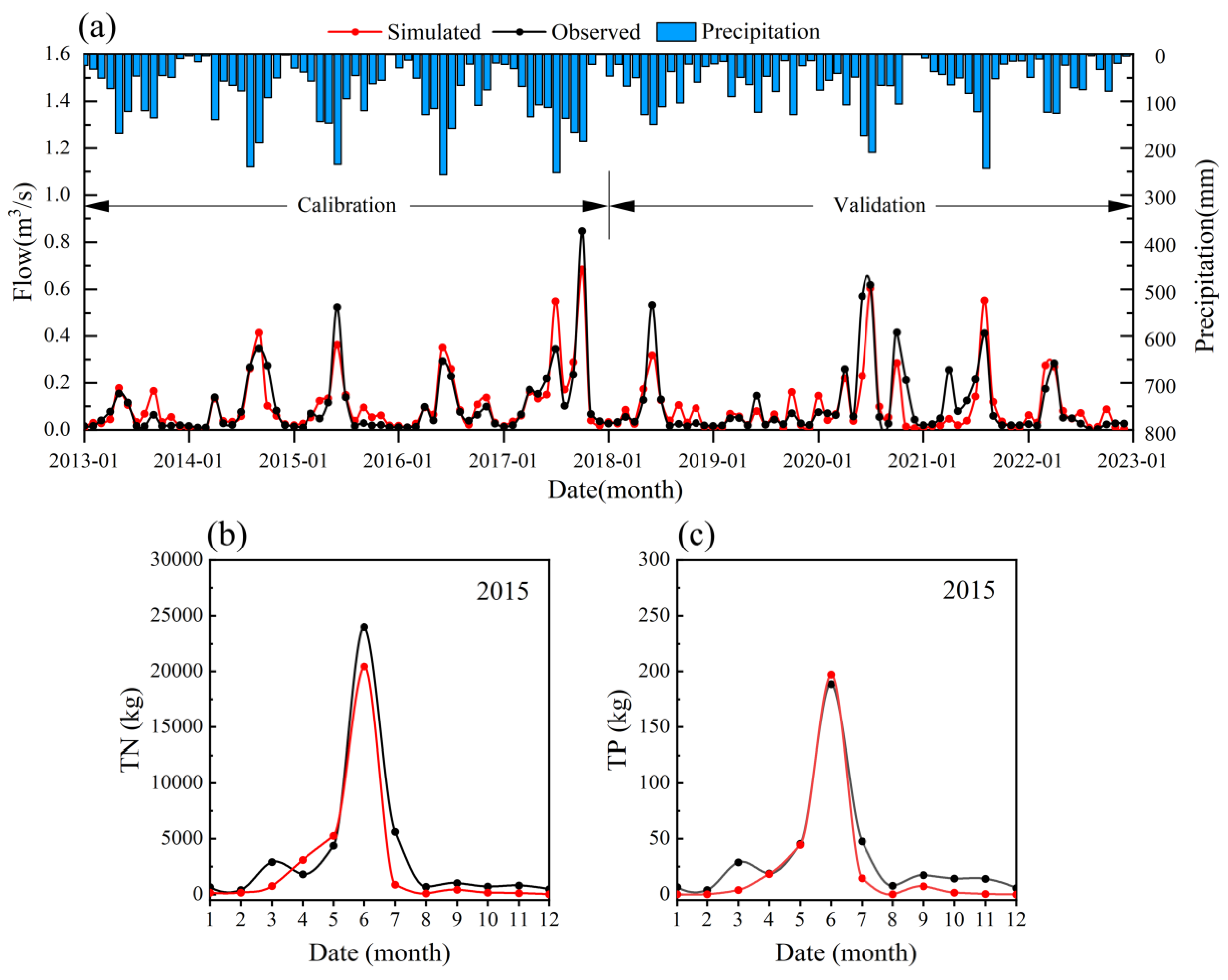
3.1. Model Performance in Simulating Flow and TN/TP Loads

Figure 2 displays the calibration and validation results for the flow and nutrient loads. According to monthly simulation results, the flow calibration period exhibited better performance compared with the validation period, with respective R² values of 0.85 and 0.70, NSE values of 0.85 and 0.7, and PBIAS values of 6.57% and −10.58%. Regarding monthly TN loads, the calibration results were satisfactory, with an R² of 0.94, an NSE of 0.91, and a PBIAS of −27.31%. Similarly, for TP loads, the calibration yielded favorable results, with an R² of 0.96, an NSE of 0.92, and a PBIAS of −27.64%. The evaluation criteria were suitably relaxed due to the higher uncertainties inherent in nutrient calibration, as recommended by Moriasi et al. [48]. Overall, the model evaluation indices indicate that the SWAT model demonstrates satisfactory performance in simulating flow and nutrient loads in the study area, rendering it suitable for investigating the effects of BMPs.

3.2. Distribution Characteristics and Drivers of TN/TP Loads in the Watershed

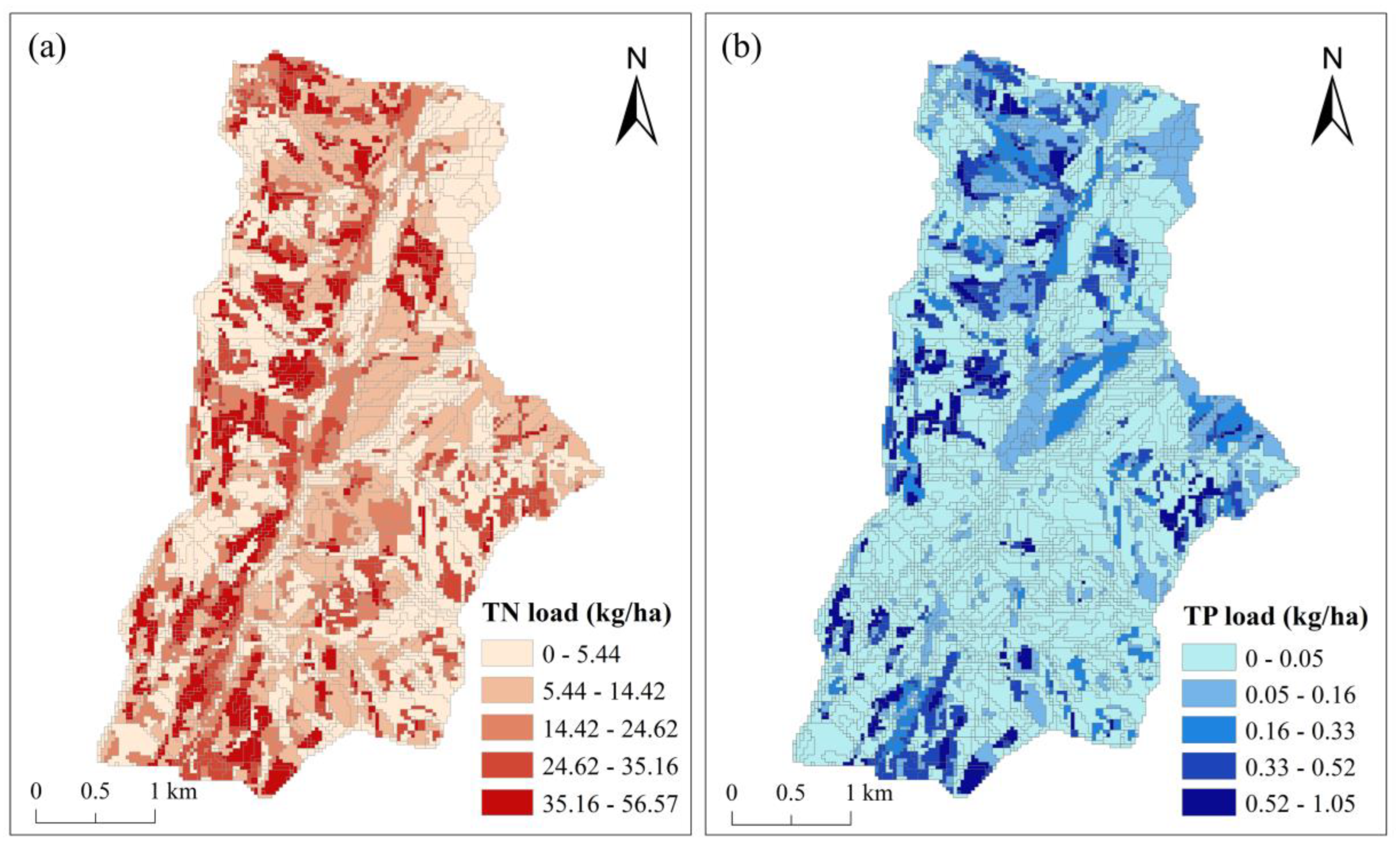
3.2.1. Distribution Characteristics

Figure 3 shows the multi-year average N and P loading intensities in the watershed. The spatial distribution of TN and TP loads exhibits significant variation across different locations, demonstrating clear spatial heterogeneity. The maximum TN output intensity in the watershed reaches 56.57 kg/ha, while the maximum TP loading intensity reaches 1.05 kg/ha. According to the statistical results presented in

Table 4. Summary of pollution loads on different land use types, kg/ha.

Land Use	Sloping Field	Orchard	Terrace	Paddy Field	Residential Area	Forest	Brush	Others	Entire Watershed
Area, ha	27.46	467.51	69.14	83.45	47.08	683.57	148.54	3.96	1530.71
TN loads	39.06	22.44	21.98	29.46	29.08	3.72	5.56	1.33	13.25
Organic N loads	35.12	13.78	17.04	24.63	26.93	3.69	5.5	1.31	9.96
Nitrate N loads	3.94	8.66	4.94	4.83	2.15	0.03	0.06	0.02	3.29
TP loads	0.32	0.18	0.11	0.34	0.07	0.03	0.06	0.05	0.11
Organic P loads	0.08	0.01	0.02	0.04	0.04	0.01	0.02	0.01	0.02
Sediment P loads	0.2	0.09	0.06	0.19	0.02	0.02	0.04	0.03	0.06
Dissolved P loads	0.04	0.07	0.02	0.11	0.02	0.01	0	0	0.03

, the average annual output intensities of TN and TP in the entire watershed are 13.25 kg/ha and 0.11 kg/ha, respectively. The average annual outputs of TN and TP in the watershed export amount to 20,281.91 kg and 168.38 kg, respectively. Concerning volume and intensity, TN pollution surpasses TP, indicating a more severe pollution level. Moreover, in terms of pollutant forms, organic nitrogen loss predominates in TN, while mineral phosphorus loss dominates in TP.

When comparing the nutrient loads across different land use types (Table 4), notable variations in nutrient loading intensities are evident for each type. The sloping field exhibited the highest TN loading intensity, with an average loading intensity of 39.06 kg/ha, which was 2.95 times higher than the watershed’s mean value. Conversely, the land use type with the highest TP loading intensity was the paddy field, displaying a loading intensity 3.09 times higher than the watershed’s mean value. In terms of the proportion of total load (Figure 4), Orchards demonstrated the highest percentages of TN and TP outputs, both exceeding 50% of the overall watershed loss. Forest TN and TP outputs accounted for 12.53% and 13.7%, respectively, despite covering the largest proportion of the watershed area at 44.66%. The residential area, constituting 3.08% of the watershed area, contributed 6.75% and 2.03% of the TN and TP output, respectively. Agricultural lands, including orchards, sloping fields, terraces, and paddy fields, accounted for 42.3% of the watershed area. However, they contributed 76.62% and 78.31% of the TN and TP output, respectively. These results indicate that agricultural lands significantly contribute to TN and TP loads.

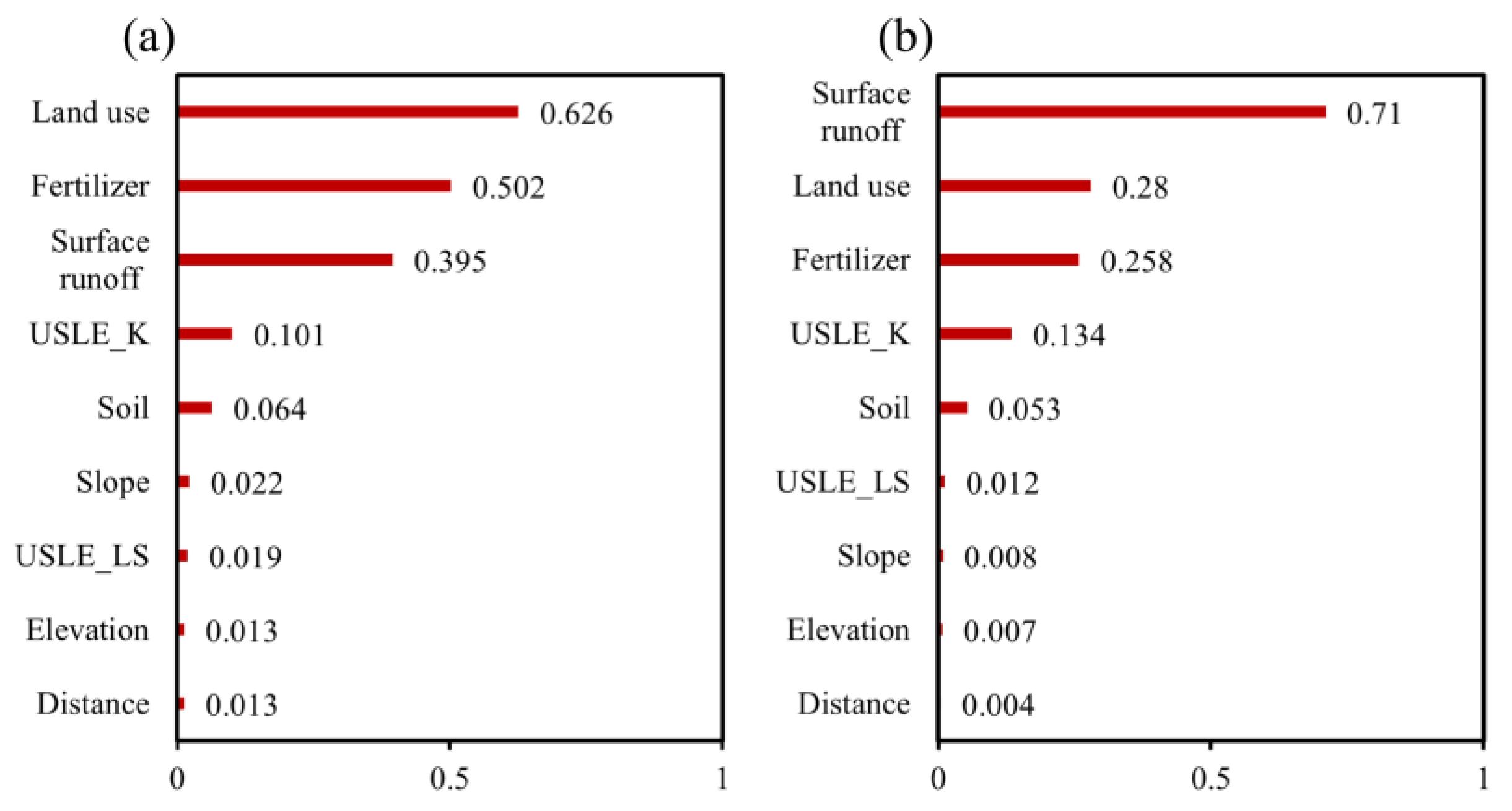
3.2.2. Driving Factors

The results of the factor detector are depicted in Figure 5. In determining the spatial distribution of TN, land use emerged as the most dominant driver (0.626), followed by nitrogen fertilizer application (0.502) and surface runoff (0.395). The relative importance of the other six influences ranged from 0 to 0.101. For TP, the top three dominant factors were surface runoff (0.71), land use (0.28), and phosphorus fertilizer application (0.258).

The findings of the interaction detection (Figure 6) reveal that the explanatory power of the interaction between land use and slope, soil type, surface runoff, USLE_LS, and USLE_K for TN loads exceeded 0.74. Notably, this explanatory power was significantly stronger compared with when these factors acted alone. Moreover, the explanatory power of surface runoff ∩ fertilizer application was found to be 0.743. As for TP, the q-values of surface runoff interacting with other factors ranged from 0.722 to 0.886, with the highest being the surface runoff ∩ fertilizer application. In summary, the loss of N and P loads in the watershed is influenced significantly by land use type and fertilizer application resulting from human activities, as well as surface runoff among natural factors. Conversely, the effects of six factors, namely, USLE_K, soil type, slope, USLE_LS, elevation, and distance from the water system, were observed to be relatively weak.

3.3. Efficiencies and Cost-Effectiveness of BMP Scenarios in Reducing NPS Pollution Loads

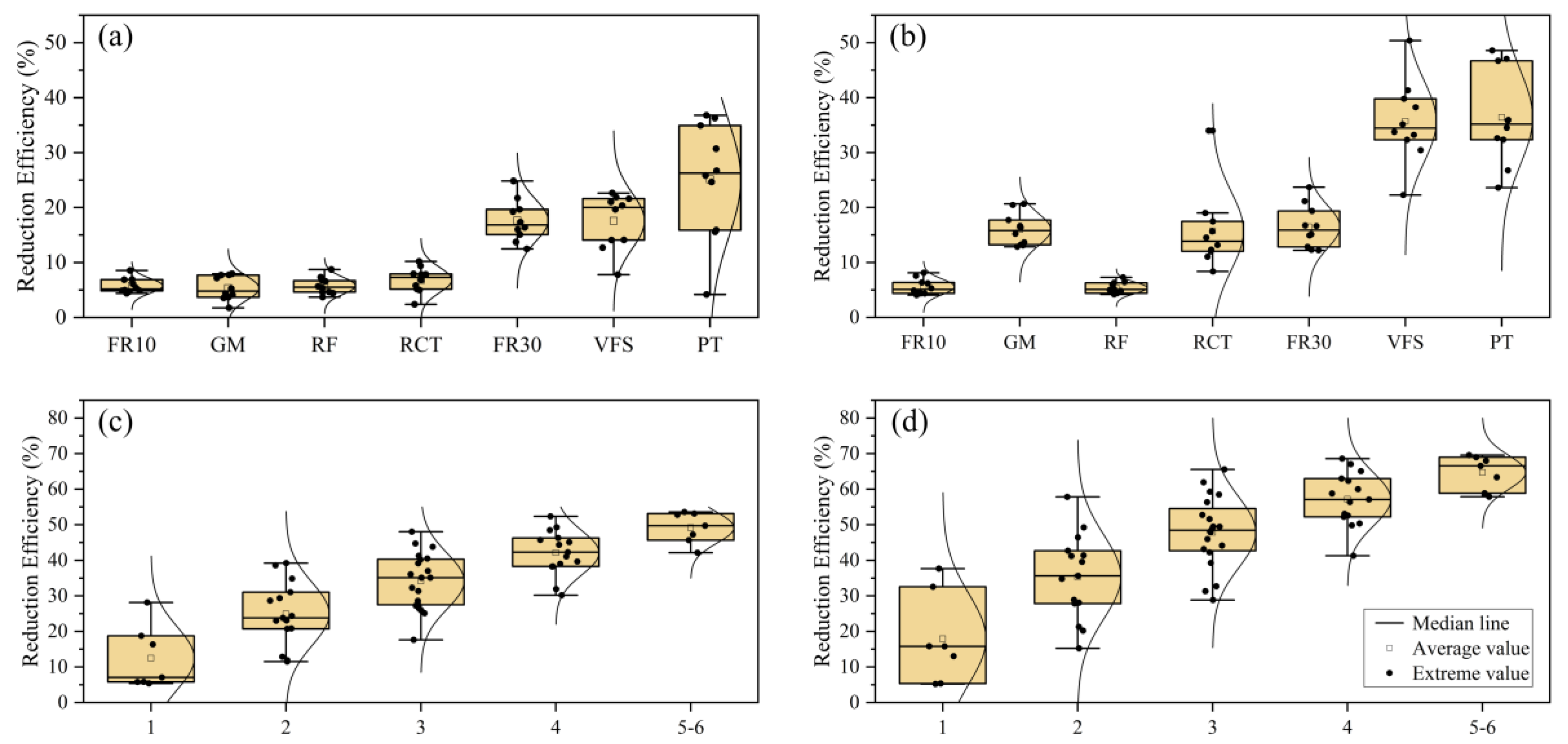
3.3.1. Efficiencies of BMP Scenarios

Figure 7a,b illustrate the reduction effects of individual BMPs over the simulation period.

Table 5. The reduction efficiency, cost, and comprehensive benefit value of individual BMPs.

Category	BMPs	Annual Costs, 104 CNY	TN Reduction Rate, %	TP Reduction Rate, %	Comprehensive Evaluation Indices
Structural measures	VFSs	2.1	18.75	32.53	0.47
	PTs	37.39	28.12	37.69	0.45
Non-structural measures	FR10	−12.3	5.38	5.35	0.31
	FR30	−36.91	16.34	15.77	0.51
	RCT	16.2	7.06	13.03	0.26
	GM	23.38	5.79	15.81	0.24
Landscape management measure	RF	10.19	5.81	5.21	0.24

presents the average annual reduction rates. The TN reduction rates for each measure in descending order are PTs (28.12%), VFSs (18.75%), FR30 (16.34%), RCT (7.06%), RF (5.81%), GM (5.79%), and FR10 (5.38%). As for the TP reductions, they are PTs (37.69%), VFSs (32.53%), GM (15.81%), FR30 (15.77%), RCT (13.03%), FR10 (5.35%), and RF (5.21%), in descending order. Among the individual BMPs, parallel terraces proved to be the most effective, followed by VFSs, both of which are structural BMPs. The reduction rates of PTs and VFSs exhibit high variability. Specifically, TN and TP reduction rates in PTs range from 4.17% to 36.79% and 23.61% to 48.58%, respectively. TN and TP reduction rates in VFSs range from 7.79% to 22.63% and 22.27% to 50.39%, respectively. Conversely, the reduction efficiency of FR10 and RF was lower, with an average reduction rate of less than 6% for both TN and TP. All BMPs, except for FR and RCT, were more effective in reducing TP than TN.

Figure 7c,d depict the variation in N and P reduction efficiency for different combinations. For TN loads, the average reduction rates for individual BMPs and combined BMPs with 2, 3, 4, and 5 measures were 12.46%, 24.91%, 34.61%, 42.15%, and 48.47%, respectively. The measures with the largest reduction rates in each group were PTs (28.12%), PT_FR30 (39.21%), VFS_PT_FR30 (48.05%), VFS_PT_RF_FR30 (49.3%), and VFS_PT_RF_RCT_FR30 (53.15%). For TP load, the mean reduction rates for the individual BMPs and the combined BMPs with 2, 3, 4, and 5 measures were 17.91%, 35.35%, 47.88%, 57.18%, and 64.04%, respectively. The measures with the highest reduction rates in each group were PTs (37.69%), VFS_PT (57.84%), VFS_PT_RCT (65.57%), VFS_PT_RCT_FR30 (68.58%), and VFS_PT_RCT_GM_FR30 (69.59%). Upon combining all six individual BMPs, the TN reduction rate was 53.6%, and the TP reduction rate was 69%. As the number of combinations increases, the average reduction rates of TN and TP gradually increase. However, there are also scenarios where BMPs with fewer measure combinations demonstrate reduction rates that approximate or even surpass the reduction effects achieved by BMPs with a higher number of combinations. For instance, PT_RCT demonstrated higher rates of TN and TP reduction, reaching 34.85% and 49.24%, respectively, compared with VFS_RCT_FR30, which achieved reductions of 31.32% for TN and 48.08% for TP. The combined implementation of BMPs proves to be less effective than simply summing up the pollutant reduction rates of individual BMPs. For instance, in the case of PT_FR30, the combination resulted in a reduction rate of 39.21%. However, the combined reduction rates for PTs and FR30 were 5.25% higher than that of PT_FR30. As the number of measure combinations increases, the range of reduction rate fluctuation gradually decreases and stabilizes.

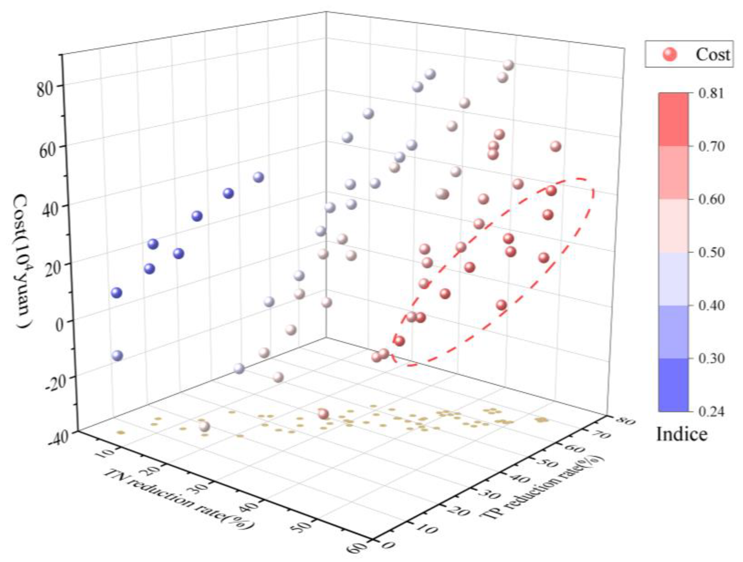
3.3.2. Cost-Effectiveness of BMP Scenarios

Table 5 presents the cost-effectiveness of different individual BMPs. In the simulation, FR30 is the most effective BMP with a rating of 0.51. Compared with other measures, FR30 offers cost-saving benefits. Additionally, VFSs and PTs also boast high ratings of 0.47 and 0.45, respectively—the benefit values of FR10, GM, RCT, and RF range from 0.24 to 0.31. The data in Figure 8 illustrate the distribution of all simulated scenarios. Among the combinations of BMPs with 2, 3, 4, and 5 measures, the BMPs with the highest combined environmental cost-benefit values are PT_FR30 (0.68), VFS_PT_FR30 (0.8), VFS_PT_RCT_FR30 (0.81), and VFS_PT_RF_RCT_FR30 (0.76). When all six individual BMPs are combined simultaneously, the benefit value is 0.69. In general, the evaluated values of these combined measures are significantly greater than FR30, indicating their superior cost-effectiveness in reducing NPS pollution in the watershed.

The top ten combinations, with the highest combined benefit values, are enclosed in the red dashed circle area of Figure 8, and their corresponding results are detailed in

Table 6. The top 10 BMPs in comprehensive benefits of environmental costs ranking.

Rank	BMPs in Series	Annual Costs, 104 CNY	TN Reduction Rate (%)	TP Reduction Rate (%)	Comprehensive Evaluation Indices
1	VFS_PT_RCT_FR30	18.79	52.37	68.58	0.81
2	VFS_PT_FR30	2.58	48.05	61.95	0.8
3	VFS_PT_RF_RCT_FR30	34.43	53.15	67.97	0.76
4	VFS_PT_RF_FR30	21.9	49.3	62.35	0.75
5	VFS_PT_RCT_GM_FR30	42.16	52.81	69.59	0.74
6	VFS_PT_GM_FR30	25.96	48.49	62.96	0.74
7	VFS_RCT_GM_FR30	4.77	39.68	57.11	0.71
8	PT_RCT_FR30	16.68	44.75	56.37	0.71
9	VFS_GM_FR30	−11.43	35.11	49.51	0.7
10	VFS_RF_RCT_FR30	−1.19	39.02	49.84	0.7

. Their comprehensive benefit values range from 0.7 to 0.81, with cost fluctuations spanning −114,300 to 421,600 CNY. The TN reduction rates range from 35.11% to 53.15%, and the TP reduction rates range from 49.51% to 69.59%. Notably, the scenario with the lowest cost ranks ninth, while the scenario with the highest TN reduction rate ranks third, and the scenario with the highest TP reduction rate ranks fifth. The most effective combination of measures is VFS_PT_RCT_FR30, which has a combined benefit value of 0.81 and a cost input of only 187,900 CNY, resulting in a 52.37% reduction in TN and a 68.58% reduction in TP. The combination ranked second is VFS_PT_FR30, which has a combined benefit value of 0.8 and reduces TN and TP by 48.05% and 61.95%, respectively, with a cost input of 25,800 CNY. VFS_PT_RCT_FR30 and VFS_PT_FR30 provide similar benefits. However, the TN and TP reduction rates of VFS_PT_RCT_FR30 are slightly higher than those of VFS_PT_FR30 (approximately 1.08 and 1.11 times, respectively). Despite this, the cost of VFS_PT_RCT_FR30 is 7.3 times higher than that of VFS_PT_FR30. The 9th and 10th ranked combinations showed negative cost values but were less effective in reducing N and P than the other combinations. They could be considered for use when funds are scarce. The top ten ranked combinations have measures appearing in the following order of frequency: FR30, PTs, VFSs, RCT, GM, and RF. This further illustrates the value of FR30, PTs, and VFSs for local applications.

4. Discussion

4.1. Analysis of Driving Factors for N and P Loss

The accurate comprehension of the output characteristics and primary drivers of N and P loads within watersheds is essential for the scientific development of pollution control strategies. The transport of N and P is influenced by various natural and anthropogenic factors [9], such as topography, precipitation, runoff, soils, land use, and fertilizer application. By employing the SWAT model in combination with Geodetector analysis, this study identified land use, fertilizer application, and surface runoff as the main factors driving spatial variations in N and P loads. The analysis revealed that land use predominantly dictates N distribution, whereas P distribution is primarily influenced by surface runoff due to its lower solubility compared with N. Furthermore, this study unveiled significant interaction effects among various factors. Notably, the combined effects of the runoff factor intersecting with land use and fertilizer application exhibited pronounced enhancement, amplifying their explanatory capacity. The study also revealed the significant enhancement effects of other factor interactions, indicating that, in actual processes, complex interactions between multiple factors collectively determine the spatial patterns of NPS pollution in watersheds [53].

The sources and transport processes of NPS pollution are highly dependent on hydrologic processes, with precipitation and runoff being the driving conditions for N and P transport [18,54,55]. Precipitation and surface runoff processes generally occur simultaneously, and the greater the precipitation and surface runoff, the more favorable the transport of sediment and nutrients [45]. Meteorological factors, such as precipitation, are assumed to be homogeneous within small watersheds; thus, the spatial exploration of their effects is neglected. However, runoff factors exhibit variability due to disparities in underlying surface characteristics, including slope, slope length, land use, soil properties, and other pertinent factors [21]. The underlying surface serves as the interface for nutrient transport, with surface runoff’s erosive and scouring forces escalating with increased slope and slope length, consequently amplifying nutrient transport capacity [56]. Research has shown significant differences in NPS loading between various soil types [57]. Soil types possess unique hydrological, biological, and background content traits, profoundly influencing soil erosion resistance, infiltration capacity, and flow production capacity [58]. Land use impacts the generation and transport of N and P loads, which is related to factors affecting vegetation cover and agricultural activities [59,60,61]. Wang et al. [19] found that the proportion of agricultural land use significantly affects nutrient loading. Vegetation cover affects the underlying surface characteristics, hydrological processes, and nutrient cycling, further influencing the storage and retention capacity of nutrients in different land use types [62]. Woodlands and shrubs can absorb and sequester nutrients to some extent, which helps mitigate the effects of pollution due to higher vegetation cover and less anthropogenic disturbance [7,63]. In contrast, agricultural land is plowed year-round, often exhibiting low vegetation cover or even bare ground. Crop growth relies on regular inputs of N and P fertilizers. Fertilizer application directly alters the initial soil nutrient content across various watershed regions. Elevated soil nutrient content increases the potential risk of agricultural NPS pollution formation through surface runoff and leaching loss [64]. Tan et al. [18] used the export coefficient model and Geodetector to assert that human activities have a dominant role in N and P output compared with natural factors. This statement implies that changes in regional N and P loads are strongly influenced by anthropogenic factors.

It is worth noting that the weak explanatory power of elevation observed in this study may be attributed to the influence of spatial scale effects on identifying influential factors [65,66]. Shen et al. [31] reported elevation as the predominant driver of spatial variance in the nutrient budget within the TGRA. The TGRA is 3832 times larger than the study watershed, with more drastic changes in elevation and a greater concentration of human activities at larger scales. Higher elevations typically exhibit greater vegetation cover and reduced human intervention, while lower elevations, particularly along rivers, are often urbanized or dedicated to agriculture [67]. In the studied watershed, despite the substantial range in elevation (201–1060 m), the impact of human activities does not vary significantly across different elevation bands.

In conclusion, exploring the potential drivers of N and P loads offers valuable insights into the characteristics of NPS load output within the watershed. This exploration can also aid in the selection of BMPs and delineation of implementation areas. The main objective is to reduce N and P loss from agricultural land, specifically orchards and cropland, within the watershed. This can be achieved by implementing changes in land use, reducing N and P inputs, controlling topography, and mitigating runoff. Additionally, a current limitation is that the nine drivers selected for this study may not fully account for the variations in N and P load outputs. Including additional potential drivers in future studies could enhance the explanatory power of N and P load outputs.

4.2. Analysis of Reduction Efficiency of Watershed BMPs

In different study areas, the effectiveness of identical measures can vary due to differences in climatic, geographical, and agro-economic conditions [33]. Leh et al. [34] observed a TN reduction of 1.2% to 4.9% from vegetated filter strips in an area with only 6% agricultural land. In contrast, Teshager et al. [68] modeled filter strips in a watershed with 78% agricultural land area and achieved reductions of approximately 50%. In our watershed, where agriculture covers 42.3% of the land area, filter strips can reduce TN by 7.79% to 22.63%. This highlights the significance of assessing and applying measures locally.

This study highlighted the notable reduction effects of structural measures such as terraces and vegetative filter strips, aligning with previous research by Sun et al. [32] and López-Ballesteros et al. [33]. However, even the most effective single measure, terracing, achieved a maximum reduction rate of only 28.12% for TN and 37.69% for TP. This underscores the challenge of attaining high reduction rates with individual measures alone, emphasizing the importance of integrating different measures [69,70,71]. Indeed, the study revealed that N and P reductions increased gradually with the combination of measures. It is essential to recognize that, while combined BMPs yielded better reduction effects than single measures, their impact was not purely additive due to interactions between the measures, as noted by Liu et al. [72]. When employing combined BMPs, pollutant concentrations diminish from upstream to downstream post-treatment with upstream BMPs. Consequently, downstream reduction efficiencies may be lower compared with their standalone implementation [73]. For instance, when reducing fertilizer use, the pollutant concentration in the vegetated filter strip treatment decreases, which, in turn, reduces the effectiveness of the filter strips in reducing pollutants [35].

Our study revealed that the reduction efficiency of TP caused by the implemented BMPs generally surpassed that of TN. This discrepancy can be attributed to the distinctive characteristics of elemental N and P in terms of form and transport transformation within water bodies, as well as the control mechanism of pollutants based on measures such as terracing, vegetative filter strips, and conservation tillage. Unlike P, N tends to be more soluble, with a portion lost through surface runoff, while another portion may leach into deeper soil layers, eventually reaching surface water through lateral flow or groundwater [74]. The mechanism of action of BMPs primarily relies on the physical interception or deposition of sediment, whereas treating dissolved matter in flow often requires biological and chemical reaction processes, which are less efficient and take longer to treat [75]. Consequently, controlling nitrogen proves to be more challenging than phosphorus due to these factors.

4.3. Analysis of Cost-Effectiveness of Watershed BMPs

To optimize BMPs, it is necessary to balance two interrelated and conflicting objectives: reducing pollution rates and minimizing input costs [76]. Since the Grain for Green project is an environmental measure strongly advocated by China’s ecological restoration project [77], our study simulated reforestation in line with national policy. However, considering the cost and pollution control perspective, the overall benefit of reforestation is not significant. Wu et al. [42] investigated the effect of reforestation on soil erosion control and found that it reached 32.16%. Nonetheless, the implementation cost was considered prohibitively high, resulting in poor overall benefits. Similarly, Sun et al. [32] excluded returning farmland to forest due to its high cost. Furthermore, this study shows that—due to the limited area of cultivable land meeting the requirements, which is only 40.77 ha, and the reduction rates of N and P being less than 6%—it is justifiable to rank the comprehensive benefit value at the lower end of the list.

This study’s comprehensive assessment of cost-effectiveness suggests that a rational mix of measures is necessary to achieve higher cost-effectiveness. It observes that combinations of BMPs with higher reduction rates often entail greater expenses, reflecting the inherent trade-off between pollution reduction rates and input costs [76]. The top-ranked solutions identified in this study offer valuable insights and references for decision-making amid varying economic and environmental constraints [78]. Decision-makers can select appropriate cost-effective options by making trade-offs based on specific economic costs and water quality objectives. Among the top ten combinations, vegetative filter strips, parallel terraces, and a 30% reduction in fertilizer were the most frequently recommended. The combination of all three BMPs ranked second. Vegetative filter strips are an economically inexpensive and effective method of preventing soil erosion and enhancing agricultural productivity. They have been recommended for implementation in many studies [34,35,79]. Given the mountainous terrain of the study area, the transformation of sloping land holds particular significance [80]. Moreover, FR30 emerged as the highest-rated individual BMP, offering both cost savings and substantial reductions in nutrient inputs from the source. Research indicates that agricultural fertilizer application in the TGRA is generally excessive [81,82]. Wang et al. [82] emphasized the importance of reducing N fertilizer input to mitigate net anthropogenic N input. Consequently, these findings suggest that combining the three measures above could be a suitable approach for implementation in the study area, as well as other watersheds within the TGRA.

5. Conclusions

In this study, we established a SWAT model for the Wangjiaqiao watershed to analyze the characteristics of nutrient load outputs. Utilizing a geographic detector, we identified the principal driving factors impacting the spatial distribution of nutrient loads within the watershed. Furthermore, we conducted simulations of various BMP scenarios and explored the feasibility of the watershed cost–benefit assessment framework through the entropy weight method. Our findings revealed spatial heterogeneity in N and P loads, with land use, fertilizer application, and surface runoff as primary drivers, exhibiting interactive enhancement effects. Structural BMPs demonstrated superior N and P reduction efficiency compared with individual measures. Combined BMPs showed greater reduction efficiency, but some combinations yielded less than the sum of individual measures. SWAT combined with the entropy weight method proved effective for selecting BMP schemes. The comprehensive benefits of combined BMPs were generally higher, highlighting the need for diverse strategies to address NPS pollution. The combination of vegetative filter strips, parallel terraces, and a 30% reduction in fertilizer application emerged as a promising approach, offering a balance between reduction benefits and economic feasibility, particularly for small watersheds within TGRA.

In conclusion, this study deepens our understanding of NPS pollution outputs and their underlying driving factors, providing valuable insights decision-makers can use to evaluate and optimize BMP strategies. In light of the limited available data, we exerted the utmost effort to calibrate the runoff and N/P load. Nevertheless, uncertainties stemming from model input data, structure, and parameters persist, indicating the necessity for further research in this domain. The predominant pollution sources in the study watershed are agricultural non-point sources, whereas contributions from residential activities and livestock farming are relatively minor and insignificantly impact these research findings; thus, they were appropriately disregarded. Due to the localized nature of optimization schemes and regional variations in BMP cost-effectiveness, future research should validate the reproducibility of our framework in basins with different scales and characteristics. Moreover, refining the BMP design around NPS pollution drivers, expanding the BMP application database, and developing corresponding simulation methods are crucial steps forward. Furthermore, there is a need to strengthen strategic research on managing stormwater runoff, improving land use structures, and enhancing agricultural production management at the basin scale to address the governance of NPS pollution issues.

References

1. Acuña-Alonso, C.; Fernandes, A.C.P.; Alvarez, X.; Valero, E.; Pacheco, F.A.L.; Varandas, S.D.P.; Terêncio, D.P.S.; Fernandes, L.F.S. Water security and watershed management assessed through the modelling of hydrology and ecological integrity: A study in the Galicia-Costa (NW Spain). Sci. Total Environ. 2021, 759, 143905. [Google Scholar] [CrossRef] [PubMed]
2. Casquin, A.; Gu, S.; Dupas, R.; Petitjean, P.; Gruau, G.; Durand, P. River network alteration of C-N-P dynamics in a mesoscale agricultural catchment. Sci. Total Environ. 2020, 749, 141551. [Google Scholar] [CrossRef] [PubMed]
3. Li, Y.Y.; Wang, H.; Deng, Y.Q.; Liang, D.F.; Li, Y.P.; Gu, Q.H. Applying water environment capacity to assess the non-point source pollution risks in watersheds. Water Res. 2023, 240, 120092. [Google Scholar] [CrossRef] [PubMed]
4. Conley, D.J.; Paerl, H.W.; Howarth, R.W.; Boesch, D.F.; Seitzinger, S.P.; Havens, K.E.; Lancelot, C.; Likens, G.E. Controlling Eutrophication: Nitrogen and Phosphorus. Science 2009, 323, 1014–1015. [Google Scholar] [CrossRef] [PubMed]
5. Liu, W.; Zhang, L.; Wu, H.L.; Wang, Y.F.; Zhang, Y.L.; Xu, J.Y.; Wei, D.Y.; Zhang, R.; Yu, Y.; Wu, D.S.; et al. Strategy for cost-effective BMPs of non-point source pollution in the small agricultural watershed of Poyang Lake: A case study of the Zhuxi River. Chemosphere 2023, 333, 138949. [Google Scholar] [CrossRef] [PubMed]
6. Wang, Y.; Feng, L.; Hou, X.J. Algal Blooms in Lakes in China Over the Past Two Decades: Patterns, Trends, and Drivers. Water Resour. Res. 2023, 59, e2022WR033340. [Google Scholar] [CrossRef]
7. Xue, B.L.; Zhang, H.W.; Wang, G.Q.; Sun, W.C. Evaluating the risks of spatial and temporal changes in nonpoint source pollution in a Chinese river basin. Sci. Total Environ. 2022, 807, 151726. [Google Scholar] [CrossRef] [PubMed]
8. Wang, R.J.; Wang, Q.B.; Dong, L.S.; Zhang, J.F. Cleaner agricultural production in drinking-water source areas for the control of non-point source pollution in China. J. Environ. Manag. 2021, 285, 112096. [Google Scholar] [CrossRef] [PubMed]
9. Wang, T.; Xiao, W.F.; Huang, Z.L.; Zeng, L.X. Interflow pattern govern nitrogen loss from tea orchard slopes in response to rainfall pattern in Three Gorges Reservoir Area. Agric. Water Manag. 2022, 269, 107684. [Google Scholar] [CrossRef]
10. Zhang, T.; Yang, Y.H.; Ni, J.P.; Xie, D.T. Construction of an integrated technology system for control agricultural non-point source pollution in the Three Gorges Reservoir Areas. Agric. Ecosyst. Environ. 2020, 295, 106919. [Google Scholar] [CrossRef]
11. Zhong, S.Q.; Chen, F.X.; Xie, D.T.; Shao, J.A.; Yong, Y.; Zhang, S.; Zhang, Q.W.; Wei, C.F.; Yang, Q.Y.; Ni, J.P. A three-dimensional and multi-source integrated technology system for controlling rural non-point source pollution in the Three Gorges Reservoir Area, China. J. Clean. Prod. 2020, 272, 122579. [Google Scholar] [CrossRef]
12. Wang, M.H.; Wang, Y.; Li, Y.; Liu, X.L.; Liu, J.; Wu, J.S. Natural and anthropogenic determinants of riverine phosphorus concentration and loading variability in subtropical agricultural catchments. Agric. Ecosyst. Environ. 2020, 287, 106713. [Google Scholar] [CrossRef]
13. Li, L.; Gou, M.M.; Wang, N.; Ma, W.; Xiao, W.F.; Liu, C.F.; La, L.M. Landscape configuration mediates hydrology and nonpoint source pollution under climate change and agricultural expansion. Ecol. Indic. 2021, 129, 107959. [Google Scholar] [CrossRef]
14. Xue, J.Y.; Wang, Q.R.; Zhang, M.H. A review of non-point source water pollution modeling for the urban-rural transitional areas of China: Research status and prospect. Sci. Total Environ. 2022, 826, 154146. [Google Scholar] [CrossRef] [PubMed]
15. Deng, X.J. Correlations between water quality and the structure and connectivity of the river network in the Southern Jiangsu Plain, Eastern China. Sci. Total Environ. 2019, 664, 583–594. [Google Scholar] [CrossRef] [PubMed]
16. Mao, Y.P.; Zhang, H.; Cheng, Y.H.; Zhao, J.W.; Huang, Z.W. The characteristics of nitrogen and phosphorus output in China’s highly urbanized Pearl River Delta region. J. Environ. Manag. 2023, 325, 116543. [Google Scholar] [CrossRef] [PubMed]
17. Wang, W.Z.; Chen, L.; Shen, Z.Y. Dynamic export coefficient model for evaluating the effects of environmental changes on non-point source pollution. Sci. Total Environ. 2020, 747, 141164. [Google Scholar] [CrossRef] [PubMed]
18. Tan, S.J.; Xie, D.T.; Ni, J.P.; Chen, L.; Ni, C.S.; Ye, W.; Zhao, G.Y.; Shao, J.A.; Chen, F.X. Output characteristics and driving factors of non-point source nitrogen (N) and phosphorus (P) in the Three Gorges reservoir area (TGRA) based on migration process: 1995-2020. Sci. Total Environ. 2023, 875, 162543. [Google Scholar] [CrossRef] [PubMed]
19. Wang, F.E.; Wang, Y.X.; Zhang, K.; Hu, M.; Weng, Q.; Zhang, H.C. Spatial heterogeneity modeling of water quality based on random forest regression and model interpretation. Environ. Res. 2021, 202, 111660. [Google Scholar] [CrossRef]
20. Feng, Q.Y.; Flanagan, D.C.; Engel, B.A.; Yang, L.; Chen, L.D. GeoAPEXOL, a web GIS interface for the Agricultural Policy Environmental eXtender (APEX) model enabling both field and small watershed simulation. Environ. Model. Softw. 2020, 123, 104569. [Google Scholar] [CrossRef]
21. Wang, S.H.; Wang, Y.Q.; Wang, Y.J.; Wang, Z. Assessment of influencing factors on non-point source pollution critical source areas in an agricultural watershed. Ecol. Indic. 2022, 141, 109084. [Google Scholar] [CrossRef]
22. Xie, H.; Dong, J.W.; Shen, Z.Y.; Chen, L.; Lai, X.J.; Qiu, J.L.; Wei, G.Y.; Peng, Y.X.; Chen, X.Q. Intra- and inter-event characteristics and controlling factors of agricultural nonpoint source pollution under different types of rainfall-runoff events. Catena 2019, 182, 104105. [Google Scholar] [CrossRef]
23. Guo, T.; Cibin, R.; Chaubey, I.; Gitau, M.; Arnold, J.G.; Srinivasan, R.; Kiniry, J.R.; Engel, B.A. Evaluation of bioenergy crop growth and the impacts of bioenergy crops on streamflow, tile drain flow and nutrient losses in an extensively tile-drained watershed using SWAT. Sci. Total Environ. 2018, 613, 724–735. [Google Scholar] [CrossRef]
24. Huang, J.; Liu, R.M.; Wang, Q.R.; Gao, X.; Han, Z.Y.; Gao, J.M.; Gao, H.; Zhang, S.B.; Wang, J.F.; Zhang, L.; et al. Climate factors affect N2O emissions by influencing the migration and transformation of nonpoint source nitrogen in an agricultural watershed. Water Res. 2022, 223, 119028. [Google Scholar] [CrossRef] [PubMed]
25. Luo, Z.Y.; Zhang, H.L.; Pang, J.Z.; Yang, J.; Li, M. Coupling of SWAT and EPIC Models to Investigate the Mutual Feedback Relationship between Vegetation and Soil Erosion, a Case Study in the Huangfuchuan Watershed, China. Forests 2023, 14, 844. [Google Scholar] [CrossRef]
26. Huang, J.J.; Lin, X.J.; Wang, J.H.; Wang, H. The precipitation driven correlation based mapping method (PCM) for identifying the critical source areas of non-point source pollution. J. Hydrol. 2015, 524, 100–110. [Google Scholar] [CrossRef]
27. Deng, J.; Zhou, Y.W.; Chu, L.; Wei, Y.J.; Li, Z.X.; Wang, T.W.; Dai, C.T. Spatiotemporal variations and determinants of stream nitrogen and phosphorus concentrations from a watershed in the Three Gorges Reservoir Area, China. Int. Soil Water Conserv. Res. 2023, 11, 507–517. [Google Scholar] [CrossRef]
28. Sun, S.Y.; Zhang, J.F.; Cai, C.J.; Cai, Z.Y.; Li, X.G.; Wang, R.J. Coupling of non-point source pollution and soil characteristics covered by Phyllostachys edulis stands in hilly water source area. J. Environ. Manag. 2020, 268, 110657. [Google Scholar] [CrossRef]
29. Yan, Z.Y.; Wang, Y.Q.; Wang, Z.; Zhang, C.R.; Wang, Y.J.; Li, Y.M. Spatiotemporal Analysis of Landscape Ecological Risk and Driving Factors: A Case Study in the Three Gorges Reservoir Area, China. Trans. ASABE 2023, 15, 4884. [Google Scholar] [CrossRef]
30. Fei, X.F.; Lou, Z.H.; Xiao, R.; Ren, Z.Q.; Lv, X.N. Contamination assessment and source apportionment of heavy metals in agricultural soil through the synthesis of PMF and GeogDetector models. Sci. Total Environ. 2020, 747, 141293. [Google Scholar] [CrossRef]
31. Shen, Z.L.; Zhang, W.S.; Peng, H.; Xu, G.H.; Chen, X.M.; Zhang, X.; Zhao, Y.X. Spatial characteristics of nutrient budget on town scale in the Three Gorges Reservoir area, China. Sci. Total Environ. 2022, 819, 152677. [Google Scholar] [CrossRef] [PubMed]
32. Sun, H.H.; Tian, Y.; Li, L.P.; Zhuang, Y.; Zhou, X.; Zhang, H.R.; Zhan, W.; Zuo, W.; Luan, C.Y.; Huang, K.M. Unraveling spatial patterns and source attribution of nutrient transport: Towards optimal best management practices in complex river basin. Sci. Total Environ. 2024, 906, 167686. [Google Scholar] [CrossRef] [PubMed]
33. López-Ballesteros, A.; Trolle, D.; Srinivasan, R.; Senent-Aparicio, J. Assessing the effectiveness of potential best management practices for science-informed decision support at the watershed scale: The case of the Mar Menor coastal lagoon, Spain. Sci. Total Environ. 2023, 859, 160144. [Google Scholar] [CrossRef] [PubMed]
34. Leh, M.D.K.; Sharpley, A.N.; Singh, G.; Matlock, M.D. Assessing the impact of the MRBI program in a data limited Arkansas watershed using the SWAT model. Agric. Water Manag. 2018, 202, 202–219. [Google Scholar] [CrossRef]
35. Lee, S.; McCarty, G.W.; Moglen, G.E.; Li, X.; Wallace, C.W. Assessing the effectiveness of riparian buffers for reducing organic nitrogen loads in the Coastal Plain of the Chesapeake Bay watershed using a watershed model. J. Hydrol. 2020, 585, 124779. [Google Scholar] [CrossRef]
36. Geng, R.Z.; Sharpley, A.N. A novel spatial optimization model for achieve the trad-offs placement of best management practices for agricultural non-point source pollution control at multi-spatial scales. J. Clean. Prod. 2019, 234, 1023–1032. [Google Scholar] [CrossRef]
37. Gassman, P.W.; Reyes, M.R.; Green, C.H.; Arnold, J.G. The soil and water assessment tool: Historical development, applications, and future research directions. Trans. ASABE 2007, 50, 1211–1250. [Google Scholar] [CrossRef]
38. Wallace, C.W.; Flanagan, D.C.; Engel, B.A. Quantifying the effects of conservation practice implementation on predicted runoff and chemical losses under climate change. Agric. Water Manag. 2017, 186, 51–65. [Google Scholar] [CrossRef]
39. Risal, A.; Parajuli, P.B. Evaluation of the Impact of Best Management Practices on Streamflow, Sediment and Nutrient Yield at Field and Watershed Scales. Water Resour. Manag. 2022, 36, 1093–1105. [Google Scholar] [CrossRef]
40. Yuan, Y.P.; Koropeckyj-Cox, L. SWAT model application for evaluating agricultural conservation practice effectiveness in reducing phosphorous loss from the Western Lake Erie Basin. J. Environ. Manag. 2022, 302, 114000. [Google Scholar] [CrossRef]
41. Liu, Y.Z.; Guo, T.; Wang, R.Y.; Engel, B.A.; Flanagan, D.C.; Li, S.Y.; Pijanowski, B.C.; Collingsworth, P.D.; Lee, J.G.; Wallace, C.W. A SWAT-based optimization tool for obtaining cost-effective strategies for agricultural conservation practice implementation at watershed scales. Sci. Total Environ. 2019, 691, 685–696. [Google Scholar] [CrossRef] [PubMed]
42. Wu, L.; Liu, X.; Chen, J.L.; Li, J.F.; Yu, Y.; Ma, X.Y. Efficiency assessment of best management practices in sediment reduction by investigating cost-effective tradeoffs. Agric. Water Manag. 2022, 265, 107546. [Google Scholar] [CrossRef]
43. Cheng, W.J.; Xi, H.Y.; Sindikubwabo, C.; Si, J.H.; Zhao, C.G.; Yu, T.F.; Li, A.L.; Wu, T.R. Ecosystem health assessment of desert nature reserve with entropy weight and fuzzy mathematics methods: A case study of Badain Jaran Desert. Ecol. Indic. 2020, 119, 106843. [Google Scholar] [CrossRef]
44. Xiang, R.; Wang, L.J.; Li, H.; Tian, Z.B.; Zheng, B.H. Water quality variation in tributaries of the Three Gorges Reservoir from 2000 to 2015. Water Res. 2021, 195, 116993. [Google Scholar] [CrossRef] [PubMed]
45. Zhou, Y.W.; Li, Z.X.; Wang, T.W.; Wang, J.; Deng, J.; Du, Y.N.; Dai, C.T.; Zhang, X.M.; Zhao, S.J. Divergent hydrological responses to intensive production under different rainfall regimes: Evidence from long-term field observations. J. Hydrol. 2023, 617, 128918. [Google Scholar] [CrossRef]
46. Garosi, Y.; Sheklabadi, M.; Conoscenti, C.; Pourghasemi, H.R.; Van Oost, K. Assessing the performance of GIS-based machine learning models with different accuracy measures for determining susceptibility to gully erosion. Sci. Total Environ. 2019, 664, 1117–1132. [Google Scholar] [CrossRef] [PubMed]
47. Ding, W.L.; Xia, J.; She, D.X.; Zhang, X.Y.; Chen, T.; Huang, S.; Zheng, H.S.Y. Assessing multivariate effect of best management practices on non-point source pollution management using the coupled Copula-SWAT model. Ecol. Indic. 2023, 153, 110393. [Google Scholar] [CrossRef]
48. Moriasi, D.N.; Arnold, J.G.; Van Liew, M.W.; Bingner, R.L.; Harmel, R.D.; Veith, T.L. Model evaluation guidelines for systematic quantification of accuracy in watershed simulations. Trans. ASABE 2007, 50, 885–900. [Google Scholar] [CrossRef]
49. Woo, S.Y.; Kim, S.J.; Lee, J.W.; Kim, S.H.; Kim, Y.W. Evaluating the impact of interbasin water transfer on water quality in the recipient river basin with SWAT. Sci. Total Environ. 2021, 776, 145984. [Google Scholar] [CrossRef]
50. Wang, J.F.; Hu, Y. Environmental health risk detection with GeogDetector. Environ. Model. Softw. 2012, 33, 114–115. [Google Scholar] [CrossRef]
51. Alnahit, A.O.; Mishra, A.K.; Khan, A.A. Stream water quality prediction using boosted regression tree and random forest models. Stoch. Environ. Res. Risk Assess. 2022, 36, 2661–2680. [Google Scholar] [CrossRef]
52. Arabi, M.; Frankenberger, J.R.; Enge, B.A.; Arnold, J.G. Representation of agricultural conservation practices with SWAT. Hydrol. Process. 2008, 22, 3042–3055. [Google Scholar] [CrossRef]
53. Shi, J.H.; Jin, R.; Zhu, W.H. Quantification of Effects of Natural Geographical Factors and Landscape Patterns on Non-point Source Pollution in Watershed Based on Geodetector: Burhatong River Basin, Northeast China as An Example. Chin. Geogr. Sci. 2022, 32, 707–723. [Google Scholar] [CrossRef]
54. Li, T.Y.; Zhang, Y.; He, B.H.; Wu, X.Y.; Du, Y.N. Nitrate loss by runoff in response to rainfall amount category and different combinations of fertilization and cultivation in sloping croplands. Agric. Water Manag. 2022, 273, 107916. [Google Scholar] [CrossRef]
55. Zhou, Y.; Li, S.Y.; Huang, Y.R.; Chen, M.H.; Huang, L. Modeling of rainfall induced phosphorus transport from soil to runoff with consideration of phosphorus-sediment interactions. J. Hydrol. 2022, 609, 127732. [Google Scholar] [CrossRef]
56. Xin, Y.; Liu, G.; Xie, Y.; Gao, Y.; Liu, B.Y.; Shen, B. Effects of soil conservation practices on soil losses from slope farmland in northeastern China using runoff plot data. Catena 2019, 174, 417–424. [Google Scholar] [CrossRef]
57. Shen, Z.Y.; Chen, L.; Ding, X.W.; Hong, Q.; Liu, R.M. Long-term variation (1960-2003) and causal factors of non-point-source nitrogen and phosphorus in the upper reach of the Yangtze River. J. Hazard. Mater. 2013, 252, 45–56. [Google Scholar] [CrossRef] [PubMed]
58. Liu, R.M.; Zhang, P.P.; Wang, X.J.; Chen, Y.X.; Shen, Z.Y. Assessment of effects of best management practices on agricultural non-point source pollution in Xiangxi River watershed. Agric. Water Manag. 2013, 117, 9–18. [Google Scholar] [CrossRef]
59. Wang, K.; Wang, P.X.; Zhang, R.D.; Lin, Z.B. Determination of spatiotemporal characteristics of agricultural non-point source pollution of river basins using the dynamic time warping distance. J. Hydrol. 2020, 583, 124303. [Google Scholar] [CrossRef]
60. Shen, Z.Y.; Qiu, J.L.; Hong, Q.; Chen, L. Simulation of spatial and temporal distributions of non-point source pollution load in the Three Gorges Reservoir Region. Sci. Total Environ. 2014, 493, 138–146. [Google Scholar] [CrossRef]
61. Srinivas, R.; Singh, A.P.; Dhadse, K.; Garg, C. An evidence based integrated watershed modelling system to assess the impact of non-point source pollution in the riverine ecosystem. J. Clean. Prod. 2020, 246, 118963. [Google Scholar] [CrossRef]
62. Bu, H.M.; Zhang, Y.; Meng, W.; Song, X.F. Effects of land-use patterns on in-stream nitrogen in a highly-polluted river basin in Northeast China. Sci. Total Environ. 2016, 553, 232–242. [Google Scholar] [CrossRef] [PubMed]
63. Fang, S.B.; Deitch, M.J.; Gebremicael, T.G.; Angelini, C.; Ortals, C.J. Identifying critical source areas of non-point source pollution to enhance water quality: Integrated SWAT modeling and multi-variable statistical analysis to reveal key variables and thresholds. Water Res. 2024, 253, 121286. [Google Scholar] [CrossRef] [PubMed]
64. Yang, X.Y.; Liu, Q.; Fu, G.T.; He, Y.; Luo, X.Z.; Zheng, Z. Spatiotemporal patterns and source attribution of nitrogen load in a river basin with complex pollution sources. Water Res. 2016, 94, 187–199. [Google Scholar] [CrossRef] [PubMed]
65. Chen, L.; Chen, S.B.; Li, S.; Shen, Z.Y. Temporal and spatial scaling effects of parameter sensitivity in relation to non-point source pollution simulation. J. Hydrol. 2019, 571, 36–49. [Google Scholar] [CrossRef]
66. Zhu, Y.X.; Chen, L.; Wang, K.; Wang, W.Z.; Wang, C.C.; Shen, Z.Y. Evaluating the spatial scaling effect of baseflow and baseflow nonpoint source pollution in a nested watershed. J. Hydrol. 2019, 579, 124221. [Google Scholar] [CrossRef]
67. Huang, C.B.; Huang, X.; Peng, C.H.; Zhou, Z.X.; Teng, M.J.; Wang, P.C. Land use/cover change in the Three Gorges Reservoir area, China: Reconciling the land use conflicts between development and protection. Catena 2019, 175, 388–399. [Google Scholar] [CrossRef]
68. Teshager, A.D.; Gassman, P.W.; Secchi, S.; Schoof, J.T. Simulation of targeted pollutant-mitigation-strategies to reduce nitrate and sediment hotspots in agricultural watershed. Sci. Total Environ. 2017, 607, 1188–1200. [Google Scholar] [CrossRef]
69. Mtibaa, S.; Hotta, N.; Irie, M. Analysis of the efficacy and cost-effectiveness of best management practices for controlling sediment yield: A case study of the Joumine watershed, Tunisia. Sci. Total Environ. 2018, 616, 1–16. [Google Scholar] [CrossRef]
70. Uniyal, B.; Jha, M.K.; Verma, A.K.; Anebagilu, P.K. Identification of critical areas and evaluation of best management practices using SWAT for sustainable watershed management. Sci. Total Environ. 2020, 744, 140737. [Google Scholar] [CrossRef]
71. Zhang, Z.S.; Montas, H.; Shirmohammadi, A.; Leisnham, P.; Negahban-Azar, M. Effectiveness of BMP plans in different land covers, with random, targeted, and optimized allocation. Sci. Total Environ. 2023, 892, 164428. [Google Scholar] [CrossRef] [PubMed]
72. Liu, Y.Z.; Wang, R.Y.; Guo, T.; Engel, B.A.; Flanagan, D.C.; Lee, J.G.; Li, S.Y.; Pijanowski, B.C.; Collingsworth, P.D.; Wallace, C.W. Evaluating efficiencies and cost-effectiveness of best management practices in improving agricultural water quality using integrated SWAT and cost evaluation tool. J. Hydrol. 2019, 577, 123965. [Google Scholar] [CrossRef]
73. Liu, Y.Z.; Bralts, V.F.; Engel, B.A. Evaluating the effectiveness of management practices on hydrology and water quality at watershed scale with a rainfall-runoff model. Sci. Total Environ. 2015, 511, 298–308. [Google Scholar] [CrossRef] [PubMed]
74. Zhang, Y.Y.; Xia, J.; Shao, Q.X.; Zhai, X.Y. Water quantity and quality simulation by improved SWAT in highly regulated Huai River Basin of China. Stoch. Environ. Res. Risk Assess. 2013, 27, 11–27. [Google Scholar] [CrossRef]
75. Kalcic, M.M.; Kirchhoff, C.; Bosch, N.; Muenich, R.L.; Murray, M.; Gardner, J.G.; Scavia, D. Engaging Stakeholders To Define Feasible and Desirable Agricultural Conservation in Western Lake Erie Watersheds. Environ. Sci. Technol. 2016, 50, 8135–8145. [Google Scholar] [CrossRef] [PubMed]
76. Dong, F.F.; Li, J.C.; Dai, C.; Niu, J.; Chen, Y.; Huang, J.C.; Liu, Y. Understanding robustness in multiscale nutrient abatement: Probabilistic simulation-optimization using Bayesian network emulators. J. Clean. Prod. 2022, 378, 134394. [Google Scholar] [CrossRef]
77. Li, W.Q.; Zinda, J.A.; Zhang, Z.M. Does the “Returning Farmland to Forest Program” Drive Community-Level Changes in Landscape Patterns in China? Forests 2019, 10, 933. [Google Scholar] [CrossRef]
78. Yang, L.; Pang, S.J.; Wang, X.Y.; Du, Y.; Huang, J.Y.; Melching, C.S. Optimal allocation of best management practices based on receiving water capacity constraints. Agric. Water Manag. 2021, 258, 107179. [Google Scholar] [CrossRef]
79. Zhang, X.; Li, P.; Bin Li, Z.; Yu, G.Q. Effects of grass strips distribution on soil erosion and its optimal configuration on hillslopes. Catena 2024, 238, 107882. [Google Scholar] [CrossRef]
80. Wang, N.A.; Luo, J.; He, S.Q.; Li, T.X.; Zhao, Y.H.; Zhang, X.Z.; Wang, Y.D.; Huang, H.G.; Yu, H.Y.; Ye, D.H.; et al. Characterizing the rill erosion process from eroded morphology and sediment connectivity on purple soil slope with upslope earthen dike terraces. Sci. Total Environ. 2023, 860, 160486. [Google Scholar] [CrossRef]
81. Han, J.X.; Xin, Z.H.; Han, F.; Xu, B.; Wang, L.F.; Zhang, C.; Zheng, Y. Source contribution analysis of nutrient pollution in a P-rich watershed: Implications for integrated water quality management. Environ. Pollut. 2021, 279, 116885. [Google Scholar] [CrossRef] [PubMed]
82. Wang, Z.; Wang, Y.Q.; Ding, X.K.; Wang, Y.J.; Yan, Z.Y.; Wang, S.H. Evaluation of net anthropogenic nitrogen inputs in the Three Gorges Reservoir Area. Ecol. Indic. 2022, 139, 108922. [Google Scholar] [CrossRef]
Figure 1. Location of (a) the Three Gorges Reservoir Area, (b) Zigui County, and (c) the Wangjiaqiao watershed.
Land 13 00742 g001
Figure 2. Observed and simulated monthly (a) streamflow, (b) TN, and (c) TP loads at the outlet. TN/TP has only a calibration period due to a lack of sufficient data for validation.
Land 13 00742 g002
Figure 3. Spatial distribution of multi-year average (a) TN load and (b) TP load at HRU level.
Land 13 00742 g003
Figure 4. The proportion of area, TN load, and TP load to the total in different land use types.
Land 13 00742 g004
Figure 5. The q-values of potential drivers of (a) TN and (b) TP.
Land 13 00742 g005
Figure 6. The q-values for the interaction of potential drivers of (a) TN and (b) TP.
Land 13 00742 g006
Figure 7. (a) TN and (b) TP reduction efficiency of individual BMPs; (c) TN and (d) TP reduction efficiency of BMPs with a different number of combinations.
Land 13 00742 g007
Figure 8. TN/TP reduction rates, costs, and comprehensive evaluation indices for all BMPs.
Land 13 00742 g008