Abstract
This paper presents an updated wilderness quality map, WQI 2.0, for Europe, which extends the existing map (WQI 1.0) to include non-EU states in Eastern Europe. The analysis utilizes the Google Earth Engine (GEE) cloud platform and incorporates contemporary datasets to assess wilderness quality across the continent. WQI 2.0 is compared to the previous version from the EU Wilderness register and global data from the WCS Human Influence Index (HII). Results indicate a high level of consistency between the versions, validating the robustness of the approach and the value of up-to-date datasets. WQI 2.0 serves as a valuable tool for developing a coordinated European policy on wilderness protection, encompassing both EU and non-EU states. By identifying areas outside current protected boundaries, the map helps to identify regions at risk of degradation and loss, due to resource exploitation. While small changes are seen between WQI 1.0 and WQI 2.0, expanding the coverage over the whole of continental Europe provides a foundation for the longer-term monitoring and evaluation of conservation targets. The findings contribute to meeting international commitments, such as the COP15 Kunming–Montreal Agreement and CBD targets, by highlighting the importance of preserving intact wilderness areas and increasing protected areas through restoration and rewilding efforts. Future iterations, such as WQI 3.0+, can track trends and potential threats to wilderness areas, while also identifying opportunities for ecosystem recovery through restoration and rewilding. To ensure comprehensive coverage, there is a need to update the existing Wilderness Register 1.0 and expand its scope to include non-EU states. This can be facilitated through collaboration with national WQI mapping programs, building on the experiences of countries such as Scotland, France, Iceland, and Germany, which have well-established national mapping initiatives. Overall, WQI 2.0 and the proposed updates provide valuable tools for informed decision-making in wilderness conservation and restoration efforts across Europe.
1. Introduction
Understanding and mapping wilderness is vital for contemporary conservation and land management efforts. Wilderness, characterised by its untouched or minimally modified state, plays a crucial role in preserving biodiversity, maintaining ecological processes, and providing essential ecosystem services. It serves as a refuge for rare and endangered species, promotes genetic diversity, and supports natural processes. Moreover, wilderness areas offer invaluable opportunities for scientific research, education, recreation, and spiritual renewal [1,2].
By delineating and assessing wilderness areas, we can effectively prioritize conservation efforts, monitor changes over time, and develop sustainable land use policies. Early efforts to map wilderness began in the 1980s by R.G. Lesslie and S.G. Taylor, alongside the development of computer-based methodologies [3,4]. Since then, advancements in computing technologies and data accessibility have revolutionised research in this field, enabling more comprehensive studies. However, the escalating human impact on wilderness highlights the urgency for both research and political action. This underscores the significance of this field of research now more than ever, as political decisions and strategies must be well informed and grounded in reliable spatial data.
In February 2009, the European Parliament passed the Resolution on Wilderness in Europe (2008/2210(INI)). It was adopted with 538 votes in favour and only 19 against, thus representing a massive cross-party endorsement and a strong popular mandate for action. The resolution called on the European Commission to do the following:
- Develop a clear definition of wilderness in Europe.
- Mandate the European Environment Agency to map existing wilderness areas in Europe.
- Undertake a study on the values and benefits of wilderness.
- Develop a wider EU wilderness strategy.
- Stimulate the development of new wilderness areas through restoration.
- Promote the values of wilderness together with NGOs and local communities.
The Resolution was followed in May with a conference organised by Wild Europe in Prague, under the Czech Presidency, on Wilderness and Large Natural Habitat Areas, at which the present parties developed a series of policy recommendations for the protection and restoration of Europe’s wilderness and wild areas. This was subsequently written up by Wild Europe in the “Poseltví from Prague” (Message from Prague) as an agenda for action on Europe’s wild areas. Key action points were to develop a review of wilderness in Europe; establish and agree a definition for wilderness, relevant to the European setting; and compile a register of legally protected wilderness areas. A review of the status and conservation of wild land in Europe was completed in November 2010 [5] and a set of guidelines on wilderness in Natura 2000, containing a unifying definition of wilderness in Europe, followed early in 2013 [6]. This guidance document established the following formal definition for wilderness in Europe:
“A wilderness is an area governed by natural processes. It is composed of native habitats and species, and large enough for the effective ecological functioning of natural processes. It is unmodified or only slightly modified and without intrusive or extractive human activity, settlements, infrastructure or visual disturbance”. (p. 2) [6].
The definition was scripted by Wild Europe and agreed by the European Commission as the basis for the 2013 guidelines and subsequent Wilderness Register. The definition includes the following four basic and fundamental qualities of wilderness: (a) naturalness, (b) undisturbedness, (c) undeveloped nature, and (d) scale; an overarching and changing variable, which, by definition, is central to the wilderness concept. A rigorous and coherent map showing of the distribution and quality of wilderness areas is, therefore, required to underpin developing policy on wilderness in Europe and, in a broader context, to address the catastrophic declines in wilderness areas worldwide [7].
Early mapping work by Carver [8] in the EEA, “Europe’s Ecological Backbone” report, and presented at the Prague conference, was ultimately used as a core component of the EU Wilderness Register [9], in which a database of designated wilderness areas, a spatial index of wilderness quality, and an analysis of protected vs. unprotected wilderness areas is presented for the EU27 and partner states. This wilderness quality index (WQI) is now 10 years old and, thus, requires updating, using current data. The 2013 index (WQI 1.0) is also restricted to the EU27 states and would benefit from expansion to cover all of continental Europe, including non-EU states and Russia, west of the Ural Mountains.
This paper updates and extends the existing WQI 1.0 to include current data and Eastern European states including Armenia, Azerbaijan, Belarus, Georgia, Moldova, Russia (European part), and Ukraine. We adapt the original WQI model and apply this approach using the Google Earth Engine (GEE) to map a new updated wilderness index (WQI 2.0) across the whole of continental Europe.
2. Materials and Methods
In general, the analysis described here follows the logic used to produce the first EU WQI 1.0 for the Wilderness Register [9], where the wilderness quality index was calculated as a weighted linear combination of the following three main factors: namely, (1) naturalness of landcover, (2) remoteness from access, and (3) remoteness from the population. Each of these factors is constructed in multiple data processing steps, as described below.
2.1. Naturalness of Landcover
This layer is based on the reclassified ESA WorldCover 10 m landcover [10] for the year 2020. This dataset was selected because of its pan-European coverage, fine resolution, and recent date of production. The original WQI 1.0 was built on a more detailed Copernicus CORINE landcover, but unfortunately this dataset does not cover non-EU countries in Eastern Europe.
During the reclassification procedure, original landcover classes were substituted with naturalness scores (see Table 1) ranging from 1 to 10, corresponding to the lowest and highest naturalness values, respectively.

Table 1.
Original and reclassified values of landcover.
Forests were assigned the score of nine because large areas of European forest cover either have an artificial origin (i.e., are commercial plantation forestry) and/or are intensively managed and modified [11]. Here, we followed the approach in Kuiters et al. [9] from the original EU Wilderness Register (and Index) report. There are a broad range of ‘managed’ forests from intensive, single non-native species (e.g., Sitka spruce) planted in rows and blocks with rotational clear felling/thinning to continuous cover forestry with native species and selective feeling/firewood collection. While the non-native commercial forestry operations could be given a lower weight, unified data on such operations across Europe are not available. This is better addressed in local level mapping.
However, the naturalness scores of selected forested areas were increased to 10 in those places that overlap with the primary forests areas identified in the “European primary forest database v2.0” [12].
Pixels corresponding to grasslands were altered by a scaled grazing intensity layer, produced as an equally weighted linear combination of cattle, sheep, and horse densities from the FAOs Gridded Livestock of the World v. 4 (GLW) rasters (DA models [13,14,15]). A threshold of 1000 animals/km2 was applied to the GLW data values, rescaled between 0 and 1, and inverted such that in the final grazing intensity product, pixels with values close to ‘0’ represent the highest grazing intensity and pixels close to 1 represent the lowest. “Grassland” pixels in the reclassified landcover were multiplied by the grazing intensity values, so that grasslands where grazing intensity is high were penalised and values where grazing intensity is close to zero maintained a high naturalness score.
All cells corresponding to water were masked and other landcover classes were eventually rescaled to a uniform unit scale (between 0 and 1).
2.2. Remoteness from Mechanised Access
Remoteness from mechanised access was calculated as a cost–distance surface, measured as the minimum time required to travel from a source cell (normally a road) to another location. The starting point for this analysis was a friction surface built by reclassifying the same ESA WorldCover 10 m landcover [10] into times needed to cross 1 metre of terrain at a normal walking speed. GEE [16] algorithms automatically convert these values into the time needed to cross a raster cell or pixel at a given resolution. Here, we assume that the speed of crossing herbaceous wetlands and terrain with sparse vegetation such as moss or lichens is equal to 2 km/h and for forests and shrublands this is equal to 3 km/h. For all other landcover classes, the speed is equal to 5 km/h. Main rivers and open water were treated as uncrossable barriers and were masked from the friction surface by setting null values to corresponding pixels, except in those places where barriers are crossed by roads (e.g., bridges).
As the speed of travel also depends on topography, the friction surface was augmented by applying penalties calculated according to Scarf’s formula [17,18], which is based on Naismith’s rule [19]. For this, ascending rate was calculated as a function of the slope (tangent times pixel resolution), which was derived from the Multi-Error-Removed Improved-Terrain Digital Elevation Model (MERIT DEM) [20].
We used trunk, primary, secondary, tertiary, and unclassified roads from the OpenStreetMap database [21] as the source from which cost–distance is calculated, with the maximum distance for cost calculations set to 20 km to speed up calculation. Eventually, a threshold of 3 h was applied to the resulting cost surface, assuming that the average human can travel up to 15 km at an average speed of 5 km/h, so the initial distance limit of cost–distance calculations has no effect on the final results. The raster was then rescaled and unmasked with the value of ‘1’ for areas that are further than the 3 h thresholds. Null values in the raster caused by rivers (uncrossable barriers) in the final products were substituted with median values obtained from a 3 × 3 pixels focal filter.
Cost–distance rasters were created for each road class separately (i.e., cost–distance to trunk–primary, secondary, tertiary, and unclassified roads) and then combined as a weighted sum with weights set as 0.4, 0.3, 0.2, and 0.1, respectively.
2.3. Remoteness from Population
Remoteness from population was also calculated as a cost–distance surface and the initial steps of producing the friction surface are the same as with distance from access. The principal difference here is that the initial friction surface was augmented with the road network to take travel times into account. Pixels that overlapped with the trunk–primary, secondary, and tertiary–unclassified roads were assigned time costs corresponding to speeds of 110, 90, and 50 km/h, respectively. The road network was added in a way that masked rivers are overlaid with roads pixels, effectively forming bridges that can be used by the cost–distance algorithm to cross water barriers.
Settlement boundaries from the OSM database were used as a source for cost distance calculations and were augmented with residential roads from the same database. This was necessary because not all settlements, especially those in eastern Europe, are covered by the OSM database as polygons with the tags ‘residential’ or ‘place’. Including residential roads, therefore, decreases the possibility of missing many such settlements. An alternative source of settlements was also tested, namely those pixels with a value of ‘50’ (built-up areas) from the ESA landcover. However, visual inspections indicated some presence of classification noise (i.e., false settlements) which may influence the results of cost calculations.
Distance from the population raster was further augmented with two additional data sources, as follows: monthly averaged and corrected VIIRS night light data [22], using a threshold of 30 nanoWatts/cm2/sr; and CIESIN Gridded Population of the World density data [23], using a threshold set at 1000 people/km2, following the thresholds used in [24]. Both rasters were then rescaled to unit scale, inverted, and multiplied with each other. The combined product was added in an equally weighted sum with the initial cost distance to the population raster. This procedure is similar to the weighting of a cost raster, as places with high night light emissions and population densities (e.g., highly populated places like cities) eventually obtained much lower values than remote and sparsely populated areas in the final ‘remoteness from population’ raster.
2.4. Wilderness Index Calculations
The final wilderness quality index map (WQI v2.0) was calculated as a linear combination of the following three mentioned intermediate products: the naturalness of landcover, remoteness from access, and remoteness from the population, with equal weights (Figure 1). The final product is masked to the area of interest, the European continent, and exported.
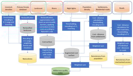
Figure 1.
Wilderness analysis flowchart.
2.5. Data Sources and Software
The analysis was performed entirely on the GEE cloud platform [16] with many data sources (see Table 2) directly imported from the GEE collections. Some layers were manually imported as additional assets. Among these are OSM layers of roads, rivers, and settlements, as well as primary forests from the Sabatini et al. [12] dataset and FAO GLW data [13,14,15].
Table 2.
Key data sources used for wilderness analysis.
2.6. Statistical Analysis
The correlation between WQI v2.0, WCS Human Modification Map, and WQI v1.0 from the first wilderness register were tested using two approaches. Pairwise Pearson’s correlation coefficients were calculated from 20,000 random pixel samples in the overlapping extent of map pairs. For this cor.test() function in R was used. Also, correlations of raster pairs were calculated using a reduceNeighborhood() reducer and moving window with Person’s correlation on GEE (kernel size 2.5), which produced rasters showing local levels of correlation and related p-values.
3. Results
The produced wilderness map reveals distinct longitudinal and latitudinal gradients in the distribution of wilderness across Europe. As depicted in Figure 2 and Figure 3, there is a discernible increase in the average wilderness quality indices towards the northern and eastern regions of the continent. Additionally, a pronounced correlation is observed between wilderness quality and altitude, with higher values predominantly found in mountainous areas.
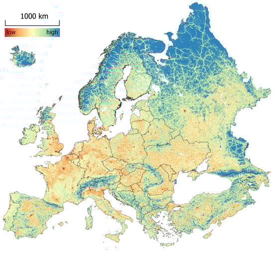
Figure 2.
Wilderness quality index map WQI 2.0.
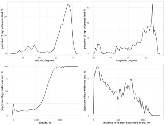
Figure 3.
Proportion of available land with a wilderness index value of ≥0.95 in gradients of latitude, longitude, altitude, and distance to oceans or seas across Europe.
The analysis of the wilderness quality index reveals notable variations in relation to different protected area designations. Specifically, the index tends to be higher on lands that fall under the IUCN categories of 1a, 1b, and 2 (strict nature reserves, wilderness areas, and national parks, respectively), indicating a stronger presence of wilderness in these protected areas (Figure 4). Furthermore, sites included in the Emerald network, which focuses on the conservation of the most valuable and threatened habitats and species in some non-EU countries, also exhibit higher wilderness quality index values. Surprisingly, the wilderness quality index does not demonstrate a significant increase in NATURA 2000 sites, which are designated for the protection of habitats and species of European importance within the EU.
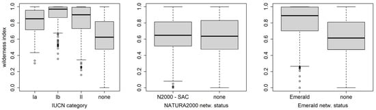
Figure 4.
Comparison of wilderness index distribution across different types of protected areas in Europe.
The distribution of wild lands across countries follows a similar pattern to the longitudinal, latitudinal, and altitudinal gradients described earlier. Mountainous and northern countries (Table 3) tend to exhibit a higher proportion of wild lands, reflecting the influence of rugged terrain, colder climates, and historical land use patterns.
Table 3.
European countries by the proportion of their territory with a high wilderness index (≥0.95).
Overall, WQI 2.0 correlates well with its predecessor, WQI 1.0 from the Wilderness register (r = 0.76, p < 0.001), and with the recent WCS human modification index map (resampled, inverted, and rescaled to unit scale; r = 0.70, p < 0.001). The other two mentioned datasets correlate strongly with each other (r = 0.81, p < 0.001).
When examined spatially, the utilisation of local correlations between different versions of WQI 1.0 and WCS HMI reveals an overall strong positive correlation (values close to ‘1’ or green on the colour version of the map; see Figure 5 and Figure 6) across the western half of Europe. Notably, strong negative correlations (values close to ‘−1’, or red on the colour version of the map) are generally absent, indicating that the different versions of WQI maps do not contradict each other. It is not possible to compare WQI 1.0 and 2.0 in Eastern Europe, as the first map did not cover these areas. However, comparisons with WCS HII in the eastern half of the continent generally align with the observations noted above.
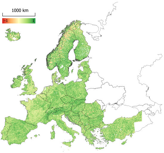
Figure 5.
Focal correlation between the current wilderness map (WQI 2.0) and the map used in the original wilderness register (WQI 1.0). Note that the original wilderness register map covers only the western half of Europe.
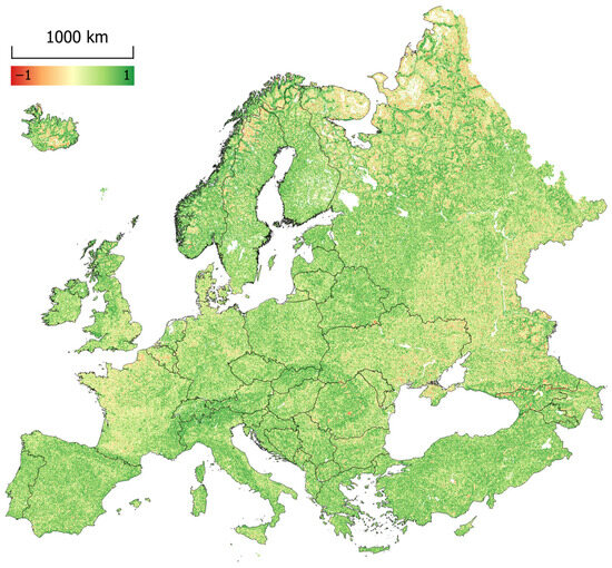
Figure 6.
Focal correlation between the current wilderness map (WQI 2.0) and the inverted and scaled WCS Human Influence Index map.
Difference maps between WQI 1.0 and 2.0 indicate results close to zero across most of Europe, without any discernible geographical trends (refer to Figure 7). While some clusters of similar values may form, no discernible trends are observed in altitudinal, longitudinal, or latitudinal directions.
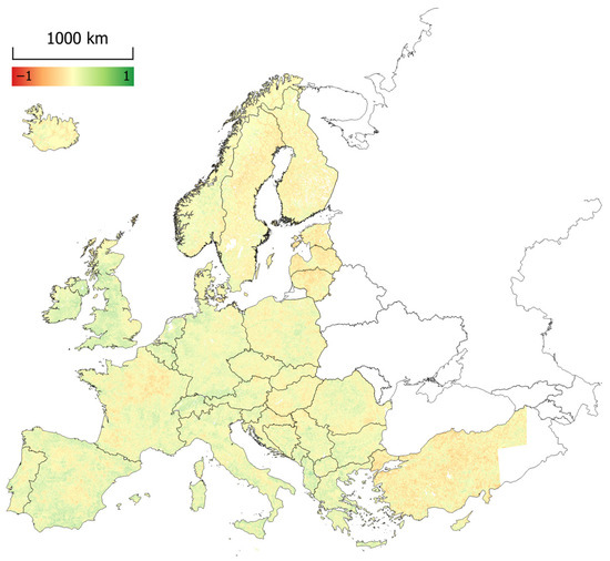
Figure 7.
Difference between the current wilderness map (WQI 2.0) and the map used in the original wilderness register (WQI 1.0). Note that the original wilderness register map covers only the western half of Europe.
When compared to WCS HII (Figure 8), minimal differences are observed in mountainous areas and the far northeast, both of which are regarded as regions of high wilderness in both maps. Conversely, the most significant differences are observed in steppe or lowland regions. However, overall, the disparity between these two maps does not exhibit striking values.
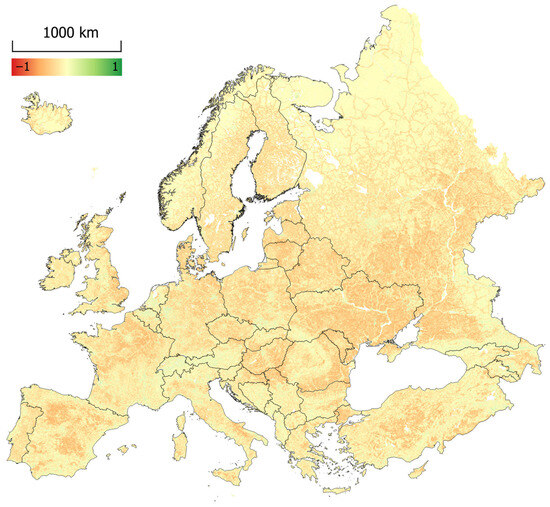
Figure 8.
Difference between the current wilderness map (WQI 2.0) and the inverted and scaled WCS Human Influence Index map.
4. Discussion
The patterns seen in WQI 2.0 (Figure 2) closely mirror those seen in the original WQI 1.0 map. This is demonstrated by the close correlation between the WQI values in Figure 5 and the general lack of absolute difference between the two versions, where these coincide across the Western European states (Figure 7). This is repeated in comparison with the WCS Human Influence Index (HII), as shown in Figure 6 and Figure 8, though WQI 2.0 tends towards over-estimation when compared the global scale mapping of WCS HII. Perhaps unsurprisingly, all maps reveal a strong altitudinal and latitudinal trend in wilderness quality, with higher values found in higher altitude/latitude areas. This can be attributed to broadscale patterns in land suitability for agriculture and settlement.
More local variations that diverge from this general trend across Europe and within countries can be seen in some locations such as estuarine and lowland marsh/heath, as well as dry steppe environments. Again, these tend to reflect the suitability of land for agriculture, settlement, and other human use. Localised impacts from mining and oil/gas exploitation may be discerned in some remote areas, together with connecting transport routes.
Table 3 ranks the countries by the proportion of their territory with a high wilderness index value (≥0.95). Iceland is at the top of this list, with 37% of the country falling into the high wilderness index category. This confirms the existing work on mapping wilderness in Iceland, which, based on WQI 1.0, shows 43% of Europe’s top 1% wildest areas to be in Iceland [26]. Other Scandinavian countries are also present in the top 20 including Norway, Sweden, and Finland. Eastern European states not included in WQI 1.0 also feature prominently, including Georgia, Azerbaijan, and Armenia, due to their combined mountainous nature and significant proportion of dry steppe landscapes, while Russia is prominent due to its vast size and significant areas of northern boreal forest and tundra. Most of the other countries appearing in this list do so because of significant areas of mountainous terrain, even including the apparent outliers of Liechtenstein and Andorra.
Geographical scale and resolution are both significant issues, as regards the data used and analyses performed in this paper and elsewhere. This is especially the case regarding global versus regional/national data quality and the uncertainty that generates, modelling assumptions made therein, and the increased sophistication of spatial models aimed at the actual measurement of the human impact on wilderness quality, rather than relying on proxies. For example, consider measures of remoteness and accessibility. At a global scale, these are mapped using the proxy of straight-line distance from the nearest point of mechanised access, while at regional and local levels, remoteness can be measured as time taken to walk from the nearest road or other access point using anisotropic models that take terrain, land cover, barrier features, and other factors into account [27]. These potentially affect ecosystem service delivery to human populations. Such benefits are dependent on distance, in that nearer wilderness areas (‘urban proximate’) may deliver greater ecosystem service value by direct association than wilderness areas that are more remote from human populations. This very much depends, however, on what service is used and its delivery mechanism. For example, benefits from wilderness watersheds can be delivered to urban populations many miles downstream from water quality and supply, flood water retention, and erosion control, while benefits to coast populations from barrier dune and mangrove ecosystems are highly localised [28].
The spatial scale also affects spatial data availability and accuracy. Patterns of wilderness quality can change markedly, depending on the scale of the observation and the resolution of the data used. Maps developed using high integrity local data, fine spatial resolutions, and sophisticated modelling tools can reveal patterns that are simply not available to global mapping projects.
Several national and local level WQI mapping programmes exist for selected European countries and areas. For example, national maps exist for Scotland [29], Iceland [26], Germany [30], Denmark [31], France [32], Switzerland [33], etc. These have been able to incorporate national datasets and more locally nuanced models taking local culture and landscape into account and, as such, could serve as tools for calibrating the accuracy and reliability of the regional level models presented here. This highlights the potential for a programme of national wilderness maps across Europe and the need for local adaptations, taking national variations in data, geography, and culture into account, as well as the consideration of transboundary cooperation to avoid and account for inevitable edge effects across national land borders.
Potential uses of WQI 2.0 and a new Wilderness Register 2.0 include the ability to identify wilderness areas that remain outside the current protected area boundaries and, thus, are potentially at risk from degradation and loss, resulting from resource exploitation such as forestry and mining. The Wilderness Register 1.0 was able to demonstrate that large areas of Europe, particularly in northern latitudes and selected mountain areas, remain unprotected despite possessing all the necessary attributes of wilderness as defined by the EU Wilderness Guidelines [9]. Such areas could prove to be a useful focus for meeting EU and national commitments under the recent COP15 Kunming–Montreal Agreement on the 30 × 30 vision and relevant CBD targets. In particular, Target 3 states that we should “Ensure and enable that by 2030 at least 30 per cent of terrestrial and inland water areas, and of marine and coastal areas, especially areas of particular importance for biodiversity and ecosystem functions and services, are effectively conserved and managed through ecologically representative, well-connected and equitably governed systems of protected areas…”, while the protection and restoration of wilderness has been placed first in a list of 21 action targets of the Convention on Biological Diversity’s (CBD’s) post-2020 global biodiversity framework (GBF).
5. Conclusions
In this paper, we present an updated wilderness quality map, WQI 2.0, for Europe that extends the existing map, WQI 1.0, to include the non-EU states in Eastern Europe, using GEE and contemporary datasets. We compare the new map with the earlier version from the EU Wilderness register and global data from WCS HII. While differences can be seen, these are generally small and demonstrate the robustness of the approach and the value of up-to-date datasets and regional focus of the mapping programme. WQI 2.0 represents a valuable addition to the existing map and provides a basis for developing a more coordinated European policy on wilderness protection across the EU and non-EU states over the next 10 years. We propose that the mapping should be accompanied by updates to the Wilderness Register and include Eastern European countries as far east as the Ural Mountains.
The geographic extent of potential wilderness in the EU, and thus Europe, has yet to be finalised because the definition of “strict protection” proposed by the EU Biodiversity Strategy for 30% of the 30% (i.e., ~10% of the total area) of the EU’s terrestrial and marine areas targeted for protection has yet to determined. However, Wild Europe is proposing to make complete non-intervention the default for strict protection, with exceptions only where interventionist conservation measures are necessary for protecting endangered species or secondary habitats, such as old growth and primary forest [34].
Thus, it should be clear that identifying the remaining intact wilderness areas that could be preserved, as well as the proportion of land and sea areas where such areas should be increased via ecological restoration and rewilding is a priority goal in addressing the linked climate and biodiversity crises. Repeat mapping over the coming decades in WQI 3.0+ could further be used to identify trends and possible threats to the remaining wilderness areas, as well as to identify opportunities where restoration and rewilding could help ecosystems and biodiversity recover. There is a clear need for updates to the existing Wilderness Register 1.0 and to expand this to include non-EU states across continental Europe. This could be assisted by a network of national WQI mapping programmes building on existing experience and work in key countries such as Scotland, France, Iceland, and Germany, where national mapping programmes are well underway.
Author Contributions
Conceptualisation, S.C.; methodology, S.C. and I.S.; software, I.S.; validation, S.C. and I.S.; formal analysis, I.S.; writing—original draft preparation, S.C. and I.S.; writing—review and editing, S.C. and I.S.; visualisation, I.S.; supervision, S.C. and I.S.; funding acquisition, S.C. All authors have read and agreed to the published version of the manuscript.
Funding
This research was funded by Frankfurt Zoological Society and the University of Leeds.
Data Availability Statement
The raw data supporting the conclusions of this article will be made available by the authors on request.
Acknowledgments
We are grateful to the OpenStreetMap (OSM) contributors, whose invaluable input was essential to the success of this study. We would also like to express our appreciation to the authors of the original datasets used in this study. The availability and accessibility of datasets such as the EU Wilderness Register, WCS Human Influence Index, primary forests data, and FAO GLW data were instrumental in enabling the accurate assessment of wilderness quality across the continent. Furthermore, we would like to acknowledge the developers and researchers behind the Google Earth Engine (GEE) cloud platform which provided a powerful and efficient computational environment for processing and analysing the vast amounts of geospatial data involved in this study. We are grateful to support from Wild Europe and Frankfurt Zoological Society for supporting this work.
Conflicts of Interest
The authors declare no conflicts of interest.
References
- Pérez-Hämmerle, K.V.; Moon, K.; Venegas-Li, R.; Maxwell, S.; Simmonds, J.S.; Venter, O.; Garnett, S.T.; Possingham, H.P.; Watson, J.E. Wilderness forms and their implications for global environmental policy and conservation. Conserv. Biol. 2022, 36, e13875. [Google Scholar] [CrossRef] [PubMed]
- Convention on Biological Diversity. First Draft of the Post-2020 Global Biodiversity Framework-2017. Available online: https://www.cbd.int/doc/c/abb5/591f/2e46096d3f0330b08ce87a45/wg2020-03-03-en.pdf (accessed on 22 July 2023).
- Lesslie, R.G.; Taylor, S.G. The wilderness continuum concept and its implications for Australian wilderness preservation policy. Biol. Conserv. 1985, 32, 309–333. [Google Scholar] [CrossRef]
- Lesslie, R.G.; Mackey, B.G.; Preece, K.M. A computer-based method of wilderness evaluation. Environ. Conserv. 1988, 15, 225–232. [Google Scholar] [CrossRef]
- Fisher, M.; Carver, S.; Kun, Z.; McMorran, R.; Arrell, K.; Mitchell, G.; Kun, S. Review of status and conservation of wild land in Europe. Rep. Wildland Res. Inst. Univ. Leedsuk 2010, 148, 131. Available online: http://www.self-willed-land.org.uk/rep_res/0109251.pdf (accessed on 19 January 2023).
- Wild Europe. A Working Definition of European Wilderness and Wild Areas. 2013. Available online: https://www.europarc.org/wp-content/uploads/2015/05/a-working-definition-of-european-wilderness-and-wild-areas.pdf (accessed on 15 September 2023).
- Watson, J.E.; Shanahan, D.F.; Di Marco, M.; Allan, J.; Laurance, W.F.; Sanderson, E.W.; Mackey, B.; Venter, O. Catastrophic declines in wilderness areas undermine global environment targets. Curr. Biol. 2016, 26, 2929–2934. [Google Scholar] [CrossRef] [PubMed]
- EEA [European Environment Agency]. EEA Report No. 6/2010. Europe’s Ecological Backbone: Recognising the True Value of our Mountains. Available online: https://www.eea.europa.eu/publications/europes-ecological-backbone (accessed on 19 January 2023).
- Kuiters, A.T.; van Eupen, M.; Carver, S.; Fisher, M.; Kun, Z.; Vancura, V. Wilderness Register and Indicator for Europe Final Report; EEA Contract No 0703072011610387 SERB3; European Environment Agency: Copenhagen, Denmark, 2013. [Google Scholar]
- Zanaga, D.; Van De Kerchove, R.; Daems, D.; De Keersmaecker, W.; Brockmann, C.; Kirches, G.; Wevers, J.; Cartus, O.; Santoro, M.; Fritz, S.; et al. ESA WorldCover 10 m 2021 v200. Available online: https://doi.org/10.5281/zenodo.7254221 (accessed on 1 February 2023).
- Forest Europe: State of Europe’s Forests 2020. Available online: https://wilderness-society.org/european-wilderness-definition (accessed on 20 August 2023).
- Sabatini, F.M.; Bluhm, H.; Kun, Z.; Aksenov, D.; Atauri, J.A.; Buchwald, E.; Burrascano, S.; Cateau, E.; Diku, A.; Duarte, I.M.; et al. European primary forest database v2.0. Sci. Data 2021, 8, 220. [Google Scholar] [CrossRef] [PubMed]
- Gilbert, M.; Cinardi, G.; Da Re, D.; Wint, W.G.R.; Wisser, D.; Robinson, T.P. Global Cattle Distribution in 2015 (5 Minutes of Arc), Harvard Dataverse, V1, 2022. Available online: https://doi.org/10.7910/DVN/LHBICE (accessed on 9 September 2023).
- Gilbert, M.; Cinardi, G.; Da Re, D.; Wint, W.G.R.; Wisser, D.; Robinson, T.P. Global HORSES Distribution in 2015 (5 Minutes of Arc), Harvard Dataverse, V1, 2022. Available online: https://doi.org/10.7910/DVN/JJGCTX (accessed on 9 September 2023).
- Gilbert, M.; Cinardi, G.; Da Re, D.; Wint, W.G.R.; Wisser, D.; Robinson, T.P. Global Sheep Distribution in 2015 (5 Minutes of Arc), Harvard Dataverse, V1, 2022. Available online: https://doi.org/10.7910/DVN/VZOYHM (accessed on 9 September 2023).
- Gorelick, N.; Hancher, M.; Dixon, M.; Ilyushchenko, S.; Thau, D.; Moore, R. Google Earth Engine: Planetary-scale geospatial analysis for everyone. Remote Sens. Environ. 2017, 202, 18–27. [Google Scholar] [CrossRef]
- Scarf, P. Route choice in mountain navigation, Naismith’s rule, and the equivalence of distance and climb. J. Sports Sci. 2007, 25, 719–726. [Google Scholar] [CrossRef] [PubMed]
- Kay, A. Pace and critical gradient for hill runners: An analysis of race records. J. Quant. Anal. Sports 2012, 8, 1–17. [Google Scholar] [CrossRef][Green Version]
- Naismith, W.W. Cruach Ardran, Stobinian, and Ben More. Scott. Mt. Club J. 1892, 2, 136. [Google Scholar]
- Yamazaki, D.; Ikeshima, D.; Tawatari, R.; Yamaguchi, T.; O’Loughlin, F.; Neal, J.C.; Sampson, C.C.; Kanae, S.; Bates, P.D. A high accuracy map of global terrain elevations. Geophys. Res. Lett. 2017, 44, 5844–5853. [Google Scholar] [CrossRef]
- OpenStreetMap Contributors. OpenStreetMap Database from Geofabrick.de Exports. OpenStreetMap Foundation: Cambridge, UK. Available online: https://www.geofabrik.de (accessed on 7 November 2023).
- Mills, S.; Weiss, S.; Liang, C. VIIRS day/night band (DNB) stray light characterization and correction. Earth Obs. Syst. XVIII 2013, 8866, 549–566. [Google Scholar] [CrossRef]
- Center for International Earth Science Information Network—CIESIN—Columbia University. Gridded Population of the World, Version 4 (GPWv4): Population Density; Revision 11; NASA Socioeconomic Data and Applications Center (SEDAC): Palisades, NY, USA, 2018; Available online: https://doi.org/10.7927/H49C6VHW (accessed on 30 January 2023).
- Ekim, B.; Dong, Z.; Rashkovetsky, D.; Schmitt, M. The naturalness index for the identification of natural areas on regional scale. Int. J. Appl. Earth Obs. Geoinf. 2021, 105, 102622. [Google Scholar] [CrossRef]
- Vogt, J.; Rimaviciute, E.; de Jager, A. CCM2 River and Catchment Database for Europe Version 2.1 Release Notes. European Commission-Joint Research Centre–Institute for Environment and Sustainability, 2008, Ispra, Italy, 5pp. Available online: https://ccm.jrc.ec.europa.eu/documents/JVogt_etal_CCM21.pdf (accessed on 30 January 2023).
- Carver, S.; Konráðsdóttir, S.; Guðmundsson, S.; Carver, B.; Kenyon, O. New Approaches to Modelling Wilderness Quality in Iceland. Land 2008, 12, 446. [Google Scholar] [CrossRef]
- Carver, S. Mapping wilderness and opportunities for rewilding. In Routledge Handbook of Rewilding; Hawkins, S., Convery, I., Carver, S., Beyers, R., Eds.; Taylor & Francis: Oxfordshire, UK, 2022. [Google Scholar] [CrossRef]
- Fisher, B.; Turner, R.K.; Morling, P. Defining and classifying ecosystem services for decision making. Ecol. Econ. 2009, 68, 643–653. [Google Scholar] [CrossRef]
- Carver, S.; Comber, A.; McMorran, R.; Nutter, S. A GIS model for mapping spatial patterns and distribution of wild land in Scotland. Landsc. Urban Plan. 2012, 104, 395–409. [Google Scholar] [CrossRef]
- Schumacher, H.; Finck, P.; Riecken, U.; Klein, M. More wilderness for Germany: Implementing an important objective of Germany’s National Strategy on Biological Diversity. J. Nat. Conserv. 2018, 42, 45–52. [Google Scholar] [CrossRef]
- Müller, A.; Bøcher, P.K.; Svenning, J.C. Where are the wilder parts of anthropogenic landscapes? A mapping case study for Denmark. Landsc. Urban Plan. 2015, 144, 90–102. [Google Scholar] [CrossRef]
- de Smalen, E.; Carruthers-Jones, J.; Holmes, G.; Huggan, G.; Ritson, K.; Šimková, P. Corridor Talk: Conservation Humanities and the Future of Europe’s National Parks. J. Eur. Landsc. 2022, 3, 27–30. [Google Scholar] [CrossRef]
- Radford, S.L.; Senn, J.; Kienast, F. Indicator-based assessment of wilderness quality in mountain landscapes. Ecol. Indic. 2019, 97, 438–446. [Google Scholar] [CrossRef]
- Sabatini, F.M.; Burrascano, S.; Keeton, W.S.; Levers, C.; Lindner, M.; Pötzschner, F.; Verkerk, P.J.; Bauhus, J.; Buchwald, E.; Chaskovsky, O.; et al. Where are Europe’s last primary forests? Divers. Distrib. 2018, 24, 1426–1439. [Google Scholar] [CrossRef]


Disclaimer/Publisher’s Note: The statements, opinions and data contained in all publications are solely those of the individual author(s) and contributor(s) and not of MDPI and/or the editor(s). MDPI and/or the editor(s) disclaim responsibility for any injury to people or property resulting from any ideas, methods, instructions or products referred to in the content. |
© 2024 by the authors. Licensee MDPI, Basel, Switzerland. This article is an open access article distributed under the terms and conditions of the Creative Commons Attribution (CC BY) license (https://creativecommons.org/licenses/by/4.0/).