Article

Comparison of Electromagnetic Induction and Electrical Resistivity Tomography in Assessing Soil Salinity: Insights from Four Plots with Distinct Soil Salinity Levels

by
Maria Catarina Paz
1,
Nádia Luísa Castanheira
2,
Ana Marta Paz
2,
Maria Conceição Gonçalves
2,
Fernando Monteiro Santos
3 and
Mohammad Farzamian
2,4,*
1
RESILIENCE—Center for Regional Resilience and Sustainability, Escola Superior de Tecnologia do Barreiro, Instituto Politécnico de Setúbal, Rua Américo da Silva Marinho, 2839-001 Barreiro, Portugal
2
Instituto Nacional de Investigação Agrária e Veterinária, Avenida da República, Quinta do Marquês (Edifício Sede), 2780-157 Oeiras, Portugal
3
Instituto Dom Luiz, Faculdade de Ciências da Universidade de Lisboa, Campo Grande, Edifício C1, Piso 1, 1749-016 Lisboa, Portugal
4
Centre of Geographical Studies (CEG), IGOT, Universidade de Lisboa, 1600-276 Lisbon, Portugal
*
Author to whom correspondence should be addressed.
Land 2024, 13(3), 295; https://doi.org/10.3390/land13030295
Submission received: 8 January 2024 / Revised: 20 February 2024 / Accepted: 22 February 2024 / Published: 27 February 2024
(This article belongs to the Special Issue Salinity Monitoring and Modelling at Different Scales)

Abstract

:
Electromagnetic induction (EMI) and electrical resistivity tomography (ERT) are geophysical techniques measuring soil electrical conductivity and providing insights into properties correlated with it to depths of several meters. EMI measures the apparent electrical conductivity (ECa, dS m−1) without physical contact, while ERT acquires apparent electrical resistivity (ERa, ohm m) using electrodes. Both involve mathematical inversion to obtain models of spatial distribution for soil electrical conductivity (σ, mS m−1) and electrical resistivity (ρ, ohm m), respectively, where ρ is the reciprocal of σ. Soil salinity can be assessed from σ over large areas using a calibration process consisting of a regression between σ and the electrical conductivity of the saturated soil paste extract (ECe, dS m−1), used as a proxy for soil salinity. This research aims to compare the prediction abilities of the faster EMI to the more reliable ERT for estimating σ and predicting soil salinity. The study conducted surveys and sampling at four locations with distinct salinity levels in Portugal, analysing the agreement between the techniques, and obtained 2D vertical soil salinity maps. In our case study, the agreement between EMI and ERT models was fairly good in three locations, with σ varying between 50 and 500 mS m−1. However, this was not the case at location 4, where σ exceeded 1000 mS m−1 and EMI significantly underestimated σ when compared to ERT. As for soil salinity prediction, both techniques generally provided satisfactory and comparable regional-level predictions of ECe, and the observed underestimation in EMI models did not significantly affect the overall estimation of soil salinity. Consequently, EMI demonstrated an acceptable level of accuracy in comparison to ERT in our case studies, supporting confidence in utilizing this faster and more practical technique for measuring soil salinity over large areas.

1. Introduction

Electromagnetic induction (EMI) and electrical resistivity tomography (ERT) are two near-surface geophysical techniques that allow the electrical conductivity of soil to be measured and therefore for properties that are correlated with it to be monitored to depths that can reach up to several meters. These properties can be soil salinity [1,2,3,4,5,6], soil sodicity [7], soil water content [8,9,10,11,12,13,14,15], particle size distribution [16,17,18,19], soil cation exchange capacity [20,21,22,23], and organic matter [24].
EMI implies the acquisition of apparent electrical conductivity (ECa, dS m−1) using a device that does not touch the surface of the soil, while ERT involves the acquisition of apparent electrical resistivity (ERa, ohm m), which is the reciprocal of ECa, using a device that takes measurements in electrodes placed at the surface of the soil. Both EMI and ERT techniques involve the mathematical inversion of the apparent data [25] to obtain models of the spatial distribution of the soil electrical conductivity (σ, mS m−1), and of the soil electrical resistivity (ρ, ohm m), respectively. Different inversion methods (e.g., [26,27,28]) and software (e.g., [29,30]) have been developed to estimate the distribution of σ based on measured ECa data. Similarly, various inversion codes are available to estimate the distribution of ρ based on measured ERa data (e.g., [31,32,33]). ρ is the reciprocal of σ, so it can be easily converted to σ.
While the fundamental physical principles differ (induction versus galvanic phenomena), and the volume of ground investigated by the two techniques is also different, both could yield similar electrical conductivity values under specific assumptions. Theoretically, adopting low-frequency signals (f < 105 Hz) and the absence of metallic objects in the subsoil should result in comparable outcomes for ERT and EMI techniques. However, it is important to note that ERT is more sensitive to strong resistors, while EMI is more sensitive to strong conductors [34].
Soil salinization is a process of soil degradation that limits agricultural productivity and can lead to desertification and land abandonment. Salinization also decreases biodiversity, affects ground- and surface water, and degrades infrastructures. Such effects represent major negative economic, environmental, and social impacts. According to the Global Map of Salt-Affected Soils [35], salt-affected soils are distributed globally, but about two thirds of the area is located in arid and semi-arid climatic zones. FAO ([35]) estimates that 4.4% of the topsoil (0–30 cm) and more than 8.7% of soil at depths of 30–100 cm of the total land area is salt-affected. Given this threat, it is very important to be able to monitor soil salinity in agricultural areas. The monitoring of soil salinity along the soil profile is key to understanding the specific processes related to salinization and to defining and implementing measures to counter it and its impacts [36,37].
Soil salinity can be assessed from σ over large areas through a calibration process consisting of a regression between σ and the electrical conductivity of the saturated soil paste extract (ECe, dS m−1), used as a proxy for soil salinity, and the conversion of the σ models into salinity maps using the obtained calibration equation (e.g., [21,38,39]). While both EMI and ERT offer non-invasive, rapid, and cost-effective analysis, EMI stands out for its capacity to cover extensive areas in a very short timeframe. However, several studies (e.g., [40,41,42,43,44,45,46]) have highlighted that EMI may not provide precise estimations of σ distribution and may require the prior calibration of ECa data against ERT or time domain reflectometry (TDR) measurements to account for expected shifts and offsets to obtain more representative ECa measurements. However, the calibration process is site-specific, time-consuming, and may not be feasible in many cases.
In this study, we explore the prediction ability of EMI in assessing soil salinity without prior calibration, comparing the outcomes to equivalent results derived from the ERT data. The aim is to assess whether satisfactory prediction results can be achieved without a prior EMI calibration process. Given that many applications of EMI in soil salinity assessment often skip such a calibration step due to its time-consuming nature or the unavailability of necessary geophysical equipment, this case study offers insights into potential uncertainties associated with the absence of calibration. To achieve our goal, we conducted EMI and ERT surveys, along with soil sampling, at four locations with varying salinity levels from non-saline to severely saline soils in the Lezíria de Vila Franca de Xira, an alluvial agricultural area in Portugal. The selection of locations aimed to encompass a range of soil salinity levels, also ensuring a great variability of σ, expected when conducting EMI surveys over saline soil across the globe. To this aim, we generated 2D vertical σ models and analysed the agreement between the two techniques in estimating σ at the same subsurface points. Then, we obtained one calibration equation for each technique, compared their abilities to predict ECe from the σ models, and generated 2D vertical soil salinity maps.

2. Materials and Methods
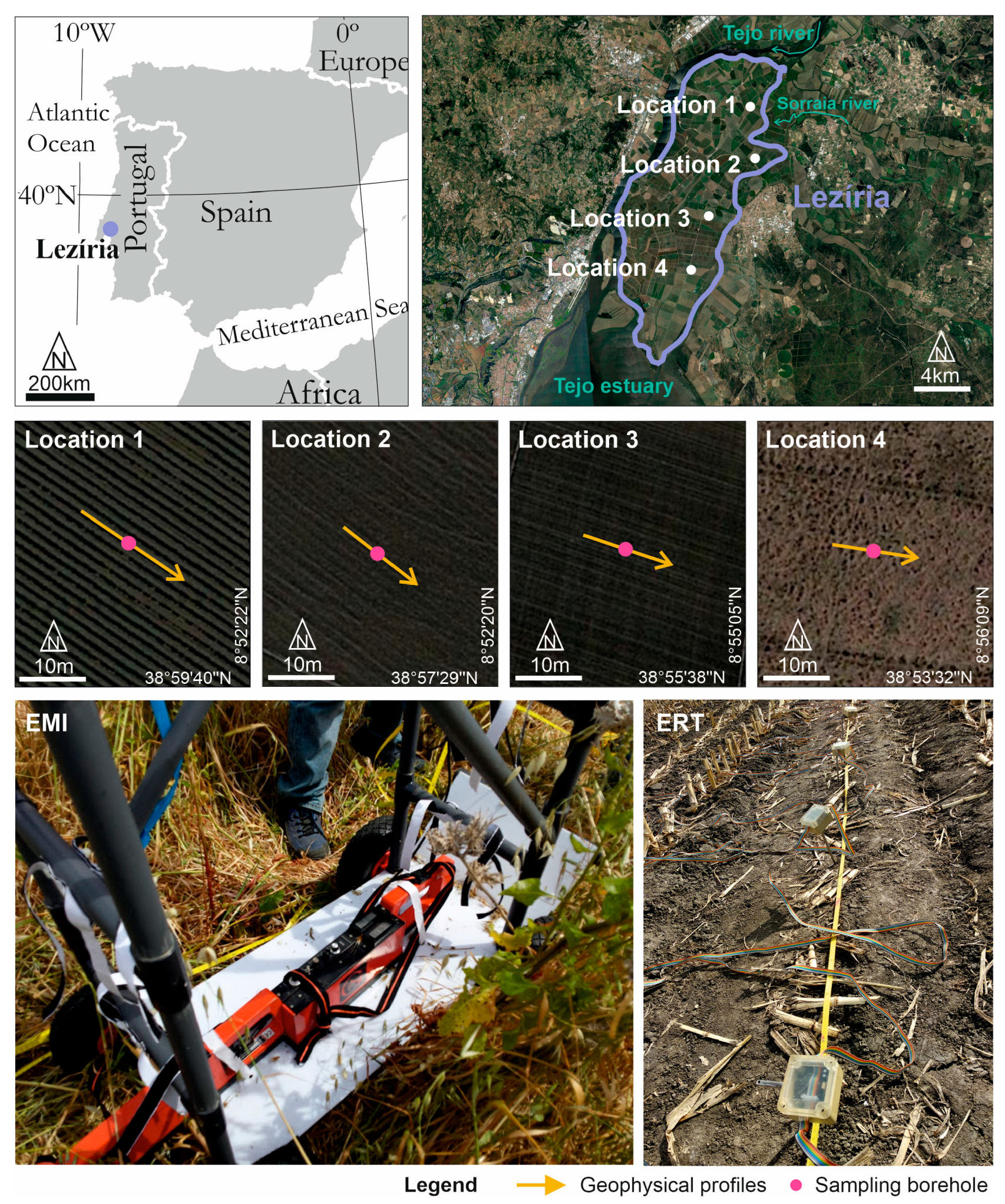
2.1. Study Area

The investigation was conducted in Lezíria de Vila Franca, situated 10 km northeast of Lisbon, Portugal (see Figure 1). It is a 130-square-kilometer alluvial peninsula bounded by the Tejo and Sorraia rivers. The climate is classified as temperate with hot and dry summers, according to the Köppen classification. In the northern region, the soils exhibit a fine to very fine texture and are categorized as Fluvisols, and in the southern region they are categorized as Solonchaks, based on the Harmonized World Soil Database [47]. There is a gradient of soil salinity that increases from north to south that affects the land use distribution. This gradient is a combination of (1) primary salinization [48], attributed to the regional presence of marine sediments and the saline influence of the estuary on groundwater in the southern part of the study area; and (2) secondary salinization [48], attributed to the irrigated farming that, using good quality water, has washed the soil in the northern part of the region. In fact, in this region, land use primarily comprises mainly irrigated annual crops in the north and rainfed pastures in the south.
For the comparative assessment, four distinct locations with varying salinity levels were selected within the study area (see Figure 1). According to the soil salinity classification defined by [49], location 1 exhibited non-saline conditions (ECe < 2 dS m−1), location 2 was slightly saline (2–4 dS m−1), location 3 was moderately to highly saline (4–16 dS m−1), and location 4 was severely saline, surpassing 16 dS m−1 at the time of the experiment [4,7,38].
Moreover, previous studies conducted by our team at this study area [4,7,38] have provided a detailed description of the soil’s physico-chemical properties. We have determined the pH, cation exchange capacity, and exchangeable sodium percentage. From this analysis, we know that all locations have a pH above 8 at depths below 30 cm, and that the exchangeable sodium percentage is above 15% in the subsoil at locations 2, 3, and 4. The latter indicates a high concentration of sodium in the soil exchange complex in relation to those of calcium and potassium. The principal component analysis showed that the soil electrical conductivity in this study area is mainly influenced by soil salinity [7]. This correlation is attributed to the significant north–south gradient of soil salinity, which predominates in influencing soil salinity impact, coupled with the limited variability observed in other soil properties like soil texture.
During the surveys, location 1 featured drip-irrigated tomatoes, and locations 2 and 3 centred on pivot irrigated maize, with no irrigation occurring on survey days. Location 4 is a rainfed natural pasture that had not been ploughed for at least the past decade.

2.2. Electromagnetic Induction

Electromagnetic induction (EMI, Figure 1) data were gathered, employing the EM38 instrument. The instrument comprises two coils housed in a case—one for transmiting the electromagnetic signal and the other for receiving it—positioned 1 m apart. The instrument can be oriented vertically (horizontal dipole mode) for a maximum depth of investigation of 1.5 m or horizontally (vertical dipole mode) for a maximum depth of 0.75 m. EMI surveys were conducted in the dry seasons of 2017 (locations 1 and 4) and 2018 (locations 2 and 3). ECa measurements were collected at 1 m intervals along a 20 m transect at each location (refer to Figure 1) and at two heights from the soil surface (0.15 and 0.4 m) in both horizontal and vertical dipole orientations. This positioning was facilitated by placing the EM38 on a custom-built cart for precision [38].
The inversion of ECa data to derive σ was executed using EM4SOIL software (V-3.05) [29]. The ECa responses in the model were determined through forward modelling based on the complete solution of the Maxwell equations [50]. The subsurface model employed in the inversion consisted of a series of 1-D models distributed according to the ECa measurement positions. Each subsurface model at a measurement position was influenced by neighbouring models, enabling algorithm use in regions characterized by high conductivity contrast. The inversion of ECa data employed an approach grounded in Occam regularization [51]. Data from all four locations were inverted, applying a five-layer earth initial model with an electrical conductivity of 100 mS m−1 and a fixed layer thickness of 0.30 m. The algorithm’s parameters, including the inversion algorithm type, number of iterations, and smoothing factor (λ) controlling model roughness, were chosen according to the methodology outlined in [38]. With the evenly distributed inverted data across the modelled area, 2D vertical σ models were generated for each location utilizing triangulation with linear interpolation.

2.3. Electrical Resistivity Tomography

Electrical resistivity tomography (ERT, Figure 1) data were acquired using a 4-point light 10 W system (LIPPMANN, Schaufling, Germany). The technology of this system is based on the measurement of voltage between two reading electrodes installed on the soil surface, when direct current is injected into two other electrodes, to calculate subsurface electrical resistivity. In this system, the disposition of the electrodes changes according to the array used, so that a grid of subsoil ERa values is obtained. The maximum depth of investigation and resolution vary with electrode spacing and the array configuration. ERT surveys were carried out at the same transects as EMI surveys, on the same dates, with electrode spacings of 1 m at location 1 and 0.75 m at locations 2, 3, and 4. ERa data were collected using the Wenner array, known for effective mapping in areas with significant vertical gradients of σ and a superior signal-to-noise ratio [31].
The inversion of ERa data to derive σ was performed using RES2DINV software (V-3.71) (Geotomo Software, Penang, Malaysia). Given the pronounced vertical salinity gradients due to saline groundwater in the region, robust inversion and mesh refinement to half of the electrode spacing were implemented to address anticipated strong resistivity contrasts. In robust inversion, the objective function aimed to minimize the absolute change in resistivity values, yielding models with well-defined interfaces between regions with varying resistivity values [31]. Since the inverted data were evenly distributed over the modelled area, 2D vertical σ models were produced for each location using triangulation with linear interpolation.

2.4. Soil Salinity

Soil samples were collected simultaneously as the geophysical surveys, in the medium point of each profile, as shown in Figure 1. There, five soil samples were collected between a depth of 0.15 m and 1.35 m representing topsoil (0–0.3 m), subsurface (0.3–0.6 m), upper subsoil (0.6–0.9 m), intermediate subsoil (0.9–1.2 m), and lower subsoil (1.2–1.5 m). It is noteworthy that the number of soil samples was limited to one borehole in each plot. This was because of the short length of the transects and the relatively small lateral variability of σ, suggesting that a single borehole could adequately represent soil properties. Furthermore, during the 18-month monitoring period at these four locations, a larger number of boreholes were drilled, and laboratory analysis confirmed the limited lateral variability of soil properties [4,7,38]. In the laboratory, ECe was determined using a conductivity meter (WTW 1C20-0211 inoLab) on liquid extracts obtained by suction filtering of the soil saturation paste derived from 300 g of air-dried and 2 mm sieved soil samples. The methodology employed for ECe measurement followed the procedures by [52], and soil samples’ salinity was classified according to [49], as described in Section 2.1.
Two regional calibrations were developed to predict ECe from all locations together, one using σ obtained from the inversion of EMI data and the other using σ obtained from the inversion of ERT data. The prediction ability of these calibrations was analysed through cross-validation, using the leave-one-out cross-validation in R language [53] through the function train(). In this method, one sample is removed and a calibration is established based on the remaining samples to predict the ECe of the removed sample. This procedure is iteratively repeated for each sample, until all 19 samples have been removed. The prediction ability of the calibrations was evaluated by calculating the root mean square errors (RMSE), and the mean errors (ME). RMSE evaluates matching between measured and predicted data, indicating more precise predictions when closer to zero. ME evaluates whether the predicted data are overestimated (negative ME) or underestimated (positive ME). RMSE and ME were calculated according to the following equations:
RMSE = i = 1 n ( mEC e i pEC e i ) 2 n
ME = i = 1 n ( mEC e i pEC e i ) n
where mECe indicates measured ECe and pECe indicates predicted ECe.
The two regional calibrations were then used to estimate ECe from σ (obtained from either EMI or ERT). Since the estimated ECe data were evenly distributed over the mapping area, 2D vertical soil salinity classification maps were produced for each location using triangulation with linear interpolation.

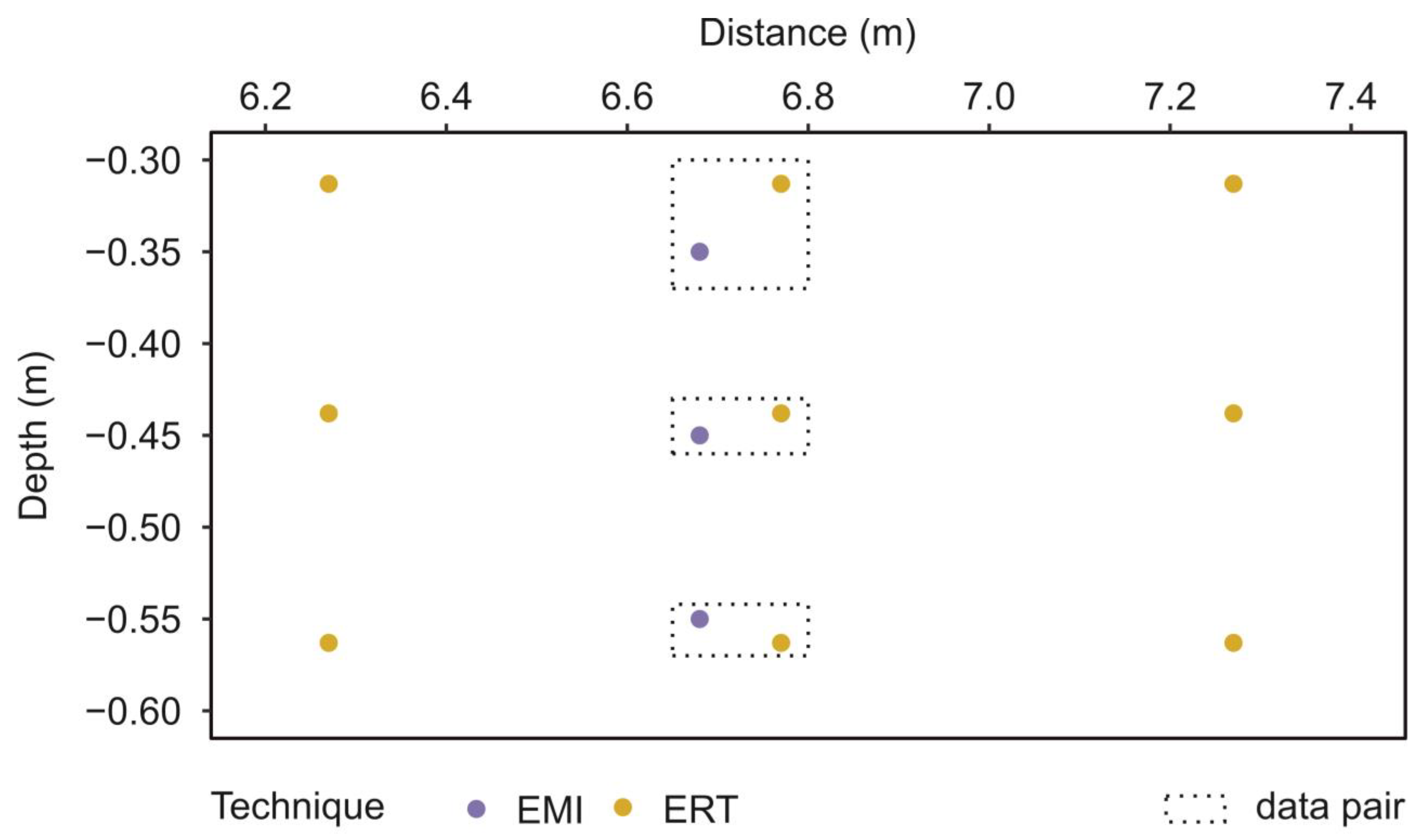
2.5. Agreement Analysis

Agreement analysis was performed for EMI and ERT techniques in estimating σ and ECe on the same points of the subsurface, based on the methodology described in [54]. In this methodology, the agreement is analysed using the differences between measurements made by two techniques on the same subject. In this study, we considered the subsurface position as the subject. However, both EMI and ERT data surveys and inversion processes produced subsurface σ grids that were not entirely coincident in space (Figure 2). To overcome this issue, σ grids obtained from EMI and ERT modelling results were ordered in data pairs selected for being distanced less than 0.22 m horizontally and 0.05 m vertically. This criterion was looser in the horizontal direction to maintain a statistically significant number of selected points, and it could be accepted because it was known from the previous studies [4,7,38] that the subsurface was highly horizontally stratified. The position attributed to each data pair was the position of the corresponding EMI measurement. These data pairs were then used for a comparison of EMI and ERT techniques in estimating σ, represented by (σERT, σEMI).
For the comparison of EMI and ERT techniques in predicting ECe, the data pairs used were composed by predicted ECe using ERT and predicted ECe using EMI, (pECe ERT, pECe EMI), and were located at the position of the soil samples, as a result of the procedure for the calibration development.
To visualize the agreement of σ, data pairs were represented through σEMI against σERT plots, and modified Bland–Altman plots [54]. In the latter type of plot, the difference between each data pair value is plotted against the mean between the two values, which represents the most approximate value to the true value being studied [54]. However, in this case, we used σERT in the y-axis, as we considered it to be the σ reference and true value. A reference interval within which fall most differences between the data is also included, and it is called the 95% limit of agreement [54]. The 95% limit of agreement can be calculated in different ways, depending on the differences between the data pair values following a normal distribution or not [54], which was investigated using the qqPlot function of R language [53].
When the normal distribution of the differences between the data pair values was verified, the 95% limits of agreement were calculated using the mean difference (MD) and the standard deviation (SD) of the differences as MD ± 1.96SD agreement [54]. MD and SD were calculated according to the following equations:
MD = i = 1 n ( σ EMI i σ ERT i ) n
SD = i = 1 n ( σ EMI i σ ERT i MD ) 2 n 1
When the normal distribution of the differences between the data pair values was not verified, the 95% limits of agreement were defined using the median (MeD), the 5 percentile (p5), and the 95 percentile (p95) of the differences [54].
To visualize the agreement between measured ECe and predicted ECe for each technique, data pairs were represented through another modification of the Bland–Altman plot, in which the difference between measured ECe and predicted ECe for each technique was plotted against the measured ECe.
Spearman’s rank correlation coefficient (RCC) between (i) the differences between σERT and σEMI, and σERT, for σ data, and (ii) the differences between measured ECe and predicted ECe, and the measured ECe, for ECe data, were calculated using the SpearmanRho() function of R language [53]. Spearman’s RCC always returns a value placed between −1 and 1. In this case, it would indicate if the differences between the values being compared are related to the magnitude of the property being estimated. A Spearman’s RCC closer to 1 means that the differences are closely related to the magnitude of the property being estimated [54].

3. Results and Discussion

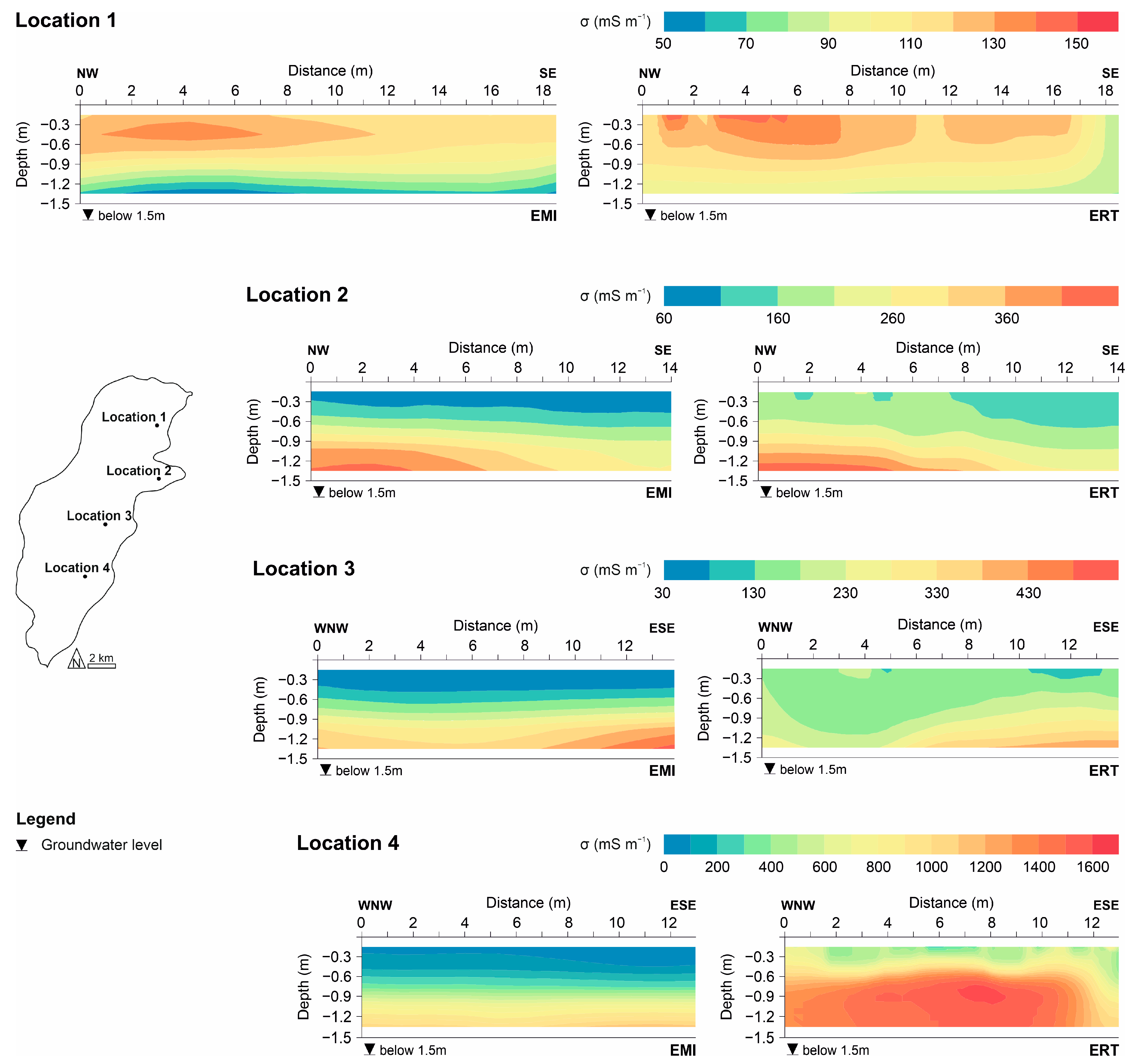
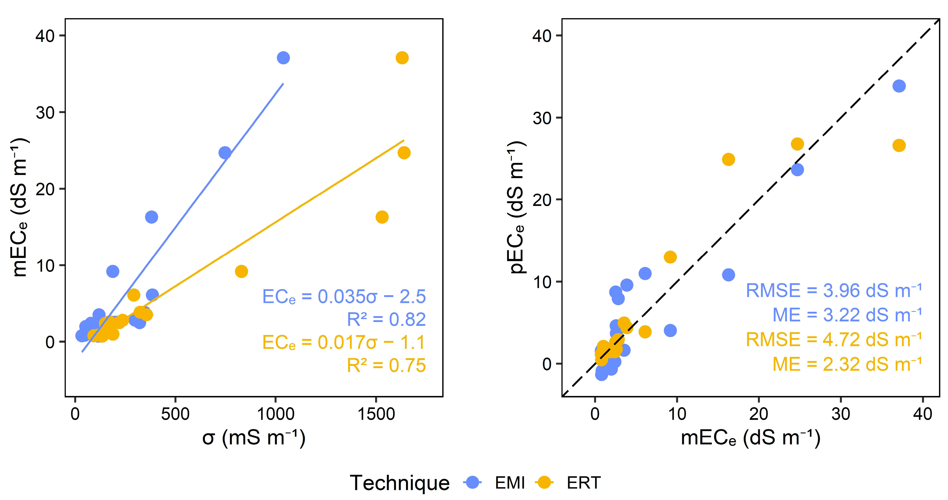
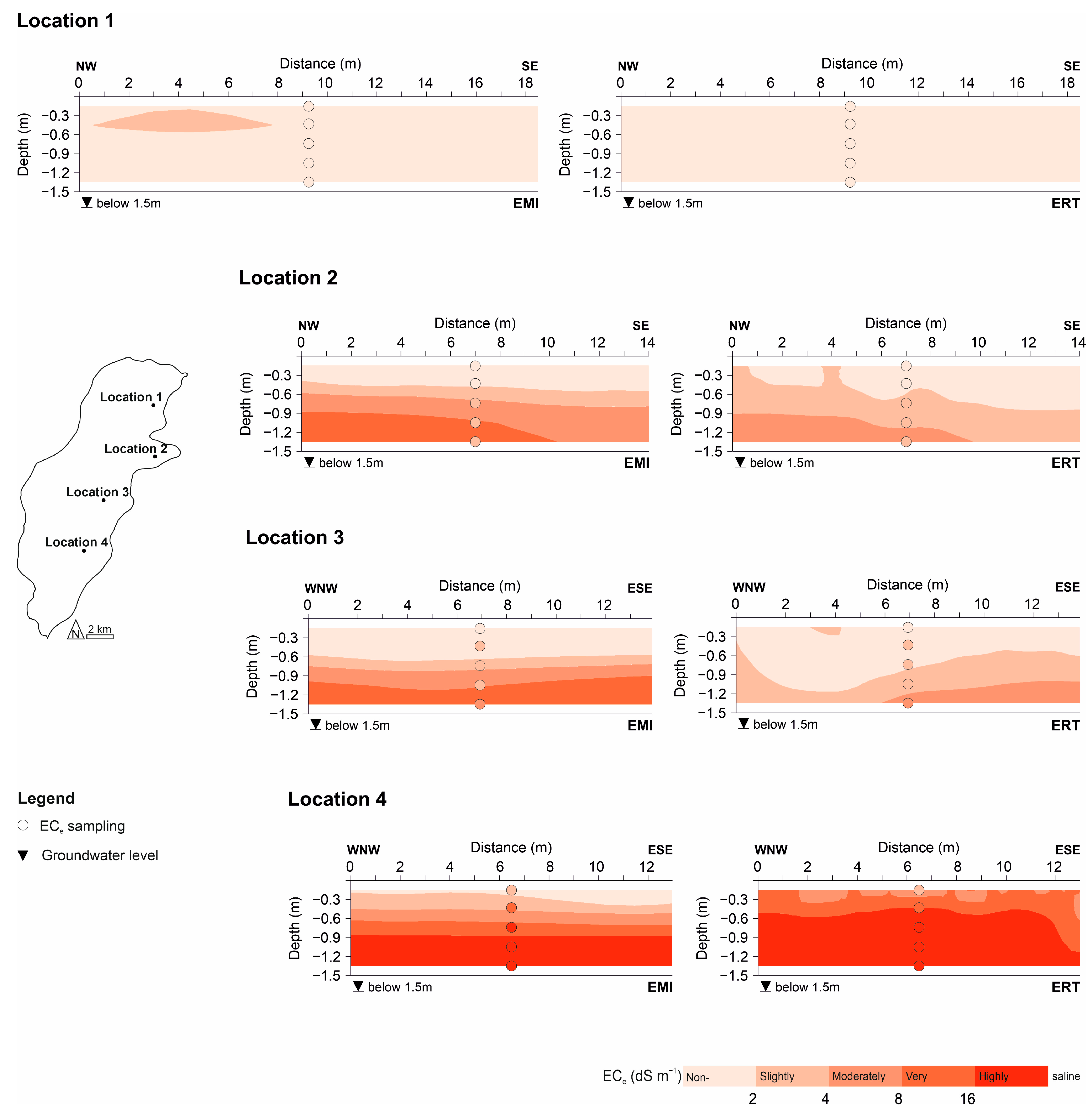
3.1. Soil Electrical Conductivity Obtained from EMI vs. ERT

Figure 3 shows the 2D vertical σ models obtained by EMI and by ERT techniques for locations 1 to 4. For both techniques, a general increasing trend of σ is evident from the north to the south of the peninsula, accompanying the known soil salinity gradient, illustrating the strong correlation of σ with ECe in the region, as verified previously in [4,7,38]. Also, both techniques show that σ increases with depth at locations 2, 3, and 4, which correlates well with groundwater depth and salinity in these locations. However, this trend is not observed at location 1, possibly due to irrigation and the deeper positioning of the saline groundwater at this site, making it less prone to capillary rise. Location 1 exhibits the lowest σ values, ranging from 50 to 160 mS m−1, followed by slightly higher σ values at location 2 (i.e., 60–460 mS m−1). Location 3 displays a greater variability in σ compared to the other two locations, featuring a minimum σ of 30 mS m−1 and a higher maximum of 530 mS m−1. The σ gradient at location 4, however, is the most substantial, with an extreme maximum σ of over 1600 mS m−1.
To compare the EMI model with ERT, Figure 4 shows the plots that support the agreement analysis between EMI and ERT σ estimations. At location 1, a normal distribution of the differences between σERT and σEMI data was verified, so the 95% limits of agreement were calculated using the mean difference (MD) and the standard deviation of the differences (SD), as explained in the Materials and Methods section. It could be verified that most differences between σERT data and σEMI data fell in the −14.98 mS m−1 to 32.16 mS m−1 interval. The mean difference was 8.59 mS m−1, and, since it was a positive value, indicated that, at this location, the EMI model tended to underestimate σ compared to the ERT model. This mean difference value was relatively low compared to the range of σERT data (82.20–143.10 mS m−1, Table 1). In terms of depths, agreement was generally good in topsoil (0–0.3 m), subsurface (0.3–0.6 m), and upper subsoil (0.6–0.9 m). However, the agreement diminished in the intermediate subsoil (0.9–1.2 m) and lower subsoil (1.2–1.5 m), as evidenced by the distance of points to the 1:1 line in the σEMI against σERT plot. Differences between σEMI and σERT data in the topsoil, subsurface, and upper subsoil were the closest to the 0-horizontal line in the Bland–Altman plot. The Bland–Altman plot indicates that, at this location, agreement increased with σ and decreased with depth. In comparison to the ERT model, there was an obvious tendency for the EMI model to underestimate σ in the lower subsoil (1.2–1.5 m). Spearman’s RCC of −0.34, as observed in location 1, indicates that generally the differences between σEMI and σERT are not related to the magnitude of σ.
At locations 2 to 4, a normal distribution of the differences between σEMI and σERT data was not verified, so the 95% limits of agreement were calculated using the median (MeD), the 5 percentile (p5), and the 95 percentile (p95) of the differences (see Section 2.5).
At location 2, most differences between σERT and σEMI data fell in the −24.88 mS m−1 to 77.19 mS m−1 interval. The median was 9.72 mS m−1, which indicates that, in general, at this location the EMI model similarly tended to underestimate σ, compared to the ERT model. Also, this value was low compared to the range of σERT data (126.70–446.20 mS m−1, Table 1). In terms of depth, agreement was generally good in the upper subsoil (0.6–0.9 m) and lower subsoil (1.2–1.5 m), which could be verified by the distance of points to the 1:1 line in the σEMI against σERT plot. Also, differences between σEMI data and σERT data in the upper and lower subsoil were the closest to the 0-horizontal line in the Bland–Altman plot. At this location, agreement increased with σ and with depth. This contrasted with the observations at location 1, where the most significant disagreement was noted in the lower subsoil (1.2–1.5 m). However, the distribution of σ at location 1 differed significantly from the variability observed in the other three locations, as σ decreased with depth at location 1. Spearman’s RCC of −0.54 indicates that generally, the differences between σEMI and σERT tend to slightly decrease when σ increases.
At location 3, most of the differences between σERT and σEMI data fell in the −126.62 mS m−1 to 107.34 mS m−1 interval. The median was 16.90 mS m−1, which indicates that, similar to locations 1 and 2, and in general, at this location the EMI model tended to underestimate σ, compared to the ERT model. Also, this value was low compared to the range of σERT data (107.40–427.50 mS m−1, Table 1). In terms of depth, agreement was generally good in the subsurface (0.3–0.6 m) and upper subsoil (0.6–0.9 m), as evidenced by the proximity of points to the 1:1 line in the σEMI against σERT plot and to the 0-horizontal line in the Bland–Altman plot. Spearman’s RCC of −0.65 indicates that the differences between σEMI and σERT slightly decrease when σ increases.
At location 4, most differences between σERT and σEMI data fell in the 291.90 mS m−1 to 1179.60 mS m−1 interval. This interval was totally above the 0-horizontal line in the Bland–Altman plot, which, together with a median of 667.72 mS m−1, indicated that at this location, the EMI model tended to drastically underestimate σ, compared to the ERT model. Also, this value was significantly high in the range of σERT data (356.40–1640.00 mS m−1, Table 1). In terms of depth, there was no significant agreement between σERT and σEMI, as evidenced by the lack of proximity of points to the 1:1 line in the σEMI against the σERT plot and to the 0-horizontal line in the Bland–Altman plot. Spearman’s RCC of 0.57 indicates that the differences between σEMI and σERT slightly increase when σ increases.
Comparing the results between locations suggests that the EMI models tend to underestimate σ when compared to the ERT models in all four locations. However, in locations 1, 2, and 3, with σ variability inferred from the ERT model in the 50–500 mS m−1 range, the underestimation of the EMI model was not significant, suggesting that the obtained EMI models were in good and acceptable agreement with those inferred from detailed ERT investigation. This was not the case at location 4, as the underestimation tendency was quite drastic at this location, where the σ variability inferred from the ERT model fell in the range of 500–1600 mS m−1. This is likely linked to the relationship between the quadrature component of the EMI signal and σ in superconductive soil at location 4, which may exhibit a non-monotonic behaviour [33]. In such situations, obtaining more representative ECa values may need the use of both the in-phase and quadrature components of the EMI signal [55]. However, the in-phase component has to be adequately calibrated, as it is susceptible to signal instability and offsets [56], which was not considered in this study. This presents a significant challenge when estimating σ in highly saline soil, where conductivity is anticipated to be extremely high. In this context, the robust ECa estimation approach, proposed by [57], may enhance the reliability of ECa estimation over superconductive areas. Alternatively, ERT (e.g., [44]) or TDR (e.g., [45]) measurements carried out along the same transects can be used to calibrate ECa data to obtain more representative ECa values.

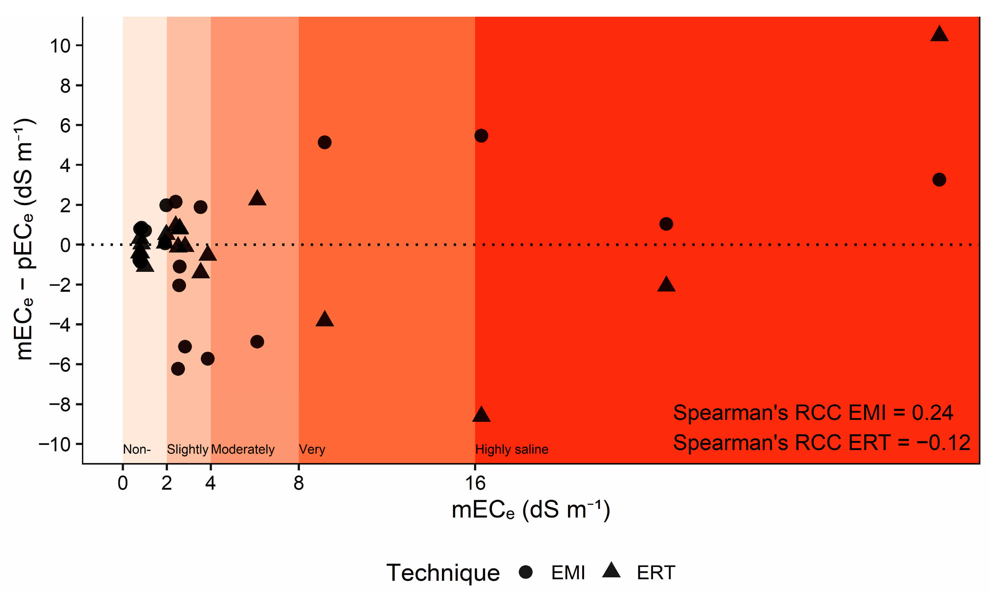
3.2. Soil Salinity Obtained from EMI vs. ERT

Figure 5 shows the two regional calibrations that were developed to predict ECe, one using the σ obtained from the inversion of EMI data and the other using σ, obtained from the inversion of ERT, and their prediction results. Both models had a strong R2, with EMI (0.86) being higher than ERT (0.75). The leave-one-out cross-validation resulted in acceptable and comparable RMSE and ME results. The obtained RMSE of 3.96 dS m–1 for EMI, and of 4.72 dS m–1 for ERT, were low in the measured ECe range (0.75–37.1 dS m–1, Table 1) and comparable between them. ME of 3.22 dS m–1 for EMI, and 2.32 dS m–1 for ERT, mean a comparable underestimation of the predicted data for both techniques.
Figure 6 shows the plot of the differences between measured ECe and predicted ECe, for each technique, against the measured ECe. The proximity of the points to the 0-horizontal line indicates that there is good agreement between measured and predicted ECe. Points above the line indicate underestimation, while points below the line indicate overestimation. In the non-saline classification interval of soil salinity, both techniques showed good agreement between measured and predicted ECe. In the slightly saline classification interval, EMI provided mostly overestimated predictions but also some underestimated predictions, whereas ERT showed good agreement between measured and predicted ECe. In the moderately saline classification interval, EMI provided one overestimated prediction, while ERT underestimated that same ECe measurement. In the very saline classification interval, EMI provided one underestimated prediction, while ERT overestimated that same ECe measurement. In the highly saline classification interval, the same happened as in the previous interval, except for one ECe measurement, which was underestimated by both techniques, but still classified as highly saline, for both techniques. Spearman’s RCC calculated for EMI (0.24) indicated that there was an underestimation tendency as the magnitude of ECe (soil salinity) increased. In the case of ERT, Spearman’s RCC of −0.12 indicated a slight overestimation tendency as the soil salinity grew.
A thorough examination of the calibrations reveals that, despite the EMI model significantly underestimating σ in the superconductive zone at location 4, resulting in a distinct linear regression slope between ECe and σ (EMI vs. ERT), this issue did not adversely affect the overall predictive capability of the regional calibration when compared to the results obtained from ERT. This is attributed to the fact that, although EMI underestimated σ at location 4, the pattern of σ distribution and its variations with depth aligned with those obtained from the ERT model.
To provide a better insight into the prediction ability of both methodologies in different locations, Figure 7 depicts the 2D vertical maps of soil salinity classification obtained from the conversion of σ obtained by EMI and ERT for locations 1 to 4, using the corresponding calibration. The filled-in circles in the maps represent the position and classification of the soil samples (measured ECe).
At location 1 there is total agreement between the predicted classification and the actual classification obtained from the samples, for both techniques. At location 2 soil salinity is overestimated by EMI at intermediate (0.9–1.2 m) and lower subsoil (1.2–1.5 m), while it is also overestimated by ERT but only in lower subsoil (1.2–1.5 m). At location 3, soil salinity is underestimated by EMI at the subsurface (0.3–0.9 m) and overestimated at intermediate (0.9–1.2 m) and lower subsoil (1.2–1.5 m), while it is underestimated by ERT at the subsurface (0.3–0.9 m) and upper subsoil (0.6–0.9 m). At location 4, soil salinity is underestimated by EMI from topsoil to upper subsoil (0–0.9 m), while there is total agreement between the predicted classification and the actual classification by ERT.
As anticipated, the salinity maps obtained from EMI and ERT are acceptably comparable, although EMI generally underestimated σ. Both techniques displayed similar levels of underestimations and overestimations, indicating a comparable level of prediction accuracy. The underestimation or overestimation of soil salinity based on σ is not only related to the geophysical approach but also influenced by the variability of other soil properties along the transects, such as soil texture, moisture content, salinity type, and temperature. For instance, in our previous study in the same study area, we observed that at location 2 the presence of slightly higher clay content in the subsoil, combined with the lower range of soil salinity (compared to locations 3 and 4), made it challenging to estimate ECe from EMI data and regional calibration [38]. Also, in the same study area, a relatively larger variability of moisture content and soil temperature in the topsoil at all locations was a major factor limiting ECe prediction in the topsoil [4]. Addressing such variability in soil properties may require location-specific calibration to consider soil texture and moisture variations, as discussed in [38]. Additionally, developing multiple regression models can account for the influence of other parameters on σ and soil salinity prediction. Nevertheless, since all measurements were conducted simultaneously at each location, we expect that comparable effects of other soil properties on both ERT and EMI techniques will not significantly impact the comparison between these two methodologies in assessing soil salinity, as they should have a similar effect on both.

4. Conclusions

In this study, EMI and ERT surveys and soil sampling were carried out at four locations with different salinity levels across the study area of Lezíria de Vila Franca, in dry season conditions, to analyse the agreement between the two techniques in estimating soil electrical conductivity and compare their ability in predicting soil salinity. While ERT may not offer a precise subsurface conductivity distribution of the subsoil (as no indirect method can achieve that), it stands out as one of the most reliable techniques for imaging the subsurface conductivity distribution. Conversely, EMI measurements are highly sensitive to various factors, including ground coupling, thermal drifts, and EM noise. Hence, it is sensible to consider an ERT inversion as a reference model that the EMI inversion should strive to approximate.
Based on the obtained results in this study, there was a reasonable agreement between the EMI and ERT models in three locations, where σ ranged from 50 to 500 mS m−1. In contrast, at location 4, where σ surpassed 1000 mS m−1, EMI notably underestimated σ in comparison to ERT. However, EMI models could still predict the increasing trend of σ well with depth. This suggests that the obtained EMI model may substantially underestimate σ in an extremely saline area given the very high level of soil conductivity, which exhibits a non-monotonic relationship between the quadrature component of the EMI signal. Under this condition, the σ values inferred from EMI modelling cannot be used alone to assess the soil salinity level without a location-specific regression or by applying a more robust approach to obtain a more representative ECa value. Further case studies across different soil types and salinity levels will offer more insights into the circumstances under which EMI performs optimally.
The regional calibrations based on both EMI and ERT demonstrated similar predictive capabilities. Despite the EMI model significantly underestimating σ in the superconductive zone at location 4, leading to a distinct regression linear slope between ECe and σ, this issue did not markedly affect the overall predictive performance of the regional calibration when compared to the results from ERT. This is because despite the underestimation of σ by EMI at location 4, the distribution pattern and depth-related variations in σ similarly mirrored those obtained from the ERT model, resulting in comparable prediction abilities.
Our case study was limited to four plots with distinct soil salinity levels, but with the same soil type. In addition, the number of soil samples was relatively limited, with one borehole for each location. Additional case studies across areas with different soil types and high conductivities are necessary to further evaluate the precision of EMI in soil salinity assessments. Specifically, EMI vs. ERT studies across sites with inverted soil salinity gradient in depth, where there is a superconductive zone over a more resistive zone, are particularly needed to assess the prediction ability of EMI in contrasting conditions, compared to this study. Larger numbers of boreholes and soil samples can also enhance the soil salinity prediction ability and the evaluation of the EMI prediction ability.
Lastly, we advise caution to EMI practitioners when working with superconductive soils. While it is not feasible to establish a definitive limit based solely on a single experiment using specific EMI equipment and across a study area with a similar soil type, our experiment indicated a significant underestimation σ in ranges above approximately 500 mS m−1. It is important to note that this finding may vary in different experiments across diverse soil and salinity types, as well as when using different EMI sensors. However, this does not diminish the concern regarding the challenge of using EMI in superconductive soil.

Author Contributions

Conceptualization, M.C.P. and M.F.; Data curation, N.L.C., M.F. and M.C.P.; Formal analysis, M.C.P. and M.F.; Funding acquisition, A.M.P., M.C.G. and F.M.S.; Investigation, M.C.P., N.L.C., A.M.P., M.C.G. and M.F.; Methodology, M.C.P., A.M.P., F.M.S. and M.F.; Project administration, M.C.G., F.M.S. and M.F.; Resources, N.L.C., A.M.P. and M.C.G.; Software, F.M.S.; Validation, M.C.P. and M.F.; Visualization, M.C.P.; Writing—original draft, M.C.P. and M.F.; Writing—review and editing, M.C.P., N.L.C., A.M.P., M.C.G., F.M.S. and M.F. All authors have read and agreed to the published version of the manuscript.

Funding

This work was funded by the Portuguese research agency, Fundação para a Ciência e a Tecnologia (FCT), in the scope of project SALTFREE—ARIMNET2/0004/2015 SALTFREE and ARIMNET2/0005/2015 SALTFREE. This work was also supported by the European Joint Programme Cofund on Agricultural Soil Management (EJP SOIL grant number 862695), funded by the European Union’s Horizon H2020 research and innovation project, and was carried out in the framework of the STEROPES of EJP-SOIL.

Data Availability Statement

The data presented in this study are available on request from the corresponding author. The data are not publicly available due to having been acquired at privately owned farms.

Acknowledgments

The authors express their appreciation to the Associação de Beneficiários da Lezíria Grande de Vila Franca de Xira for granting access to study sites and for their ongoing support. Special thanks are also extended to Manuel Fernandes and Fernando Pires from INIAV for their field assistance. This work was funded by the Portuguese Fundação para a Ciência e a Tecnologia (FCT) I.P./MCTES through national funds (PIDDAC)—UIDB/50019/2020 (https://doi.org/10.54499/UIDB/50019/2020 accessed on 21 February 2024), UIDP/50019/2020 (https://doi.org/10.54499/UIDP/50019/2020 accessed on 21 February 2024) and LA/P/0068/2020 (https://doi.org/10.54499/LA/P/0068/2020 accessed on 21 February 2024).

Conflicts of Interest

The authors declare no conflict of interests.

References

  1. Corwin, D.L.; Scudiero, E. Chapter One—Review of Soil Salinity Assessment for Agriculture across Multiple Scales Using Proximal and/or Remote Sensors. In Advances in Agronomy; Sparks, D.L., Ed.; Academic Press: Cambridge, MA, USA, 2019; Volume 158, pp. 1–130. [Google Scholar]
  2. Corwin, D.L.; Lesch, S.M. Apparent Soil Electrical Conductivity Measurements in Agriculture. Comput. Electron. Agric. 2005, 46, 11–43. [Google Scholar] [CrossRef]
  3. Rhoades, J.D.; Corwin, D.L.; Lesch, S.M. Geospatial Measurements of Soil Electrical Conductivity to Assess Soil Salinity and Diffuse Salt Loading from Irrigation. In Assessment of Non-Point Source Pollution in the Vadose Zone; American Geophysical Union (AGU): Washington, DC, USA, 1999; pp. 197–215. ISBN 9781118664698. [Google Scholar]
  4. Paz, M.C.; Farzamian, M.; Paz, A.M.; Castanheira, N.L.; Gonçalves, M.C.; Santos, F.M. Assessing Soil Salinity Dynamics Using Time-Lapse Electromagnetic Conductivity Imaging. SOIL 2020, 6, 499–511. [Google Scholar] [CrossRef]
  5. Nguyen, V.H.; Germer, J.; Duong, V.N.; Asch, F. Soil Resistivity Measurements to Evaluate Subsoil Salinity in Rice Production Systems in the Vietnam Mekong Delta. Near Surf. Geophys. 2023, 21, 288–299. [Google Scholar] [CrossRef]
  6. Innocenti, A.; Pazzi, V.; Napoli, M.; Fanti, R.; Orlandini, S. Application of Electrical Resistivity Tomography (ERT) to Study to Soil Water and Salt Movement under Drip Irrigation in a Saline Soil Cultivated with Melon. In Proceedings of the EGU General Assembly Conference Abstracts, Vienna, Austria, 3–8 April 2022; pp. EGU22–4469. [Google Scholar]
  7. Paz, A.M.; Castanheira, N.; Farzamian, M.; Paz, M.C.; Gonçalves, M.C.; Monteiro Santos, F.A.; Triantafilis, J. Prediction of Soil Salinity and Sodicity Using Electromagnetic Conductivity Imaging. Geoderma 2020, 361, 114086. [Google Scholar] [CrossRef]
  8. da Silva, L.D.C.M.; Peixoto, D.S.; Azevedo, R.P.; Avanzi, J.C.; Junior, M.D.S.D.; Vanella, D.; Consoli, S.; Acuña-Guzman, S.F.; Borghi, E.; de Resende, Á.V.; et al. Assessment of Soil Water Content Variability Using Electrical Resistivity Imaging in an Oxisol under Conservation Cropping Systems. Geoderma Reg. 2023, 33, e00624. [Google Scholar] [CrossRef]
  9. Beff, L.; G ¨ Unther, T.; Vandoorne, B.; Couvreur, V.; Javaux, M. Three-Dimensional Monitoring of Soil Water Content in a Maize Field Using Electrical Resistivity Tomography. Hydrol. Earth Syst. Sci 2013, 17, 595–609. [Google Scholar] [CrossRef]
  10. Guan, Y.; Grote, K.; Schott, J.; Leverett, K. Prediction of Soil Water Content and Electrical Conductivity Using Random Forest Methods with UAV Multispectral and Ground-Coupled Geophysical Data. Remote Sens. 2022, 14, 1023. [Google Scholar] [CrossRef]
  11. Ratshiedana, P.E.; Abd Elbasit, M.A.M.; Adam, E.; Chirima, J.G.; Liu, G.; Economon, E.B. Determination of Soil Electrical Conductivity and Moisture on Different Soil Layers Using Electromagnetic Techniques in Irrigated Arid Environments in South Africa. Water 2023, 15, 1911. [Google Scholar] [CrossRef]
  12. de Jong, S.M.; Heijenk, R.A.; Nijland, W.; van der Meijde, M. Monitoring Soil Moisture Dynamics Using Electrical Resistivity Tomography under Homogeneous Field Conditions. Sensors 2020, 20, 5313. [Google Scholar] [CrossRef]
  13. Acosta, J.A.; Gabarrón, M.; Martínez-Segura, M.; Martínez-Martínez, S.; Faz, Á.; Pérez-Pastor, A.; Gómez-López, M.D.; Zornoza, R. Soil Water Content Prediction Using Electrical Resistivity Tomography (ERT) in Mediterranean Tree Orchard Soils. Sensors 2022, 22, 1365. [Google Scholar] [CrossRef]
  14. Shanahan, P.W.; Binley, A.; Whalley, W.R.; Watts, C.W. The Use of Electromagnetic Induction to Monitor Changes in Soil Moisture Profiles beneath Different Wheat Genotypes. Soil Sci. Soc. Am. J. 2015, 79, 459–466. [Google Scholar] [CrossRef]
  15. Whalley, W.R.; Binley, A.; Watts, C.W.; Shanahan, P.; Dodd, I.C.; Ober, E.S.; Ashton, R.W.; Webster, C.P.; White, R.P.; Hawkesford, M.J. Methods to Estimate Changes in Soil Water for Phenotyping Root Activity in the Field. Plant Soil 2017, 415, 407–422. [Google Scholar] [CrossRef]
  16. Zhao, X.; Wang, J.; Zhao, D.; Li, N.; Zare, E.; Triantafilis, J. Digital Regolith Mapping of Clay across the Ashley Irrigation Area Using Electromagnetic Induction Data and Inversion Modelling. Geoderma 2019, 346, 18–29. [Google Scholar] [CrossRef]
  17. Triantafilis, J.; Lesch, S.M. Mapping Clay Content Variation Using Electromagnetic Induction Techniques. Comput. Electron. Agric. 2005, 46, 203–237. [Google Scholar] [CrossRef]
  18. Huang, J.; Lark, R.M.; Robinson, D.A.; Lebron, I.; Keith, A.M.; Rawlins, B.; Tye, A.; Kuras, O.; Raines, M.; Triantafilis, J. Scope to Predict Soil Properties at Within-Field Scale from Small Samples Using Proximally Sensed γ-Ray Spectrometer and EM Induction Data. Geoderma 2014, 232–234, 69–80. [Google Scholar] [CrossRef]
  19. Zare, E.; Li, N.; Khongnawang, T.; Farzamian, M.; Triantafilis, J. Identifying Potential Leakage Zones in an Irrigation Supply Channel by Mapping Soil Properties Using Electromagnetic Induction, Inversion Modelling and a Support Vector Machine. Soil Syst. 2020, 4, 25. [Google Scholar] [CrossRef]
  20. Triantafilis, J.; Lesch, S.M.; La Lau, K.; Buchanan, S.M. Field Level Digital Soil Mapping of Cation Exchange Capacity Using Electromagnetic Induction and a Hierarchical Spatial Regression Model. Soil Res. 2009, 47, 651–663. [Google Scholar] [CrossRef]
  21. Koganti, T.; Narjary, B.; Zare, E.; Pathan, A.L.; Huang, J.; Triantafilis, J. Quantitative Mapping of Soil Salinity Using the DUALEM-21S Instrument and EM Inversion Software. Land Degrad. Dev. 2018, 29, 1768–1781. [Google Scholar] [CrossRef]
  22. Zhao, D.; Li, N.; Zare, E.; Wang, J.; Triantafilis, J. Mapping Cation Exchange Capacity Using a Quasi-3d Joint Inversion of EM38 and EM31 Data. Soil Tillage Res. 2020, 200, 104618. [Google Scholar] [CrossRef]
  23. Zhao, X.; Wang, J.; Zhao, D.; Sefton, M.; Triantafilis, J. Mapping Cation Exchange Capacity (CEC) Across Sugarcane Fields with Different Comparisons by Using DUALEM Data. J. Environ. Eng. Geophys. 2023, 27, 191–205. [Google Scholar] [CrossRef]
  24. Huang, J.; Pedrera-Parrilla, A.; Vanderlinden, K.; Taguas, E.V.; Gómez, J.A.; Triantafilis, J. Potential to Map Depth-Specific Soil Organic Matter Content across an Olive Grove Using Quasi-2d and Quasi-3d Inversion of DUALEM-21 Data. CATENA 2017, 152, 207–217. [Google Scholar] [CrossRef]
  25. Jupp, D.L.B.; Vozoff, K. Stable Iterative Methods for the Inversion of Geophysical Data. Geophys. J. R. Astron. Soc. 1975, 42, 957–976. [Google Scholar] [CrossRef]
  26. Monteiro Santos, F.A. 1-D Laterally Constrained Inversion of EM34 Profiling Data. J. Appl. Geophys. 2004, 56, 123–134. [Google Scholar] [CrossRef]
  27. Moghadas, D. Probabilistic Inversion of Multiconfiguration Electromagnetic Induction Data Using Dimensionality Reduction Technique: A Numerical Study. Vadose Zone J. 2019, 18, 180183. [Google Scholar] [CrossRef]
  28. Narciso, J.; Bobe, C.; Azevedo, L.; Van De Vijver, E. A Comparison between Kalman Ensemble Generator and Geostatistical Frequency-Domain Electromagnetic Inversion: The Impacts on near-Surface Characterization. Geophysics 2022, 87, E335–E346. [Google Scholar] [CrossRef]
  29. EMTOMO. Manual for EM4Soil: A Program for 1-D Laterally Constrained Inversion of EM Data; EMTOMO: Lisbon, Portugal, 2018. [Google Scholar]
  30. McLachlan, P.; Blanchy, G.; Binley, A. EMagPy: Open-Source Standalone Software for Processing, Forward Modeling and Inversion of Electromagnetic Induction Data. Comput. Geosci. 2021, 146, 104561.EM. [Google Scholar] [CrossRef]
  31. Loke, M.H. Rapid 2D Resistivity Forward Modeling Using the Finite Difference and Finite Element Methods. RES2DMOD Ver 2002, 3, 1996–2002. [Google Scholar]
  32. Rücker, C.; Günther, T.; Wagner, F.M. PyGIMLi: An Open-Source Library for Modelling and Inversion in Geophysics. Comput. Geosci. 2017, 109, 106–123. [Google Scholar] [CrossRef]
  33. Blanchy, G.; Saneiyan, S.; Boyd, J.; McLachlan, P.; Binley, A. ResIPy, an Intuitive Open Source Software for Complex Geoelectrical Inversion/Modeling. Comput. Geosci. 2020, 137, 104423. [Google Scholar] [CrossRef]
  34. Araújo, O.S.; Picotti, S.; Francese, R.G.; Bocchia, F.; Santos, F.M.; Giorgi, M.; Tessarollo, A. Frequency Domain Electromagnetic Calibration for Improved Detection of Sand Intrusions in River Embankments. Lead. Edge 2023, 42, 615–624. [Google Scholar] [CrossRef]
  35. FAO. Global Map of Salt-Affected Soils. Available online: https://www.fao.org/soils-portal/data-hub/soil-maps-and-databases/global-map-of-salt-affected-soils/ar/ (accessed on 21 February 2024).
  36. Stavi, I.; Thevs, N.; Priori, S. Soil Salinity and Sodicity in Drylands: A Review of Causes, Effects, Monitoring, and Restoration Measures. Front. Environ. Sci. 2021, 9, 330. [Google Scholar] [CrossRef]
  37. Paz, A.M.; Amezketa, E.; Canfora, L.; Castanheira, N.; Falsone, G.; Gonçalves, M.C.; Gould, I.; Hristov, B.; Mastrorilli, M.; Ramos, T.; et al. Salt-Affected Soils: Field-Scale Strategies for Prevention, Mitigation, and Adaptation to Salt Accumulation. Ital. J. Agron. 2023, 18, 2166. [Google Scholar] [CrossRef]
  38. Farzamian, M.; Paz, M.C.; Paz, A.M.; Castanheira, N.L.; Gonçalves, M.C.; Monteiro Santos, F.A.; Triantafilis, J. Mapping Soil Salinity Using Electromagnetic Conductivity Imaging—A Comparison of Regional and Location-Specific Calibrations. L. Degrad. Dev. 2019, 30, 1393–1406. [Google Scholar] [CrossRef]
  39. Khongnawang, T.; Zare, E.; Srihabun, P.; Khunthong, I.; Triantafilis, J. Digital Soil Mapping of Soil Salinity Using EM38 and Quasi-3d Modelling Software (EM4Soil). Soil Use Manag. 2022, 38, 277–291. [Google Scholar] [CrossRef]
  40. Lavoué, F.; van der Krak, J.; Rings, J.; André, F.; Moghadas, D.; Huisman, J.A.; Lambot, S.; Weiherrnüller, L.; Vanderborght, J.; Vereecken, H. Electromagnetic Induction Calibration Using Apparent Electrical Conductivity Modelling Based on Electrical Resistivity Tomography. Near Surf. Geophys. 2010, 8, 553–561. [Google Scholar] [CrossRef]
  41. Minsley, B.J.; Smith, B.D.; Hammack, R.; Sams, J.I.; Veloski, G. Calibration and Filtering Strategies for Frequency Domain Electromagnetic Data. J. Appl. Geophys. 2012, 80, 56–66. [Google Scholar] [CrossRef]
  42. Moghadas, D.; Jadoon, K.Z.; McCabe, M.F. Spatiotemporal Monitoring of Soil Water Content Profiles in an Irrigated Field Using Probabilistic Inversion of Time-Lapse EMI Data. Adv. Water Resour. 2017, 110, 238–248. [Google Scholar] [CrossRef]
  43. von Hebel, C.; Rudolph, S.; Mester, A.; Huisman, J.A.; Kumbhar, P.; Vereecken, H.; van der Kruk, J. Three-Dimensional Imaging of Subsurface Structural Patterns Using Quantitative Large-Scale Multiconfiguration Electromagnetic Induction Data. Water Resour. Res. 2014, 50, 2732–2748. [Google Scholar] [CrossRef]
  44. Von Hebel, C.; Van Der Kruk, J.; Huisman, J.A.; Mester, A.; Altdorff, D.; Endres, A.L.; Zimmermann, E.; Garré, S.; Vereecken, H. Calibration, Conversion, and Quantitative Multi-Layer Inversion of Multi-Coil Rigid-Boom Electromagnetic Induction Data. Sensors 2019, 19, 4753. [Google Scholar] [CrossRef] [PubMed]
  45. Dragonetti, G.; Comegna, A.; Ajeel, A.; Deidda, G.P.; Lamaddalena, N.; Rodriguez, G.; Vignoli, G.; Coppola, A. Calibrating Electromagnetic Induction Conductivities with Time-Domain Reflectometry Measurements. Hydrol. Earth Syst. Sci. 2018, 22, 1509–1523. [Google Scholar] [CrossRef]
  46. Dragonetti, G.; Farzamian, M.; Basile, A.; Monteiro Santos, F.; Coppola, A. In Situ Estimation of Soil Hydraulic and Hydrodispersive Properties by Inversion of Electromagnetic Induction Measurements and Soil Hydrological Modeling. Hydrol. Earth Syst. Sci. 2022, 26, 5119–5136. [Google Scholar] [CrossRef]
  47. Fischer, G.; Nachtergaele, F.O.; Prieler, S.; Teixeira, E.; Toth, G.; van Velthuizen, H.; Verelst, L.; Wiberg, D. Global Agro-Ecological Zones (GAEZ v3.0)-Model Documentation 2012. Available online: https://www.gaez.iiasa.ac.at/docs/GAEZ_Model_Documentation.pdf (accessed on 21 February 2024).
  48. Daliakopoulos, I.N.; Tsanis, I.K.; Koutroulis, A.; Kourgialas, N.N.; Varouchakis, A.E.; Karatzas, G.P.; Ritsema, C.J. The Threat of Soil Salinity: A European Scale Review. Sci. Total Environ. 2016, 573, 727–739. [Google Scholar] [CrossRef]
  49. Barrett-Lennard, E.; Bennett, S.; Colmer, T. Standardising Terminology for Describing the Level of Salinity in Soils in Australia. In Proceedings of the 2nd International Salinity Forum. Salinity, Water and Society: Global Issues, Local Action, Adelaide, Australia, 30 March–3 April 2008; Future Farm Industries CRC: Perth, WA, Australia; University of Western Australia: Crawley, WA, Australia, 2008. [Google Scholar]
  50. Kaufman, A.; Keller, G.V. Frequency and Transient Sounding Methods in Geochemistry and Geophysics, Vol. 16 A, A. Kaufman and G. V. Keller, Elsevier, Amsterdam, 1983 686 pp. £85.55/$144.75. Geophys. J. Int. 1984, 77, 935–937. [Google Scholar] [CrossRef]
  51. deGroot-Hedlin, C.; Constable, S. Occam’s Inversion to Generate Smooth, Two-dimensional Models from Magnetotelluric Data. Geophysics 1990, 55, 1613–1624. [Google Scholar] [CrossRef]
  52. Allison, L.E.; Bernstein, L.; Bower, C.A.; Brown, J.W.; Fireman, M.; Hatcher, J.T.; Hayward, H.E.; Pearson, G.A.; Reeve, R.C.; Richards, L.A.; et al. Diagnosis and Improvement of Saline Alkali Soils, Agricultural Handbook; Richards, L.A., Ed.; United States Department of Agriculture: Washington, DC, USA, 1954.
  53. R Core Team. R: A Language and Environment for Statistical Computing; R Foundation for Statistical Computing: Vienna, Austria, 2020. [Google Scholar]
  54. Bland, J.M.; Altman, D.G. Measuring Agreement in Method Comparison Studies. Stat. Methods Med. Res. 1999, 8, 135–160. [Google Scholar] [CrossRef]
  55. Guillemoteau, J.; Sailhac, P.; Boulanger, C.; Trules, J. Inversion of Ground Constant Offset Loop-Loop Electromagnetic Data for a Large Range of Induction Numbers. Geophysics 2015, 80, E11–E21. [Google Scholar] [CrossRef]
  56. De Smedt, P.; Delefortrie, S.; Wyffels, F. Identifying and Removing Micro-Drift in Ground-Based Electromagnetic Induction Data. J. Appl. Geophys. 2016, 131, 14–22. [Google Scholar] [CrossRef]
  57. Hanssens, D.; Delefortrie, S.; Bobe, C.; Hermans, T.; De Smedt, P. Improving the Reliability of Soil EC-Mapping: Robust Apparent Electrical Conductivity (RECa) Estimation in Ground-Based Frequency Domain Electromagnetics. Geoderma 2019, 337, 1155–1163. [Google Scholar] [CrossRef]
Figure 1. Location of Lezíria, the study area, details of the four locations with the geophysical transects and soil sampling sites, and images of the electromagnetic induction (EMI) and electrical resistivity tomography (ERT) instruments used in geophysical acquisition. © Google Earth.
Land 13 00295 g001
Figure 2. Comparison of electromagnetic induction (EMI) and electrical resistivity tomography (ERT) σ grids for location 1, Lezíria, Portugal.
Land 13 00295 g002
Figure 3. Two-dimensional vertical soil electrical conductivity (σ) models obtained from electromagnetic induction (EMI, left) and electrical resistivity tomography (ERT, right) techniques for locations 1 to 4.
Land 13 00295 g003
Figure 4. Agreement of soil electrical conductivity (σ) obtained from electromagnetic induction (EMI) and electrical resistivity tomography (ERT) techniques for locations 1 to 4: σEMI against σERT plots with the 1:1 line (left), and modified Bland–Altman plots with the 95% limits of agreement (right). Plots include the number of data (n) (left), Spearman’s rank correlation coefficient (RCC), mean difference (MD), standard deviation (SD), median (MeD), the 5 percentile (p5), and the 95 percentile (p95) (right).
Land 13 00295 g004
Figure 5. Measured soil salinity (mECe) versus soil electrical conductivity (σ) obtained from electromagnetic induction (EMI) and electrical resistivity tomography (ERT) techniques for the regional calibrations (left), and predicted soil salinity (pECe) obtained from the leave-one-out-cross-validation of the calibrations (right). Plots include calibrations and their coefficient of determination (R2) (left), and their root mean square error (RMSE) and mean error (ME).
Land 13 00295 g005
Figure 6. Agreement of measured soil salinity (mECe) and predicted soil salinity (pECe) obtained using electromagnetic induction (EMI) and electrical resistivity tomography (ERT) techniques, with Spearman’s rank correlation coefficient (RCC).
Land 13 00295 g006
Figure 7. Two-dimensional vertical soil salinity classification maps obtained by electromagnetic induction (EMI, left) and electrical resistivity tomography (ERT, right) techniques for locations 1 to 4. The filled circles represent the position and classification of the soil samples (measured ECe).
Land 13 00295 g007
Table 1. Statistics of soil’s electrical conductivity obtained from electrical resistivity tomography (σERT), and measured soil salinity (mECe): minimum, maximum, range, and amount of data, at locations 1 to 4 and at all locations together, respectively.
UnitLocationMinimumMaximumRangeAmount of Data
σERTmS m−1182.20143.1060.9080
2126.70446.20319.50252
3107.40427.50320.10252
4356.401640.001283.60196
mECedS m−1all0.7537.1036.7519
σERT is soil electrical conductivity obtained by electrical resistivity tomography. mECe is measured soil salinity obtained from saturated soil paste extract (ECe).
Disclaimer/Publisher’s Note: The statements, opinions and data contained in all publications are solely those of the individual author(s) and contributor(s) and not of MDPI and/or the editor(s). MDPI and/or the editor(s) disclaim responsibility for any injury to people or property resulting from any ideas, methods, instructions or products referred to in the content.

