Comparing Two Saline-Gypseous Wetland Soils in NE Spain

Abstract

Small (<1 km²) saline wetlands scattered across the landscape often go unnoticed or are threatened by urbanization or other interventions, despite their role as biodiversity shelters. This study is needed to show methods for monitoring this specific kind of wetland, and to guide the selection of analytical techniques. We provide data and comparisons for salient soil traits of two quasi-pristine gypsiferous and saline wetlands named Farrachuela (FA) and Agustín (AG). The soil characteristics presented in this article are a more sensitive indicator of their ecological status than some of the most used indicators, such as birds and plants. We found significant differences between the two saladas in percent water saturation, equivalent calcium carbonate, gypsum content, and soil salinity expressed as electrical conductivity both of 1:5 soil-to-water ratio and of saturation extracts. The differences were also significant in the concentrations of Mg²⁺, Na⁺, and Cl⁻, while they were non-significant for Ca²⁺, HCO₃²⁻, and SO₄²⁻. The mean contents of the six ions were lower in FA than in AG. Both pH and sodium adsorption ratios were significantly different between the two wetlands. The data are mainly examined and plotted by displaying their non-parametric statistics, a synoptic approach that will allow us to monitor the evolution of the wetlands against both traditional agricultural pressures and emerging green energy infrastructures. Last but not least, we discuss the shortcomings of some standard laboratory methods when applied to gypsum-rich soils.

1. Introduction

European inland saline habitats have been quasi-eliminated [1], with many of the surviving ones reduced in size or badly degraded. This is also the case in the arid Central Ebro Basin, Spain [2]. The scarcity of regulations or incentives for protecting soil diversity occurs in several European countries [3] and is more pronounced for inland saline wetlands in general.

This scarcity also happens for the lands whose composition, color, vegetation or other characteristics are due to an abundance of gypsum (CaSO₄•2H₂O). These whitish gypsum soil landscapes, known by local people in NE Spain as chesas, occur mainly in warm countries around the world [4], but also in cold regions with gyprock outcrops, e.g., [5,6]. Chesas have also been traditionally disdained due to their low agricultural production and geotechnical characteristics. Irrigation of these lands, needed in dry areas for agricultural production, is technically unfeasible by inundation due to the solubility of gypsum, and only the pressurized application of water has alleviated the drawbacks. The disdain is counteracted by the agricultural pressure and by the increasing attention of scientists to the gypsophilous plants protected by environmental rules [7]. Thus, saline wetlands located in gypseous soils pose a double challenge to life, and are therefore of twofold interest to science. Moreover, the study and description of these saline wetlands face methodological issues in their lab analyses―often overlooked in the literature―derived from the abundance of gypsum [4,8].

The old judgment on both the wetlands and the gypseous soils based on their little or no agricultural value is evolving towards legal protection due to the biodiversity they harbor and their role in ecological balances. In addition, insights into biodiversity and ecosystem services raise the need to move beyond single-lake thinking [9] and to include the small wetlands [10], a line of reasoning that also applies to gypseous soils. Together with the coexistence with agriculture, including irrigation and intensive animal husbandry, there now arise threats from the “green energy” sources with several kinds of impacts, such as those recently reported in [11,12].

The Ebro Basin, located in northeastern Spain (Figure 1), has a dry climate and a high presence of gypsum rocks 1.9 10⁶ hectares of gypsiferous lithofacies [13] together with many landscape evidences of salinity, such as saline ravines associated with springs or oozing sources, and especially many endorheic saline wetlands and saline depressions. Some of these wetlands had artisanal salterns until one century ago. Nowadays, these athalassohaline wetlands —locally named saladas— are hot spots for nature conservation due to the rare or singular habitats they host. Scientific interest in these wetlands can be traced back to the 19th century. The data set [14] lists many works describing the physical conditions, geology, soils, vegetation, and other features of the saladas of Sástago-Bujaraloz in the Central Ebro Basin, an endorheic complex included in the RAMSAR list. Salada Agustín is included in this complex. By contrast, salada Farrachuela located in the chesas of the Barbastro Gypsum Formation, about 70 km NE of salada Agustín (Figure 1), is isolated and went unnoticed by scientists until recently. This kind of wetland is found in areas with arid or Mediterranean climates, but is also comparable to wetlands developed in gypsum karst depressions in cold climates [6].

Protection of the European saladas should be implemented throughout the Natura 2000 network of Special Conservation Areas (SCA). Farrachuela is located within SCA “ES2410074 Yesos de Barbastro”, but the salada went unnoticed in the data form. Agustín, located within SCA “ES2430082 Monegros”, has been protected by excluding it and its surrounding lands from irrigation.

Several investigations, e.g., [15], ratify the traditional knowledge that salinity together with intermittent flooding are the main conditioners of life in the saladas. On the other hand, many published reports and investigations on saline wetlands overlook the shortcomings of some routine concepts and methods unsuited for analyzing gypsum-rich materials, like the soils or sediments of the saladas studied here.

This paper aims to: (i) compare certain compositional features, especially the contents of the major ions relevant for life, at two gypseous and hypersaline wetlands located in the Ebro Basin, NE Spain (Figure 1); and (ii) discuss the adequacy of some common basic operations in the analytical determinations of the gypseous soils.

Beyond the scientific interest of the above objectives, we emphasize their usefulness for defining the living conditions of the protected organisms harbored by these wetlands, and monitoring for undesirable alterations.

2. Materials and Methods

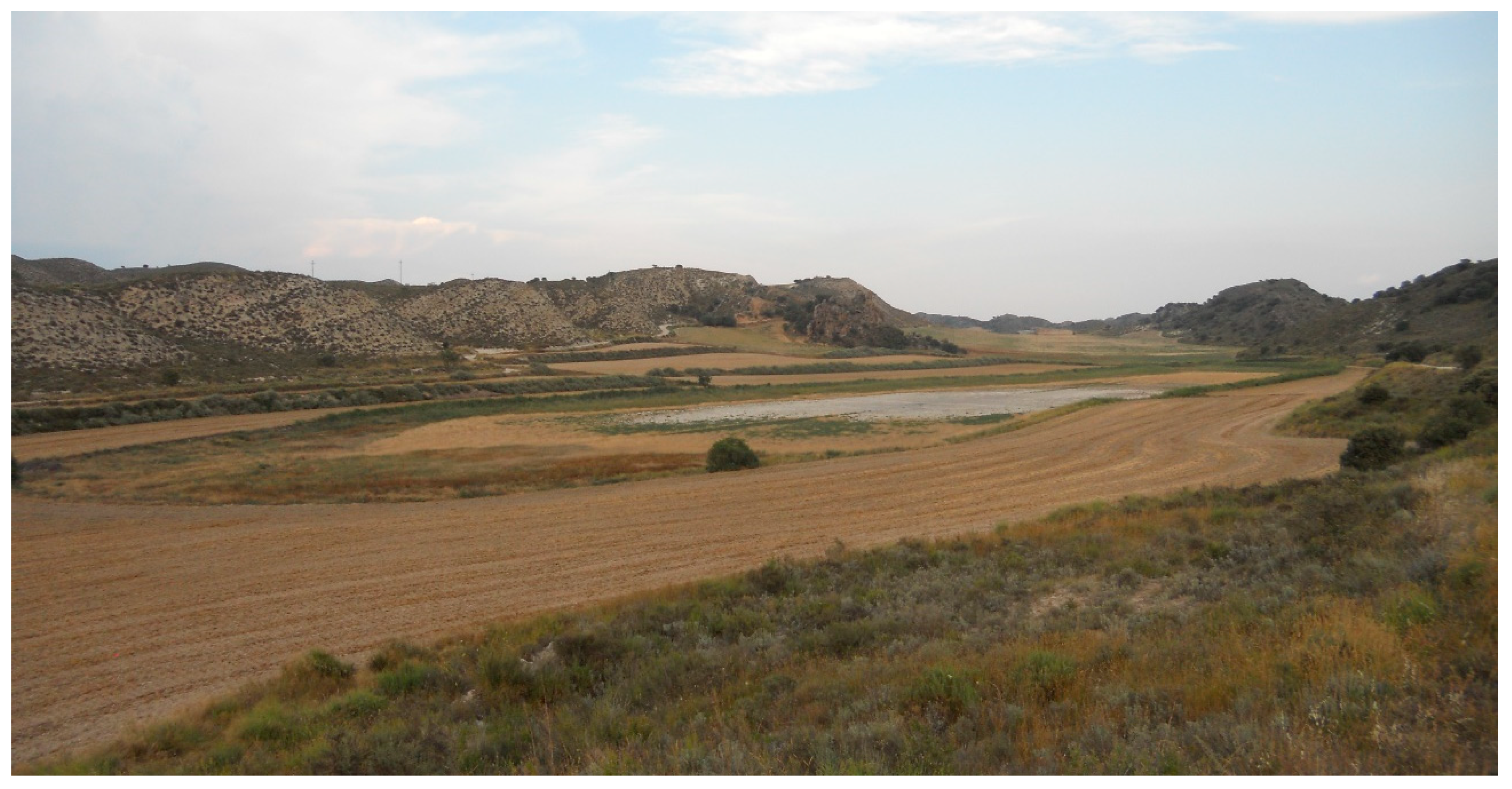
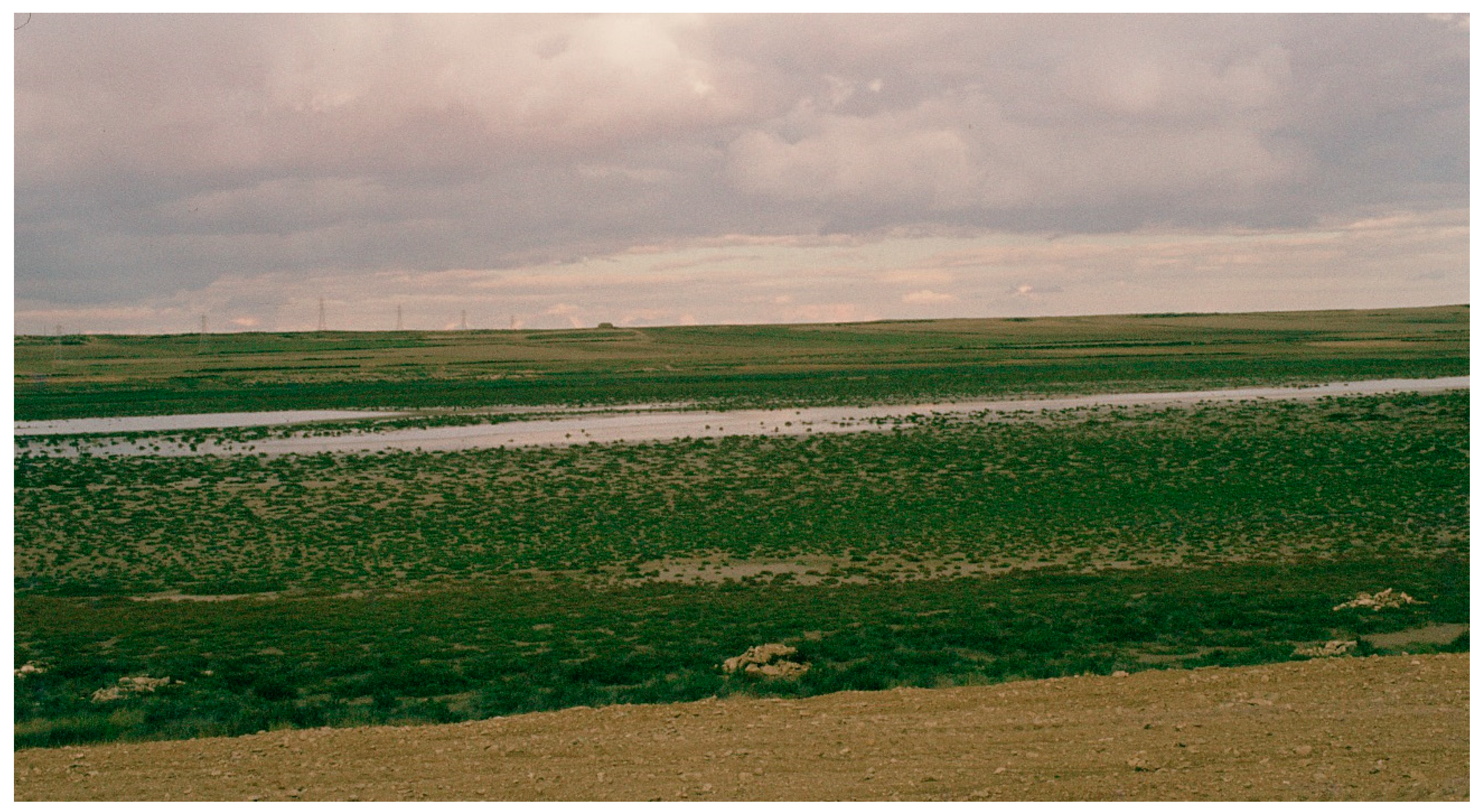
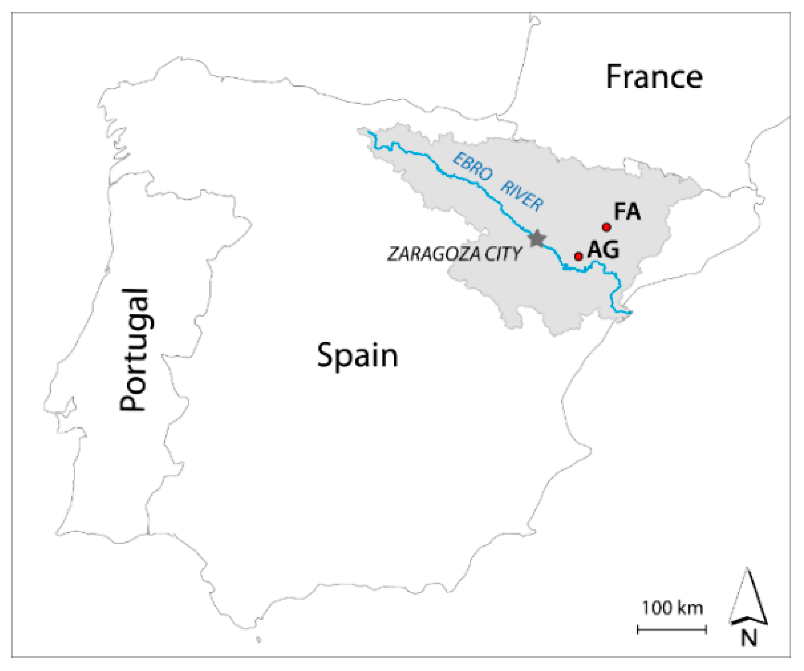
2.1. The Context of the Wetlands Studied

We compare the isolated wetland Farrachuela (FA) to Agustín (AG) which belongs to the Sástago-Bujaraloz complex. The two hypersaline wetlands lie about 70 km apart (Figure 1), and both of them occupy Quaternary depressions formed by dissolution of rocks rich in gypsum and more soluble salts, with the remaining residuum in their bottoms. A conspicuous network of surficial cracks appearing after each rain episode demonstrates the inundation, while the fresh plant residues visible to the naked eye evidence the recent biological activity in the soil. Contrariwise, the microcrystalline gypsum, i.e., the flour-like gypsum described elsewhere [4], is not observed within the two saladas studied, but does occur in the areas surrounding them. This fact mirrors the contrasting soil hydric regime of the almost permanently dry soils in the Central Ebro Basin against the persistently moist or wet soils in the enclaved saladas.

The two saladas occupy flat-bottomed valleys, which allows for preferential water circulation and accumulation. FA stands isolated in the landscape at the outcrops of the Barbastro Gypsum Formation from the Eocene–Oligocene age [16], whose dipping strata facilitate deep percolation of rainfall. AG is part of the largest group of saline wetlands in the Ebro Basin, with a total of 149 after the inventory of [17], a number that is in stark contrast with the absence of wetlands around FA. The near-horizontal Miocene strata of gypsum and limestone interbedded with lutites of the Bujaraloz Formation in Monegros [18] allow the occurrence of karstic depressions aligned along flat-bottomed valleys and low-lying areas hosting wetlands. Other differentiating factors are the presence of shallow saline aquifers (aquitards) in Monegros [19], responsible for groundwater discharge into the intermittently flooded depressions, and the wind regime that influences the excavation and shaping of the playa lakes in this area.

Winter cereals were cultivated in the watersheds of both saladas (Figure A1 and Figure A2 in the Appendix A) at the time of the samplings, i.e., July 2013 for Farrachuela; and February, March, April, July, and August of the years 1979–1980 and 1999–2000 for Agustín. The plants collected (

Table 1. Plants collected in Farrachuela [20] and in Agustín [21].

Farrachuela, 1981	Agustín, 2004 to 2007
Hornungia procumbens (L.) Hayek	Aeluropus littoralis (Gouan) Parl.
Helianthemum salicifolium (L.) Mill.	Artemisia herba-alba Asso
Frankenia pulverulenta L.	Arthrocnemum macrostachyum (Moric.) Moris in Moris and Delponte
Lepidium subulatum L.	Atriplex halimus L.
Phragmites australis (Cav.) Trin. ex Steud.	Frankenia pulverulenta L.
	Gypsophila struthium subsp. hispánica (Willk.) G. López
Farrachuela, 2013	Hordeum marinum Huds.
Suaeda spicata (Willd.) Moq.	Kochia prostrata = Bassia prostrata (L.) Beck in Rchb.
Salsola soda L.	Limonium sp. pl.
Puccinellia festuciformis (Host) Parl.	Puccinellia fasciculata (Torrey) E.P. Bicknell
Frankenia pulverulenta L.	Salsola vermiculata L.
	Suaeda vera subsp. braun-blanquetii Castrov. and Pedrol

) are well known as salinity and waterlogging tolerant or as gypsophilous, and they illustrate the ecology of these wetlands. The floristic composition has remained stable up to the present.

The aerial photographs from 1956 of both saladas attest that irrelevant anthropic interventions occurred prior to the years of the soil samplings presented in this study. We deem AG representative of those saladas of Sástago-Bujaraloz that remained in an acceptable state of conservation, even threatened by flooding with fresh water from forthcoming irrigation. The land around FA, cleared more than two hundred years ago, bears barley and sparse olive trees, with no irrigation planned.

2.2. Climate

Climate data were obtained from the nearest automatic weather stations, in Tamarite, located 11.5 km south of Farrachuela, and Valfarta located 8.5 km NNW of Agustín. Both stations belong to the Spanish SIAR network. For the period 2004–2021, the mean annual rainfall in the Farrachuela area was 350 mm, the mean temperature was 14 °C, and the mean evapotranspiration rate was 1041 mm. The same mean temperature and precipitation of 359 mm were obtained in Agustín area for the same period, with a higher mean evapotranspiration rate (1258 mm).

Using the terminology of the Soil Survey Staff [22] and the data from the two weather observatories, the soil moisture regime at both saladas is aquic and the most likely soil temperature regimes are mesic for Farrachuela and thermic for Agustín.

2.3. Sampling

We collected soil samples by hand augering down to a depth of 2 m in Farrachuela, and until reaching an impenetrable layer in Agustín. All the samples were examined visually, including with a magnifying glass, and by touch both in the field and in the laboratory. Then, the samples were air-dried and passed through a 2 mm sieving mill to obtain the fine earth fraction, i.e., <2 mm Ø, used for further analyses.

Table 2. Location and size of the two wetlands and data of their sampling.

Name of the Salada	Farrachuela	Agustín
Sheet name of the National Topographic Map of Spain at 1:25 000 scale	Tamarite	Bujaraloz
Geographical coordinates (N, E)	41.8845, 0.3742	41.4311, −0.1091
Surface area, ha	3.4	68.1
Elevation, meters above sea level	400	329
Number of augerings	4	24
Augering mean deep, cm	200	63
Number of soil samples for chemical analyses	32	133

shows details of the augerings, and the number of analyses.

2.4. Analyses

The official methods of the Agricultural Ministry of Spain [23] provided the methodology for the chemical determinations. Calcium carbonate (CaCO₃) equivalent (CCE) was measured by gasometry, and gypsum was titrated as per [24].

All the determinations of electrical conductivity are reported as dS m⁻¹ at 25 °C. We measured the electrical conductivity (EC1:5) of the aqueous extracts at an earth-to-water ratio weight:weight of 1:5. Moreover, we prepared water-saturated pastes of the fine earth [25], recording the water saturation percentage (SP, %) and measuring the electrical conductivity of the extract (ECe), and its pH (pHe). The major ions in the saturation extracts were determined using the classical methods specified in [20].

We report the ionic contents (ionic-C, mmolc L⁻¹) as the sum of cations + anions divided by two in order to counterbalance the deviations to electroneutrality, frequent when analyzing highly concentrated solutions. The sodium adsorption ratio SAR (mmolc L⁻¹)^0.5 is calculated from the concentrations in mmolc L⁻¹ of Na⁺, Ca²⁺, and Mg²⁺ by the expression SAR = Na⁺/[(Ca²⁺ + Mg²⁺)/2]^0.5.

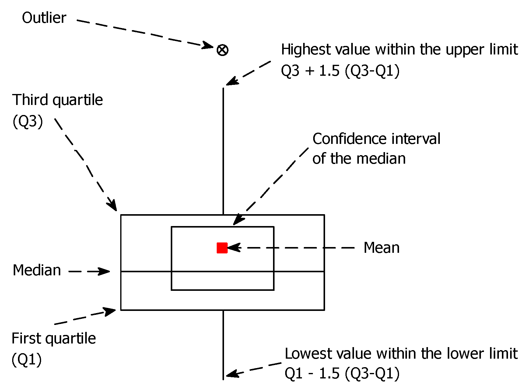
2.5. Statistical Procedures

We display and analyze most of our data through graphical methods, representing the measures of exploratory data analysis by means of the intuitive boxplots proposed by [26]. Our boxplots, drawn following [27], include the 95% confidence intervals for the medians estimated as per [28]. Figure A3 in Appendix A sketches the meanings of all the parts of the boxplot diagrams presented in this paper.

We calculate the regression lines by the Ordinary Least Squares (OLS) method with p = 0.05, and we check their equations with a non-parametric simple regression using Theil’s method [29,30] in order to cope with the habitual non-Gaussian distributions of our data, the frequent outliers, and the limited effectiveness of some data batches.

3. Results and Discussion

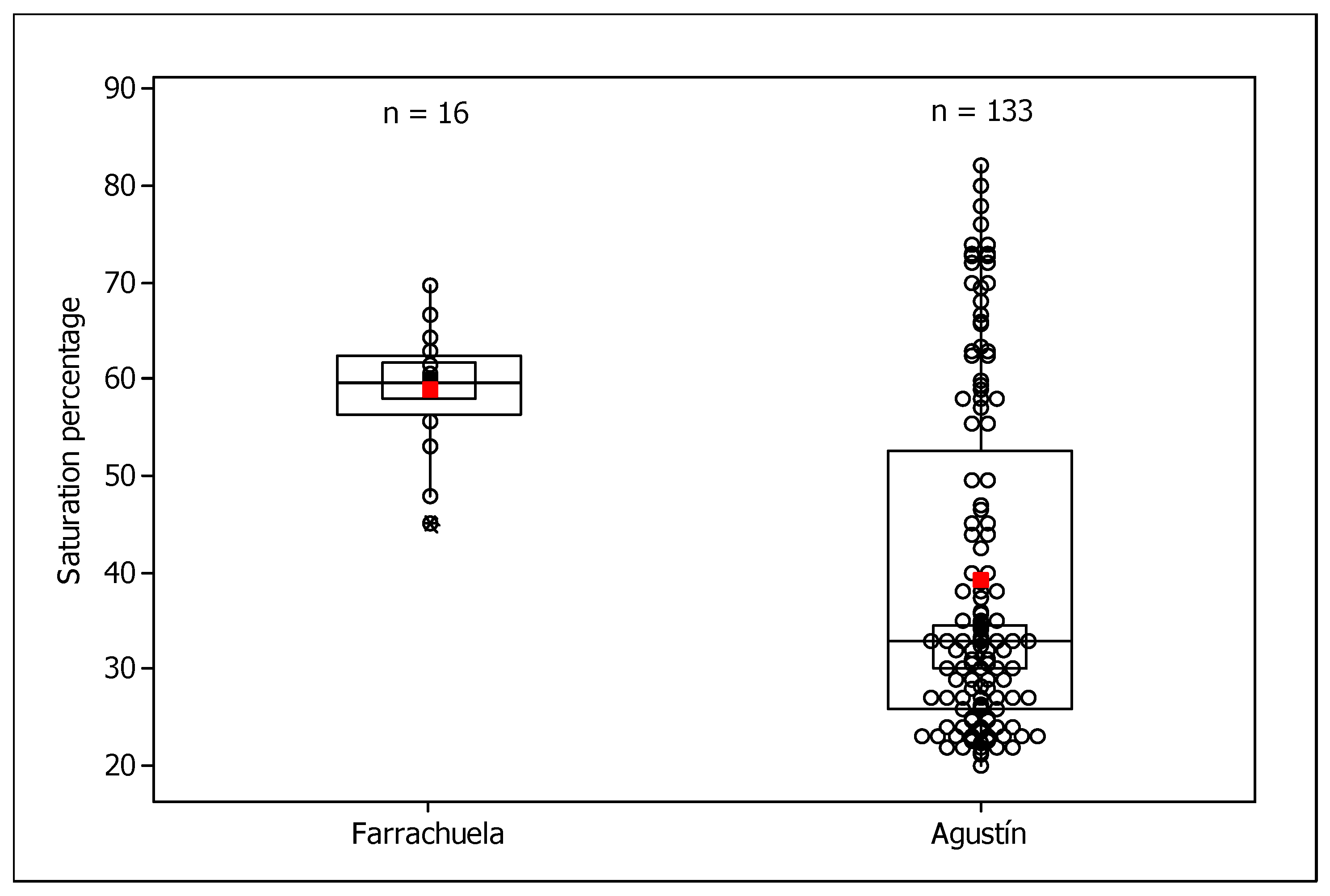
3.1. Saturation Percentages

The mean SP in the 16 samples from FA with this determination is 59.0%, far from the 39.3% in the 133 samples from AG. The other statistics and the distributions of SP also are very distinct between the two saladas (Figure 2). The use of SP to compare soil characteristics is sounder than the classical particle size distribution (PSD) determinations, which, in some materials, produce artifactual results, as argued in Section 3.9.

The saturated paste extraction approximates the field capacity of the soil much better than other, more diluted, soil-to-water ratios, while making water extraction feasible with simple equipment [31,32]. Thus, the extract of the saturated paste is broadly used [22,23,25] to assess the salt tolerance of plants by measuring the electrical conductivity of the extract (ECe). Also, eventually, its ionic composition is determined to appraise the effects of individual ions or their co-occurrence, as is the case of the structural stability of the soil. Many studies of soil salinity report SP because of its interest in understanding the hydric behavior of the soil. The simplicity of the preparation of the saturated paste, based on the skill of the operator, and the saturation point determined by feel and experience, together with the use of few―if any―sophisticated laboratory tools, probably contribute to SP being overlooked in some studies.

However, even if the composition of saturated extracts was not to be analyzed, the SP is worth recording because SP can be a surrogate for textural composition, or “a quantitative expression of soil texture” as noted by [33], and represents key functional soil properties, like the available water capacity [34]. This is an old issue in soil science when “dealing with single-valued expressions instead of trying to interpret the complex series of numbers represented by the mechanical analysis” [35], as in the class–moisture equivalent diagram of [36]. When dealing with soil salinity, SP has been used in recent attempts [37] at estimating ECe from extracts at fixed dilution ratios. Also, SP is a relevant soil characteristic for precision agriculture, as noted in [38], with SP performing better than organic matter, CaCO₃, ECe, and pH for yield prediction. Furthermore, SP can help to check consistency over time in sample preparation [32], which we also did successfully to compare two operators [39].

The surrogate role of SP for texture is especially useful in gypsum-rich soils where the standard methods for PSD determination are unsuitable [4,40] and many substitute methods are unfeasible in routine labs. In [8], hand textural class estimates were used to check the proposed method for PSD determination. After the above considerations, we did not determine PSD, and we claim SP as a strong indicator of hydric behavior and a reliable surrogate for textural composition [40,41,42].

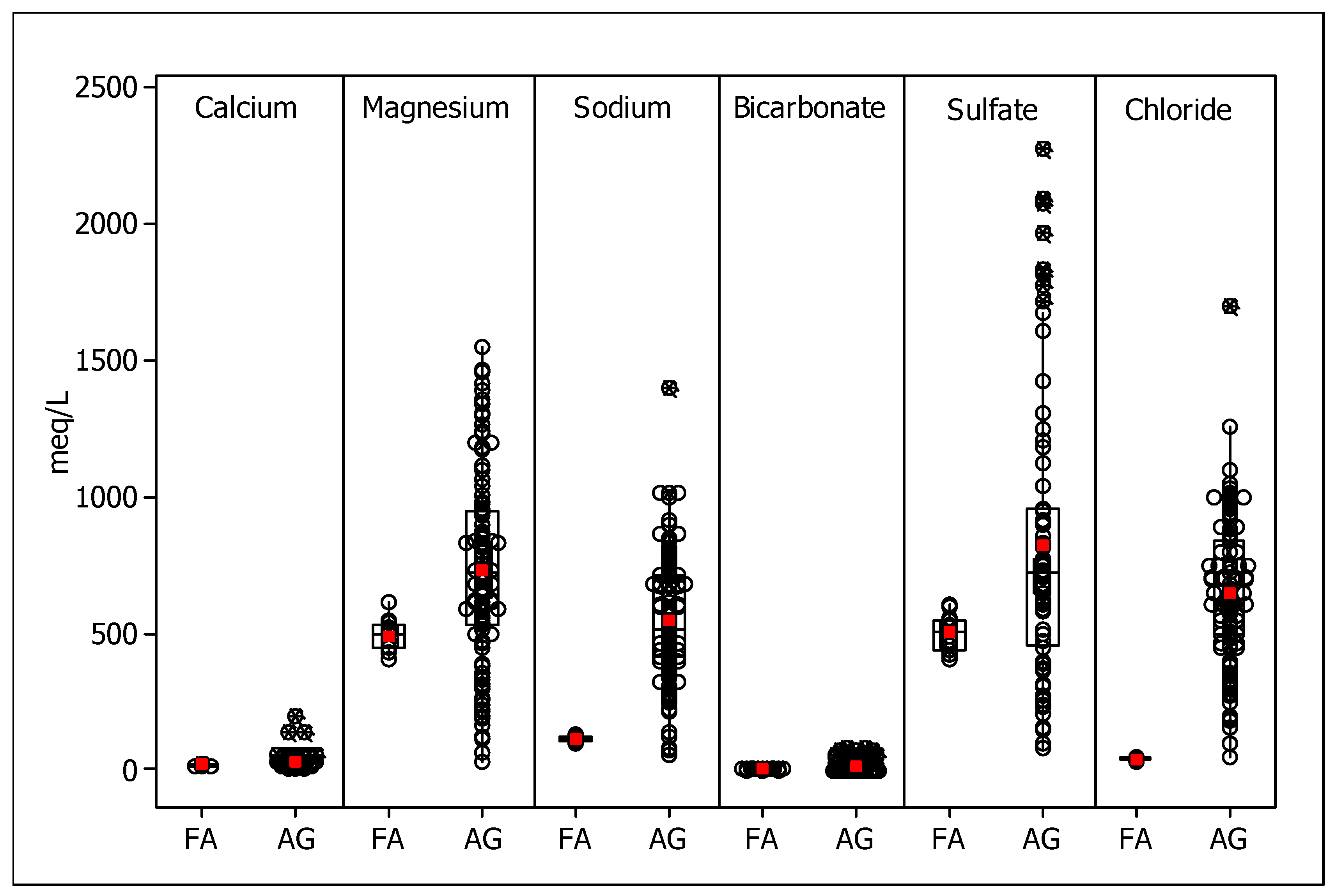
3.2. Major Mineral Components

The boxplots of calcium carbonate equivalent (CCE) and gypsum for each salada (Figure 3) show their distribution along the samples, and the prominence of both components. The mean percent rounded to the nearest integer for FA and AG are 24% and 10% for CCE while for gypsum they are 30% and 62%, respectively. Then, the remaining material, i.e., silica and silicates―including the mineralogical clays―plus organic components is <50% on average. These compositions agree with the contrasting average SP of 59% in FA, and 39% in AG (Figure 2), since gypsum and calcium carbonate have a much lower water-holding capacity than the other minority components, like clay and organic matter.

The abundance of gypsum in the soils and geological materials governs the chemistry of the soil solution and the exchange complex due to their saturation in Ca²⁺. The contents of gypsum (Figure 3) in the samples analyzed―with a minimum of 12.2% in FA and 9.5% in AG―largely guarantee Ca²⁺ saturation, preventing clay dispersion.

3.3. Soil Salinity

In the present study, a common visual symptom of soil salinity is the white bright efflorescences mostly produced by evapoconcentration during dry periods at the bottoms and margins of both FA and AG. These efflorescences are often composed mainly of crystals of gypsum and more soluble salts, as evidenced in the field by naked-eye and hand-lens observations, as well as by taste. The halophilous vegetation also attests the soil salinity.

The visual symptoms do not quantify the salt stock in the soils. Such stock is a key indicator of the ecological status of the soil, which can be tracked by recording the changes in the salt content through time. To establish this stock, the soil salt must be extracted at fixed-ratio dilution, higher than the saturated paste [25,31] as is evident for hypersaline soils [43]. To appraise the salt stock of the soil, we use the easy, unsophisticated, and reproducible determinations of EC1:5 [25]. Such attributes make EC1:5 well-suited for future comparative assessments.

The mean of EC1:5 in 32 extracts of FA was 7.18 dS m⁻¹, versus 8.78 dS m⁻¹ in the 72 extracts from AG for which EC1:5 was analyzed (Figure 4). We consider these conductivities a proxy for the total content of highly soluble salts that can allow tracking the evolution of the soil’s salt stock. The 1.68 dS m⁻¹ of the difference between the means of EC1:5 seems moderate. However, AG is a more salt-stressing environment than FA, as shown by the vegetation (Table 1) and by the mean ECe of 37.04 dS m⁻¹ for FA against 68.58 dS m⁻¹ for AG. The difference is more pronounced than in EC1:5, and the same is true for the other statistics graphed in Figure 4. The longer range of the distributions in AG seems sound if considering the 20-fold surface area of AG versus FA (Table 2), which allows for more variable conditions in AG.

The much higher values of EC1:5 and ECe in AG than in FA (Figure 4) agree with the species of halophytes recorded at both saladas (Table 1). The absence of Arthrocnemum macrostachyum in FA is relevant because this plant lives in the more often inundated areas of AG where ECe is >80 dS m⁻¹, a soil salinity not reached in FA. The difference is also pronounced if only the upper soil layer is considered, with about 37 dS m⁻¹ in FA versus 85 dS m⁻¹ in AG. Accordingly, A. macrostachyum, the most salinity perennial tolerant plant, lives in AG and not in FA.

The scatterplot of ECe on EC1:5 (Figure 5) does not show the inflection associated with gypsum [43] because all samples have EC > 2.25 dS m⁻¹ in both EC1:5 and ECe. The wide scattering of the values―seen in the plot―hampers the estimation of ECe from the plain EC1:5. If desired, estimates of ECe can be made from EC1:5 by the method in [44]. In this article, we apply the easy transformation of EC1:5 by SP as per [45], i.e., by calculating regressions of the shape ECe = a + b × EC1:5 × (500/SP)^q with empirical powers of q. The best correlation coefficients (

Table A1. Pearson’s correlation coefficients (R) obtained with OLS regression equations of the shape ECe = a + b × EC1:5 × (500/SP)^q for several arbitrary values of q.

	Farrachuela	Agustín
q	R
0	0.291	0.360
0.50	0.862	0.887
0.55	0.863	0.902
0.60	0.857	0.913
0.65	0.848	0.920
0.70	0.837	0.925
0.80	0.812	0.928
0.90	0.787	0.925
1	0.763	0.919

, in Appendix A) were 0.863 for FA, and 0.928 for AG.

For the present article, the equations allowed us to check the coherence between ECe and EC1:5. The future studies of these wetlands will have to decide whether or not to estimate ECe from EC1:5 with this kind of equation. The reason is that ECe is the standard indicator of saline stress on plants, used to express a plant’s tolerance to soil salinity, a key feature for crop feasibility [32]. The equations in Table A1 allowed us to check the consistency between ECe and EC1:5 and will help to decide in future studies of these wetlands whether or not to estimate ECe from EC1:5 with these kinds of equations.

3.4. Soil Classification

The inspection of the auger samples and their analyses for ECe and gypsum content enabled us to identify the diagnostic horizons defined by the Soil Survey Staff [22] without the need to open a trench, a much more soil disturbing procedure. According to the data of the ECe and gypsum content, and following step-by-step the statements in [22], the soils of FA and AG have the Salic and Gypsic horizon in conjunction. Thus, the soils of both wetlands are Gypsic Aquisalids.

3.5. Ionic Contents of the Saturation Extracts

Bicarbonate, titrated in all the extracts, was always below the limits of detection. Potassium contents are irrelevant. The pairs of boxplot diagrams in Figure 6 compare the content of each of the ions Ca²⁺, Mg²⁺, Na⁺, HCO₃⁻, SO₄²⁻, and Cl⁻ in the saturation extracts of FA to AG. The range of all the distributions is broader for AG, which also happens for the interquartile ranges.

Of note are: (i) the greater surface area of AG and the greater number of samples than in FA, and (ii) the greater surface area of AG allowing for more diverse hydric conditions including the redistribution of water by the wind. These conditions are mirrored by the occurrence of the highly halophilic A. macrostachyum in AG. Both saladas are similar with regard to the predominance of SO₄²⁻ and Mg²⁺, but the concentrations of Cl⁻ and Na⁺ are significantly lower in Farrachuela, hence its lower salinity.

Figure 6 shows that the median concentrations are significantly lower in FA than in AG for the six ions in question, but the difference is insignificant for sulfate. The mean concentrations are also lower in FA than in AG for the ions analyzed. This happens when computing all the analyses from AG extracts (Figure 6), and also if computing only the extracts with the six ions analyzed (

Table 3. Mean contents (mmolc L⁻¹) of six major ions for: (a) the 16 saturation extracts from FA, (b) all the analytical determinations from AG as shown in Figure 6, (c) differences between these means, (d) means of the 76 extracts from AG with the six ions titrated, and (e) differences between the means of all determinations from AG and the means of FA.

	Ca2+	Mg2+	Na+	Cl−	SO42−	HCO3−
		mmolc L−1
(a) Farrachuela	18.9	492.3	113.0	40.7	503.1	2.2
(b) all determinations from Agustín *	29.0	734.0	546.4	646.4	820.6	16.7
(c) differences between saladas, (b) minus (a)	10.1	241.7	433.4	605.7	317.5	14.5
(d) Agustín, only the 76 samples with the six ions titrated	27.5	716.7	523.4	634.5	820.6	3.0
(e) differences, b minus d	1.5	17.3	23.0	11.9	---	13.7

* The number of determinations in AG were 132 for Ca²⁺, Na⁺, and Cl⁻; 124 for Mg²⁺; and 76 for SO₄²⁻.

). This Table also shows numerically the differences between the mean contents of each individual ion in the two saladas. The greatest difference occurs in Cl⁻, followed by Na⁺ and SO₄²⁻, and then by Mg²⁺, with 594, 410, 317, and 224 mmolc L⁻¹, respectively. We deem irrelevant the differences in Ca²⁺ and HCO₃⁻. The differences between the two wetlands for Mg²⁺, Na⁺, SO₄²⁻, and Cl⁻ agree with their distinct physical characteristics outlined in the second paragraph of Section 2.1. Of note is the detection of magnesium by taste in the efflorescences of AG, agreeing with the boxplot in Figure 6. The abundance of magnesium should be due to evapoconcentration from the parental rocks of gypsum that contain this element.

Table 3 also shows the consistency of the results obtained by computing all the available titrations or only the ones from the samples with the six ions analyzed. This feature is interesting for long-term tracking, when the homogeneity of the number of ions analyzed along successive campaigns cannot be guaranteed.

3.6. SAR and pH

Due to their salinity and frequent inundation, the saladas are either bald or seasonally populated by halophytes, and are unusable for the cash crops feasible in the Ebro Basin. Notwithstanding, we present (

Table 4. Statistics of SAR and pH in the saturation extracts of samples from Farrachuela (FA) and Agustín (AG).

	Number of Analyzed Samples	Minimum	Maximum	Median	95% Confidence Interval for The Median
		SAR (mmolc/L)0.5
FA	16	6.70	7.80	7.00	6.80	7.30
AG	124	10.41	45.08	27.96	26.80	28.94
		pH
FA	16	7.92	8.44	8.26	8.17	8.36
AG	52	7.28	8.33	7.92	7.71	8.00

) the statistics of SAR and pH of the saturation extracts in both wetlands, showing their significant difference. The values of SAR in Farrachuela are well below the classical threshold of SAR = 13 for clay dispersion in soils. By contrast, the values of SAR in Agustín are largely in excess of 13, denoting the unfeasibility of cash crops. The pH values are significantly different between the two wetlands (Table 4); however, pH by itself should not be a problem for most plants, as it ranges from 7.28 to 8.44 in the two saladas. These basic pH values are allowable for most plants. For the infiltration behavior, SAR must be considered jointly with pH and salinity [45].

For SAR, it does not make sense to apply the commonly used threshold SAR < 13 (mmol_c L⁻¹)^0.5 to judge the sustainability of irrigation, since for most soil samples the ECe is >>20 dS m⁻¹ (Table 4). Then, the SAR/EC ratios do not affect the clay dispersion and no associated imperviousness would happen [45,46]. Moreover, the contents of mineralogical clay are low, as the sum of the means of gypsum and calcium carbonate equivalent are 54% for Farrachuela, and 72% for Agustín. The mineralogical clays are thus in the minority, reducing the value of SAR to predict the hydrological behavior of these gypsum-rich soils often saturated in water. More relevant to the hydraulic behavior is the horizontal microstructure in FA and AG, similar to the layering described in other saladas in Monegros.

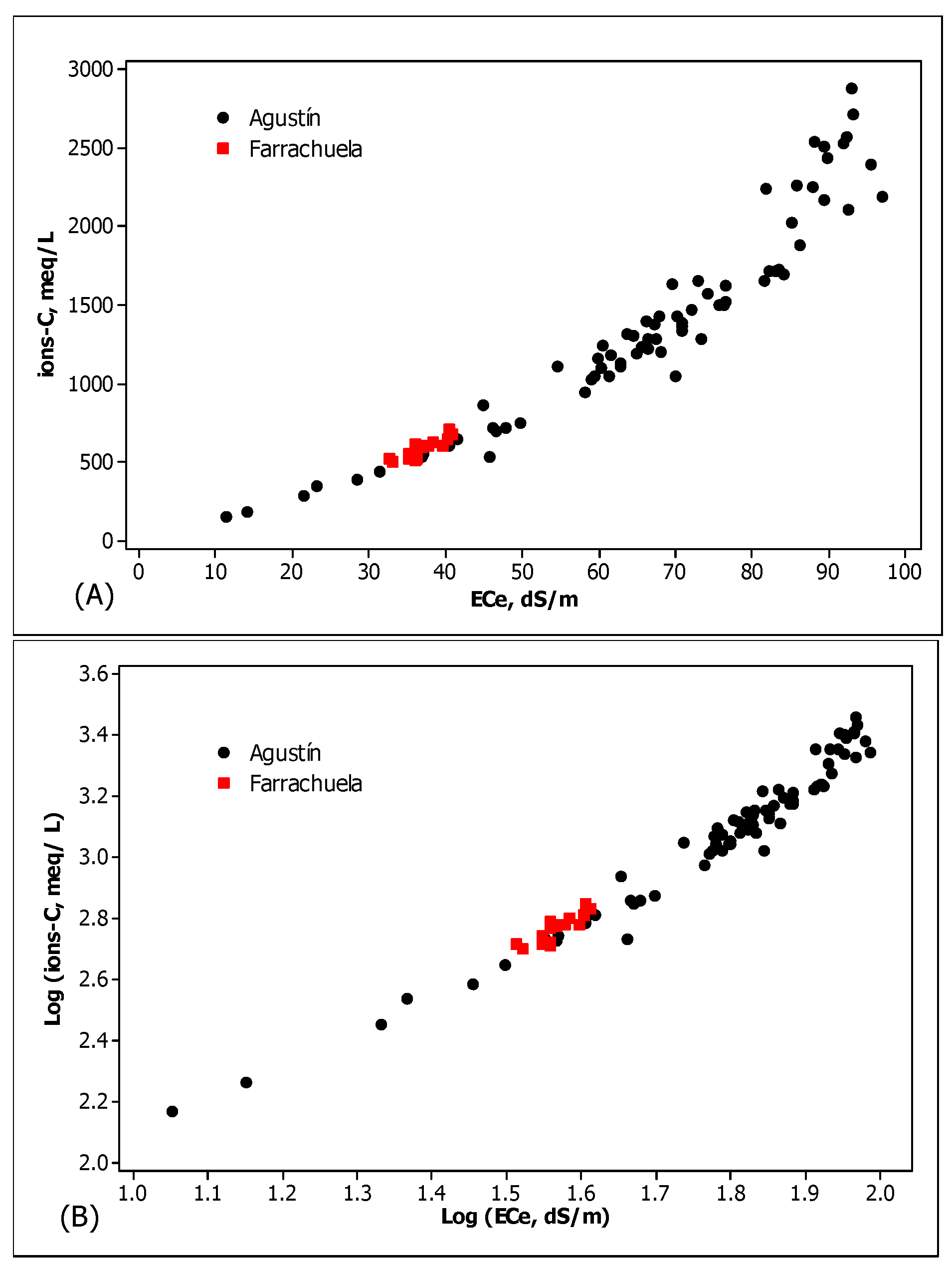
3.7. Relationship between Ionic Concentration and ECe

Figure 7A shows the concordance between both saladas regarding the relation of ionic contents (ionic-C, mmolc L⁻¹) in the extracts, as defined in Section 2.4., versus ECe. The tusk-shaped distribution in this figure illustrates the increase in the ratio of ions to ECe for the high ionic concentrations, due to the occurrence of neutral and other ionic pairs [47]. The dilution of the more concentrated extracts, required for the analytical methods, also contributes to the scattering of values in the high concentrations.

For the two saladas, the distributions approach a straight line after transforming both variables using decimal logarithms (Figure 7B), as proposed in [48]. This reinforces the consistency of the data.

Table A2. Regression equations of the shape log ionic-C = a + b × log ECe calculated by OLS and Theil methods for 16 and 76 soil samples from Farrachuela and Agustín, respectively.

Salada	Method	a	b	R2, %
Farrachuela	OLS	0.659	1.34	75.4
	Theil	0.701	1.32	75.4
Agustín	OLS	0.541	1.42	95.5
	Theil	0.302	1.54	95.5

in the Appendix A shows the regression equations obtained from these transformations.

3.8. Relationship between the Concentration of Individual Ions and ECe

The saturation extracts of AG showed a good correlation coefficient (R) of the ions between them as well as between the ECe and the ions (

Table 5. Correlation coefficients between ECe and the main ions, and between them. The p-value is < 0.001, except if non-significance (n.s.) is indicated.

	ECe	Mg2+	Na+	SO42−
		Farrachuela
Mg2+	0.822
Na+	0.792	0.815
SO42−	0.815	0.840	n.s.
Cl−	n.s.	n.s.	n.s.	n.s.
		Agustín
Mg2+	0.913
Na+	0.936	0.901
SO42−	0.794	0.907	0.792
Cl−	0.945	0.888	0.957	0.723

). These coefficients in AG are higher than their counterparts in FA, except the correlation of ECe with SO₄²⁻, which is slightly higher in FA than in AG.

For the saturation extracts of FA, the correlation of ECe was significant (p < 0.001) with Mg²⁺, Na⁺, and SO₄²⁻, but not with Cl⁻. By contrast, in AG the correlation ECe/Cl⁻ was the highest, as shown in Table 5.

The coefficients of determination (R²) attained by the OLS regression of the average ionic content versus ECe (Table 5) are the same as when using Theil calculations, while the standard errors using the OLS regression are smaller than with Theil regressions. The OLS method is thus recommended for estimating the ionic content from the ECe in the saturation extracts of both saladas within the ranges indicated in

Table 6. Regression equations of the shape “ionic-C = a + b × ECe” with the coefficient of determination (R², %) and standard error (S) calculated for 16 and 76 soil samples from Farrachuela and Agustín, respectively. The methods of calculation are ordinary least squares (OLS), and Theil using the median of the interceptors.

	Method	a	b	R2	S	Range of Ionic-C
				%	mmolc L−1
Farrachuela	OLS	−213.1	21.59	76.2	29.60	502.4 to 705.2
	Theil	−200.4	21.33	76.2	32.71
Agustín	OLS	−620.6	30.30	88.8	218.8	147.8 to 2876.0
	Theil	−629.6	29.50	88.8	281.1

. These equations could help to streamline the environmental tracking of the saladas.

3.9. The Specificity in the Analytics of Gypseous Materials

In fresh soil samples of the gypseous horizons of the soils studied, the abundant gypsum crystals are bound together by fine material, the strength of which increases as the moisture content decreases. This is a well-known characteristic of many soils [49]. The coarse gypsum crystals are easily separated, intact, using the fingers when the sample is wet, but when air dried, these crystals break easily —mostly along cleavage plains— before becoming detached from the mass. The breaking happens even if a dry soil sample is gently crushed between a wooden board and a wooden rolling pin, and, of course, in mechanical shakers and sieving mills, until they eventually pass through the sieve. Milling may result in the entire sample passing through the 2mm sieve, making the time at which the operation is interrupted arbitrary. For this reason, the content of coarse gypsum crystals and other gypsum fragments must be appraised before drying and sieving in the lab.

In gypsum-rich soils, the low hardness and cohesion of the gypsum crystals lessens the value and significance of the particle size separates obtained after milling. Moreover, the abundance of gypsum and its solubility (≈2.4 g L⁻¹) immediately cause the sedimentation of clays when being dispersed for particle size separations [4,8]. The judgments about other methods for PSD determinations based on X–ray fluorescence, e.g., [50] or its combination with FT-NIR spectroscopy, e.g., [51], or with Vis-NIR and pXRF [52] are unsound if these methods are calibrated against either pipette or wet sieving and hydrometer, which do not work in gypseous soils. The method proposed by [8], based on sonication in a 7:3 ethanol to water solution―a procedure available in few labs―allows dispersion of fine earth, but the significance of the coarse and fine earth remains arguable in the soils studied. In the common circumstances of gypsum-rich soils, the lab determination of PSD should not be taken as representing the behavior of the undisturbed soil. These shortcomings led to coining two terms in lieu of texture: “Coarse Gypsum Material” and “Fine Gypsum Material” [49].

The issues discussed in the above two paragraphs indicate the non-sense of using some routine analytical methods with gypseous sediments and soils. Then, [4] proposed the elimination of PSD for assessing the hydric behavior of gypseous soils. Specifically, we support considering saturation percentage as a sound and useful surrogate for textural composition. Accordingly, we did not separate the clay fraction, whose determination would also be impractical, cumbersome and probably irrelevant for future monitoring.

4. Conclusions

The article provides a snapshot of the main limiters to life in two inland saline marshes. We hope it provides a baseline for protecting of these shelters of biodiversity. The intuitive graphical procedures used in this article allow for a quick and detailed statistical comparison of the soil characteristics that are decisive for life in the saline wetlands studied. The features compared are: (i) contents of gypsum and calcium carbonate; (ii) soil salinity as EC1:5; (iii) saturation percentage; and (iv) pH, electrical conductivity and ionic contents in the saturation extracts. The data will constitute a baseline —the only one at present— for tracking possible compositional changes in the two saladas studied. The calculation methods and graphical presentation are easily transposable to other saline wetlands, and may allow for multiple comparisons in the future.

The characteristics studied herein ought to be contrasted with other saline wetlands in order to delimit the environmental conditions for the life of specific plants, microbes, or other organisms. Hopefully, the correlations presented in this article will support the management and conservation measures to be implemented by environmental authorities in charge of the wetlands.

In situ recording of variable soil parameters is advisable. For some of them, the technology is available and is continuously improving. However, the implementation of recording seems unlikely in the near future due to the limited capacity of the conservation agencies responsible.

The misuse of analytical techniques that are wrong or unsound for gypsum-rich soils, like the ones discussed in the present article, is a key point to be: (i) avoided when conducting future analyses, and (ii) checked when scrutinizing heritage data.

References

1. Cížková, E.; Navrátilová, J.; Martinát, S.; Navrátil, J.; Frazier, R.J. Impact of water level on species quantity and composition grown from the soil seed bank of the inland salt marsh: An ex-situ experiment. Land 2020, 9, 533. [Google Scholar] [CrossRef]
2. Domínguez-Beisiegel, M.; Herrero, J.; Castañeda, C. Saline wetlands’ fate in inland deserts: An example of 80 years’ decline in Monegros, Spain. Land Degrad. Dev. 2013, 24, 250–265. [Google Scholar] [CrossRef]
3. Köninger, J.; Panagos, P.; Jones, A.; Briones, M.J.I.; Orgiazzi, A. In defence of soil biodiversity: Towards an inclusive protection in the European Union. Biol. Conserv. 2022, 268, 109475. [Google Scholar] [CrossRef]
4. Casby-Horton, S.; Herrero, J.; Rolong, N.A. Gypsum soils—Their morphology, classification, function, and landscapes. Adv. Agron. 2015, 130, 231–290. [Google Scholar] [CrossRef]
5. Goryachkin, S.V.; Spiridonova, I.A.; Sedov, S.N.; Targulian, V.O. Boreal soils on hard gypsum rocks: Morphology, properties, and genesis. Eurasian Soil Sci. 2003, 36, 691–703. [Google Scholar]
6. Tuyukina, T.Y. Geochemical studies of northern taiga (gypsum) karst ecosystems and their high vulnerability to natural and anthropogenic hazards. Environ. Geol. 2009, 58, 269–274. [Google Scholar] [CrossRef]
7. Palacio, S.; Cera, A.; Escudero, A.; Luzuriaga, A.L.; Sánchez, A.M.; Mota, J.F.; Pérez-Serrano, M.; Merlo, M.E.; Martínez-Hernández, F.; Salmerón-Sánchez, E.; et al. Recent and ancient evolutionary events shaped plant elemental composition of edaphic endemics: A phylogeny-wide analysis of Iberian gypsum plants. New Phytol. 2022, 235, 2406–2423. [Google Scholar] [CrossRef]
8. Pearson, M.J.; Monteith, S.E.; Ferguson, R.R.; Hallmark, C.T.; Hudnall, W.H.; Monger, H.C.; Reinsch, T.G.; West, L.T. A method to determine particle size distribution in soils with gypsum. Geoderma 2015, 237–238, 318–324. [Google Scholar] [CrossRef]
9. Heino, J.; Alahuhta, J.; Bini, L.M.; Cai, Y.; Heiskanen, A.S.; Hellsten, S.; Kortelainen, P.; Kotamaki, N.; Tolonen, K.T.; Vihervaara, P.; et al. Lakes in the era of global change: Moving beyond single-lake thinking in maintaining biodiversity and ecosystem services. Biol. Rev. 2021, 96, 89–106. [Google Scholar] [CrossRef]
10. Lehner, B.; Doll, P. Development and validation of a global database of lakes, reservoirs and wetlands. J. Hydrol. 2004, 296, 1–22. [Google Scholar] [CrossRef]
11. Prăvălie, R.; Sîrodoev, I.; Ruiz-Arias, J.; Dumitraşcu, M. Using renewable (solar) energy as a sustainable management pathway of lands highly sensitive to degradation in Romania. A countrywide analysis based on ex-ploring the geographical and technical solar potentials. Renew. Energy 2022, 193, 976–990. [Google Scholar] [CrossRef]
12. Wang, G.; Li, G.; Liu, Z. Wind farms dry surface soil in temporal and spatial variation. Sci. Total Environ. 2023, 857, 159293. [Google Scholar] [CrossRef]
13. Alberto, F.; Navas, A. La participación de los yesos en la salinización de las aguas superficiales de la cuenca del Ebro. I. Cartografía de síntesis de las formaciones con yesos. An. Aula Dei 1986, 18, 7–18. Available online: http://hdl.handle.net/10261/13516 (accessed on 3 September 2023).
14. Herrero, J.; Castañeda, C. A Dataset of Scientific References on Saline Wetlands of Monegros, NE Spain. Mendeley Data. 2023. Available online: https://data.mendeley.com/datasets/kxbgpc8y5r/3 (accessed on 20 September 2023).
15. Reid, R.P.; Oehlert, A.M.; Suosaari, E.P.; Demergasso, C.; Chong, G.; Escudero, L.V.; Piggot, A.M.; Lascu, I.; Palma, A.T. Electrical conductivity as a driver of biological and geological spatial heterogeneity in the Pu-quios, Salar de Llamara, Atacama Desert, Chile. Sci. Rep. 2021, 11, 12769. [Google Scholar] [CrossRef]
16. Pardo, G.; Villena, J. Aportación a la geología de la región de Barbastro. Acta Geol. Hisp. 1979, 14, 289–292. [Google Scholar]
17. Castañeda, C.; Herrero, J.; Conesa, J.A. Distribution, morphology and habitats of saline wetlands: A case study from Monegros. Geol. Acta 2013, 11, 371–388. [Google Scholar] [CrossRef]
18. Salvany, J.M.; García-Vera, M.A.; Samper, J. Geología e hidrogeología de la zona endorreica de Bujaraloz-Sástago (Los Monegros, provincias de Zaragoza y Huesca). Acta Geol. Hisp. 1995, 30, 31–51. [Google Scholar]
19. Samper-Calvete, F.J.; García-Vera, M.A. Inverse modeling of groundwater flow in the semiarid evaporitic closed basin of Los Monegros, Spain. Hydrogeol. J. 1998, 6, 33–49. [Google Scholar] [CrossRef]
20. Herrero, J.; Castañeda, C.; Velayos, M. Salada Farrachuela, a saline wetland in Tamarite de Litera, Spain. Bol. Real Soc. Esp. Hist. Nat. 2020, 114, 67–80. [Google Scholar] [CrossRef]
21. Conesa, J.A.; Castañeda, C.; Pedrol, J. Las saladas de Monegros y su entorno. In Hábitats y Paisaje Vegetal; Consejo de Protección de la Naturaleza de Aragón: Zaragoza, Spain, 2011; 540p, ISBN 978-84-89862-76-0. [Google Scholar]
22. Soil Survey Staff. Keys to Soil Taxonomy, 13th ed.; USDA-Natural Resources Conservation Service: Washington, DC, USA, 2022. [Google Scholar]
23. M.A.P.A. Métodos Oficiales de Análisis; Tomo III; Ministerio de Agricultura, Pesca y Alimentación, Secretaría General Técnica: Madrid, Spain, 1994; 662p. [Google Scholar]
24. Artieda, O.; Herrero, J.; Drohan, P.J. A refinement of the differential water loss method for gypsum deter-mination in soils. Soil Sci. Soc. Am. J. 2006, 70, 1932–1935. [Google Scholar] [CrossRef]
25. USDA; United States Salinity Laboratory Staff. Diagnosis and Improvement of Saline and Alkali Soils. Agriculture Handbook no. 60. Reprint 1969. 1954. Available online: https://www.ars.usda.gov/ARSUserFiles/20360500/hb60_pdf/hb60complete.pdf (accessed on 24 September 2023).
26. Tukey, J.W. Exploratory Data Analysis; Addison-Wesley: Reading, MA, USA, 1977. [Google Scholar]
27. Chambers, J.M.; Cleveland, W.S.; Kleiner, B.; Tukey, P.A. Graphical Methods for Data Analysis; Reissued in 2018 by CRC Press; Chapman and Hall: New York, NY, USA, 1983. [Google Scholar]
28. Hettmansperger, T.P.; Sheather, S.J. Confidence intervals based on interpolated order statistics. Stat. Probab. Lett. 1986, 4, 75–79. [Google Scholar] [CrossRef]
29. Daniel, W.W. Applied Nonparametric Statistics, 2nd ed.; Pws-Kent Publishing Company: Boston, MA, USA, 1990. [Google Scholar]
30. Glaister, P. A comparison of best fit lines for data with outliers. Int. J. Math. Educ. Sci. Technol. 2005, 36, 110–117. [Google Scholar] [CrossRef]
31. Bower, C.A.; Wilcox, L.V. Soluble salts. In Methods of Soil Analysis, Part 2 Chemical and Microbiological Properties; Black, C.A., Ed.; American Society of Agronomy: Madison, WI, USA, 1965; pp. 933–951. [Google Scholar]
32. Hanson, B.R.; Grattan, S.R.; Fulton, A. Agricultural Salinity and Drainage; Water Management Series, Publication 113375; University of California Davis: Davis, CA, USA, 2006. [Google Scholar]
33. Stiven, G.A.; Khan, M.A. Saturation percentage as a measure of soil texture in the Lower Indus Basin. J. Soil Sci. 1966, 17, 255–263. [Google Scholar] [CrossRef]
34. Minasny, B.; McBratney, A.B.; Field, D.J.; Tranter, T.; McKenzie, N.J.; Brough, D.M. Relationships between field texture and particle-size distribution in Australia and their implications. Aust. J. Soil Res. 2007, 45, 428–437. [Google Scholar] [CrossRef]
35. Briggs, L.J.; McLane, J.W. Moisture equivalent determinations and their application. Agron. J. 1910, 2, 138–147. [Google Scholar] [CrossRef]
36. Bodman, G.B.; Mahmud, A.J. The use of the moisture equivalent in the textural classification of soils. Soil Sci. 1932, 33, 363–374. [Google Scholar] [CrossRef]
37. Gharaibeh, M.A.; Albalasmeh, A.A.; Hanandeh, A.E. Estimation of saturated paste electrical conductivity using three modelling approaches: Traditional dilution extracts; saturation percentage and artificial neural networks. Catena 2021, 200, 105141. [Google Scholar] [CrossRef]
38. Elsharkawy, M.M.; Sheta, A.S.; D’Antonio, P.; Abdelwahed, M.S.; Scopa, A. Tool for the establishment of agro-management zones using GIS techniques for precision farming in Egypt. Sustainability 2020, 14, 5437. [Google Scholar] [CrossRef]
39. Herrero, J.; Castañeda, C. Changes in soil salinity in the habitats of five halophytes after 20 years. Catena 2013, 109, 58–71. [Google Scholar] [CrossRef]
40. Herrero, J.; Mandado, J. Clarifications on statements in Badía et al. (2013), Geoderma 193–194, 13–21. Geoderma 2016, 275, 82–83. [Google Scholar] [CrossRef]
41. Al-Kayssi, A.W. Quantifying soil physical quality by using indicators and pore volume-function characteris-tics of the gypsiferous soils in Iraq. Geoderma Reg. 2022, 30, e00556. [Google Scholar] [CrossRef]
42. Moret-Fernández, D.; Herrero, J. Effect of gypsum content on soil water retention. J. Hydrol. 2015, 528, 122–126. [Google Scholar] [CrossRef]
43. Herrero, J.; Weindorf, D.C.; Castañeda, C. Two fixed ratio dilutions for soil salinity monitoring in hypersaline wetlands. PLoS ONE 2015, 10, e0126493. [Google Scholar] [CrossRef]
44. Carpena, O.; Guillén, M.G.; Fernández, F.G.; Caro, M.G. Saline soil classification using the 5:1 aqueous extract. In Transactions of the 9th International Congress of Soil Science; American Elsevier Publishing Company: Adelaide, Australia, 1968; Volume I, pp. 483–490. [Google Scholar]
45. Sumner, M.E.; Rengasamy, P.; Naidu, R. Sodic Soils: A Reappraisal. In Sodic Soils: Distribution, Properties, Management, and Environmental Consequences; Sumner, M.E., Naidu, R., Eds.; Oxford University Press: New York, NY, USA, 1998; pp. 3–17. [Google Scholar]
46. Quirk, J.P.; Schofield, R.K. Landmark Papers: No. 2. The effect of electrolyte concentration on soil permeability. Eur. J. Soil Sci. 2013, 64, 8–15. [Google Scholar] [CrossRef]
47. Darab, K.; Csillag, J.; Painter, I. Studies on the ion composition of salt solutions and of saturation extracts of salt-affected soils. Geoderma 1980, 23, 95–111. [Google Scholar] [CrossRef]
48. Marion, G.M.; Babcock, K.L. Predicting specific conductance and salt concentration in dilute aqueous solutions. Soil Sci. 1976, 122, 181–187. [Google Scholar] [CrossRef]
49. Schoeneberger, P.J.; Wysocki, D.A.; Benham, E.C.; Soil Survey Staff. Field Book for Describing and Sampling Soils; Version 3.0., Reprint 2021; National Soil Survey Center: Lincoln, NE, USA, 2012. Available online: https://www.nrcs.usda.gov/sites/default/files/2022-09/field-book.pdf (accessed on 29 August 2023).
50. Zhu, Y.; Weindorf, D.C.; Zhang, W. Characterizing soils using a portable X-ray fluorescence spectrometer: 1. Soil texture. Geoderma 2011, 167–168, 167–177. [Google Scholar] [CrossRef]
51. Wang, S.Q.; Li, W.D.; Li, J.; Liu, X.S. Prediction of soil texture using FT-NIR spectroscopy and PXRF spectrometry with data fusion. Soil Sci. 2013, 178, 626–638. [Google Scholar] [CrossRef]
52. Gozukara, G.; Akça, E.; Dengiz, O.; Kapur, S.; Alper, A. Soil particle size prediction using Vis-NIR and pXRF spectra in a semiarid agricultural ecosystem in Central Anatolia of Türkiye. Catena 2022, 217, 106514. [Google Scholar] [CrossRef]
Figure 1. The shaded area is the Ebro Basin, where the two saline wetlands compared, Farrachuela (FA) and Agustín (AG), are located on gypsiferous substrates.
Land 12 01990 g001
Figure 2. Distribution and main statistics of SP in Farrachuela and Agustín. The red squares mark the means; for the meaning of all parts, see Figure A3.
Land 12 01990 g002
Figure 3. Boxplots of CCE and gypsum in the analyzed samples from Farrachuela and Agustín, with the number (n) of samples computed. The red squares mark the means; for the meaning of all parts, see Figure A3.
Land 12 01990 g003
Figure 4. Boxplots of EC1:5 and ECe for the two saladas compared. The red squares mark the means; for the meaning of all parts, see Figure A3.
Land 12 01990 g004
Figure 5. Scatterplot of ECe on EC1:5 for the two saladas.
Land 12 01990 g005
Figure 6. Pairs of boxplots for the six main ions in all the analyzed saturation extracts from Farrachuela (FA) and Agustín (AG). The red squares mark the means, for the meaning of all parts, see Figure A3.
Land 12 01990 g006
Figure 7. (A) Scatterplot of the ionic contents over ECe in the saturation extracts; (B) Log–log scatter plot of the same parameters.
Land 12 01990 g007