Abstract
As a new concept for systematically evaluating ecosystem services, Gross Ecosystem Product (GEP) provides an effective means to comprehensively reveal the overall status of the ecosystem, the impact of economic activities on the ecological environment, and the effectiveness of ecological protection efforts. GEP accounting has been conducted in various regions; however, GEP’s application in natural reserves still requires further exploration. Taking the Qinling Mountains as the research area, this paper aims to assess the relationship between GEP and economic development on the basis of the GEP accounting system. The results indicated that: (1) From 2010 to 2020, GEP tended to increase continuously and exhibited a distribution pattern with high value regions in the east and west, and low value regions in the north and south. (2) Over the years, the coupling coordination degree between GEP and GDP was in a consistent upward trend. In 2020, a good coupling coordination state between GEP and GDP was achieved in most districts and counties. (3) With the relative development between GEP and GDP, the social economy of most districts and counties lagged behind GEP in 2010. The number of districts and counties lagging in GEP in 2020 increased, while the number of regions with a balanced development of GEP and GDP was still relatively discouraging. (4) In general, elevation, contagion, temperature, population density, and precipitation were the main drivers of coupling coordination degree between GEP and GDP. If the relationship between economic development and ecological environmental protection can be reasonably balanced, it will further promote the sustainable development of nature reserves, and provide a scientific basis for sustainable policy-making in other similar areas.
1. Introduction
Ecosystem service (ES) is an important quantitative index to measure the degree of support services and contributions of natural ecosystem to human society [1,2,3,4], and has become a hot topic in global change ecology, ecological economics, environmental science, and geography [5,6,7,8,9,10], and an important foundation for regional ecological management and social economic development [11,12,13,14,15,16]. At present, the assessment of ecosystem services can be mainly divided into two types: physical amount assessment and value assessment [17,18,19]. The first method is to simulate the ecosystem process and mechanism of ES formation with geochemical models, biophysical models, and other mechanism models, and to quantitatively simulate the quality of ecosystem services with comparative accuracy [20,21,22], but it often fails to reflect the economic value of the whole ES. Conversely, the second method can simply and intuitively reflect the economic value of the whole ES. In this method, an equivalence factor can directly reflect the potential contributions of different ecosystems to mankind so that people can intuitively understand the remarkable contributions and great value of ecosystems and dedicate themselves to the sustainable development of society and economy to a higher extent [23,24]. However, it could hardly reveal the ecosystem change process of ESs.
It was the impossible mission in the past research on the value assessment of ESs to integrate the ecological significance and economic value. In 2012, on the basis of Constanza et al. [7] and Daily et al. [13], referring to the concept of GDP, Ouyang et al. introduced the concept of GEP and established a complete GEP accounting system, thereby providing improved methods for the valuation of ESs [25,26,27].
First of all, GEP can be defined as the total value of the final products and services provided by the ecosystem for human society [26]. In its calculating process, it includes both the quality evaluation based on a biogeographic model and the monetization value evaluation of ESs. Therefore, it can effectively integrate the advantages of the quality evaluation and value evaluation, and become an effective breakthrough in ES evaluation [28].
Secondly, the ecosystem and the economic system are the vital powers in the survival and development of human society [29]. GEP and GDP are parallel indicators in these two systems, respectively. GDP can solely summarize the development of the entire social economy, while GEP can summarize the status of the ecosystem on its own. The accounting of GEP goes beyond GDP, which is an important supplement and improvement in the statistics and management of the social economy. It can measure the economic value of the ecosystem to human society [25], and provide a quantitative scientific reference for ecological protection and ecological compensation.
In addition, achieving sustainable development is an urgent need for human society, as it aims to maintain economic growth and guarantee the stability of ecological environment quality and the health of the ecosystem [30,31]. Based on these coupling coordination models, scholars have tried to introduce GEP indicators to evaluate the relationship between economic development and ecosystem status, and deeply explore the interaction of economic system and ecosystem. Typical studies include the following examples: Zang et al. used the four quadrant analysis method to evaluate the synergistic states and evolution process of GEP and GDP in mainland China from 2000 to 2015, and found that GEP–GDP synergy continued to increase [30]; Xie et al. quantified the coupling coordination degree between GEP and economic system in Jiangxi Province, China, from 2010 to 2020, and found that the coupling coordination degree of Jiangxi province was continuously improved, but the development of GEP lagged behind economic development [29]; Guan et al. adopted the Tapio decoupling model to assess the coupling relationship between GEP and GDP in Hubei Province during 2010–2019, and the results showed that the decoupling coefficient between GEP and economic growth gradually decreased, and the decoupling relationship changed from weak decoupling to strong decoupling [32]. In summary, with GEP accounting, people can better use monetary value to measure the ecological value provided by the ecosystem for economic development. This allows for a more effective integration of economic accounting and ecological asset accounting in the coupling coordination analysis of GDP and GEP, providing support for evaluating the interaction of economic development and ecosystem reasonably and making decisions regarding regional sustainable development.
As for GEP research and practice, scholars have conducted extensive research globally, nationally, and provincially [26,29,30,33]. The majority of GEP calculations occur mainly in urbanized areas; however, fewer cases can be associated with physical geographical units such as mountain areas, river basins, nature reserves, and ecological fragile zones [27,28]. An urbanization area differs from a mountain area in that it is characterized by a large population density, fast economic development, a tense relationship between man and land, and greater pressure on ecological environmental protection. It is imperative to address the conflict between economic development and ecological protection in urban areas. A mountainous area features a sparsely distributed population, slow economic development, and less pressure on the environment. It boasts well-preserved ecological conditions with abundant nature reserves and designated ecological functional areas. There is an urgent need to transform ecological advantages into economic assets. Therefore, research on the coordinated development between GDP and GEP in urban and mountain areas has practical significance and theoretical value for the sustainable development of the whole social economy. However, there are few studies on GEP assessment, as well as coordination development assessment, of GEP and GDP in mountainous areas and nature reserves.
The Qinling Mountains (QMs) are a huge mountain system that runs from east to west in central China and serve as the geographical demarcation between north and south of China, playing a crucial role as important ecological barriers in China. Meanwhile, this region is a typical concentrated poverty-stricken area [34]. It has become a common and significant challenge for nature reserves to effectively manage the harmonious interaction between economic development and ecological protection, fully leverage the advantages of ecological environment and assets, and facilitate the conversion of ecological benefits into economic benefits.
Therefore, taking the QMs as a case study, based on the GEP accounting system and Coupling Coordination Degree model, the purpose of this paper was to: (1) quantify the ESs and measure the GEP with a monetary value; (2) investigate the spatio-temporal variations of GEP from 2010 to 2020; (3) explore the interaction of GEP and GDP in the QMs. This study will raise policy suggestions for ecological management and social economic development of nature reserves, aiming to protect the good ecological background, give full play to ecological advantages, and enhance sustainable development of social economy.
2. Materials and Methods
2.1. Study Area
The construction of ecological civilization is a key strategic priority for China, and the QMs have an important strategic position in this endeavor (Figure 1). First of all, the QMs are the central mountains of China, and the key components of the geographical demarcation between north and south of China [35]. In terms of climate, this demarcation lies within the transitional zone between subtropical monsoon and temperate monsoon climate. Hence, the QMs serve as an ecological transition zone, delineating the interface between subtropical evergreen broad-leaved forests and temperate deciduous broad-leaved forests, as well as demarcating the boundary separating semi-arid and humid regions [36]. At the same time, the QMs are the watershed and important water conservation areas of the Yangtze River and the Yellow River (the two largest rivers in China), and an important water source for China’s North-South transfer project and other water conservancy projects [22,31]; therefore, the QMs have a very important geographical demarcation function and are abundant in water resources [36,37]. Moreover, the QMs have important ecological advantages and are important ecological barriers in China. The diverse geographical environment provides a solid foundation for animal and plant growth, ensuring the stability of ecosystems and the preservation of biodiversity and earning the recognition as the “Kingdom of animals and plants”, “National Central Park”, and “gene bank” [37].
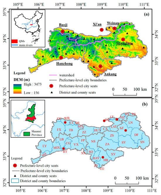
Figure 1.
Overview of the Qinling Mountains: (a) geographical range, elevation, district and county seats, and prefecture-level city seats in the QMs; (b) administrative division of prefecture-level cities and districts and counties in the QMs.
Notes: In the QMs, Xi’an has six districts and counties: Baqiao District (BQ), Lintong District (LT), Chang’an District (CA), Huyi District (HUY), Zhouzhi County (ZZ), and Lantian County (LAT); Baoji has six districts and counties: Weibin District (WB), Chencang District (CC), Qishan County (QS), Meixian County (MX), Taibai County (TB), and Fengxian County (FX); Weinan has four districts and counties: Linwei District (LW), Huazhou District (HZ), Huayin City (HY), and Tongguan County (TG); Hanzhong has nine districts and counties: Hantai District (HT), Chenggu County (CG), Yangxian County (YX), Xixiang County (XX), Mianxian County (MIX), Ningqiang County (NQ), Lueyang County (LY), Liuba County (LB), and Foping County (FP); Ankang City has seven districts and counties: Hanbin District (HB), Hanyin County (HAY), Shiquan County (SQ), Ningshan County (NS), Ziyang County (ZY), Langao County (LG), and Xunyang County (XY); Shangluo City has seven districts and counties: Shangzhou District (SZ), Luonan County (LN), Danfeng County (DF), Shangnan County (SN), Shanyang County (SY), Zhen’an County (ZA), and Zhashui County (ZS).
The QMs have a broad sense and a narrow sense; the narrow sense of the QMs mainly refers to the Qinling Mountains in Shaanxi Province, which is the core area of the Qinling Mountains embracing 12 national nature reserves [38]. The QMs (105°29′18″–111°01′54″ E, 32°28′53″–34°32′33″ N) cover an area of 58,800 km2, accounting for 28.59% of the total area of Shaanxi Province. From north to south, this province can be divided into the Loess Plateau of Northern Shaanxi Province, the Guanzhong basin zone, and the QMs [38,39]. The Guanzhong basin zone is at the heart of economic and cultural development, which is clustered by the provincial capital city Xi’an and its significant neighbor cities. The QMs is closely adjacent to the Guanzhong basin zone, spreading to the southernmost part of Shaanxi Province.
The QMs are divided into a south slope and a north slope by the watershed [36] and contain six prefecture-level cities, namely Xi’an, Weinan, Baoji, Hanzhong, Ankang, and Shangluo, and 39 districts and counties [40]. Baqiao District of Xi’an and Langao County of Ankang have relatively small land areas, neither exceeding 30 km2, while other districts and counties in the region have larger land areas, all exceeding 100 km2. Geographically, Weinan and Xi’an are located in the north slope, Hanzhong, Ankang and Shangluo are located in the south, while the districts and counties of Baoji are distributed on both north and south sides around the watershed.
Due to the tough mountainous conditions, inconvenient traffic, and insufficient cultivated land, social and economic development here is relatively backward. Especially, the QMs are on the list of the 14 centralized contiguously poor areas in China. In addition, in recent years, China has attached increasing importance to the ecological environmental protection of the QMs, and prohibits destruction of the natural environment. The urbanization and industrial development processes here are restricted, and higher requirements are put forward for the high-quality development of the local social economy. Therefore, the social economic development in the north slope of the QMs is relatively fast, while the social economic development in the south slope is relatively slow.
2.2. Research Framework
The research specifically includes the following three processes (Figure 2).
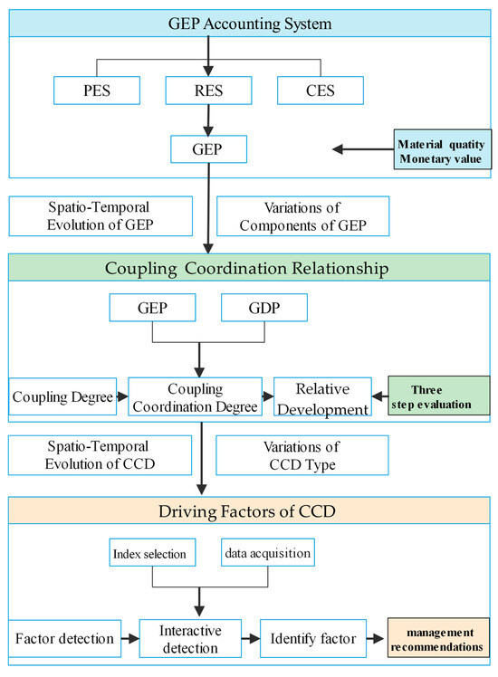
Figure 2.
Research framework for the study.
Firstly, ES types were first divided into three ES categories, Provisioning ecosystem services, Regulating ecosystem services, and Cultural ecosystem services, and the main ecosystem types in the QMs were selected. Within the framework of GEP accounting, remote sensing data, meteorological observation data, social economic data, and quantitative models such as RULSE and raster calculation methods were used to quantitatively evaluate the material quality of the ESs. Then, the monetary value of each ESs was quantitatively assessed through market value and other methods, so as to obtain the value of different ecosystem types and the total GEP value in the QMs.
Secondly, within the framework of the Coupling Coordination Degree, the three methods of Coupling Degree, Coupling Coordination Degree, and Relative Development Degree were comprehensively adopted to evaluate the interaction between GEP and GDP.
Thirdly, the geographic detector model was introduced, the driving factors of the relationship between GEP and GDP were selected, and the two methods of factor detection and interactive factor detection were used to quantitatively evaluate the contribution degree of different factors to the spatial differentiation of the relationship between GEP and GDP, and the main influencing factors that affect the development relationship were identified. In light of the need to maintain a balance between ecological environment and social economic development of nature reserves, corresponding countermeasures for sustainable development has been proposed.
Notes: GEP represents Gross Ecosystem Product, PES represents Provisioning ecosystem services, RES represents Regulating ecosystem services, CES represents Cultural ecosystem services, CD represents Coupling Degree, and CCD represents Coupling Coordination Degree.
2.3. Data Sources
We collect historical period data from multiple sources to carry out GEP accounting in the QMs. Specifically, the following types of data are introduced in Table 1:

Table 1.
Data source information.
- (1)
- Daily climate data of national meteorological stations in the QMs were downloaded from the China Meteorological Data Service Centre, and the meteorological elements included precipitation, temperature, etc. Then, with the meteorological elements, the local runoff and evaporation data were obtained using the hydrological formula;
- (2)
- Environmental data included air quality and water environment quality data, collected from Shaanxi Province air quality monitoring station and Shaanxi Provincial Department of Ecology and Environment, respectively;
- (3)
- Remote sensing data mainly included land use, soil, DEM, NPP, and NDVI. Since there were many types of remote sensing data involved, and the spatial resolutions of different data were significantly different, the remote sensing data were resampled to a resolution of 1000 m in the data processing process, and the data output resolution of ES and GEP assessment results were also set to 1000 m;
- (4)
- Social economic data, including GDP, population, water price, agricultural product price, tourist income, etc., were obtained from Shaanxi provincial statistical yearbook, Shaanxi provincial tourism development statistical bulletin, Shaanxi water conservancy statistical yearbook, etc. The statistical scale of social economic data is district-county scale, so the data output resolution of ES value evaluation results is also unified to district-county scale. Therefore, the total GEP results are also read with the same scale. In view of the fact that some districts and counties are not fully included in the scope of the QMs [40], the social economic statistics of these districts and counties are assigned within the coverage area by an area-weighted method.
2.4. Methods
2.4.1. GEP Accounting Methodology
This paper is based on the first provincial GEP accounting standard in China [42], where methods and models are chosen to calculate the quality and value of most ES types. Additionally, some popular models from previous studies are employed to assess remaining ESs, thereby establishing a more comprehensive GEP accounting framework in the QMs (Table 2) [20,27,33,43,44]. The specific models and algorithms employed in this study are detailed in the supplementary materials (Tables S1–S3).
Table 2.
Accounting scheme for Gross Ecosystem Product of the QMs.
First of all, the Millennium Ecosystem Assessment divides ESs into four ES categories: Provisioning ecosystem services (PES), Regulating ecosystem services (RES), Cultural ecosystem services (CES), and Supporting ecosystem services (SES) [12]. However, GEP accounts for the final goods and services provided by the ecosystem. Counting SES would result in double counting, leading to inflated results, so GEP only accounts for the final economic value of the first three ES categories [25,26,43]. Therefore, the types of ES are divided into PES, RES, and CES in the QMs (Table 2). Among them, PES includes five indicators such as agricultural products, RES includes eight indicators such as water conservation service, and CES is evaluated by ecological tourism service value.
Secondly, the biophysical value of the three types of ES is evaluated by the material quality method. Since most of these data are remote sensing data, the ES quality results are mainly raster data.
Thirdly, the monetary value of 14 indicators in three categories of ES with social economic data at district-county scale is evaluated.
Finally, the GEP of all districts and counties in the QMs is obtained by summing up the monetary values of the three ES types using the following formula:
where GEP represents Gross Ecosystem Product in the QMs, represents the value of PES, represents the value of RES, represents the value of CES [29]. The value of each ecosystem service is estimated by monetary value, and the unit is billion of the Chinese currency (CNY).
In the process of calculation, the GEP value is determined by utilizing climate and environmental data, soil erosion factor, vegetation cover factor, and social economic statistics specific to the region. Ultimately, the obtained results are compared and validated against relevant findings from previous studies [33,45].
2.4.2. Coupling Coordination Degree (CCD) Model
As a physical concept, coupling coordination is a common method used to evaluate the degree of interaction between different systems [29,46], which is widely used in the fields of economic development, urbanization, land use, ecological environment, and ecosystem services, etc. In this paper, the Coupling Coordination Degree (CCD) Model is used to study the dynamic interaction between GEP and GDP.
- Data standardization processing
Before the CCD analysis, in order to eliminate the differences in the dimensions of the indicators for the later calculation and comparative analysis, it is necessary to use the extreme value standardization method to normalize the GEP and GDP data to ensure that the index values of the two data are within the range of [0, 1], which is shown as follows [46]:
where refers to the standardized value of GEP or GDP, refers to the original value of GEP or GDP, and refer to the maximum and minimum of the original value of GEP or GDP, respectively.
- 2.
- Coupling Degree (CD) model
Coupling Degree refers to the relationship between two or more systems that interact and influence each other [46,47]. Therefore, we calculate the Coupling Degree of GEP and GDP for judging the relationship between the two systems:
where and refer to normalized data of GEP and GDP, respectively, refers to the coupling degree between GEP and GDP, with a value range of [0, 1]. An increasing value of C indicates a benign relationship between the two systems, and suggests that the development of the two systems tends to follow an orderly pattern; a decreasing value of C indicates a weaker coupling state between the two systems, and the two systems tend to develop in a disordered manner [48]. According to previous research, this paper divides the coupling degree of the two systems into four states ranging from high to low based on the C value [49]: low-level coupling (LC, 0 < C ≤ 0.3), antagonistic development (AD, 0.3 < C ≤ 0.6), running-in development (RD, 0.5 < C ≤ 0.8), and high-level coupling (HLC, 0.8 < C ≤ 1).
- 3.
- Coupling Coordination Degree (CCD) model
Coupling Degree can effectively characterize the interaction between multiple systems; however, it solely represents a resonance relationship, which fails to adequately reflect the overall synergy effect and development level between multiple systems [46]. On the basis of Coupling Degree, the Coupling Coordination Degree can provide a deeper reflection of the development of two systems [47]. The calculation formula is as follows:
where represents the comprehensive coordination index of these two subsystems, with a value range of [0, 1], and represent the contribution rates of the GEP and GDP subsystems in the eco-economic composite system, respectively, that is, the relative importance of them in the eco-economic system. Social economic development is as important as the ecological environment for a region, so both values are set at 0.5.
refers to the coupling coordination degree between GEP and GDP, with a value range of [0, 1], which can be obtained by combining the coupling degree and comprehensive coordination index. A high value of D indicates that GEP and GDP are mutually promoting at a high level in the eco-economic system, while a low value of indicates that they are mutually restricting in the overall system. According to previous studies [29] and the local social development, the coupling coordination degree between GEP and GDP is divided into five levels from high to low (Table 3): severe unbalance (SU, 0 < D ≤ 0.2), moderate unbalance (MU, 0.2 < D ≤ 0.4), slight coordination (SC, 0.4 < D ≤ 0.6), moderate coordination (MC, 0.6 < D ≤ 0.8), and high coordination (HC, 0.8 < D ≤ 1).
Table 3.
Coupling coordination levels and types of GEP and GDP.
- 4.
- Relative Development Degree (RDD) model
Though CCD can better reflect the mutual relationship between GEP and GDP in the eco-economic system, however, there is no consideration of the development rate or the development gap between them [39]. Therefore, on the basis of Coupling Coordination Degree results, it is necessary to introduce Relative Development Degree, which calculates the ratio of normalized GEP to GDP, in order to continue measuring relative development status between GEP and GDP in the eco-economic system. It is easy to know whether the regional development status of the ecosystem is ahead of or behind the development of the economy relatively with the following calculation formula:
where and refer to normalized GEP and GDP, respectively, represents the relative development status of these two subsystems in the eco-economic system. Based on the relevant research results and the quotient of normalized GEP and GDP, the RDD in the QMs is divided into three types: GEP lag, GDP lag, and Balance [29,39]. Among them, GEP lag indicates that ecology lags behind economic development, GDP lag indicates that the economy lags behind the ecological status, and Balance indicates that ecology and the economy have achieved synchronous and balanced development.
Finally, combined with CD, CCD, and RDD, this paper constructs a comprehensive coupling coordination analysis framework between GEP and GDP in the QMs (Table 3).
2.4.3. Geographic Detector Model
The geographic detector model can better detect the spatial heterogeneity of geographical phenomena, effectively explore the contribution of different driving factors to geographical differentiation, and analyze the impact of interaction between variables on the driving process, which has become an important tool for driving analysis in spatial statistics [50].
- Factor detection
In this study, the contribution of each single factor (X) to the spatial variation of dependent variable CCD (Y) was investigated by using the factor detection method. The calculation method is as follows:
where represents the contribution degree of a factor (X) to the spatial variation of CCD (Y), represents the stratification or partitioning of Y or X, and represent the sample size of the whole region and the sample size of layer h, and represent the variance of the whole region and the intra-layer variance of layer h, respectively. The value of is between 0 and 1, and the larger the value of , the higher the contribution of the factor to spatial variation.
- 2.
- Interaction detector
Interactive detection can detect the interpretation degree of the spatial variation of CCD when two factors (X1 and X2) act simultaneously.
Firstly, the q values of X1 and X2 contributing to the change of Y, namely q(X1) and q(X2), are calculated, and then the interaction q value (q(X1∩X2)) is calculated. The interaction relationship between the two factors is determined by judging the value of q(X1), q(X2), and q(X1∩X2). For the specific calculation principle and process, refer to the literature [50].
On this basis, the interaction of the two factors can be divided into five types: nonlinear weakening, single-factor nonlinear weakening, two-factor enhancement, independent, and nonlinear enhancement. When q(X1∩X2) > max (q(X1), q(X2)), the relationship between X1 and X2 is two-factor enhanced; when q(X1∩X2) > q(X1) + q(X2), the relationship is nonlinear enhanced [50].
- 3.
- The selection and processing of indicators
The spatial differentiation of regional CCD is influenced by natural environment conditions and local social economic development. Therefore, CCD is taken as the explained variable (Y) of this study. Based on the natural environment characteristics, regional development status of the QMs, and relevant studies [51,52], we select temperature (TEM, X1), precipitation (PRE, X2), altitude (X3), slope (X4), NDVI (X5) as key natural environmental factors, Aggregation index (AGI, X6), Landscape shape index (LSI, X7), Shannon diversity index (SDI, X8), Shannon evenness index (SEI, X9), Contagion index (CAI, X10) as Landscape pattern indices, and density of road network (RND, X11), and density of population (POD, X12) as factors which reflect social economic development (Table 4).
Table 4.
Driving factors for the CCD between GEP and GDP.
In data processing, the vector layers of six landscape pattern indices from 2010 to 2020 were calculated using the moving window method in Fragstats 4.2, based on the land use data. At the same time, since geographic detectors are effective at processing type variables, this study first processed variables X1–X12 as categorical variables using the natural split point method in the ArcGIS 10.6 platform. Then, according to the boundaries of different districts and counties, the type variables of different indicators in different regions are obtained using the tool Zonal Statistics as Table in the ArcGIS platform, so that the driving force analysis can be carried out with the geographic detector.
3. Results
3.1. Spatial Variations of ESs and GEP
3.1.1. Variations of PES from 2010–2020
From 2010 to 2020, PES in the QMs had obvious spatio-temporal changes (Figure 3). In 2010, PES took on a spatial pattern of high in the east and low in the west. The lowest PES values were scattered in Langao County, Tongguan County, Baqiao District, and Foping County, with PES lower than 0.01 billion CNY, while the highest PES values were distributed in Zhouzhi County and Weibin District, with PES higher than 2.00 billion CNY. In 2015, the PES of most districts and counties showed a certain increasing tendency, and only Weibin District, Linwei District, and Lintong District had a certain decrease in PES. In 2020, the increase rate of PES in various districts and counties was growing faster; only the PES of Chang’an decreased, while the increasing amount of Weibin exceeded 4 billion CNY. A total of eight districts and counties in the region exceeded 2.00 billion CNY.
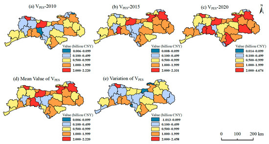
Figure 3.
Spatial distribution of the monetary value of PES in the QMs from 2010 to 2020.
In the whole QMs, the cumulative PES values of all districts and counties in 2010, 2015, and 2020 were 29.28 billion, 35.86 billion, and 51.30 billion CNY, respectively. Over the years, PES in the whole area showed a continuous upward tendency, with a growth rate of 75.17%. In terms of stage change, the growth rate of PES in the first five years was 22.44%, while the greater growth rate in the second five years reached 43.06%.
3.1.2. Variations of RES during 2010–2020
From 2010 to 2020, the spatial pattern of RES showed the distribution characteristics of high values in the east and west, and low values in the north and south (Figure 4). In 2010, the highest values were found in Ningshan County, Zhen’an County, and Shanyang County in the eastern and central QMs, with RES values exceeding 20 billion CNY. In 2015, a total of 28 districts and counties saw a decrease in RES compared with that in 2010, among which the reduction in RES of Shangzhou District and Shanyang County was more than 2.0 billion CNY. In 2020, RES in the whole region had a relatively obvious downward tendency, and a total of 35 districts and counties had an increase in RES compared with 2015, including six districts and counties with an increase of more than 2.0 billion CNY. From 2010 to 2020, a total of 15 districts and counties in the region showed a downward trend in RES, and almost all these districts and counties were distributed in the eastern region. Therefore, it was seen that although the RES value in the eastern region was larger, the downward trend was also more obvious.
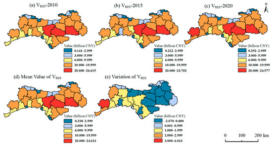
Figure 4.
Spatial distribution of the monetary value of RES in the QMs from 2010 to 2020.
In the whole region, the cumulative RES values of all districts and counties in 2010, 2015, and 2020 were 373.22 billion, 355.60 billion, and 390.05 billion CNY, respectively. RES in the whole region of the QMs had a fluctuation trend with a growth rate of 4.5% in the decade. In terms of stage change, the first five years showed a downward trend with a decline rate of 4.7%, and the second five years showed an upward trend with a growth rate of 9.7%. However, from the perspective of the magnitude of change, the changes in each county and district in this decade were not large.
3.1.3. Variations of CES during 2010–2020
The spatial pattern of CES underwent significant changes from 2010 to 2020 (Figure 5). In 2010, CES was generally higher in the east and lower in the west. There were five districts and counties with a value less than 0.10 billion CNY and five districts and counties with a value more than 2.00 billion CNY. In 2015, CES in the whole region increased significantly, and only Luonan County and Hanyin County showed a slight decline in CES. In 2020, there was a downward trend in eight districts and counties and an obvious increase in other regions in CES. In particular, Linwei District exceeded 20.00 billion CNY. In terms of total volume, seven districts and counties in the region were above 5 billion CNY in CES, and only nine districts and counties were below 1 billion CNY.
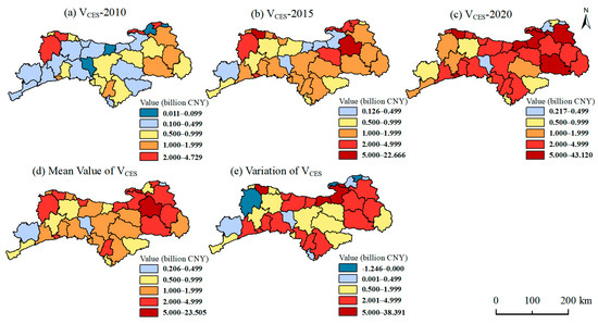
Figure 5.
Spatial distribution of the monetary value of CES in the QMs from 2010 to 2020.
For whole region, in 2010, 2015, and 2020, the cumulative CES values were 32.88 billion, 89.62 billion, and 148.24 billion CNY, respectively. The CES of the whole QMs showed a very obvious upward trend with the growth rate of 350.9% in the past decade. In terms of phase change, the growth rate of the first five years was 172.6%, and the growth rate of the second five years was 65.4%.
3.1.4. Variations of GEP during 2010–2020
From 2010 to 2020, the spatial pattern of GEP exhibited relatively similar spatial distribution characteristics to RES, namely high values in the east and west, and low values in the north and south (Figure 6). In 2010, the GEP values of all districts and counties were generally low, within the range from 0.45 to 29.46 billion CNY, and a total of 13 districts and counties had less than 6 billion CNY in GEP. The GEP values of Shangzhou District, Luonan County, Ningshan County, Zhen’an County, and Shanyang County were the highest, all exceeding 20 billion CNY. In 2015, only 11 districts and counties experienced a decrease in GEP, while the remaining districts and counties witnessed a significant increase in GEP. Notably, Linwei District’s GEP surpassed 10 billion CNY. In 2020, a decrease in GEP was observed in a total of five districts and counties, while the remaining areas exhibited a substantial increase in GEP. Specially, Linwei District witnessed an impressive surge of over 20 billion CNY in its GEP. A total of eight districts and counties had a GEP less than 6 billion CNY and two districts and counties achieved a GEP greater than 30 billion CNY. During 2010–2020, the average GEP of 12 districts and counties was lower than 6 billion CNY, while eight districts and counties had an average GEP of more than 20 billion CNY. The GEP of Huyi District and Lintong District exhibited a declining trend from 2010 to 2020, while Hanbin District, Lintong District, Lueyang County, Chang’an District, Weibin District, and Linwei District experienced prosperity with an increasing GEP. Particularly, the added value of GEP in Linwei District surpassed 40 billion CNY over the past decade.
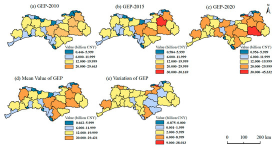
Figure 6.
Spatial distribution of GEP in the QMs from 2010 to 2020: (a–c) GEP Value, (d) mean value of GEP during 2010–2020, (e) variations of GEP during 2010–2020.
In 2010, 2015, and 2020, the cumulative GEP values of all districts and counties were 435.38 billion, 481.07 billion, and 589.58 billion CNY, respectively. In the past ten years, the GEP of the QMs showed a very continuous upward trend, with a growth rate of 35.4%. Meanwhile, the growth rate of the first five years was 10.5%, while the greater growth rate of the last five years reached to 22.6%.
The GEP of prefecture-level cities in the northern QMs was generally lower, while the GEP of prefecture-level cities in the southern QMs was generally higher (Figure 7). The list of cities ranked from lowest to highest in GEP were the following: Weinnan City, Xi’an City, Baoji City, Ankang City, Hanzhong City, and Shangluo City.

Figure 7.
Temporal variations of GEP in prefecture-level cities (a), ESs in the QMs (b), and in prefecture-level cities (c) from 2010–2020.
The economic value of RES constituted a significant proportion of the composition of GEP in the QMs. This was mainly because the QMs were key protection areas with well-protected ecological environments and high levels of biodiversity, allowing for effective utilization of ESs such as climate regulation. From 2010 to 2020, the proportion of RES in GEP in the QMs showed a continuous decreasing trend, while the proportion of PES and CES showed a continuous increasing trend. This was because in recent years the social economy, production activities, culture, and tourism industries in the QMs had developed, and the proportion of PES and CES in GEP increased significantly.
The GEP composition of these cities also reflected a relatively similar pattern of evolution. From 2010 to 2020, the proportion of CES in each city showed a continuous upward trend, and the proportion of RES showed a downward trend. The PES proportion in the southern QMs showed a certain increasing trend, while the proportion in the northern QMs showed an inter-annual fluctuation.
From a regional perspective, the proportion of CES in GEP is generally higher in the northern QMs. This can be attributed to their strategic location in the culturally rich and historically significant Guanzhong region, which boasts abundant cultural relics, scenic spots, and tourism resources that attract a relatively high level of tourism income. Among these regions, the contribution of CES to GEP in Weinnan City exceeded 60%.
3.2. Spatiotemporal Variations of the Coupling Relationship between GEP and GDP
3.2.1. Evolution Characteristics between CD and CCD
In 2010, the Coupling Degree (CD) between GEP and GDP was relatively low among districts and counties in the QMs, and the spatial distribution difference was significant (Figure 8). The districts and counties with a spatial coupling degree less than 0.6 (belonging to low-level coupling and antagonistic development states) accounted for 58.97%, mainly located in the central QMs. There were 18 districts and counties in antagonistic development state, and the CD values of Baqiao District and Langao County were the lowest. The districts and counties with high CD values accounted for 41.03%, mainly located in the northern and southern edge of QMs. The CD values reached the high-level coupling state in nine districts and counties, mainly distributed in the area to the north of the watershed, in which the Chang’an District and Weibin District had the highest CD values.

Figure 8.
Spatial distribution of CD and CCD between GEP and GDP in the QMs from 2010–2020.
In 2015, the coupling degree between GEP and GDP of the districts and counties was greatly improved. In space, the CD values of districts and counties were greater than 0.3, so there was no area of low-level coupling. The CD values of 10 districts and counties were in an antagonistic development state and these areas were mainly distributed in the western QMs. In the east, the CD values were generally higher, and the districts and counties with running-in development and high-level coupling state accounted for 16 and 13, respectively.
In 2020, the coupling degree between GEP and GDP improved significantly. The districts and counties with a high-level coupling state accounted for 84.62% of the whole region. During these years, there had been a significant improvement in the CD values across all regions, leading to an attainment of a relatively ideal state of the coupling relationship between GEP and GDP in 2020.
As for the Coupling Coordination Degree (CCD) between GEP and GDP in the QMs, this was relatively low in 2010, among which Baqiao District and Langao County had the lowest CCD values. There were 10 districts and counties in a severely unbalanced state, 28 districts and counties in a moderately unbalanced state, and only Shangzhou District in a slight coordination state.
In 2015, CCD in the QMs improved, and CCD in the eastern QMs improved significantly. The highest values of CCD were detected in Weibin District in the west and Shangzhou District in the east. In the central QMs, CCD was generally low in unbalanced development (severely unbalanced and moderately unbalanced state). The lowest CCD values of the whole region were distributed in Langao County and Baqiao District.
In 2020, CCD in the region increased significantly, and the scope of balanced development between GEP and GDP expanded. There were only 11 districts and counties with unbalanced CCD, which were mainly found in the northern and southern edge of the QMs. The CCD level in the eastern QMs was generally high, with six districts and counties’ CCD reaching a high coordination level. The CCD level in the central and western QMs was also relatively high. The highest values of CCD were seen in Hanbin District in the west and Weibin District in the east. Therefore, over these years, the CCD between GEP and GDP of all districts and counties showed a continuous upward trend, and the number of districts and counties reaching the coupling coordination state continued to increase. In 2020, most of the counties and counties in the QMs obtained a good coupling and coordination between GEP and GDP.
3.2.2. Evolution Characteristics of RDD and CDD Type
According to the relative development degree (RDD) of GEP and GDP, in 2010, the GDP of almost all districts and counties lagged behind the development of GEP (Figure 9). Only Weibin District, Baqiao District and Chang’an District were GEP lag areas. In 2015, the regional economy had a certain development in comparison with the ecological background, and there was a district, Huyi District, where the GEP and GDP reached a balanced development state. At the same time, Hantai District and Huayin City changed into GEP lag regions. In 2020, the spatial difference of the relative development of regional GEP and GDP was more obvious. In the eastern QMs, Lintong District, Shangzhou District, Luonan County, and Xunyang County developed into GEP–GDP balanced regions. The distribution range of the GEP lag area was remarkably large, with a total of 19 districts and counties mainly distributed in the northern fringe and the southeastern QMs. There were 16 districts and counties with GDP lag, mainly distributed in the central QMs.
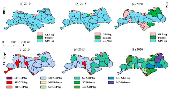
Figure 9.
Spatial distribution of RDD and CCD between GEP and GDP in the QMs from 2010–2020.
Based on relative development degree, combined with the corresponding CCD development status of each district and county, different development types were distinguished, and the coupling coordination relationship between GEP and GDP of each district and county was further analyzed. It could be seen that there were 11 types of coupling coordination relationship between GEP and GDP in all districts and counties of the QMs from 2010 to 2020.
Specifically, in 2010, only the interaction between GEP and GDP in Shangzhou District achieved slight coordination, so this region was in the state of GDP lag and coupling coordination development. MU–GDP lag regions were widely distributed in the QMs, accounting for 26 in total, which indicated that most regions of the QMs were in moderate unbalance and GDP lagged state. The regional distribution of SU-GDP lag exhibited a relatively large scale, accounting for nine districts and counties, mainly distributed in the western QMs.
In 2015, the relative development degree and CCD between GEP and GDP of several districts and counties changed greatly, which led to certain changes in the CDD types of 15 districts and counties in the QMs. Spatially, the distribution of MU–GDP lag was still relatively wide, but the total number reduced to 19. At the same time, three districts and counties changed from SU–GDP lag to MU–GDP lag, two districts and counties changed from MU–GDP lag to SC–GDP lag, and seven districts and counties changed from MU–GDP lag to SU–GDP lag. It indicated that, although the relative development degree of GEP and GDP in these regions did not change, the CDD type did change due to the change of CDD level.
In 2020, there were more CDD type changes in the whole region, reaching 33, and unchanged types were only found in six districts and counties. In total, two districts and counties changed from MU–GEP lag to SC–GEP lag, nine districts and counties changed from MU–GDP lag to SC–GDP lag, two districts and counties changed from SC–GEP lag to MC–GEP lag, and two districts and counties changed from SC–GDP lag to MC–GDP lag. Spatially, a total of four districts and counties reached simultaneous coupling coordination and balance, all of which were distributed in the eastern region, namely Luonan County, Shangzhou District, Lintong District, and Xunyang County. It showed that the development of the social economy and the protection of ecological environment in these regions was coordinated well and maintained in a good balance.
3.3. Driving Factors Affecting the Coupling Coordination Degree between GEP and GDP
3.3.1. Factor Detection Analysis
From 2010 to 2020, there were significant differences in various driving factors influencing the CCD between GEP and GDP in the whole region (Figure 10). In 2010, the change of CCD was mainly influenced by elevation with the explanatory power q value surpassing 0.5. The other driving factors, such as PRE, CAI, TEM, and POD, exceeded 0.3 at a moderate intensity, indicating that these factors also had a great influence on the change of CCD. In 2015, the change of CCD was mainly influenced by elevation and TEM, both of which had q values above 0.4, but not above 0.5. At the same time, it also reflected that the influence of TEM on CCD had been enhanced, while the influence of elevation had a certain downward trend. In addition, CAI, PRE, NDVI, SEI, and other factors had great influence on CCD, and their q values were all higher than 0.3. It can be seen that the influence of PRE and ROD on CCD waned, while the influence of NDVI on CCD significantly enhanced. In 2020, CAI had significantly enhanced its influence on CCD (q > 0.4) and became the main driving factor of regional CCD change; SDI’s q value also increased greatly, and it became the driving factor of CCD change along with TEM, elevation, POD, and NDVI (q > 0.4), while the influence of PRE on CCD decreased (q < 0.2).
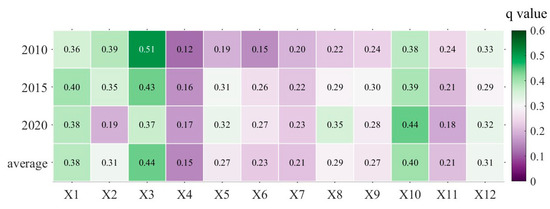
Figure 10.
Contribution rates of driving factors of CCD between GEP and GDP from 2000 to 2020.
From the perspective of multi-year average state, q values of elevation (X3), CAI (X10), TEM (X1), POD (X12), and PRE (X2) were relatively large, which indicated that natural factors and social economic development had a great impact on the coupling interaction between GEP and GDP in the QMs. However, LSI (X7), ROD (X11), slope (X3), and other factors had limited influence on the coupling relationship between GEP and GDP. In addition, the influence of different factors on CCD had a large inter-year fluctuation, which also indicated that CCD was more sensitive to changes in the social economy and natural environment.
3.3.2. Interaction Detection Analysis
By employing interaction detection, the impact of driving factors on the spatial differentiation of CCD in different years can be further investigated. These years, under the pairwise interaction of influencing factors, the contribution degree q to the spatial variation of CCD was greatly enhanced (Figure 11). These results indicated that these factors had a good synergistic effect on the spatial variation of CCD in the QMs and could promote or inhibit the spatial variation of CCD at the same time. From the perspective of the category, these interaction types were mainly manifested as nonlinear enhancement, and a small number of factors were manifested as bifactorial enhancement.
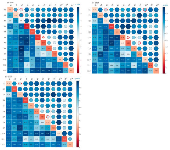
Figure 11.
Interaction detection results of driving factors of CCD between GEP and GDP from 2000 to 2020. Hexagons with red dashed edges represent the interaction type as bivariate enhancement, while the rest indicate the interaction type as nonlinear enhancement.
In 2010, the interaction between elevation and SDI was strong, and the strongest interaction occurred between elevation and SDI (q = 0.995). In addition, the interactions between TEM and SEI, and slope and SEI were also strong (q > 0.9). On the whole, ROD had the most significant influence in the interactions. The q values of its interactions with seven factors exceeded 0.9.
In 2015, the interaction of the two factors was relatively weaker than that of 2010. A total of eight groups of factors had a significant interactive impact (q > 0.9). The strongest interaction was between slope and LSI (q = 0.938). In addition, three groups had an interaction effect value of more than 0.9 with POD, indicating that population density still played a key role in the change of CCD at this stage, and had a greater impact on the change of CCD through the interactions with other indicators.
In 2020, there were still eight groups of factors with a significant interactive impact (q > 0.9), and four groups of CAI and other factors had a significant interactive impact (q > 0.9). The strongest interaction was between CAI and SDI (q = 0.977). In addition, over the course of three years, the interaction effect of population density on CCD showed a consistent decreasing trend.
4. Discussion
4.1. Implications of GEP Assessment
The comprehensive evaluation of regional ecosystem function and the integrated accounting of ecosystem value are multifaceted processes [19,26,53]. In the previous calculation process, the quality assessment makes accurate calculations of different ESs on the basis of different localized parameters and models, which required a large workload. However, the types of ESs vary widely, so it was difficult to directly sum up the total value of ESs. In contrast, the value assessment sets the ESs proper value coefficients, so as to estimate their value at each unit area simply and intuitively [24,54]. However, ignoring the heterogeneity of ecosystems in different spatial ranges would bring about difficulties in characterizing the dynamic change process of ecosystem quality, which would obstruct the application of this method.
GEP accounting integrates the advantages of the two methods and overcomes these research gaps well. First, the biological mechanism model in GEP accounting can comprehensively evaluate the quantity of ESs, taking of the heterogeneity of ESs fully into consideration. Subsequently, GEP adopts the market value method to further calculate the economic value of each ES and the total value of the regional ecosystem.
From 2010 to 2020, GEP in the QMs showed a trend of continuous growth, which was mutually confirmed with the continuous construction of ecological projects and the continuous improvement of ecological environment quality in the QMs. The north slope was close to the urban agglomeration of Guanzhong Plain, and the ecosystem was greatly disturbed by urbanization, so the GEP was relatively small. The southern slope was the core area of the QMs with better ecological environment quality. As for GEP composition, RES played a leading role. The stability and health of the ecosystem in the southern QMs ensured the continuous operation of RES and maintained the stable development of the local GEP. Secondly, the proportion of RES in GEP had consistently decreased from 2010 to 2020, while the proportion of PES and CES continued to rise, which indicated that the social economy of the QMs had achieved significant development. The relationship between the social economy and GEP, as well as the impact of social economic development on the ecological environment, deserves more attention in the QMs.
Over the years, the concepts of natural capital, ecological assets, ESs, GEP, and the contribution of nature to human beings have been put forward successively, and the supporting role of the ecosystem to human social economic development has been analyzed deeply. GEP accounting effectively integrates physical quantity and ecological asset value, and can systematically evaluate the overall benefits of the ecosystem to human society. The framework can carry out value accounting for forest, grassland, desert, and urban ecosystems, and can integrate detailed accounting indicators and localized parameters on the basis of more accurate ecosystem assessment at the national or regional level. Therefore, it can be widely used in the assessment of the overall status of the regional ecosystem and ecological protection effectiveness, the accounting of ecological assets, the implementation of inter-regional ecological compensation, and the evaluation of social sustainable development.
4.2. Interaction between GEP and GDP
The relationship between the ecosystem and economic development is characterized by mutual constraints and reciprocal influences. Only by promoting the benign interaction and coupling coordination of ecology and the economy can we gradually realize the sustainable development of society. The preservation of a sound ecological environment and the provision of high-quality ecosystem services are the primary objectives for regional development in the QMs. However, this region is also a typical poverty-stricken area, so it is equally important to improve the life and well-being of local residents. Therefore, it is imperative to effectively harmonize social economic development with the ecosystem and appropriately foster social economy while ensuring the ecological environment’s quality and ecosystem health. This is pivotal for achieving sustainable and high-quality development in local society.
In this study, the coupling degree and the coupling coordination degree between GEP and GDP in the QMs showed a continuous improvement from 2010 to 2020. In terms of CD, most districts and counties were in a state of high-level coupling between GEP and GDP. In terms of CCD, similarly, in 2020, most districts and counties in the QMs showed slight and moderate coordination between GEP and GDP, but there was no highly coordinated development between GEP and GDP in the region. There was a significant difference between CD and CCD relationship in this region. It can be seen that, on the one hand, the two methods can fairly consistently represent the regions where GEP and GDP have a close relationship and develop in an orderly manner. On the other hand, CCD can further reflect the synergic development effect of the two subsystems as compared with CD. Therefore, CCD is a more accurate way to characterize the interaction between GEP and GDP.
Secondly, combined with the relative development degree, the development difference of GEP and GDP in the QMs can be further evaluated. Due to the ecological background and development orientation of nature reserves, most districts and counties exhibited a lag in GDP development compared to GEP. Therefore, in 2020, a certain number of districts and counties showed a balance between GEP and GDP, and many districts and counties showed the GEP lag development. Generally, due to the stability of the ecosystem structure of a region, GEP will remain in a relatively stable condition without the influence of external factors or human activities, and the situation of slow growth or stagnation may occur. At the same time, the growth rate of GDP may be significantly faster than that of GEP. Therefore, although GEP in the QMs showed a trend of continuous increase over the years, the GDP growth rate was more rapid, resulting in GEP lagging behind GDP development in many districts and counties. Combined with the relative development degree and CCD model, the coordinated development status and mutual relationship between GEP and GDP of various districts and counties in the QMs can be more clearly understood, providing a reference for the formulation of policies related to regional ecosystem management and social sustainable development.
From the single-factor-driven analysis process of CCD, both natural factors and social and economic development have great impacts on the CCD between GEP and GDP. In addition, the influence of different factors on CCD had a large inter-year fluctuation, which also indicates that CCD is more sensitive to changes in the social economy and natural environment. Elevation, CAI, temperature, population density, and precipitation are the main driving factors of CCD in the QMs. According to the interaction analysis, the influencing factors have a good nonlinear enhancement effect on the spatial variation of CCD. Among these years, elevation and SDI, slope and LSI, and CAI and SDI have the strongest interaction influences, which indicates that landscape ecological pattern interaction plays an important driving role in the spatial variation of CCD in the QMs. The POD had an obvious enhancement trend with other factors. Population density represents the impact of human activities on the natural environment and social economic conditions, so the population density plays a key role in the change of CCD. The alteration in population density will induce the modifications in other natural factors or social and human factors, thus intensifying their impacts on CCD. Therefore, in the process of sustainable development of the QMs, we need to pay more attention to the change of population density.
4.3. Policy Recommendations
The unique geographical location and mountain features have created diverse natural environment features and various ecosystems in the QMs. There are 12 national nature reserves and 21 provincial nature reserves in the QMs, so the QMs are important ecological barriers in central China and key national ecological functional areas. Therefore, in such nature reserves, the red line of ecological protection should be strictly observed according to the national main function zoning and regional ecological civilization construction. It would ensure that development, construction, and economic and industrial activities are not carried out within the red line, effectively protecting biodiversity, ecosystem stability and ecological environment quality. It would provide basic support for sustainable social development and ecological civilization construction in the region and surrounding areas.
Second, from the perspective of land use, the development of regional production and life activities will have certain encroachment or influence on regional ecological space [55,56,57,58]. However, in ecological functional areas, economic development and people’s well-being are also important contents of social development. Therefore, scientific and comprehensive research on the relationship between GEP and GDP in ecological functional areas should be carried out and reasonable economic development goals should be set to ensure that the economy operates within a controllable interval or threshold. There will be a good prospect through adjusting industrial structure, changing the mode of economic development, reducing the environmental impact of industrial development, and effectively promoting the balanced development of regional ecology and economy.
Thirdly, the ecological environment and ESs are both regional and external. As a nature reserve, apart from fulfilling the fundamental needs of local residents for ESs, it will also provide enhanced support for the maintenance of the ecological environment and social economic development of the surrounding region. Therefore, it is urgent to deepen the market value evaluation system of ecological products and ESs, and carry out an applicable GEP evaluation in the QMs. Only by fully understanding the real situation and evolutionary law of the local ecosystem, and quantitatively assessing the ecological relationship between different ESs types and the surrounding beneficiary areas in the QMs, can we determine the contribution degree of the ecosystem to local and regional socio-economic development and human welfare. On the basis of the ecological compensation system, economic compensation should be imposed for the loss of regions due to their inputs to protect ecosystems and the environment, and forgone opportunities for social economic development. Only in this way can we effectively ensure better coordination and sustainable development between regional ecology and economy for some ecological functional areas that are unable develop their economy on a large scale.
Fourth, the relationship between the ecosystem and the social economy is complicated. In the early stage of development, the rapid increase in GDP was obtained through the massive consumption of natural resources, which led to great destruction of the ecological environment, and there was a great contradiction between the two. After reaching a turning point in economic development, the regional industrial structure has undergone an upgrade, leading to advancements in environmental protection technology and scientific research. Consequently, the ecological environment quality has been enhanced by economic progress. In this study, after ten years of development, the coupling coordination relationship between GEP and GDP in most areas is in a benign state, which indicates that while the social economy of various districts and counties is developing rapidly, the ecological benefits and welfare provided by the ecosystem for the development of human society are also increasing steadily. However, from the perspective of relative development, until 2020, the development of GEP in many areas had lagged behind the development of the social economy. This shows that although the social economy and GEP in these places show synergistic growth, the growth rate of GEP is relatively slow, and the development of both has not yet attained an optimal equilibrium. Therefore, it is necessary to combine the coupling coordination degree with relative development degree to deeply study the relationship between GEP and GDP in different regions, delineate different types of the relationship between the two spatially, and conduct spatial management by classification. We should focus on the districts and counties whose GDP lags behind the development of the ecological environment. While pursuing economic growth, we should fully consider the possible impact of development on the ecosystem, rationally utilize natural resources, and gradually realize the harmonious development of ecology and economy.
4.4. Limitations and Future Research
In different regions, there are great differences in ES types. In the study of GEP in the QMs, typical and important ESs were selected for ecological value accounting according to regional characteristics. Some regulating services, such as pest control, wind prevention, and sand fixation, etc., were not taken into account. In addition, in the accounting of ecosystem cultural functions, most studies take the tourism resource value of natural landscape as representative. Therefore, in the current GEP accounting studies, due to the variations in the selection of ES types and inherent limitation of capturing all local ES types, the obtained results will be smaller than the true GEP value.
In addition, the selected model and specific parameters will also have an impact on the calculation results. First of all, for the same ES, the selection of different models and different parameters will inevitably have an impact on the final result. Second, the calculation of GEP involves not only quantitative data such as physical geography, but also a lot of social economy data. The latter type of data are often statistical data, which are difficult to characterize in a spatial raster, so there is a problem of scale mismatch between the GEP and raster data in model calculation. Therefore, the calculation results of some ES types can only be counted in districts and counties. This affects the accuracy of calculation results. Third, due to data limitations, it is difficult to make long-term time series or year-by-year ecosystem assessments.
Of course, as a relatively innovative assessment framework of ES value, GEP can comprehensively assess the ecological value of the final products and services provided by the ecosystem for human survival, and effectively incorporate environmental and ecological benefits into the evaluation of social economic development. It provides scientific reference for ecological asset assessment and ecological civilization construction. From the perspective of practice, although GEP accounting standards have been preliminarily established at the national, provincial, and regional levels, there are still differences in accounting standards and ES types, which need to be further deepened and improved. Meanwhile, due to the heterogeneity of geographical environment and regional differences of social economic factors, the applicability of different models and the localization of parameters in ES assessment still need to be strengthened. The accuracy and accessibility of data is a necessary condition for conducting research. If the grid processing of social economic data and the collection density of social statistics data can be improved, the accuracy of ES value assessment will be enhanced.
5. Conclusions
In this paper, the QMs region was taken as a remarkable example, and multi-source data including meteorological data, environmental data, remote sensing data, and social economic data were used to quantitatively assess the spatio-temporal evolution of ecosystem services and GEP, and the coupling coordination relationship between GEP and GDP.
The results show that: (1) From 2010 to 2020, the GEP in the whole QMs showed a continuous upward trend, and the spatial pattern of GEP exhibited the distribution characteristics of high values in the east and west, and low values in the north and south. (2) The GEP composition in the QMs included RES, PES, and CES, of which RES accounted for a relatively large proportion but has been declining in recent years. (3) The degree of coupling coordination between GEP and GDP of all districts and counties had shown a continuous upward trend, and the number of districts and counties reaching the state of coupling coordination continues to increase. By 2020, most of the counties and counties had achieved a satisfactory coupling coordination state between GEP and GDP. (4) The social economy of most districts and counties lagged behind GEP in 2010. However, this spatial pattern has been changing over time, with an increase in the number of districts and counties lagging in GEP in 2020. This indicates significant social economic development in the region. (5) Elevation, contagion, temperature, population density, and precipitation are the main driving factors influencing coupling coordination state between GEP and GDP. In the future, further research is needed to understand the relationship between the social economic development and GEP in these regions, such as nature reserves. Corresponding countermeasures should be taken to ensure the coordinated and sustainable development of the regional social economy and ecological environment.
Supplementary Materials
The following supporting information can be downloaded at: https://www.mdpi.com/article/10.3390/land13020234/s1, Table S1: Detailed accounting methods of Provisioning ecosystem service; Table S2: Detailed accounting methods of Regulating ecosystem service; Table S3: Detailed accounting methods of Cultural ecosystem service.
Author Contributions
Conceptualization, P.W. and K.L.; methodology, Y.C. and P.W.; software, Y.C. and P.W.; validation, Y.C., K.L. and P.W.; formal analysis, P.W. and Y.C.; investigation, Y.C., X.L. and L.Z.; resources, P.W., K.L. and L.C.; data curation, Y.C., P.W. and L.C.; writing—original draft preparation, P.W., Y.C. and L.C.; writing—review and editing, P.W., X.L., L.Z., L.C. and T.S.; visualization, P.L. and P.W.; supervision, G.Y., H.W., S.G. and J.Y.; project administration, J.Y. and K.L.; funding acquisition, K.L., P.W. and T.S. All authors have read and agreed to the published version of the manuscript.
Funding
This research was funded by the Natural Science Basic Research Program of Shaanxi Province of China (2021JQ-768), the Scientific Research Project of Shaanxi Provincial Education Department (21JK0306), National Natural Science Foundation of China (42001132), the Key Forestry Science and Technology Innovation Projects in Shaanxi Province (SXLK2023-02-4), the Social Science Foundation project of Shaanxi Province (2023H012), and the Social Science Planning Research Project of Shandong Province (22CGLJ40).
Data Availability Statement
All data and materials are available upon request.
Conflicts of Interest
The authors declare no conflicts of interest.
References
- Chaplin-Kramer, R.; Sharp, R.P.; Weil, C.; Bennett, E.M.; Pascual, U.; Arkema, K.K.; Brauman, K.A.; Bryant, B.P.; Guerry, A.D.; Haddad, N.M.; et al. Global modeling of nature’s contributions to people. Science 2019, 366, 255–258. [Google Scholar] [CrossRef]
- Díaz, S.; Pascual, U.; Stenseke, M.; Martín-López, B.; Watson, R.T.; Molnár, Z.; Hill, R.; Chan, K.M.A.; Baste, I.A.; Brauman, K.A.; et al. Assessing nature’s contributions to people. Science 2018, 359, 270–272. [Google Scholar] [CrossRef] [PubMed]
- Liu, Y.; Fu, B.; Wang, S.; Rhodes, J.R.; Li, Y.; Zhao, W.; Li, C.; Zhou, S.; Wang, C. Global assessment of nature’s contributions to people. Sci. Bull. 2023, 68, 424–435. [Google Scholar] [CrossRef] [PubMed]
- Pascual, U.; Balvanera, P.; Díaz, S.; Pataki, G.; Roth, E.; Stenseke, M.; Watson, R.T.; Başak Dessane, E.; Islar, M.; Kelemen, E.; et al. Valuing nature’s contributions to people: The IPBES approach. Curr. Opin. Environ. Sustain. 2017, 26–27, 7–16. [Google Scholar] [CrossRef]
- Peng, J.; Xia, P.; Liu, Y.; Xu, Z.; Zheng, H.; Lan, T.; Yu, S. Ecosystem services research: From golden era to next crossing. Trans. Earth Environ. Sustain. 2023, 1, 9–19. [Google Scholar] [CrossRef]
- Liu, Q.; Qiao, J.; Li, M.; Huang, M. Spatiotemporal heterogeneity of ecosystem service interactions and their drivers at different spatial scales in the Yellow River Basin. Sci. Total Environ. 2024, 908, 168486. [Google Scholar] [CrossRef]
- Costanza, R.; dArge, R.; deGroot, R.; Farber, S.; Grasso, M.; Hannon, B.; Limburg, K.; Naeem, S.; Oneill, R.V.; Paruelo, J.; et al. The value of the world’s ecosystem services and natural capital. Nature 1997, 387, 253–260. [Google Scholar] [CrossRef]
- Bullock, J.M.; Aronson, J.; Newton, A.C.; Pywell, R.F.; Rey-Benayas, J.M. Restoration of ecosystem services and biodiversity: Conflicts and opportunities. Trends Ecol. Evol. 2011, 26, 541–549. [Google Scholar] [CrossRef]
- Watson, L.; Straatsma, M.W.; Wanders, N.; Verstegen, J.A.; de Jong, S.M.; Karssenberg, D. Global ecosystem service values in climate class transitions. Environ. Res. Lett. 2020, 15, 024008. [Google Scholar] [CrossRef]
- Helseth, E.V.; Vedeld, P.; Vatn, A.; Gómez-Baggethun, E. Value asymmetries in Norwegian forest governance: The role of institutions and power dynamics. Ecol. Econ. 2023, 214, 107973. [Google Scholar] [CrossRef]
- Costanza, R.; de Groot, R.; Braat, L.; Kubiszewski, I.; Fioramonti, L.; Sutton, P.; Farber, S.; Grasso, M. Twenty years of ecosystem services: How far have we come and how far do we still need to go? Ecosyst. Serv. 2017, 28, 1–16. [Google Scholar] [CrossRef]
- Millennium Ecosystem Assessment. Ecosystems and Human Well-Being: Synthesis; Island Press: Washington, DC, USA, 2005. [Google Scholar]
- Daily, G.C. Nature’s Services: Societal Dependence on Natural Ecosystems; Island Press: Washington, DC, USA, 1997. [Google Scholar]
- Tan, P.Y.; Zhang, J.; Masoudi, M.; Alemu, J.B.; Edwards, P.J.; Gret-Regamey, A.; Richards, D.R.; Saunders, J.; Song, X.P.; Wong, L.W. A conceptual framework to untangle the concept of urban ecosystem services. Landsc. Urban Plan. 2020, 200, 103837. [Google Scholar] [CrossRef] [PubMed]
- Zhang, Z.; Liu, Y.; Wang, Y.; Liu, Y.; Zhang, Y.; Zhang, Y. What factors affect the synergy and tradeoff between ecosystem services, and how, from a geospatial perspective? J. Clean. Prod. 2020, 257, 120454. [Google Scholar] [CrossRef]
- Jones, L.; Norton, L.; Austin, Z.; Browne, A.L.; Donovan, D.; Emmett, B.A.; Grabowski, Z.J.; Howard, D.C.; Jones, J.P.G.; Kenter, J.O.; et al. Stocks and flows of natural and human-derived capital in ecosystem services. Land Use Policy 2016, 52, 151–162. [Google Scholar] [CrossRef]
- Jiang, W.; Lü, Y.; Liu, Y.; Gao, W. Ecosystem service value of the Qinghai-Tibet Plateau significantly increased during 25 years. Ecosyst. Serv. 2020, 44, 101146. [Google Scholar] [CrossRef]
- Daily, G.C.; Söderqvist, T.; Aniyar, S.; Arrow, K.; Dasgupta, P.; Ehrlich, P.R.; Folke, C.; Jansson, A.; Jansson, B.-O.; Kautsky, N.; et al. The Value of Nature and the Nature of Value. Science 2000, 289, 395–396. [Google Scholar] [CrossRef] [PubMed]
- de Groot, R.; Brander, L.; van der Ploeg, S.; Costanza, R.; Bernard, F.; Braat, L.; Christie, M.; Crossman, N.; Ghermandi, A.; Hein, L.; et al. Global estimates of the value of ecosystems and their services in monetary units. Ecosyst. Serv. 2012, 1, 50–61. [Google Scholar] [CrossRef]
- Ouyang, Z.; Zheng, H.; Xiao, Y.; Polasky, S.; Liu, J.; Xu, W.; Wang, Q.; Zhang, L.; Xiao, Y.; Rao, E.M.; et al. Improvements in ecosystem services from investments in natural capital. Science 2016, 352, 1455–1459. [Google Scholar] [CrossRef]
- Yu, Y.; Li, J.; Han, L.; Zhang, S. Research on ecological compensation based on the supply and demand of ecosystem services in the Qinling-Daba Mountains. Ecol. Indic. 2023, 154, 110687. [Google Scholar] [CrossRef]
- Wang, P.; Zhang, L.; Li, Y.; Jiao, L.; Wang, H.; Yan, J.; Lü, Y.; Fu, B. Spatio-temporal variations of the flood mitigation service of ecosystem under different climate scenarios in the Upper Reaches of Hanjiang River Basin, China. J. Geogr. Sci. 2018, 28, 1385–1398. [Google Scholar] [CrossRef]
- Sannigrahi, S.; Chakraborti, S.; Joshi, P.K.; Keesstra, S.; Sen, S.; Paul, S.K.; Kreuter, U.; Sutton, P.C.; Jha, S.; Dang, K.B. Ecosystem service value assessment of a natural reserve region for strengthening protection and conservation. J. Environ. Manag. 2019, 244, 208–227. [Google Scholar] [CrossRef] [PubMed]
- Xie, G.; Zhang, C.; Zhen, L.; Zhang, L. Dynamic changes in the value of China’s ecosystem services. Ecosyst. Serv. 2017, 26, 146–154. [Google Scholar] [CrossRef]
- Ouyang, Z.; Zhu, C.; Yang, G.; Xu, W.; Zheng, H.; Zhang, Y.; Xiao, Y. Gross ecosystem product: Concept, accounting framework and case study. Acta Ecol. Sin. 2013, 33, 6747–6761. [Google Scholar] [CrossRef]
- Ouyang, Z.; Song, C.; Zheng, H.; Polasky, S.; Xiao, Y.; Bateman, I.J.; Liu, J.; Ruckelshaus, M.; Shi, F.; Xiao, Y.; et al. Using gross ecosystem product (GEP) to value nature in decision making. Proc. Natl. Acad. Sci. USA 2020, 117, 14593–14601. [Google Scholar] [CrossRef] [PubMed]
- Zou, Z.; Wu, T.; Xiao, Y.; Song, C.; Wang, K.; Ouyang, Z. Valuing natural capital amidst rapid urbanization: Assessing the gross ecosystem product (GEP) of China’s ‘Chang-Zhu-Tan’ megacity. Environ. Res. Lett. 2020, 15, 124019. [Google Scholar] [CrossRef]
- Wang, W.; Xu, C.; Li, Y. Priority areas and benefits of ecosystem restoration in Beijing. Environ. Sci. Pollut. Res. Int. 2023, 30, 83600–83614. [Google Scholar] [CrossRef]
- Xie, H.; Li, Z.; Xu, Y. Study on the Coupling and Coordination Relationship between Gross Ecosystem Product (GEP) and Regional Economic System: A Case Study of Jiangxi Province. Land 2022, 11, 1540. [Google Scholar] [CrossRef]
- Zang, Z.; Zhang, Y.; Xi, X. Analysis of the Gross Ecosystem Product—Gross Domestic Product Synergistic States, Evolutionary Process, and Their Regional Contribution to the Chinese Mainland. Land 2022, 11, 732. [Google Scholar] [CrossRef]
- Ma, Q.; Zhou, M.; Liu, J.; Zhao, J.; Xi, M. Coupling Relationship between Ecosystem Service Value and Socioeconomic Development in the Qinba Mountains, China. Diversity 2022, 14, 1105. [Google Scholar] [CrossRef]
- Guan, S.; Liao, Q.; Wu, W.; Yi, C.; Gao, Y. Revealing the Coupling Relationship between the Gross Ecosystem Product and Economic Growth: A Case Study of Hubei Province. Sustainability 2022, 14, 7546. [Google Scholar] [CrossRef]
- Jiang, H.; Wu, W.; Wang, J.; Yang, W.; Gao, Y.; Duan, Y.; Ma, G.; Wu, C.; Shao, J. Mapping global value of terrestrial ecosystem services by countries. Ecosyst. Serv. 2021, 52, 101361. [Google Scholar] [CrossRef]
- Ge, Y.; Hu, S.; Ren, Z.; Jia, Y.; Wang, J.; Liu, M.; Zhang, D.; Zhao, W.; Luo, Y.; Fu, Y.; et al. Mapping annual land use changes in China’s poverty-stricken areas from 2013 to 2018. Remote Sens. Environ. 2019, 232, 111285. [Google Scholar] [CrossRef]
- Sun, X.; Lu, H.; Wang, S.; Xu, X.; Zeng, Q.; Lu, X.; Lu, C.; Zhang, W.; Zhang, X.; Dennell, R. Hominin distribution in glacial-interglacial environmental changes in the Qinling Mountains range, central China. Quat. Sci. Rev. 2018, 198, 37–55. [Google Scholar] [CrossRef]
- Qi, G.; Bai, H.; Zhao, T.; Meng, Q.; Zhang, S. Sensitivity and areal differentiation of vegetation responses to hydrothermal dynamics on the northern and southern slopes of the Qinling Mountains in Shaanxi province. J. Geogr. Sci. 2021, 31, 785–801. [Google Scholar] [CrossRef]
- Zhao, T.; Bai, H.; Yuan, Y.; Deng, C.; Qi, G.; Zhai, D. Spatio-temporal differentiation of climate warming (1959–2016) in the middle Qinling Mountains of China. J. Geogr. Sci. 2020, 30, 657–668. [Google Scholar] [CrossRef]
- Shang, X.; He, Z.; Chen, W.; He, L.; Yang, H. Changes and response mechanisms of leaf area index and evapotranspiration in the typical natural landscapes of the Loess Plateau in northern Shaanxi of China under the human intervention. Ecol. Indic. 2023, 154, 110517. [Google Scholar] [CrossRef]
- Zou, C.; Zhu, J.; Lou, K.; Yang, L. Coupling coordination and spatiotemporal heterogeneity between urbanization and ecological environment in Shaanxi Province, China. Ecol. Indic. 2022, 141, 109152. [Google Scholar] [CrossRef]
- Taibai County People’s Government. Notice of General Office of Shaanxi Provincial People’s Government on Issuing the Overall Plan for Ecological and Environmental Protection of Qinling Mountains. Available online: https://www.taibai.gov.cn/art/2021/2027/2013/art_7770_2821.html (accessed on 15 December 2021).
- Zhang, D.; Zhang, X.; Bai, X.; Peng, J. A Dataset of 1km Grid Road Network Density in China (2019). Available online: https://cstr.cn/31253.11.sciencedb.02938 (accessed on 12 October 2023).
- Zhejiang Provincial Market Supervision and Administration Bureau. Technical Specification for Accounting Gross Ecosystem Product (GEP)—Terrestrial Ecosystems. DB33/T 2274-2020. Available online: http://zjamr.zj.gov.cn/art/2020/9/29/art_1229047334_58814039.html (accessed on 12 October 2023).
- Ni, R.; Wang, F.; Yu, J. Spatiotemporal changes in sustainable development and its driving force in the Yangtze River Delta region, China. J. Clean. Prod. 2022, 379, 134751. [Google Scholar] [CrossRef]
- Wen, Y.; Sun, Q.; Yan, Y.; Xiao, M.; Song, W.; Yang, J. Impacts of the terrestrial ecosystem changes on the carbon fixation and oxygen release services in the Guangdong-Hong Kong-Macao Greater Bay Area. Acta Ecol. Sin. 2020, 40, 8482–8493. [Google Scholar]
- Ma, G.; Yu, F.; Wang, J.; Zhou, X.; Yuan, J.; Mou, X.; Zhou, Y.; Yang, W.; Peng, F. Measuring gross ecosystem product (GEP) of 2015 for terrestrial ecosystems in China. China Environ. Sci. 2017, 37, 1474–1482. [Google Scholar]
- Guo, X.; Fang, C.; Mu, X.; Chen, D. Coupling and coordination analysis of urbanization and ecosystem service value in Beijing-Tianjin-Hebei urban agglomeration. Ecol. Indic. 2022, 137, 108782. [Google Scholar] [CrossRef]
- Sun, Y.; Liu, S.; Dong, Y.; An, Y.; Shi, F.; Dong, S.; Liu, G. Spatio-temporal evolution scenarios and the coupling analysis of ecosystem services with land use change in China. Sci. Total Environ. 2019, 681, 211–225. [Google Scholar] [CrossRef] [PubMed]
- Ding, T.; Chen, J.; Fang, Z.; Chen, J. Assessment of coordinative relationship between comprehensive ecosystem service and urbanization: A case study of Yangtze River Delta urban Agglomerations, China. Ecol. Indic. 2021, 133, 108454. [Google Scholar] [CrossRef]
- Yang, Y.; Bao, W.; Liu, Y. Coupling coordination analysis of rural production-living-ecological space in the Beijing-Tianjin-Hebei region. Ecol. Indic. 2020, 117, 106512. [Google Scholar] [CrossRef]
- Zhang, Y.; He, Y.; Li, Y.; Jia, L. Spatiotemporal variation and driving forces of NDVI from 1982 to 2015 in the Qinba Mountains, China. Environ. Sci. Pollut. Res. Int. 2022, 29, 52277–52288. [Google Scholar] [CrossRef] [PubMed]
- Li, L.; Fan, Z.; Feng, W.; Yuxin, C.; Keyu, Q. Coupling coordination degree spatial analysis and driving factor between socio-economic and eco-environment in northern China. Ecol. Indic. 2022, 135, 108555. [Google Scholar] [CrossRef]
- Hu, Z.; Gong, J.; Li, J.; Li, R.; Zhang, Z.; Zhong, F.; Wen, C. Valuing the coordinated development of urbanization and ecosystem service value in border counties. J. Clean. Prod. 2023, 415, 137799. [Google Scholar] [CrossRef]
- Weiskopf, S.R.; Rubenstein, M.A.; Crozier, L.G.; Gaichas, S.; Griffis, R.; Halofsky, J.E.; Hyde, K.J.W.; Morelli, T.L.; Morisette, J.T.; Munoz, R.C.; et al. Climate change effects on biodiversity, ecosystems, ecosystem services, and natural resource management in the United States. Sci. Total Environ. 2020, 733, 137782. [Google Scholar] [CrossRef] [PubMed]
- Costanza, R.; de Groot, R.; Sutton, P.; van der Ploeg, S.; Anderson, S.J.; Kubiszewski, I.; Farber, S.; Turner, R.K. Changes in the global value of ecosystem services. Glob. Environ. Chang. 2014, 26, 152–158. [Google Scholar] [CrossRef]
- Li, W.; Cai, Z.; Jin, L. Spatiotemporal characteristics and influencing factors of the coupling coordinated development of production-living-ecology system in China. Ecol. Indic. 2022, 145, 109738. [Google Scholar] [CrossRef]
- Fu, J.; Bu, Z.; Jiang, D.; Lin, G.; Li, X. Sustainable land use diagnosis based on the perspective of production–living–ecological spaces in China. Land Use Policy 2022, 122, 106386. [Google Scholar] [CrossRef]
- Liu, X.; Wang, X.; Chen, K.; Li, D. Simulation and prediction of multi-scenario evolution of ecological space based on FLUS model: A case study of the Yangtze River Economic Belt, China. J. Geogr. Sci. 2023, 33, 373–391. [Google Scholar] [CrossRef]
- Wang, A.; Liao, X.; Tong, Z.; Du, W.; Zhang, J.; Liu, X.; Liu, M. Spatial-temporal dynamic evaluation of the ecosystem service value from the perspective of “production-living-ecological” spaces: A case study in Dongliao River Basin, China. J. Clean. Prod. 2022, 333, 130218. [Google Scholar] [CrossRef]
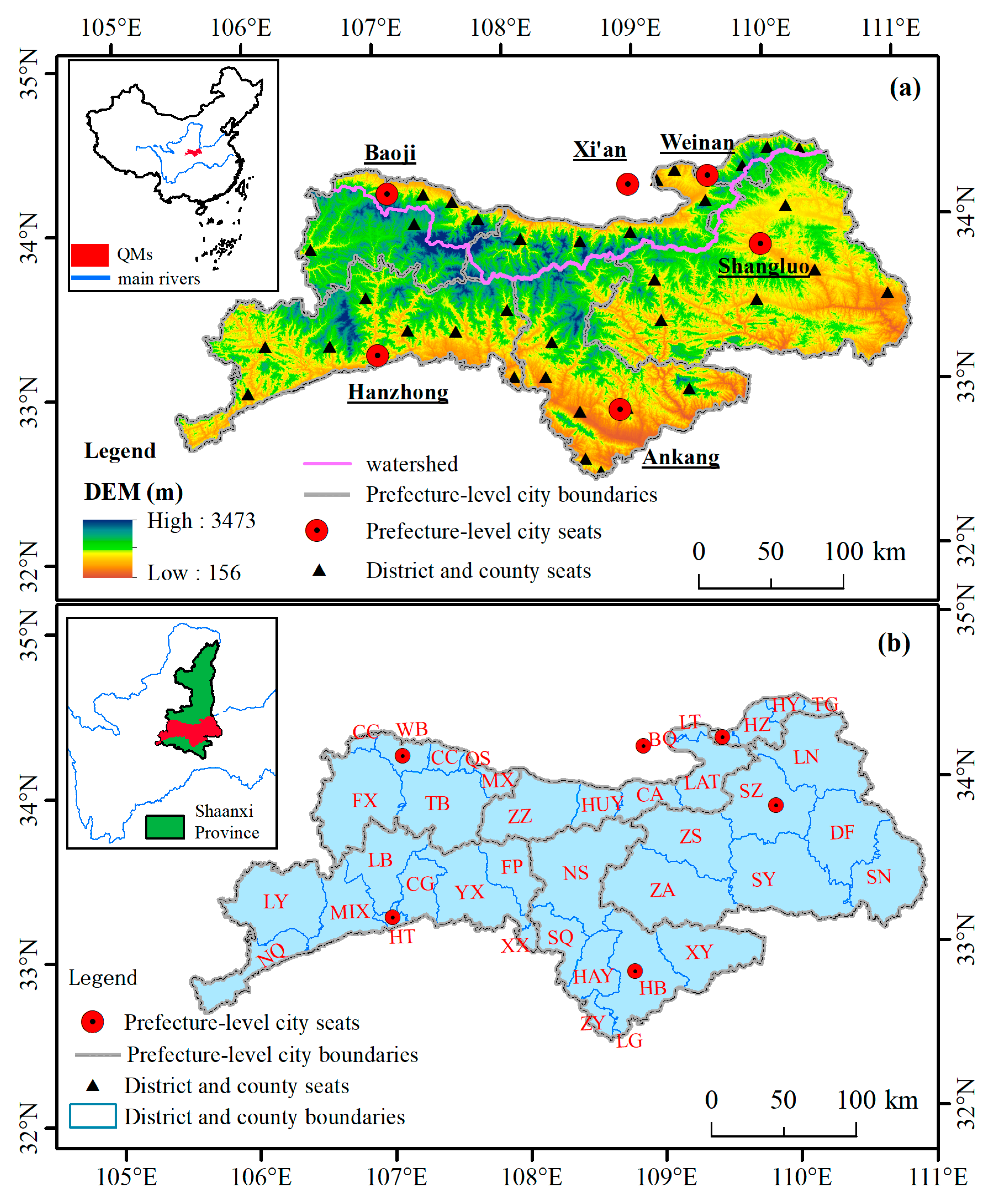
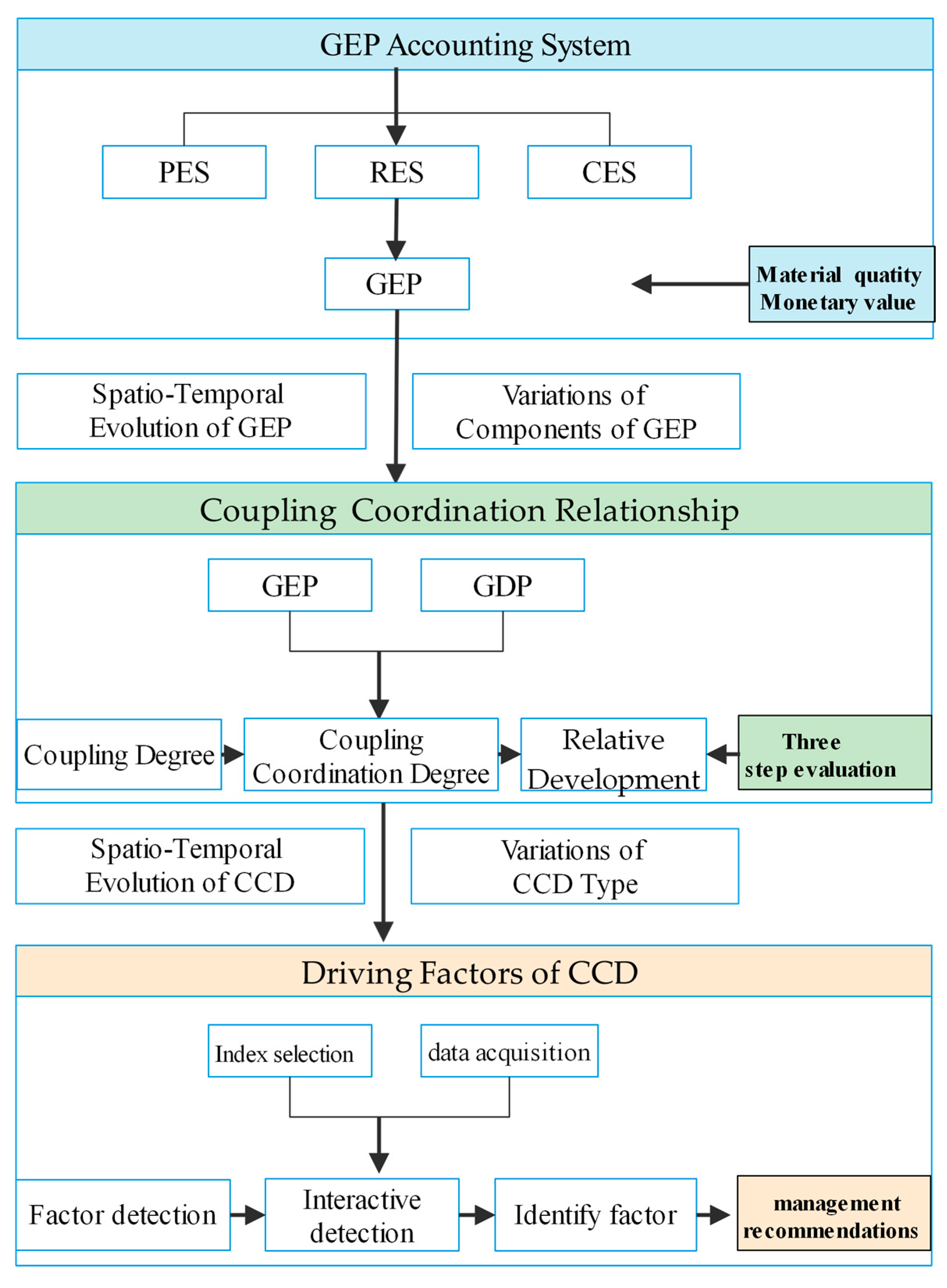
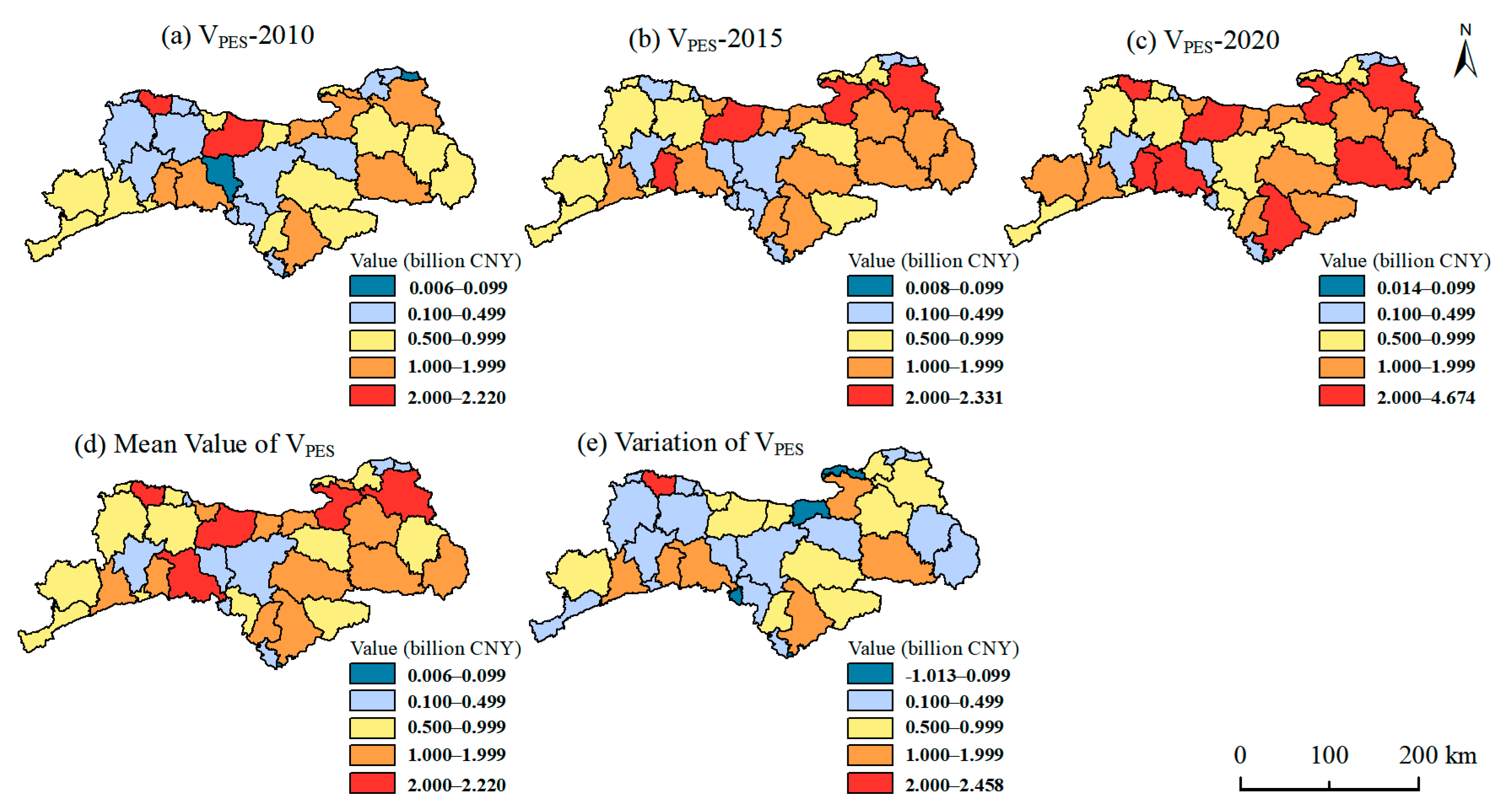
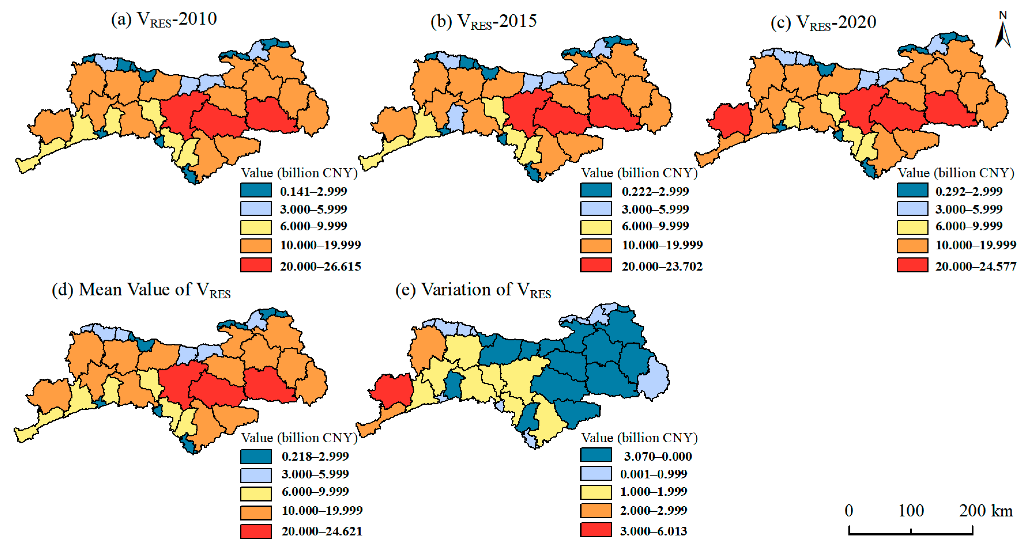
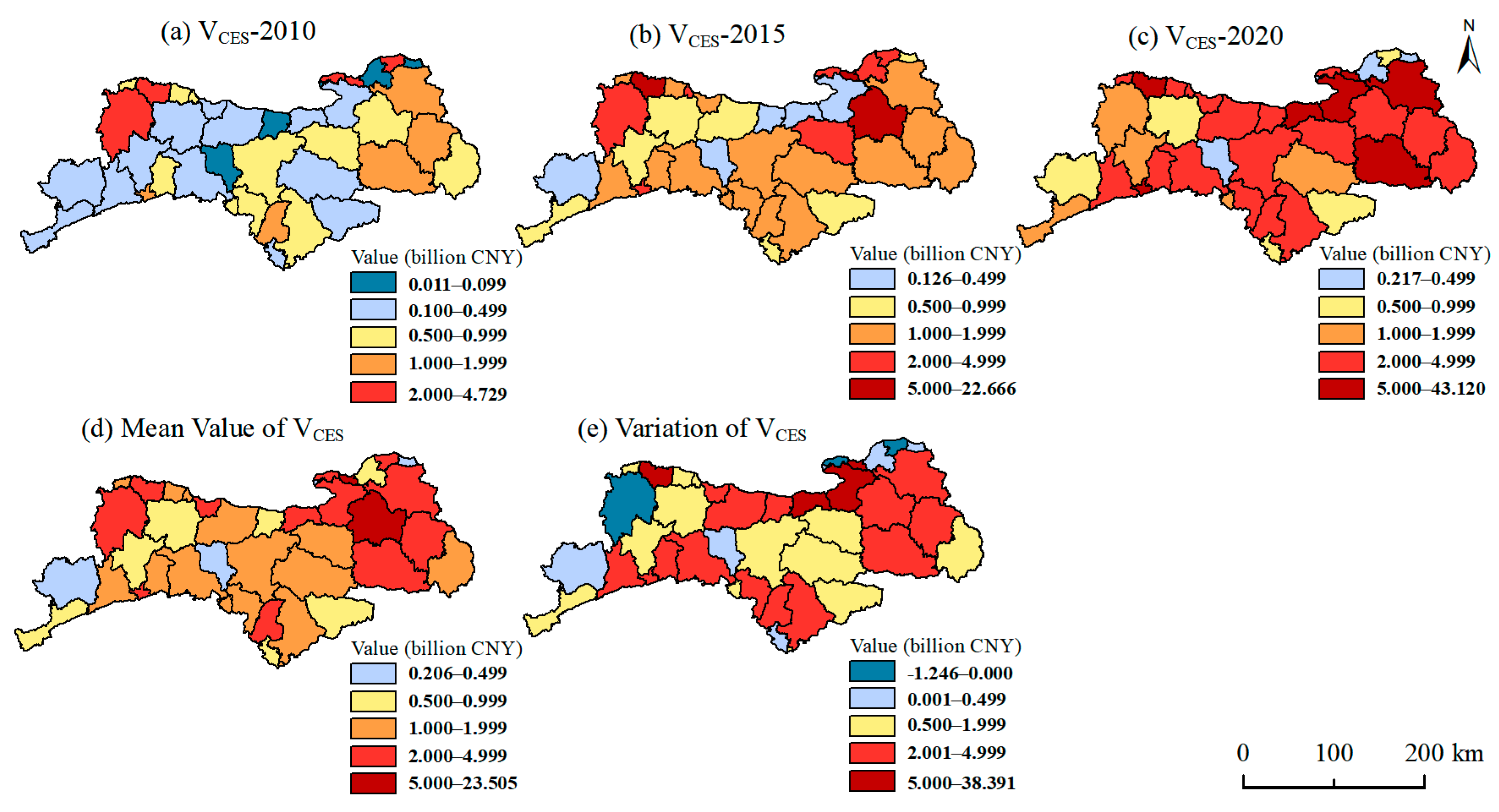
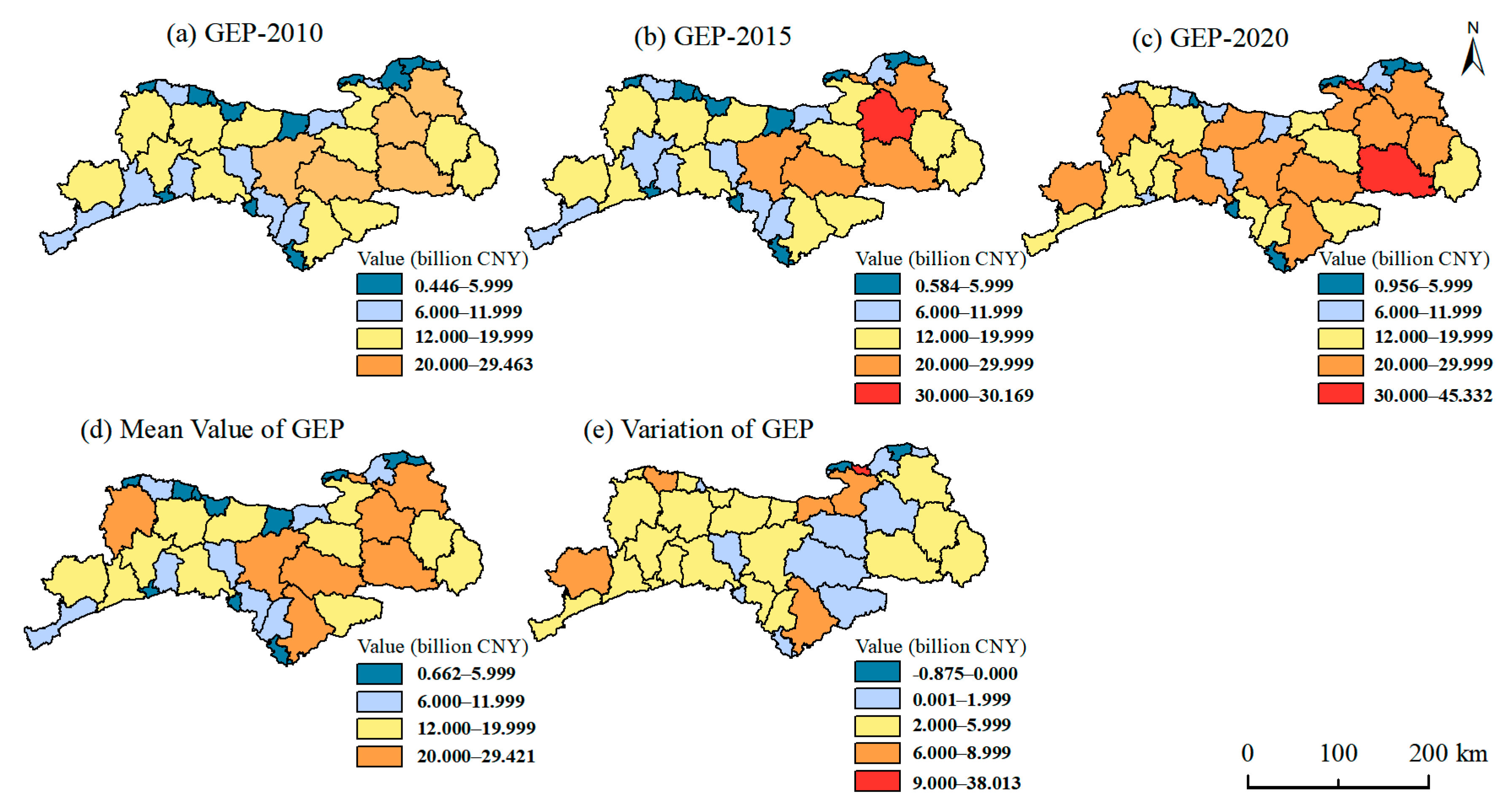
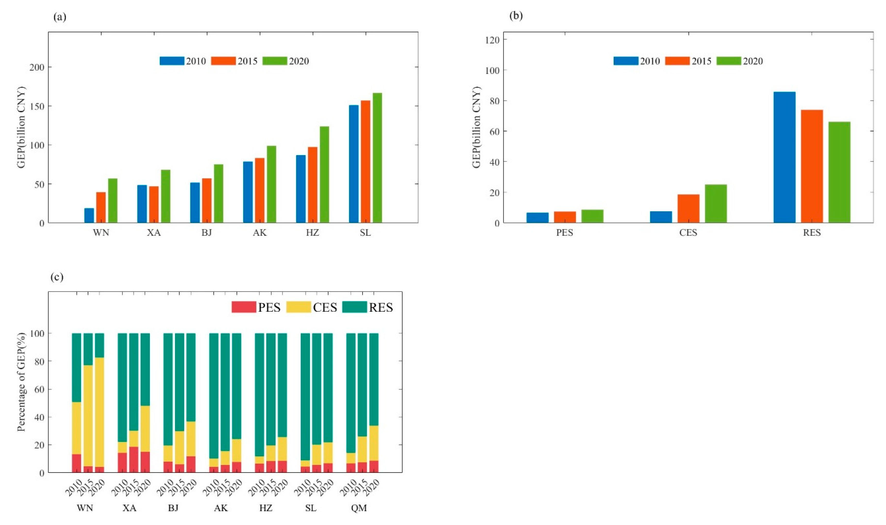
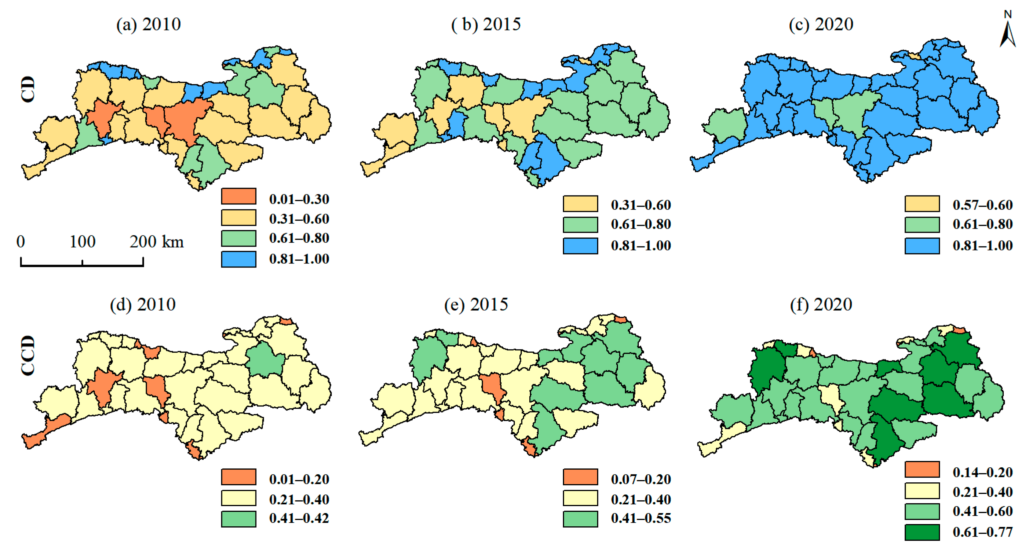

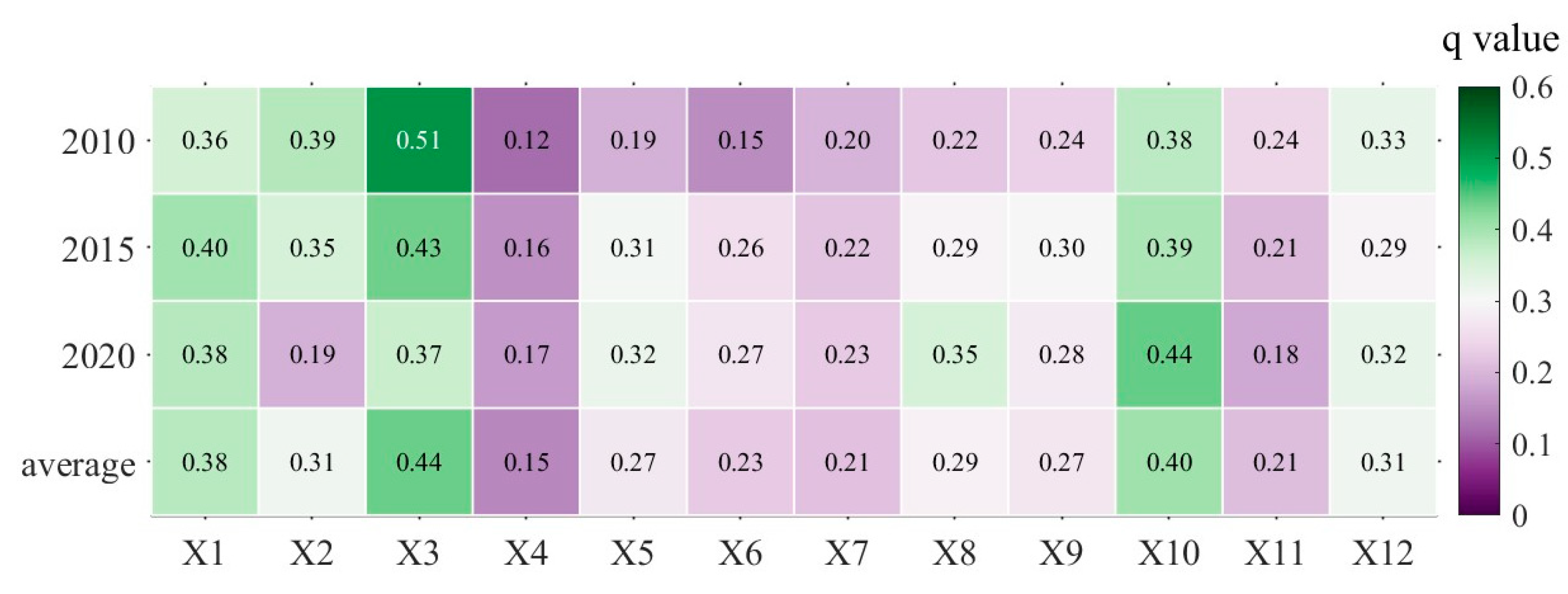

Disclaimer/Publisher’s Note: The statements, opinions and data contained in all publications are solely those of the individual author(s) and contributor(s) and not of MDPI and/or the editor(s). MDPI and/or the editor(s) disclaim responsibility for any injury to people or property resulting from any ideas, methods, instructions or products referred to in the content. |
© 2024 by the authors. Licensee MDPI, Basel, Switzerland. This article is an open access article distributed under the terms and conditions of the Creative Commons Attribution (CC BY) license (https://creativecommons.org/licenses/by/4.0/).