Abstract
The ecological environment in loess hilly regions is fragile, and the contradiction between the development of human society and ecological environment protection is becoming more and more prominent with the intensification of human interference. In order to give full play to the role of ecosystem adaptation in ecological restoration, this study seeks natural conditions that are suitable for the stable existence of ecosystems in the Wanhuigou catchment using the reference ecosystem method and uses these conditions as constraints of the GeoSOS-FLUS model for multi-scenario simulation. Based on ecosystem service value and ecological compensation mechanisms, the comprehensive benefits of different scenarios are compared, and economic development is taken into account while ensuring that ecological protection remains a priority. The results show the following: (1) The unstable ecosystems concentrated on a gentle slope (5–15°) at altitudes of 1201–1379 m, 1201–1594 m, 1379–1715 m and 1715–1856 m are suitable for restoration to farmland, shrub, grassland and forest ecosystems, respectively, and the change characteristics of soil and vegetation communities also verify the above conclusions. (2) The scenario of agricultural development from 2020 to 2030 and the early stages from 2030 to 2050 is the best among the three scenarios, while the scenario of ecological protection is the best in the middle and late stages of 2030–2050. Formulating relevant policies and ecological protection measures according to the scenario of ecological protection is more conducive to promoting the harmonious coexistence of humans and nature. (3) Under the scenario of ecological protection, the unstable ecosystem distributed along the gentle slope (5–15°) of 1379–1483 m and 1483–1594 m achieves the most significant improvement in ecosystem service value by focusing on and giving priority to the restoration of natural conditions that are suitable for the stable existence of ecosystems. This study provides ideas and references for the formation of ecosystem restoration and development strategies for small watersheds in loess hilly regions, and it is of great significance for the promotion of a harmonious coexistence between humans and nature.
1. Introduction
The development mode that sacrifices the environment has led to many serious ecological and environmental problems and has become a bottleneck restricting the development of the social economy. The relationship between the human system and natural ecosystem is both contradictory and unified, and the ultimate goal is to achieve coordination, harmony, order and sustainable development for the two systems [1]. It is necessary to deal with the relationship between environmental protection and economic development, respect nature, comply with nature and protect nature. A development mode based on ecological protection can better preserve ecology and realize the benign interaction between, and mutual transformation of, economic development and ecological protection [2].
Ecological restoration aims to stop human interference in ecosystems in order to reduce load pressure, to rely on the self-regulation and self-organization abilities of ecosystems to allow them to evolve in an orderly direction, or to use the self-recovery ability of ecosystems, supplemented by artificial measures, to gradually restore a damaged ecosystem or help it develop towards a virtuous cycle [3]. The loess hilly region is a key area for large-scale ecological restoration in China. During the process of ecological protection and restoration, it is urgent to explore the internal mechanism of ecosystems, follow the succession law of the natural ecosystem, unleash the self-healing ability of nature, avoid excessive human intervention in the ecosystem and take measures such as protection and restoration, nature and labor, biology and engineering to form the basis of strategies to preserve the natural advantages of ecosystems and promote integrated ecological protection and restoration [4].
Regarding the evolution law of ecosystems, Ouyang et al. [5] used remote sensing combined with a ground survey to obtain the dynamic change information of the national ecological environment from 2000 to 2010 in China, and analyzed the evolution characteristics of the distribution, pattern, quality and ecological service functions over the past 10 years to provide references for the national development strategy and ecological protection supervision. In addition, the relationship between natural factors such as topography, soil and climate, and the evolution laws of ecosystems, are also hot topics for scholars to explore. For example, Fu et al. [6] used canonical analyses (CCA) to study the relationship between a small watershed ecosystem pattern and the slope and soil types in a semi-arid hilly region of the Loess Plateau and pointed out that the farmland ecosystem was mainly distributed over a gentle slope with fertile soil, while grassland and forest ecosystems were mainly distributed over a steep slope with poor soil. Zhao et al. [7] took the Baota District in the middle of the Loess Plateau as the focus of their discussion and used fractal theory to explore the spatial distribution structure characteristics of various ecosystem types. The research showed that the elevation, slope and topographic position were important factors in the formation of an ecosystem distribution pattern. Ecosystem adaptation refers to the process by which ecosystems adjust their structure and function in response to natural environmental changes and biological components interact with environmental factors to continuously adapt to environmental changes [8]. Ecosystem stability is the basis of this adaptation, and the restoration or reconstruction of ecosystems should first maintain their stability [9]. Adaptive restoration means that natural ecosystems give full play to their adaptability and constantly adapt to changes in the natural environment under the premise of long-term stability, thereby achieving a positive evolution.
On the basis of determining the evolution law of an ecosystem and the natural conditions suitable for its stable existence, a simulation analysis of ecosystem evolution in different scenarios can provide scientific support for adjustments to an ecosystem’s structure for different purposes and help to achieve high-quality social and economic development in small watersheds. Scholars usually establish and optimize the ecosystem evolution model based on the combination of a spatial simulation model and quantitative prediction model. For example, Liu et al. [10] embedded the objective optimization model and grey prediction model GM (1, 1) into the non-spatial module of the CLUE-S model in order to optimize land-use types under multi-objective demands. In order to simulate and predict the evolution of land use in the Three Gorges Reservoir area, Zhang et al. [11] comprehensively applied cellular automata based on multi-criteria evaluation (MCE) and the CA-Markov model. Cao et al. [12] took the Jintan District of Changzhou City as the research object, comprehensively considered the sustainable land-use goals such as ecological civilization, rural revitalization and urban–rural integration and set three development scenarios, namely natural evolution, economic priority and ecological priority. Through the combined application of a multi-objective programming model (MOP) and GeoSOS-FLUS model, the land-use pattern was further optimized [13], and they proposed that balancing the urban–rural land use and ecological protection and promoting spatial layout balance should be fully integrated into the future development process of this region.
As an important measure to solve the contradiction between ecological protection and economic development, ecological compensation can be used to compare the advantages and disadvantages of different development scenarios and provide scientific basis and guidance for the formulation of government policies and ecological protection compensation measures. Deng et al. [14] used the method of a modified equivalent factor to estimate the ecosystem service values of 310 counties in the old revolutionary base areas along the Long March, then used the method of regional differential ecological compensation estimation to divide and estimate the priority and amount of ecological compensation in this area and discussed the ecological compensation strategy. Miao and Zhao [15] believed that ecological compensation played an important role in balancing economic development and ecosystem service functions in the important ecological function areas; they calculated the ecosystem service values of the Loess Plateau in Longdong from 2000 to 2020 using the equivalent factor method and calculated the amount and priority of ecological compensation for nine counties on this basis. Lin et al. [16] used the environmental impact assessment method and multi-regional input–output model (MRIO) to construct a framework of inter-regional payments for ecosystem services (PES) estimation, including the regional spillover value of ecosystem services and regional transfer value of pollutants, and estimated the inter-regional payment amount of ecosystem services in the Beijing–Tianjin–Hebei (BTH) region.
Most of the previous studies on the multi-scenario simulation of ecosystems have divided different scenarios based on the development goals, without fully considering the adaptability of the ecosystem itself, only considering the improvement of the total value of ecosystem services in the decision-making of different scenarios [17,18]. By the reference ecosystem method, and based on remote-sensing data and vegetation community survey data, this study determines the suitable conditions for the stable existence of ecosystems and takes these conditions as a basis to divide different simulation scenarios. In scenario analysis, the ecological compensation mechanism is introduced to evaluate the comprehensive benefits of different scenarios, which is not only conducive to the natural restoration of ecosystems but also takes into account both ecology and economic development, thus promoting harmony between humans and nature.
2. Materials and Methods
2.1. Study Area
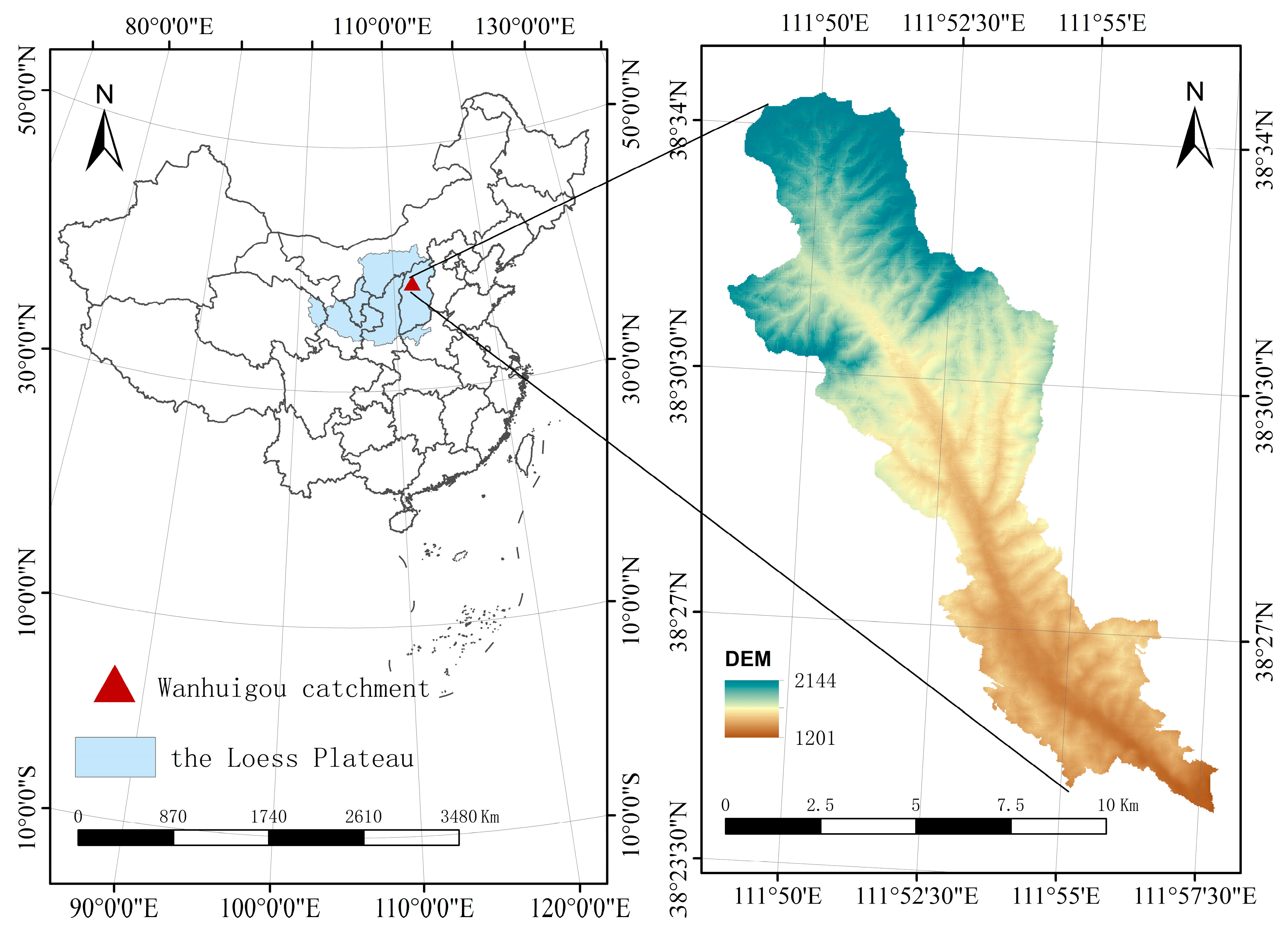
Wanhuigou catchment is located in Jingle County, in the upper reaches of the Fenhe River, and on the Loess Plateau in the northwest of Shanxi Province. The river system Wanhuigou involves is a primary tributary of the Fenhe River. The geographical coordinates are between 111°48′24″–111°57′28″ E and 38°24′45″–38°34′30″ N (Figure 1), and it is close to the county town, with provincial and county roads connected. It involves 12 administrative villages in 2 townships, including Zhangjiazhuang Village, Maquantan Village, Xincun Village, Chaishui Village, Fumatan Village, Zhuangwanggou Village, Maweigou Village, Yaozhuang Village, Dongmafang Village, Laopo Village in Xincun Township, Xiaogoukou Village and Shizuizi Village in Goose Town. Due to the long-term intense soil erosion, the ground has been cut into pieces, and the gully area accounts for 45% of the basin. It belongs to the temperate semi-arid and semi-humid zone in the physical geographical division, the rainfall fluctuates greatly between years and is unevenly distributed throughout the year, and it is highly concentrated in the months from July to September, which is a drought and rainstorm-prone area. The ground is covered by deep loess, and only bedrock is exposed in the ditch. The average annual soil erosion modulus is more than 16,000 t (km2·a), and the soil erosion is serious [19]. Therefore, following the principle of “overall protection, systematic restoration and comprehensive management” and studying a set of technical systems in line with the comprehensive management of ecological environment in the loess hilly regions based on the concept of adaptive restoration will play an important role for the comprehensive management of the ecological environment in this region.

Figure 1.
Location of the study area.
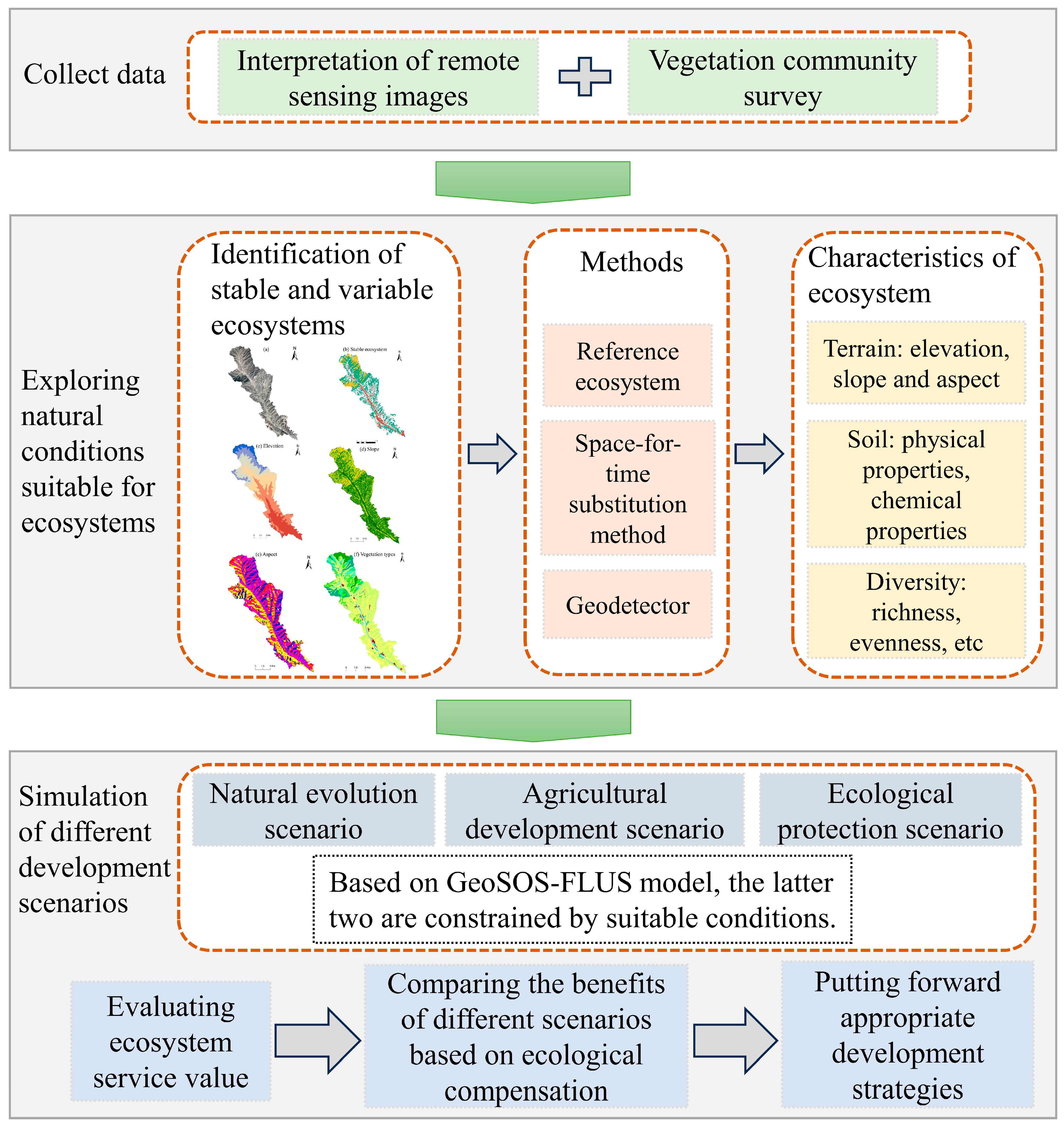
2.2. Research Framework
Based on the interpreted remote-sensing image data, the stable and variable ecosystems are divided according to the stability connotation and change characteristics of ecosystems (the former has no change in ecosystem type from 1985 to 2020, while the latter has changed at least once). Combined with field investigation, the evolution characteristics of the topography, soil and vegetation communities are explored to obtain the natural conditions suitable for the stable existence of ecosystems.
Taking the results above as the limiting conditions, different development scenarios, including the natural evolution scenario, agricultural development scenario and ecological protection scenario, are set up to simulate the ecosystem evolution through a GeoSOS-FLUS model. And based on the ecosystem service value and ecological compensation mechanisms, the comprehensive benefits of ecosystems under different scenarios are compared to provide a reference and scientific basis for the formulation of future policies and ecological restoration measures and to promote the harmonious coexistence between humans and nature (Figure 2).
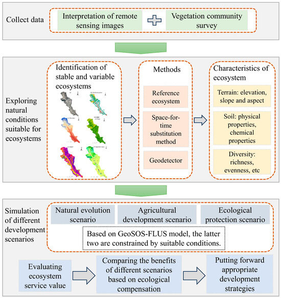
Figure 2.
Framework for the study.
2.3. Data Sources
The ecosystem data from 1985 to 2020 is based on Landsat TM/ETM+/OLI images, and generated through visual interpretation and supervised classification, with an interpretation accuracy of over 85% and a resolution of 30 m × 30 m. The ecosystem classification results are revised according to the three land use status surveys, many years of land use change survey data (provided by the local government) and field surveys. The types of ecosystems in this study include farmland, forest, shrub, grassland and urban ecosystems.
The terrain data include elevation, slope and aspect. The elevation is derived from geospatial data cloud ASTER GDEM 30 M resolution digital elevation data (http://www.gscloud.cn/ accessed on 30 March 2020), and the slope and aspect are extracted from the elevation data through ArcGIS 3D Analyst Tools-Raster Surface. The elevation is divided into six gradients using the natural breakpoint method, respectively represented by Elevations 1–6. According to the technical specification for the investigation and assessment of national ecological status, the slope is divided into six grades, namely flat slope, gentle slope, slope, steep slope, sharp slope and dangerous slope, respectively represented by Slopes 1–6. According to the difference in illumination in each aspect, the aspect is divided into five grades: no aspect, shady aspect, semi-shady aspect, sunny aspect and semi-sunny aspect, which are represented by Aspects 0–4, respectively (Table 1).

Table 1.
Classification of terrain factors.
In the investigation of vegetation community characteristics, the maps of the vegetation community, stable ecosystem, elevation grade, slope grade and aspect are superimposed to determine the location of sample points. In order to make the layout of the sample points represent the whole, the layout covers most of the major vegetation communities, the number and spacing are determined according to the distribution range of vegetation communities and the distance is within a certain range to ensure that the gradient change in environmental factors can be reflected. The survey indicators include species name and number, vegetation coverage, elevation, slope, aspect, soil texture, bulk density, depth, pH, cation exchange capacity, total nitrogen, total phosphorus, total potassium, organic matter content and density. The survey was conducted from April to July 2020.
2.4. Methods
2.4.1. Reference Ecosystem
An ideal reference ecosystem is composed of specific values of a series of key indicators that reflect the quality of the ecosystem under suitable environmental conditions, with no or little human interference, and the key indicators mainly include those that can directly or indirectly reflect the composition, structure and function of ecosystems [20]. Ecosystems in the same ecoregion that are less disturbed by human activities and more affected by climatic factors can be selected as reference ecosystems according to the law that key indicators or parameters of the same ecosystem type are similar under the same or similar natural environment conditions [21].
In this paper, the ecosystem whose type has not changed for many years (i.e., stable ecosystem) is regarded as the reference ecosystem. Based on remote-sensing image data, the topographic characteristics of the stable ecosystem are analyzed, and the characteristics of soil and vegetation diversity are obtained based on vegetation community survey data. The comprehensive characteristics of the topography, soil and vegetation are used to guide the restoration direction of variable ecosystems.
2.4.2. GeoSOS-FLUS Model
This study uses the GeoSOS-FLUS model to simulate the future changes in the ecosystem pattern. It is an effective model for geospatial simulation, spatial optimization and decision-making assistance [13]. Some studies have shown that the simulation accuracy of the GeoSOS-FLUS model is higher than that of CLUE-S, artificial neural networks (ANNs), cellular automata (CA) and other models [22]. The model firstly uses ANN to obtain the suitability probability of various types of land use and then improves the applicability of the model using a coupling system dynamics model (SD) and CA. In the CA model, an adaptive inertial competition mechanism is introduced to deal with the complexity and uncertainty of the mutual transformation of various land-use types under the joint influence of nature and human activities.
In order to explore the development path between humans and nature, according to the principles of unifying economic and ecological benefits, and balancing protection and utilization, with 2030 as the target year, three development scenarios are set to simulate the ecosystems:
Scenario 1: Natural development scenario. Also known as the inertial development scenario, it is based on the change rate of ecosystem pattern from 1985 to 2020, combined with historical natural and human-driven factors, without considering policy planning constraints, and it predicts the future scale of each ecosystem through the grey Markov model and serves as the scale demand parameter for the FLUS model, which is the basis for the other scenarios.
Scenario 2: Agricultural development scenario. With the priority of economic benefits as the objective, the probability of other ecosystems transforming into urban and farmland ecosystems should be appropriately increased with reference to relevant planning and policies under the premise of following the laws of nature, and variable ecosystems suitable for both farmland and grassland should be restored to farmland as much as possible.
Scenario 3: Ecological protection scenario. The priority of ecological benefits is the optimization goal, strengthening the protection of ecological land, and variable ecosystems that are suitable for both farmland ecosystem and ecological protection should be restored to ecosystems that are conducive to ecological protection as much as possible.
2.4.3. Estimation of Ecosystem Service Value
The evaluation methods for ecosystem service value mainly include the functional value method based on the unit service functional price and the equivalent factor method based on the unit area value [23]. This study uses the equivalent factor method to calculate the ecosystem services value, and the basic equivalent scale is updated and improved by Xie Gaodi [24]. The value of various service functions and the total service function value of the ecosystem are calculated based on the area of various ecosystems, and the formula is as follows:
where is the value of the -th ecosystem service function in the -th ecosystem, is the value of the -th ecosystem service function, represents the value of the -th ecosystem service functions, represents the total value of the ecosystem service functions, is the value coefficient of the -th ecosystem service function in the -th ecosystem, is the area of the -th ecosystem, is the number of ecosystem types and is the number of ecosystem service function items.
The functional intensity of different types of services is influenced by different ecological conditions and processes. Therefore, this study used three types of data, namely net primary productivity (NPP), rainfall and soil conservation, to revise the basic equivalent scale of ecosystem service value, so as to accurately reflect the changes in ecological service functions and their value in different regions on spatial dimension. And the values of the ecosystem service functions per unit area in the study area are shown in Table 2.
Table 2.
The value of ecosystem service functions per unit area in the study area (CNY/hm2·a).
2.4.4. Ecological Compensation
The ecological compensation mechanism is the internalization of the economic externalities of ecological protection behavior, that is, the cost paid by ecological builders for protecting the ecological environment is compensated by making the beneficiaries of ecological protection achievements pay corresponding fees, so that ecological protectors can enjoy the economic benefits brought by their ecological protection achievements. This mechanism is conducive to improving the fairness between producers and consumers of special “public goods” such as ecological service function, ensuring that investors of ecological function can obtain reasonable returns, positively encouraging the sustainable production of ecological service function products and achieving harmonious coexistence between humans and nature [25].
In order to improve the practical feasibility and operability of ecological compensation standards, this study calculates the total value of regional ecosystem services through the research results of Costanza [23] and Xie Gaodi et al. [24], as well as land-use data, and uses socio-economic coefficients to correct them, thus obtaining a feasible ecological compensation standard. Engel’s coefficient can measure the living standard of human beings, the Pearl growth model has the same changes with humans’ understanding of ecosystem service functions and incorporating Engel’s coefficient into the Pearl growth model can better reflect the level of socio-economic development. The formula is as follows:
where is the development stage coefficient of year , is the Engel’s coefficient of year , is the base of natural logarithm, is the food expenditure of year and represents the total consumption expenditure of year .
3. Results
3.1. Natural Conditions Suitable for Ecosystems in Different Situations
Through the factor detection and interaction detection analysis of geographical detectors (GeoDetector), it is found that elevation and slope play a major role in the topographic differentiation of ecosystems. Therefore, a thorough analysis is conducted on the topographic combination conditions of elevation and slope. The area of stable farmland ecosystems distributed in “elevation 1-slope 2” accounted for the largest proportion of stable farmland ecosystems, which is 29.47%. The area proportion of stable forest ecosystems distributed in “elevation 5-slope 3” is the highest, at 20.19%. The proportion of stable shrub ecosystems distributed in “elevation 3-slope 2”, “elevation 2-slope 2” and “elevation 1-slope 2” ranks in the top three, with 18.51%, 17.49% and 11.56%, respectively. The proportion of stable grassland ecosystems distributed in “elevation 3-slope 2”, “elevation 4-slope 2” and “elevation 2-slope 2” ranks in the top three, with areas of 16.28%, 14.40% and 11.55%, respectively. And the proportion of stable urban ecosystems distributed in “elevation 1-slope 2” and “elevation 1-slope 1” ranks in the top two, at 42.73% and 27.28%, respectively (Table 3).
Table 3.
Area proportion of stable ecosystems under different combination conditions of elevation and slope.
Through the numerical analysis of soil physical and chemical properties (Table 4), it can be seen that the soil properties of the variable ecosystems distributed in “elevation 1-slope 2” are close to those of stable farmland ecosystems. Among them, clay, silt, tk and tp are 15.42 g/100 g, 36.708 g/100 g, 15.719 g/kg and 0.451 g/kg, respectively, which are lower than those of stable farmland ecosystems, sand is 47.846 g/100 g, which is higher than that of stable farmland ecosystems, and the others are basically the same as those of stable farmland ecosystems. The soil properties in the variable ecosystems of “elevation 2-slope 2” are close to those of stable farmland ecosystems, and there is a tendency to shift to the soil physical and chemical properties suitable for constructing stable grassland ecosystems. The soil properties of variable ecosystems distributed in “elevation 3-slope 2” are close to those of stable grassland ecosystems, and the pH is 8.009, which is between stable farmland and grassland ecosystems, while the others are relatively similar to stable grassland ecosystems. The CEC of variable ecosystems distributed in “elevation 4-slope 2” is 181.477 mmol/kg, which is close to the Pinus tabulaeformis community in stable forest ecosystems; clay is 19.335 g/100 g, which is close to the spruce community; tk is 17.716 g/kg, which is between Pinus tabulaeformis community and stable shrub ecosystems; and the others are close to stable shrub ecosystems.
Table 4.
Comparison of soil properties between variable and stable ecosystems under dominant elevation–slope conditions.
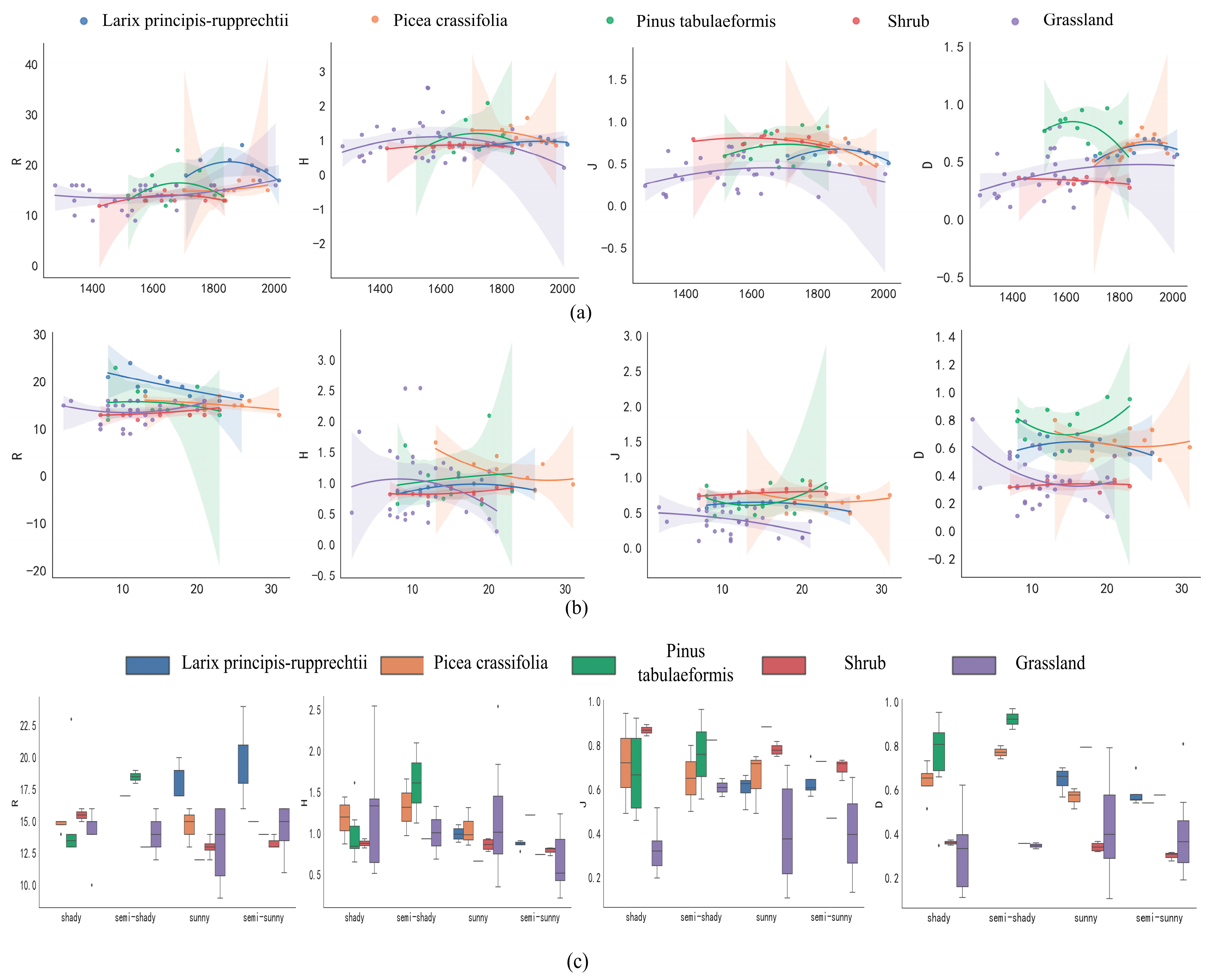
The forest ecosystem at an altitude of 1718–2128 m is suitable for using North China larch as the constructive species, and this community can be restored and constructed based on the rules of high species richness and evenness at altitudes of 1900–2000 m and slopes of 15–20°, low at around 1700 m and 2100 m and on flat and steep slopes and suitable distribution on sunny or semi-sunny aspects. At an altitude of 1660–1980 m, spruce is suitable as the constructive species, and the community can be restored or constructed according to the law of low species richness and high evenness at 1800–1900 m, high species richness and low evenness at 1700 m and 2000 m, high species richness on gentle slopes, low evenness on slopes of 20–25° and high evenness on gentle and steep slopes, as well as suitable distribution on sunny and shady aspects. It is suitable to take Pinus tabulaeformis as the constructive species at an altitude of 1530–1900 m, and the community can be restored or constructed based on the law of high species richness and evenness at 1690–1790 m, low at around 1550 m and 1900 m, high evenness on gentle and steep slopes, small on slopes of 12–16° and suitable distribution on shady and semi-shady aspects. Adaptive shrub ecosystems can be constructed at an altitude of 1403–1879 m, specifically according to the law that species richness and evenness are high at 1600–1700 m, but low at around 1450 m and 1850 m, and it is suitable for distribution on sunny and semi-sunny aspects. Adaptive grassland ecosystems can be constructed at an altitude of 1276–2108 m, specifically according to the law that species richness is low and evenness is high at 1600–1800 m, but it is the opposite at 1300 m and 1900 m, and species richness is low at a slope of 10–15° and high on gentle and steep slopes, and it is suitable for distribution on sunny and semi-sunny aspects (Figure 3).
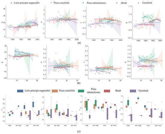
Figure 3.
Variation in species diversity index of different vegetation communities with topographic gradients. (a–c) represent the changes in species diversity indices of different vegetation communities with elevation, slope, and aspect, respectively. R, D, H and J represent four species diversity indices, namely the species richness index, Simpson dominance index, Shannon–Wiener diversity index and Pielou evenness index.
3.2. Multi-Scenario Simulation Based on GeoSOS-FLUS Model
Based on the ecosystem data of the study area in 2015, the simulation results of the ecosystems in 2020 are obtained. The test results shows that the Kappa coefficient is 0.7740, and the overall accuracy reaches 89.01%. The simulation results are basically consistent with the actual distribution in space, and the simulation effect is good, which can be used to predict the future changes in ecosystem pattern.
With 2020 as the forecast base year, the ecosystem area in 2030 is predicted. The simulation results (Figure 4) show that under the natural development scenario, the spatial layout of the ecosystem is relatively stable and grassland is still the main ecosystem type, with its area increased somewhat. The increase in the urban ecosystem area is mainly concentrated in the surrounding areas of cities, where the level of economic development is high, the demand for production and living land is large and the traffic location advantage is obvious. In both the agricultural development scenario and the ecological protection scenario, the area of forest, grassland and urban ecosystems increases, while those of the farmland and shrub ecosystems decreases. Under the agricultural development scenario, the reduction in the farmland ecosystem area and the increase in the grassland ecosystem area are relatively small. In the ecological protection scenario, there is a significant decrease in the area of farmland ecosystems and an increase in the area of grassland ecosystems, while the area of other types of ecosystems changes little. The decrease in farmland ecosystems is mostly in the steep slope area with a higher altitude, and the increase in the grassland ecosystem area comes partly from areas with higher elevations and steep slopes and partly from areas with lower elevations and gentle slopes. For areas with a low altitude and gentle slope, under the premise of optimizing the ecosystem pattern based on environmental factors, the agricultural development scenario focuses on developing farmland ecosystems, while the ecological protection scenario focuses on developing grassland ecosystems.
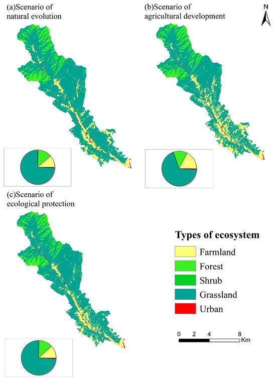
Figure 4.
Simulation results of ecosystems in different scenarios in 2030.
3.3. Ecosystem Service Value in Different Scenarios
Through the evaluation of the ecosystem service value and the study of ecosystem pattern change, the ecosystem service values in different scenarios from 2030 to 2050 is obtained (Table 5). Under a natural evolution scenario, the ecosystem service value of the study area increases from CNY 327.96 million in 2030 to CNY 427.27 million in 2050, with a total increase of CNY 99.31 million. Under the agricultural development scenario, the ecosystem service value in 2050 is approximately CNY 427.38 million, which is CNY 100.93 million higher than that in 2030, and the total service value is slightly higher than that in the natural evolution scenario. Under the ecological protection scenario, the ecosystem service value in 2050 is about CNY 442.59 million, an increase of CNY 103.21 million compared with 2030, which is significantly higher than the other two scenarios. The ecosystem service value of ecological protection scenario is CNY 15.21 million higher than that of the agricultural development scenario in 2050.
Table 5.
Value of ecosystem services in different scenarios. (Unit: ten thousand yuan).
3.4. Comprehensive Benefits of Different Scenarios Based on Ecological Compensation Mechanisms
By evaluating the ecosystem service value in different scenarios, the comprehensive benefits of different development strategies can be compared and analyzed in combination with ecological compensation mechanisms, which provides a scientific basis for selecting future development strategies and formulating ecological protection measures [26,27].
In 2030, the ecosystem service value of the ecological protection scenario is CNY 12.93 million more than that of the agricultural development scenario. After correction, the compensation difference is CNY 6.99 million, while the economic value generated by a farmland ecosystem in the agricultural development scenario is CNY 7.35 million more than that in the ecological protection scenario. Compared with the natural evolution scenario, the agricultural development scenario is similar in ecological compensation, while the farmland ecosystem produces more economic benefits. Therefore, the agricultural development scenario in 2030 is the optimal scenario.
4. Discussion
4.1. Adaptive Restoration of Ecosystems
Referring to the distribution characteristics of stable ecosystems under different terrain conditions, and superimposing the maps of ecosystem types and terrain factor gradients for many years, it can be seen that the variable ecosystem distributed in “elevation 1-slope 2” is suitable to be restored to a farmland ecosystem, while the variable ecosystem distributed in “elevation 2-slope 2” is suitable for restoration to farmland, grassland and shrub ecosystems, or even a forest ecosystem, and the variable ecosystems distributed in “elevation 3-slope 2” and “elevation 4-slope 2” are suitable for restoration to grassland, shrub, and forest ecosystems (Table 3) [19].
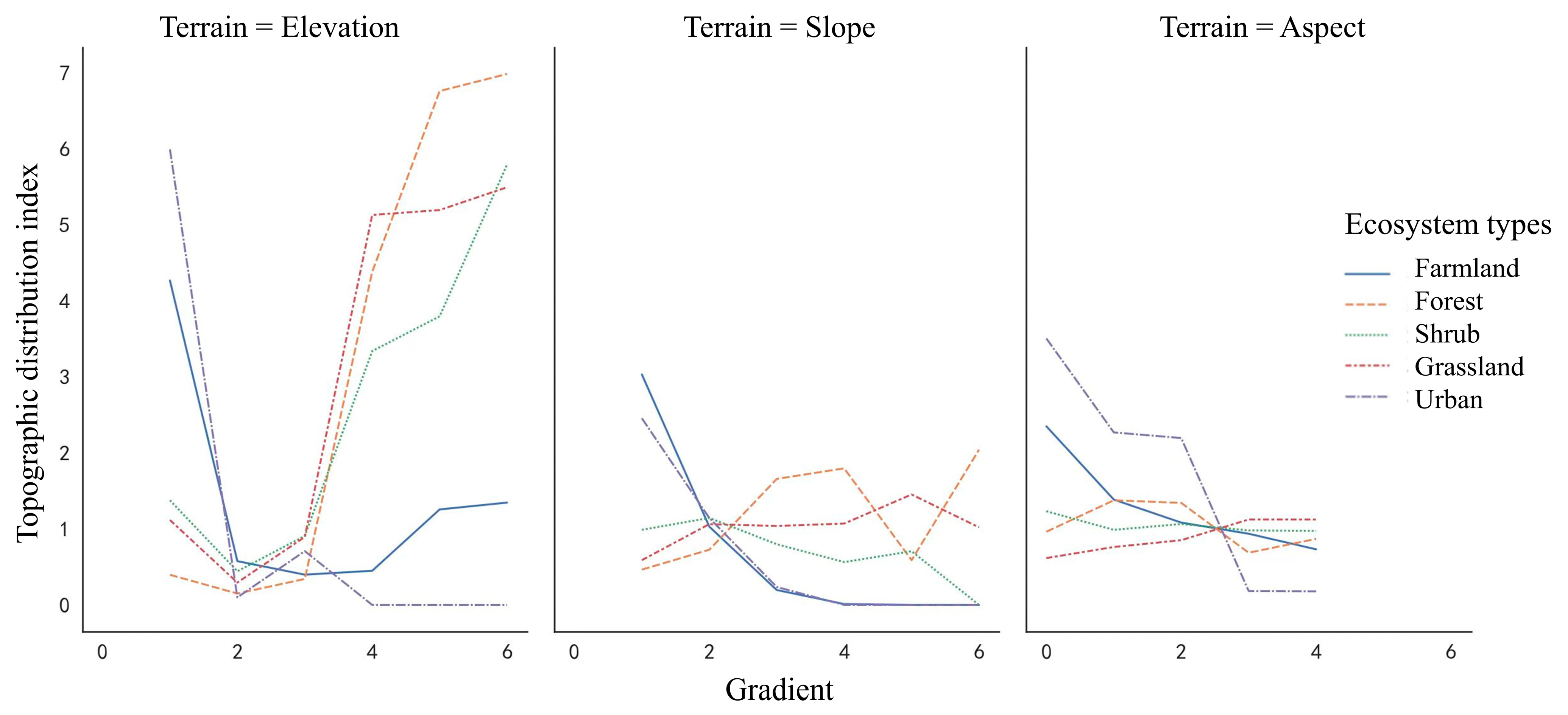
In order to effectively eliminate the area interference of ecosystem types in topographic gradient intervals, the topographic distribution index is used to analyze various stable ecosystems to verify the rationality of pattern adjustment. The dominant ecosystem at Elevation 1 is stable farmland ecosystem, which has greater advantages than other stable ecosystems. At Elevations 2 and 3, the dominant degree of stable ecosystems is similar, with stable farmland, shrub, grassland, and forest ecosystems in descending order. At Elevations 4, 5 and 6, stable forest ecosystems gradually occupy a distribution advantage, followed by stable grassland and shrub ecosystems, and stable farmland ecosystems have the lowest degree of dominance. The characteristics of dominance degree of each stable ecosystem on the slope gradient are similar to those of the elevation gradient, but the difference in the dominance degree compared to the elevation gradient is relatively small (Figure 5) [28]. Through the analysis of the distribution index of stable ecosystems, and combined with the changing patterns of dominant position of ecosystems in different periods, the above adjustment strategies for variable ecosystem types are reasonable [29].
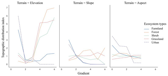
Figure 5.
Topographic distribution index of different ecosystem types on topographic gradients.
The comparative analysis of soil properties between variable and stable ecosystems under different terrain combinations shows that the soil physical and chemical properties of variable ecosystems are similar to those of stable farmland ecosystems, followed by stable grassland ecosystems, and significantly different from stable shrub and forest ecosystems (Table 4). This indicates that it is easier to transform the variable ecosystems into stable farmland and grassland ecosystems but more difficult to transform them into stable shrub and forest ecosystems. On the basis of suitable terrain combination conditions, soil improvement is a prerequisite for transforming an ecosystem into a stable shrub or forest ecosystem [30].
For specific environmental conditions, after constructing suitable terrain and soil conditions, the biological parts of ecosystems can be further constructed and configured according to the characteristics of community species diversity and the law of vegetation succession [31,32], so as to ultimately realize the restoration and construction of different ecosystems with biodiversity, strong stress resistance and stability [33].
4.2. Comparison of Ecosystem Service Value
4.2.1. Comparison of Comprehensive Benefits of Ecosystems under Different Scenarios
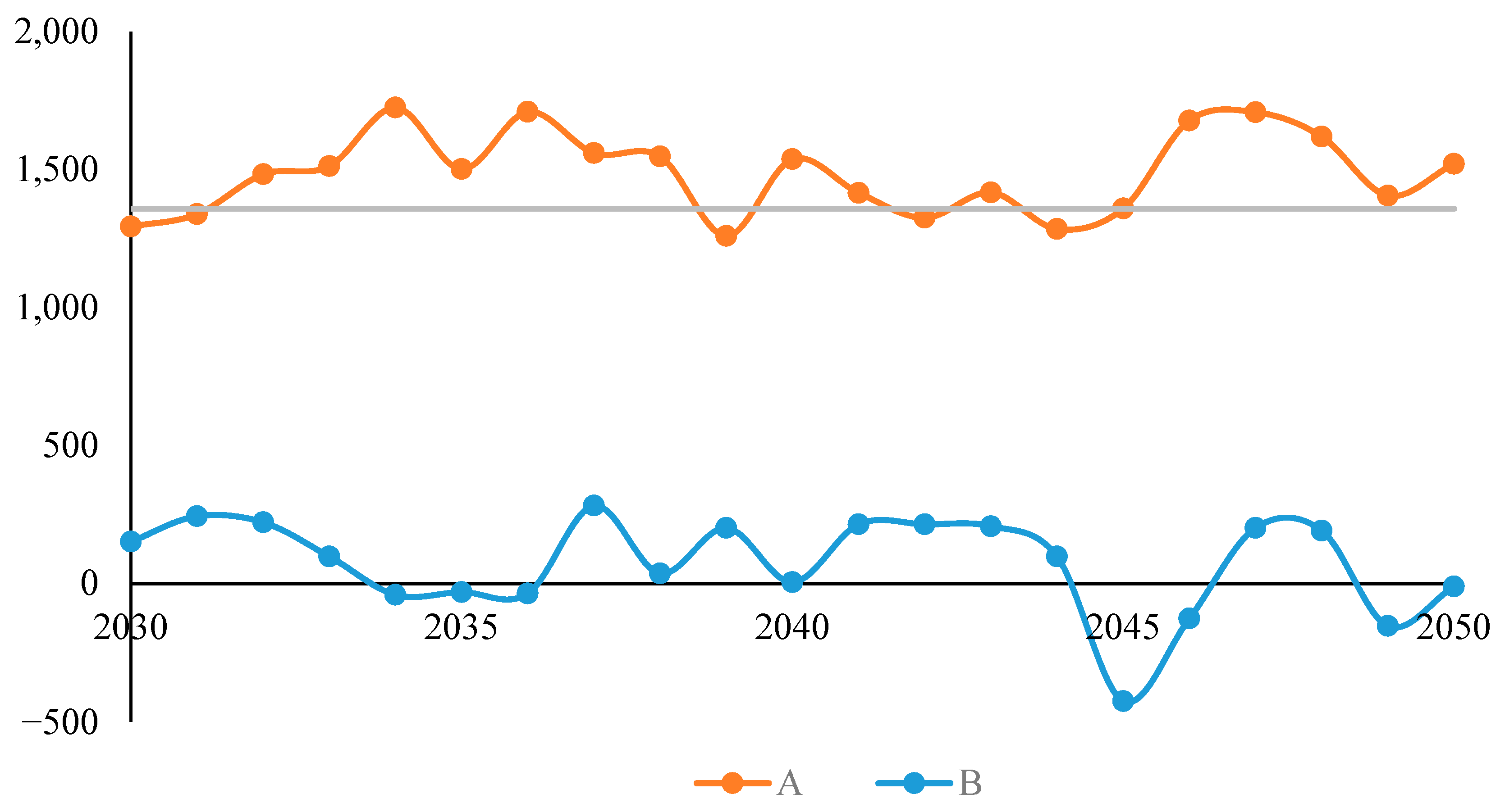
In order to further explore the difference in ecosystem service value in different scenarios, two groups of differences are calculated respectively, that is, A: The difference between the ecosystem service value in the ecological protection scenario and the ecosystem service value in the agricultural development scenario. B: The difference between the ecosystem service value under the natural evolution scenario and the ecosystem service value under the agricultural development scenario. It can be seen that in most years from 2030 to 2044, the ecosystem service value in the natural evolution scenario is higher than that in the agricultural development scenario, and it tends to be consistent around 2035, 2038 and 2040, while the ecosystem service value of the agricultural development scenario tends to be higher than that of the natural evolution scenario from 2045 to 2050 (Figure 6). In addition, the area of the farmland ecosystem under the agricultural development scenario is larger than that under the natural evolution scenario, and its economic benefits are also greater than that under the natural evolution scenario, so the comprehensive benefits under the agricultural development scenario are better than those under the natural evolution scenario [34].
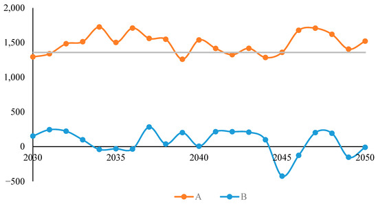
Figure 6.
Difference in the ecosystem service value under three scenarios.
Only when the ecosystem service value under the ecological protection scenario exceeds that of the agricultural development scenario by CNY 13.59 million, and after the correction of the socio-economic coefficient, can the economic benefits generated by a farmland ecosystem under the agricultural development scenario be exceeded [35]. As can be seen from Figure 6, A is less than CNY 13.59 million at the beginning of 2030, and gradually greater than CNY 13.59 million later. In the process of fluctuation, except for a few years below the threshold value, the others are above the threshold value. Therefore, in 2020–2030 and the early stage of 2030–2050, the agricultural development scenario is superior to the ecological protection scenario, and the ecological protection scenario is better in the middle and later stages from 2030 to 2050. The main reason is that compared with the agricultural development scenario, the ecological protection scenario is conducive to the stability of ecosystems in the study area [36], which not only enhances the adaptability of ecosystems to climate change but also ensures the income of farmers on the premise of reducing human interference [37].
4.2.2. Restoration Effects of Different Natural Conditions under Ecological Protection Scenario
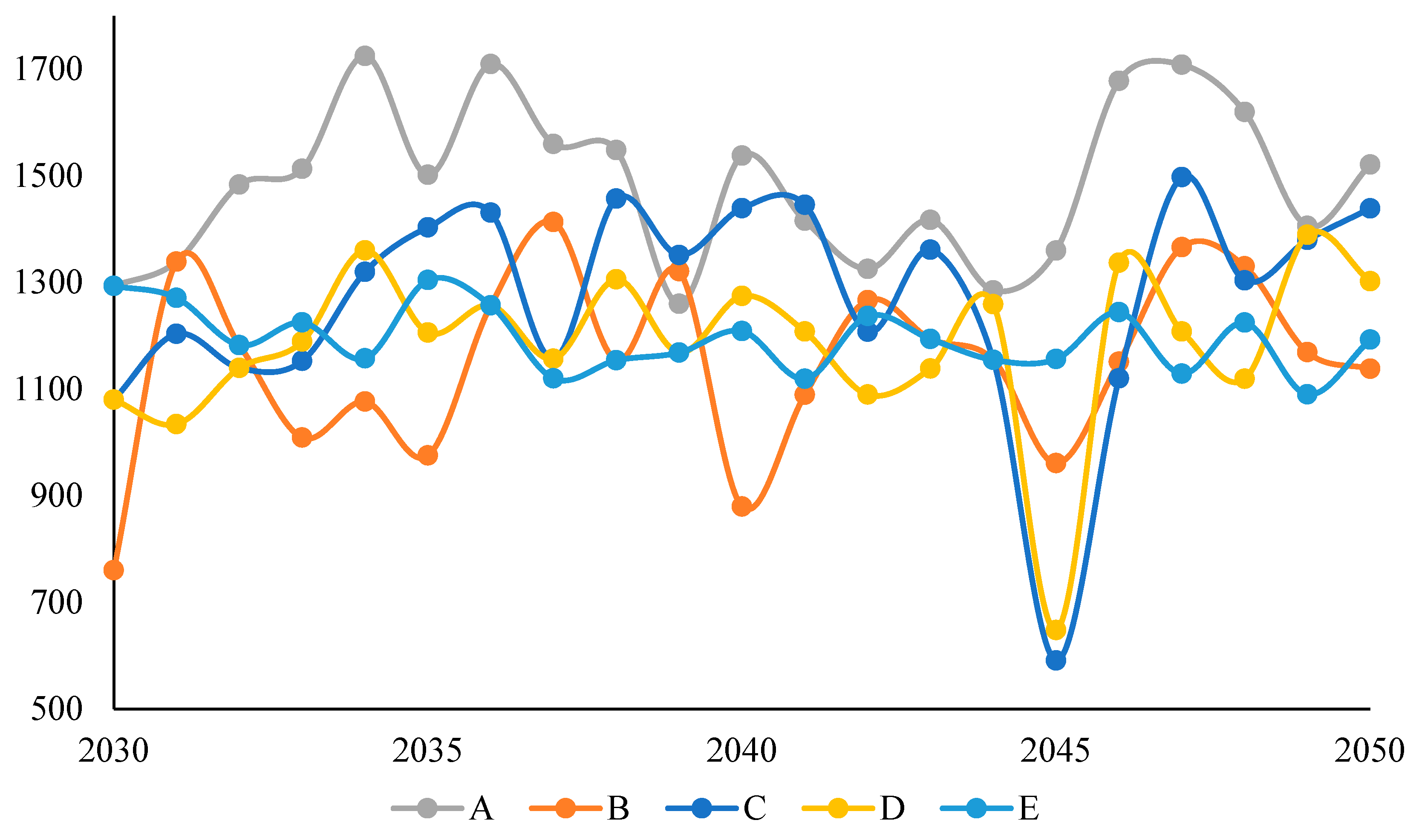
In order to further analyze the restoration effects of different natural conditions under the ecological protection scenario, the ecosystem service value under specific natural conditions is compared with that of the agricultural protection scenario, namely A: The difference in the ecosystem service value between the ecological protection scenario and the agricultural development scenario. B: “elevation 1-slope 2” is the ecological protection scenario, and the rest of the terrain combinations represent the natural evolution scenario. B represents the difference in the ecosystem service value in this scenario and in the agricultural development scenario. C: “elevation 2-slope 2” is the ecological protection scenario, and the rest of the terrain combinations represent the natural evolution scenario. C represents the difference in the ecosystem service value in this scenario and in the agricultural development scenario. D: “elevation 3-slope 2” is the ecological protection scenario, and the other terrain combinations are natural evolution scenarios. D represents the difference in the ecosystem service value in this scenario and in the agricultural development scenario. E: “elevation 4-slope 2” is the ecological protection scenario, and the rest of terrain combinations represent the natural evolution scenario. E represents the difference in the ecosystem service value in this scenario and in the agricultural development scenario.
On the whole, the difference in the ecosystem service value of A is the largest, followed by C and D, and the difference in B and E is smaller, with B and C fluctuating sharply, while C and D fluctuate relatively smoothly (Figure 7). The area of “elevation 1 to slope 2” suitable for restoration to a grassland ecosystem is relatively large, due to significant human interference; the restoration of its ecological function is not ideal, resulting in lower ecosystem service value and greater fluctuation [38]. “elevation 4-slope 2” is suitable for restoration to forest or shrub ecosystems with a larger area, less human disturbance and less fluctuation in the ecosystem service value; due to the small restoration area, the ecosystem service value is not high [39]. Compared with “elevation 1-slope 2”, “elevation 2-slope 2” has a larger area suitable for restoration and more suitable for restoration into shrub and forest ecosystems with less human interference, so its ecosystem service value is greater than that of “elevation 1-slope 2”. Although the area suitable for restoration in “elevation 3-slope 2” is not as large as that of “elevation 2-slope 2”, it has a larger area suitable for restoration to shrub and forest ecosystems, and it is less affected by human interference, resulting in a high ecosystem service value and relatively gentle fluctuations. In summary, in the formulation of ecological protection measures, priority can be given to restoring the areas of “elevation 2-slope 2” and “elevation 3-slope 2”.
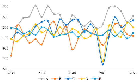
Figure 7.
Comparison of restoration effects of different natural conditions under ecological protection scenarios.
4.3. Innovation and Uncertainty
Based on the adaptive management strategy of the micro-watershed ecosystem, combined with the ecological compensation mechanism, this study compares and analyzes the comprehensive benefits of ecosystem patterns under different development strategies. It comprehensively considers the restoration or construction of adaptive ecosystems and the socio-economic development of the micro-watershed and attempts to explore the path of harmonious development between humans and nature.
However, there are many factors that affect the evolution and spatial layout of ecosystems, coupled with the complexity of the research object, and there are still some elements that have not been fully considered. Therefore, the selected indicator system for influencing factors will be improved based on the actual monitoring results in the future, so as to further improve the simulation accuracy, make it more reasonable and scientific and better meet the actual needs [40]. In addition, further improvements and modifications need to be made in the correction of the ecosystem service value, measurement of socio-economic level and economic benefits of farmland ecosystems in combination with the actual situation of future changes [41]. Adaptive management can be continuously evaluated, demonstrated, improved, and adjusted to make predictions and research results more accurate and reasonable and provide more scientific guidance and support for government decision-making.
5. Conclusions
Nowadays, the contradiction between human development and environmental protection is becoming increasingly prominent, and it is urgent to seek a path of harmonious development between humans and nature. Based on remote-sensing image and vegetation community survey data, this study has revealed the natural conditions suitable for the stable existence of different ecosystems through the concept of a reference ecosystem. By comprehensively comparing the characteristics of topography, soil and vegetation, it is found that unstable ecosystems distributed along gentle slopes (5–15°) at altitudes of 1201–1379 m, 1201–1594 m, 1379–1715 m and 1715–1856 m are suitable for restoration to farmland, shrub, grassland and forest ecosystems, respectively. A comparison of soil physical and chemical properties in different ecosystems shows that it is easier to transform variable ecosystems into stable farmland and grassland ecosystems but more difficult to transform them into stable shrub and forest ecosystems. On the basis of suitable terrain combination conditions, soil improvement is a prerequisite for transforming into stable shrub and forest ecosystems. For specific environmental conditions, the biological components of ecosystems can be further constructed and configured according to the characteristics of community species diversity and the law of vegetation succession.
Taking the conditions suitable for the stable existence of ecosystems as constraints for multi-scenario simulation of the GeoSOS-FLUS model, the simulation results show that the area of forest, grassland and urban ecosystems increases, while that of farmland and shrub ecosystems decreases in both the agricultural development scenario and ecological protection scenario. By further comparing the comprehensive benefits of the natural evolution scenario, agricultural development scenario and ecological protection scenario combined with an ecosystem service value evaluation and ecological compensation mechanism, it is found that the agricultural development scenario is the optimal among the three scenarios from 2020 to 2030 and the early stage of 2030 to 2050, while the ecological protection scenario will become the best in the middle and late stage from 2030 to 2050. In the long run, it is recommended to choose the ecological protection scenario as the direction for the future development of the study area; this not only helps to enhance the adaptability and stability of ecosystems but also ensures the income of farmers in the study area under the prerequisite of reducing human interference, which is conducive to realizing the harmonious coexistence of humans and nature. Under the ecological protection scenario, the unstable ecosystems distributed along the gentle slope (5–15°) of 1379–1483 m and 1483–1594 m have the most significant improvement in ecosystem service value by focusing on and giving priority to restoration according to the natural conditions suitable for the stable existence of ecosystems.
Author Contributions
Conceptualization, Q.L., X.S. and Z.Z.; data curation, Q.L. and Q.W.; funding acquisition, Q.L. and X.S.; investigation, Q.L.; methodology, Q.L., X.S., Z.Z. and Q.W.; resources, Q.L. and Z.Z.; software, Q.L. and Q.W.; supervision, X.S. and Z.Z.; visualization, X.S., Z.Z. and Q.W.; writing—original draft, Q.L. and Q.W.; writing—review and editing, Q.L. and Q.W. All authors have read and agreed to the published version of the manuscript.
Funding
This research was funded by the Doctoral Scientific Research Foundation of Jiangxi University of Science and Technology [grant number 205200100704] and the Charity Special Project of Ministry of Land and Resources of the People’s Republic of China [grant number 201411007].
Data Availability Statement
The raw data supporting the conclusions of this article will be made available by the authors on request.
Acknowledgments
We thank our colleagues for their insightful comments on the earlier version of this manuscript. Thanks are also given to the anonymous reviewers for their constructive comments.
Conflicts of Interest
The authors declare no conflicts of interest.
References
- Hernández-Blanco, M.; Costanza, R.; Chen, H.; deGroot, D.; Jarvis, D.; Kubiszewski, I.; Montoya, J.; Sangha, K.; Stoeckl, N.; Turner, K.; et al. Ecosystem health, ecosystem services, and the well-being of humans and the rest of nature. Glob. Chang. Biol. 2022, 28, 5027–5040. [Google Scholar] [CrossRef]
- Guo, S.; Ji, H.; Hao, M. A Review on Experiment and Demonstration Effects of Comprehensive Management and Research Perspectives on Regional High-quality Development in Highland Region of Loess Plateau. Bull. Soil Water Conserv. 2020, 40, 318–324. [Google Scholar]
- Fu, B.; Liu, Y.; Meadows, M.E. Ecological restoration for sustainable development in China. Natl. Sci. Rev. 2023, 10, nwad033. [Google Scholar] [CrossRef] [PubMed]
- Zhou, W.; Guan, Y.; Liu, Q.; Fan, Y.; Bai, Z.; Shi, X.; Hu, Y.; Huang, Y.; Bai, D. Diagnosis of ecological problems and exploration of ecosystem restoration practices in the typical watershed of loess plateau: A case study of the pilot project in the middle and upper reaches of Fen River in Shanxi Province. Acta Ecol. Sin. 2019, 39, 8817–8825. [Google Scholar]
- Ouyang, Z.; Wang, Q.; Zheng, H.; Zhang, F.; Hou, P. National Ecosystem Survey and Assessment of China (2000–2010). Bull. Chin. Acad. Sci. 2014, 29, 462–466. [Google Scholar]
- Fu, B.; Zhang, Q.; Chen, L.; Zhao, W.; Gulinck, H.; Liu, G.; Yang, Q.; Zhu, Y. Temporal change in land use and its relationship to slope degree and soil type in a small catchment on the Loess Plateau of China. CATENA 2006, 65, 41–48. [Google Scholar] [CrossRef]
- Zhao, Y.; Cao, J.; Zhang, X.; He, G. Topographic gradient effect and spatial pattern of land use in Baota District. Arid Land Geogr. 2020, 43, 1307–1315. [Google Scholar]
- Frietsch, M.; Loos, J.; Löhr, K.; Sieber, S.; Fischer, J. Future-proofing ecosystem restoration through enhancing adaptive capacity. Commun. Biol. 2023, 6, 377. [Google Scholar] [CrossRef]
- Maure, L.A.; Diniz, M.F.; Pacheco Coelho, M.T.; Molin, P.G.; Rodrigues da Silva, F.; Hasui, E. Biodiversity and carbon conservation under the ecosystem stability of tropical forests. J. Environ. Manag. 2023, 345, 118929. [Google Scholar] [CrossRef]
- Liu, X.; Zhao, Y.; Feng, X.; Wu, A.; Li, R. Simulation and Optimization of Multi-objective Land Use Pattern Based on the CLUE-S Model: A Case Study of the Three Northern Counties of Langfang in Hebei Province. Geogr. Geo-Inf. Sci. 2018, 34, 92–98. [Google Scholar]
- Zhang, X.; Zhou, Q.; Wang, Z.; Wang, F. Simulation and prediction of land use change in Three Gorges Reservoir Area based on MCE-CA-Markov. Trans. Chin. Soc. Agric. Eng. 2017, 33, 268–277. [Google Scholar]
- Cao, S.; Jin, X.; Yang, X.; Sun, R.; Liu, J.; Han, B.; Xu, W.; Zhou, Y. Coupled MOP and GeoSOS-FLUS Models Research on Optimization of Land Use Structure and Layout in Jintan District. J. Nat. Resour. 2019, 34, 1171–1185. [Google Scholar] [CrossRef]
- Liu, X.; Liang, X.; Li, X.; Xu, X.; Ou, J.; Chen, Y.; Li, S.; Wang, S.; Pei, F. A future land use simulation model (FLUS) for simulating multiple land use scenarios by coupling human and natural effects. Landsc. Urban Plan. 2017, 168, 94–116. [Google Scholar] [CrossRef]
- Deng, Y.; Hou, M.; Jia, L.; Wang, Y.; Zhang, X.; Yao, S. Ecological compensation strategy of the old revolutionary base areas along the route of Long March based on ecosystem service value evaluation. Chin. J. Appl. Ecol. 2022, 33, 159–168. [Google Scholar]
- Miao, X.; Zhao, X. Ecological Compensation in the Loess Plateau of East Gansu Based on the Value of Ecosystem Service. Soil Water Conserv. China 2023, 61–65. [Google Scholar]
- Lin, Y.; Dong, Z.; Zhang, W.; Zhang, H. Estimating inter-regional payments for ecosystem services: Taking China’s Beijing-Tianjin-Hebei region as an example. Ecol. Econ. 2020, 168, 106514. [Google Scholar] [CrossRef]
- Mohammadyari, F.; Tavakoli, M.; Zarandian, A.; Abdollahi, S. Optimization land use based on multi-scenario simulation of ecosystem service for sustainable landscape planning in a mixed urban–Forest watershed. Ecol. Model. 2023, 483, 110440. [Google Scholar] [CrossRef]
- Yin, R.; Wang, Z.; Xu, F. Multi-scenario simulation of China’s dynamic relationship between water–land resources allocation and cultivated land use based on shared socioeconomic pathways. J. Environ. Manag. 2023, 341, 118062. [Google Scholar] [CrossRef] [PubMed]
- Li, Q.; Shi, X.; Wu, Q. Exploring suitable topographical factor conditions for vegetation growth in Wanhuigou catchment on the Loess Plateau, China: A new perspective for ecological protection and restoration. Ecol. Eng. 2020, 158, 106053. [Google Scholar] [CrossRef]
- Oliver, I.; Dorrough, J.; Travers, S.K. The acceptable range of variation within the desirable stable state as a measure of restoration success. Restor. Ecol. 2023, 31, e13800. [Google Scholar] [CrossRef]
- He, N.; Xu, L.; He, H. The methods of evaluation ecosystem quality: Ideal reference and key parameters. Acta Ecol. Sin. 2020, 40, 1877–1886. [Google Scholar]
- Liu, Y. Research on the urban-rural integration and rural revitalization in the new era in China. Acta Geogr. Sin. 2018, 73, 637–650. [Google Scholar]
- Costanza, R.; de Groot, R.; Sutton, P.; van der Ploeg, S.; Anderson, S.J.; Kubiszewski, I.; Farber, S.; Turner, R.K. Changes in the global value of ecosystem services. Glob. Environ. Chang. 2014, 26, 152–158. [Google Scholar] [CrossRef]
- Xie, G.; Zhang, C.; Zhang, L.; Chen, W.; Li, S. Improvement of the Evaluation Method for Ecosystem Service Value Based on Per Unit Area. J. Nat. Resour. 2015, 30, 1243–1254. [Google Scholar]
- Xie, H.; Wang, W.; Zhang, X. Evolutionary game and simulation of management strategies of fallow cultivated land: A case study in Hunan province, China. Land Use Policy 2018, 71, 86–97. [Google Scholar] [CrossRef]
- Ouyang, Z.; Zheng, H.; Xiao, Y.; Polasky, S.; Liu, J.; Xu, W.; Wang, Q.; Zhang, L.; Xiao, Y.; Rao, E.; et al. Improvements in ecosystem services from investments in natural capital. Science 2016, 352, 1455–1459. [Google Scholar] [CrossRef]
- Pascual, U.; Phelps, J.; Garmendia, E.; Brown, K.; Corbera, E.; Martin, A.; Gomez-Baggethun, E.; Muradian, R. Social Equity Matters in Payments for Ecosystem Services. BioScience 2014, 64, 1027–1036. [Google Scholar] [CrossRef]
- Fan, X.; Gao, P.; Tian, B.; Wu, C.; Mu, X. Spatio-Temporal Patterns of NDVI and Its Influencing Factors Based on the ESTARFM in the Loess Plateau of China. Remote Sens. 2023, 15, 2553. [Google Scholar] [CrossRef]
- Stewart, G.; Kottkamp, A.; Williams, M.; Palmer, M. Setting a reference for wetland carbon: The importance of accounting for hydrology, topography, and natural variability. Environ. Res. Lett. 2023, 18, 064014. [Google Scholar] [CrossRef]
- Ma, S.; Wang, L.-J.; Zhao, Y.-G.; Jiang, J. Coupling effects of soil and vegetation from an ecosystem service perspective. CATENA 2023, 231, 107354. [Google Scholar] [CrossRef]
- Li, Q.; Shi, X.; Zhao, Z.; Wu, Q. Ecological restoration in the source region of Lancang River: Based on the relationship of plant diversity, stability and environmental factors. Ecol. Eng. 2022, 180, 106649. [Google Scholar] [CrossRef]
- Labrière, N.; Locatelli, B.; Laumonier, Y.; Freycon, V.; Bernoux, M. Soil erosion in the humid tropics: A systematic quantitative review. Agric. Ecosyst. Environ. 2015, 203, 127–139. [Google Scholar] [CrossRef]
- Li, Z.; Ma, T.; Cai, Y.; Fei, T.; Zhai, C.; Qi, W.; Dong, S.; Gao, J.; Wang, X.; Wang, S. Stable or unstable? Landscape diversity and ecosystem stability across scales in the forest–grassland ecotone in northern China. Landsc. Ecol. 2023, 38, 3889–3902. [Google Scholar] [CrossRef]
- Hinz, R.; Sulser, T.B.; Huefner, R.; Mason-D’Croz, D.; Dunston, S.; Nautiyal, S.; Ringler, C.; Schuengel, J.; Tikhile, P.; Wimmer, F.; et al. Agricultural Development and Land Use Change in India: A Scenario Analysis of Trade-Offs Between UN Sustainable Development Goals (SDGs). Earth’s Future 2020, 8, e2019EF001287. [Google Scholar] [CrossRef]
- Huang, C.; Zhao, D.; Liu, C.; Liao, Q. Integrating territorial pattern and socioeconomic development into ecosystem service value assessment. Environ. Impact Assess. Rev. 2023, 100, 107088. [Google Scholar] [CrossRef]
- Du, H.; Zhao, L.; Zhang, P.; Li, J.; Yu, S. Ecological compensation in the Beijing-Tianjin-Hebei region based on ecosystem services flow. J. Environ. Manag. 2023, 331, 117230. [Google Scholar] [CrossRef]
- Gao, L.; Bryan, B.A. Finding pathways to national-scale land-sector sustainability. Nature 2017, 544, 217–222. [Google Scholar] [CrossRef]
- Zhang, H.; Zhao, X.; Ren, J.; Hai, W.; Guo, J.; Li, C.; Gao, Y. Research on the Slope Gradient Effect and Driving Factors of Construction Land in Urban Agglomerations in the Upper Yellow River: A Case Study of the Lanzhou-Xining Urban Agglomerations. Land 2023, 12, 745. [Google Scholar] [CrossRef]
- Yang, X.; Chen, X.; Qiao, F.; Che, L.; Pu, L. Layout optimization and multi-scenarios for land use: An empirical study of production-living-ecological space in the Lanzhou-Xining City Cluster, China. Ecol. Indic. 2022, 145, 109577. [Google Scholar] [CrossRef]
- Tianjiao, F.; Dong, W.; Ruoshui, W.; Yixin, W.; Zhiming, X.; Fengmin, L.; Yuan, M.; Xing, L.; Huijie, X.; Caballero-Calvo, A.; et al. Spatial-temporal heterogeneity of environmental factors and ecosystem functions in farmland shelterbelt systems in desert oasis ecotones. Agric. Water Manag. 2022, 271, 107790. [Google Scholar] [CrossRef]
- Wang, J.; Gao, D.; Shi, W.; Du, J.; Huang, Z.; Liu, B. Spatio-temporal changes in ecosystem service value: Evidence from the economic development of urbanised regions. Technol. Forecast. Soc. Chang. 2023, 193, 122626. [Google Scholar] [CrossRef]

Disclaimer/Publisher’s Note: The statements, opinions and data contained in all publications are solely those of the individual author(s) and contributor(s) and not of MDPI and/or the editor(s). MDPI and/or the editor(s) disclaim responsibility for any injury to people or property resulting from any ideas, methods, instructions or products referred to in the content. |
© 2024 by the authors. Licensee MDPI, Basel, Switzerland. This article is an open access article distributed under the terms and conditions of the Creative Commons Attribution (CC BY) license (https://creativecommons.org/licenses/by/4.0/).