Article

Eco-Environment Quality Response to Climate Change and Human Activities on the Loess Plateau, China

1
Collage of Soil and Water Conservation Science and Engineering (Institute of Soil and Water Conservation), Northwest A&F University, Yangling 712100, China
2
Institute of Soil and Water Conservation, Chinese Academy of Sciences and Ministry of Water Resources, Yangling 712100, China
3
University of Chinese Academy of Sciences, Beijing 101408, China
*
Author to whom correspondence should be addressed.
Land 2023, 12(9), 1792; https://doi.org/10.3390/land12091792
Submission received: 27 June 2023 / Revised: 25 August 2023 / Accepted: 13 September 2023 / Published: 15 September 2023
(This article belongs to the Section Land – Observation and Monitoring)

Abstract

:
Climate change and human activities have caused a range of impacts on the ecological environment. The Loess Plateau (LP) is critical to the stability and health of ecosystems in central and western China, but there is still a lack of research on spatial and temporal heterogeneity in the effects of climate and human activities on the EEQ of the LP. We quantified the ecological environment quality of the study area from 2001 to 2019 based on the improved remote sensing ecological index (RSEI-2) and studied the spatial and temporal evolution of EEQ and its drivers during this period by trend analysis and multiscale geographic weighted regression (MGWR) model. The EEQ of the LP showed an increasingly slowing trend during 2001–2019, with apparent spatial heterogeneity, the south-central part was the hot spot area of change, and the center of gravity of change shifted 124.56 km to the southwest. The driving effects and ranges of each factor changed over time during the study period, and the positive effects of precipitation (PRE) and temperature (TEM) on the EEQ of the southern LP became more apparent, but the negative effects of TEM on the northwestern part have expanded. The negative effect of the intensity of land utilization (LUI) has increased from north to south and has the most profound impact, while population growth has less impact on the central region. The results of this research indicate that the execution of the Grain to Green Program (GGP) in the LP over the last two decades has been effective, but more attention should be paid to the maintenance of the restoration effect in the central region and the reasonable development of the land in the southern area. This research can enhance the comprehension of alterations in ecological factors that impact the environment of the LP. Additionally, it serves as a foundation for investigating strategies for ecological preservation and sustainable land development.

1. Introduction

Over recent decades, the complex relationship between ecological environments, climate, and human beings has been further complicated by the increasing intensity of both climate change and human activities [1,2,3]. According to the report of IPCC [4], the average global temperature has risen by 0.85 °C between 1880 and 2012, and the 20th century may be the warmest in the last millennium. Since the last century, economic development in Northwest China has caused a profound transformation of land use [5,6], and ecological vulnerability and instability have been further aggravated by strong spatial heterogeneity [7]. The research indicates that the gravity of ecological environment quality (EEQ) change in China has been shifting to the west continuously over the past decades [8]. The Loess Plateau (LP), as a transition zone linking the northwest region and the North China Plain, has experienced a temperature increase of nearly 2 °C from 1961 to 2010 [9]. It is a change that exceeds the average warming in China, indicating that the region is extremely sensitive to climate change. As an ecological functional area of soil and water conservation [10], LP has experienced dramatic fluctuations in climate change over the last decades and human activities have led to frequent changes in land use [11,12]. With the implementation of a series of control measures and ecological construction projects such as GGP, the vegetation coverage and value of primary ecosystem services in the LP have been enhanced [13,14,15]. Nonetheless, the ecological environment in the LP is delicate and highly responsive to external modifications [16,17]. Ecological transformations impact not only the functions of terrestrial ecosystem services, but also human livelihoods and progress [18]. An excellent ecological environment is a crucial prerequisite for sustainable development [19], and a basic condition for promoting the construction of ecological civilization in China [20]. Therefore, it is urgent to solve the problem of monitoring the evolution of EEQ in the Loess Plateau, by studying the response of ecological environment change to climate change and human activities, and formulating corresponding countermeasures.
In order to evaluate EEQ quickly and easily, an accurate remote sensing ecological index is necessary to evaluate EEQ and provide timely warnings. Numerous evaluation systems exist for the assessment of EEQ, mostly based on mathematical models. For example, the ecological index (EI) based on vegetation cover, biological abundance, land stress index, and other indicators was promulgated by the Ministry of Ecology and Environment, China [21]. Xu [22] proposed the remote sensing ecological index (RSEI) based on remote sensing technology, coupled with the inversion of the vegetation cover index (NDVI), wetness (WET), surface heat (LST), and dryness (NDBSI), thus realizing the spatial and temporal distribution and trends of the regional ecological environment. Meanwhile, the problem of difficulty in large-scale monitoring has been well solved. At present, scholars have conducted a series of studies based on RSEI for different regions, such as Southeast [23,24,25], Northeast [26], Northwest [27], and Southwest China [28]. With the wide application of RSEI, there are currently studies to add new data to the original four components of RSEI to meet the needs of the research area, such as net primary production (NPP) [29], aerosol optical depth (AOD) [30], and salinity monitoring index (SMI) [31]. There are also studies on improving the principal component analysis (PCA) process [21,32] to obtain more accurate data. Xu et al. [33] constructed the RSEI-2 model by using the classification weight of land cover types of EI, making good use of land use data to study large-scale ecological environment changes. It has been verified that RSEI-2 has a higher degree of fitting with EI than RSEI [33,34].
As an important transition area from southeast to northwest of mainland China, the ecological research of the Loess Plateau, including NDVI, has always been a hot topic [11,35] and studies based on multi-source remote sensing data have been limited to qualitative descriptions [36,37]. While some studies have attempted to identify drivers of EEQ, using regression models or correlation analysis, these methods often introduce uncertainty due to multicollinearity between independent variables [38,39]. To address this issue, Geodetector has been increasingly used for attribution analysis [40]. However, in contrast to GWR, it is still unable to explore the spatial evolution of the drivers. To overcome these limitations, MGWR models are used to better understand the spatial and temporal heterogeneity of the relationships between independent and dependent variables at different scales [41,42]. In contrast to previous approaches, MGWR models can capture both fixed and cyclical variables, thus providing a more comprehensive understanding of the optimal scale and driving mechanisms behind changes in the dependent variable. Although MGWR models have been successfully applied to other fields, such as organic carbon distribution [43] and atmospheric pollution [44], application to EEQ studies remains relatively limited, and the spatial and temporal heterogeneity of the effects of climate and human activities on the EEQ of the LP is currently unclear. The study aims to highlight the innovative potential of MGWR models in exploring the complex relationships between environmental factors and EEQ in LPs, providing a new methodological idea for research in this area.
EEQ data based on RSEI-2 and a series of remote sensing data that can reflect climate and human activities are analyzed by trend analysis, MK test, and MGWR model to study the following problems from a spatial-temporal perspective: (1) The trend of EEQ evolution in the LP from 2001 to 2019 and (2) how the impact of climate change and human activities on EEQ has evolved. The purpose of this study is to provide a new idea for the understanding of the spatial evolution process and various factors that affected EEQ over the past decades and to support policy implementation to coordinate ecological protection and land development.

2. Materials and Methods

2.1. Study Area

China’s LP has an area of 6.4 × 10⁵ km2 [45], including all or part of Shanxi, Qinghai, Shaanxi, Gansu, and other provinces or autonomous regions (Figure 1). It appears that the land use types in the study area are primarily grassland and cropland. The region is in the transition zone from coastal to inland and from plain to plateau, with an arid to semi-humid climate [46]. The annual precipitation is in the range of 400–500 mm and is concentrated in the summer, and the temperature fluctuates around 7.5 °C. Due to long-term man-made deforestation, steep-slope cultivation, resource development, and climate change, the Loess Plateau, especially in the central region, is filled with ravines, broken landforms, and serious soil and water loss [10,11]. The local ecological environment is facing serious challenges [47].

2.2. Data Collection

2.2.1. The Data Needed to Build the EEQ

Landsat 5 TM (LANDSAT/LT05/C02/T1_L2) and Landsat 8 OLI (LANDSAT/LC08/C02/T1_L2) image data composites were preprocessed by Google Earth Engine (https://earthengine.google.com/ (accessed on 15 March 2023)) to calculate greenness (NDVI), dryness (NDBSI), heat (LST), and moisture (WET) indices. Cloudless or less clouded images from June 2001 to October 2019 were selected for analysis, and the time phase data from June to October of each year were obtained by means of average synthesis. The SR dataset provided by GEE is the surface reflectance after geometric correction and atmospheric correction, without cloud mask processing [4]. The high reflectivity of clouds will seriously affect the calculation of indicators; therefore, we need to use the Simple Cloud Score algorithm in GEE for image cloud computing. Considering the balance of computing resources and reflecting details, data were resampled (1 km). The abundance index of land cover types (HQI) was calculated by CLCD data. Finally, RSEI-2 was synthesized by the PCA tool in ENVI5.3.

2.2.2. Climate Dataset

Precipitation (PRE) and temperature (TEM) are monthly raster data, which are synthesized on the annual scale by MATLAB 2021b, followed by clipping, resampling, reprojection, and other operations.

2.2.3. Human Activity Dataset

Based on the analysis of the nighttime light dataset of China (NL), population density (POP), and annual land cover data of China (CLCD), the study provides insights into human activity in a particular area. To ensure accuracy, the data have been clipped, resampled, and re-projected as necessary. These measures help to refine the data and provide a more comprehensive understanding of the region under investigation.

2.2.4. Other Dataset

Other data used for mapping and analysis include digital elevation models, various boundaries, river network vector data, etc.
The specific information is shown in Table 1 and the technology roadmap is shown in Figure 2.

2.3. Research Method

2.3.1. Construction of the RSEI-2 Model

The RSEI is a widely used model for evaluating ecological environments. Xu et al. constructed the RSEI-2 model based on land use and it has good applicability to the Chinese region [33]. We adopted the RSEI-2 model for the LP, and the specific construction is as follows:
RSEI - 2 = P C 1 P C 1 m i n P C 1 m a x P C 1 m i n
P C 1 = P C A N D V I , W E T , N D B S I , L S T , H Q I
where RSEI-2 is the improved remote sensing ecological index, PC1 is the first principal component (Table 2), PC1min is the minimum value of the first principal component, and PC1max is the maximum value. The specific method of synthesis can be found in [23,28,33].

2.3.2. Theil−Sen Median and Mann−Kendall Analysis

The Theil−Sen median analysis is a statistical technique that is both robust and non-parametric. Its robustness makes it less sensitive to outliers and measurement errors, while its non-parametric nature allows it to make fewer assumptions about the underlying distribution of the data. Furthermore, its computational efficiency makes it well-suited for analyzing trends in datasets over extended periods of time [50]. In this study, the Theil−Sen median method was used to analyze the trend of EEQ. The formula is as follows:
β = m e d i a n x j x k j k ,   j = 1 ,   2 ,   ,   19 ;   k = 1 ,   2 ,   ,   j 1 ,
where β is the slope of each pixel regression equation, and xj and xk are the average values of EEQ in the j year and the k year. When β > 0, the EEQ tends to improve; when β = 0, the EEQ is relatively stable; when β < 0, the EEQ tends to deteriorate. The greater the absolute value, the faster the change, and vice versa.
The Mann−Kendall test is a statistical method that does not rely on any specific distribution assumptions, and thus is considered non-parametric [51,52]. It can use the size relationship between consecutive data to verify whether the trend of EEQ is significant, and can handle extreme values and missing data in the series. The formula is as follows:
S = i = 1 n 1 j = i + 1 n s g n x j x k , s g n x j x k = 1 x j x k > 0 0 x j x k = 0 1   x j x k < 0 ,
where xj is the j data value in the time series, n is the length of the data sample, and sgn is a symbol function.
When n ≥ 10, the Mann−Kendall test statistic S is approximately normally distributed and the average value is 0. The coefficient of variation is as follows:
V a r S = n n 1 2 n + 5 18
The Z value is used to determine whether the data have a significant trend. The formula is as follows:
Z = S 1 V a r S , S > 0   0 , S = 0 S + 1 V a r S   , S < 0 ,
Given 95% and 99% confidence level α, when |Z| > Z (1−α/2), it can be considered that there is a significant change trend at this level, whereas when |Z| < Z (1−α/2), it can be considered that there is no significant change trend at this level.

2.3.3. Land Utilization Degree Index

Land use and land cover change (LUCC) is one of the most prominent indicators of the surface system that reflect human activities [53] and is considered as the main cause of global ecological environment change [54]. Land use is a type of data divided into categories, and to facilitate better analysis in subsequent models, we need a method to quantify it. The land utilization degree index reflects the degree of human development and utilization of regional land and serves as a quantitative tool for assessing the spatial extent and intensity of land utilization within a particular region [55]. The formula is as follows:
L = 100 × i = 1 i = n A i × C i  
where L is the land use index, Ai is the classification index of land use degree, Ci is the percentage of area in the study area at level i of the land use hierarch, and n is the quantity of land use hierarchies. According to the existing research [55], the barren is assigned to 1, the forest, grassland, and water are assigned to 2, the cropland is assigned to 3, and the construction land (impervious) is assigned to 4.

2.3.4. Standard Deviational Ellipse

The standard deviational ellipse is a spatial statistical method that can accurately reveal the global characteristics of the distribution pattern of geographic features in physical space from multiple perspectives [56]. Its basic elements, including the center of gravity, long axis, and short axis, were used to reveal the spatial and temporal evolution trend of EEQ growth rate in the LP. The formulas are as follows:
( X ¯ , Y ¯ ) = i = 1 n u i x i i = 1 n u i , i = 1 n u i y i i = 1 n u i σ x = i = 1 n u i x i cos θ u i y ~ i sin θ / i = 1 n u i 2 σ y = i = 1 n u i x i ~ sin θ u i y ~ i cos θ / i = 1 n u i 2 ,
where xi and yi are the center coordinates of each spatial unit in the research region, respectively, ui represents the EEQ growth rate of study unit i, ( X ¯ , Y ¯ ) are the coordinates of the center of the ellipse and the center of gravity in space, θ denotes the angle of the ellipse which is the angle formed by the clockwise rotation of the positive north direction to the long axis of the ellipse, x i ~ and y i ~ denote the coordinate deviation from the coordinate of the center of each spatial unit to that of the center of gravity, respectively, σx and σy are the standard deviations along the x-axis and y-axis, respectively.

2.3.5. The OLS Model

The ordinary least square (OLS) model is a multivariate linear function used to explain the relationship between the dependent variable (yi) and the independent variable (xi) [57]. This paper uses the OLS model to measure the collinearity and significance of the influence of dependent variables on independent variables. The formula is as follows:
y i = β 0 + i β i x i + ε i   ,
where β0 is the constant term, βi is the regression coefficient, and εi is the random error term.

2.3.6. Multi-Scale Geographically Weighted Regression

The geographically weighted regression (GWR) model is a spatial analysis technique that builds on the OLS model to estimate parameters and examine the spatial variations and underlying driving factors of the research subject at a particular geographic scale [58]. The GWR model allows for the direct simulation of some unstable data during the research process to achieve local parameter estimation instead of global parameter estimation. Based on the GWR model, this study examines how different factors impact spatial variation in EEQ. The formula is as follows:
y i = β 0 u i , v i + m β m u i , v i x i m + ε i   ,
where yi is the explanatory variable, the coordinate of the target region i is (ui, vi) and β0 (ui, vi) is the intercept term, xim is the value of the explanatory variable xim on the target region i, the value of function βm (ui, vi) on geographical location i is βm (ui, vi), m is the number of explanatory variables, and εi is a random perturbation term.
Since the GWR model uses a fixed bandwidth, all explanatory variables have the same spatial scale characteristics and cannot reflect spatial differences. Fotheringham improved the geographically weighted regression model and proposed a multi-scale geographically weighted regression (MGWR) model [42]. The MGWR model considers different levels of spatial heterogeneity [59], which means that each explanatory variable is based on its specific bandwidth [60]. The formula is as follows:
y i = j = 1 k β b w j u i , v i x i j + ε i   ,
where yi is the dependent variable of i factor, xij is the attribute value of the independent variable j at i position, βbjw is the bandwidth used by the regression coefficient of the jth variable, (ui, vi) is the spatial coordinate of the ith element, and εi is the residual.

2.3.7. Hot Spot Analysis

Hot spot analysis is a mapping technique that utilizes sample distances to identify clusters of high or low values within a specific geographic area [61]. This method can identify locations where statistically significant high or low values exist. In this analysis, samples are grouped based on similar values of high or low within a cluster. To identify regions with high and low EEQ in this study, the Getis-Ord Gi* statistic was employed [62]. The formula is as follows:
G i * = j = 1 n w i , j x j X ¯ j = 1 n w i , j S n j = 1 n w i , j 2 j = 1 n w i , j 2 n 1 ,
where i is the center of the sampled neighborhood, xj is the value of the sample variable at location j, wi,j is the spatial weight between features i and j, and n is the number of features in total.

3. Results

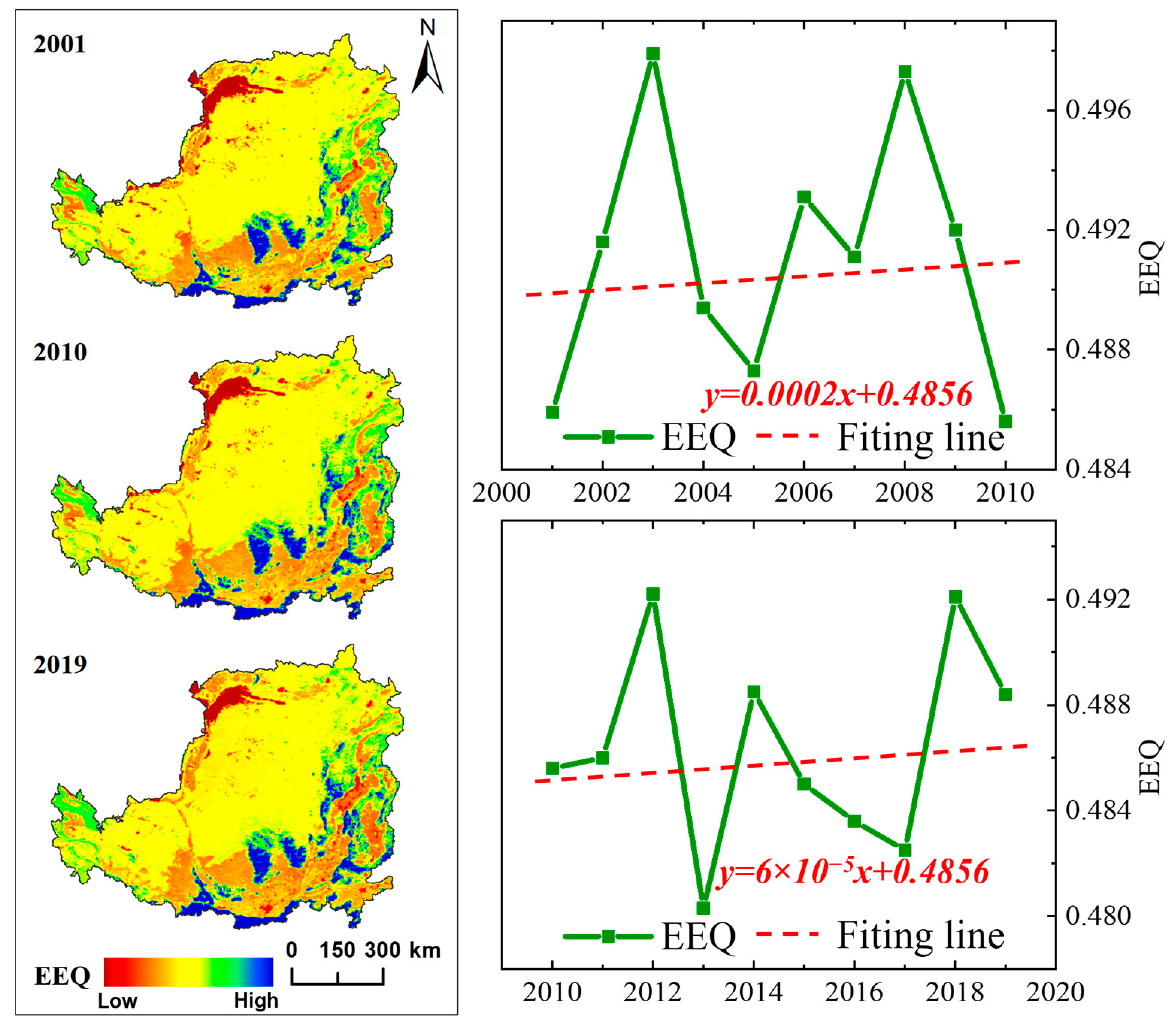
3.1. Temporal and Spatial Variation Characteristics of EEQ

The change in annual average EEQ in the LP during the study period is shown in Figure 3. In the time domain, the annual average EEQ of the LP showed a fluctuating upward trend from 2001 to 2010 (0.0002 a−1). The fluctuation of average EEQ from 2010 to 2019 is smaller than that from 2001 to 2010 (0.00005 a−1). In terms of spatial distribution, the EEQ of most LP is between 0.35 and 0.60 and relatively stable. It can be concluded from Figure 3 that the areas with low EEQ are mainly concentrated in Taiyuan and Linfen in Shanxi, Xian in Shaanxi, Lanzhou in Gansu, Xining in Qinghai, Yinchuan in Ningxia, and the Kubuqi Desert with its northwestern areas. The areas with EEQ above 0.50 were mainly distributed in the middle and lower reaches of the Yellow River Basin and the south of the LP. The areas with better ecological environments with an average EEQ higher than 0.6 are mainly distributed in the forest area of Yan’an and the Qinling Mountains in the south of Xi’an.

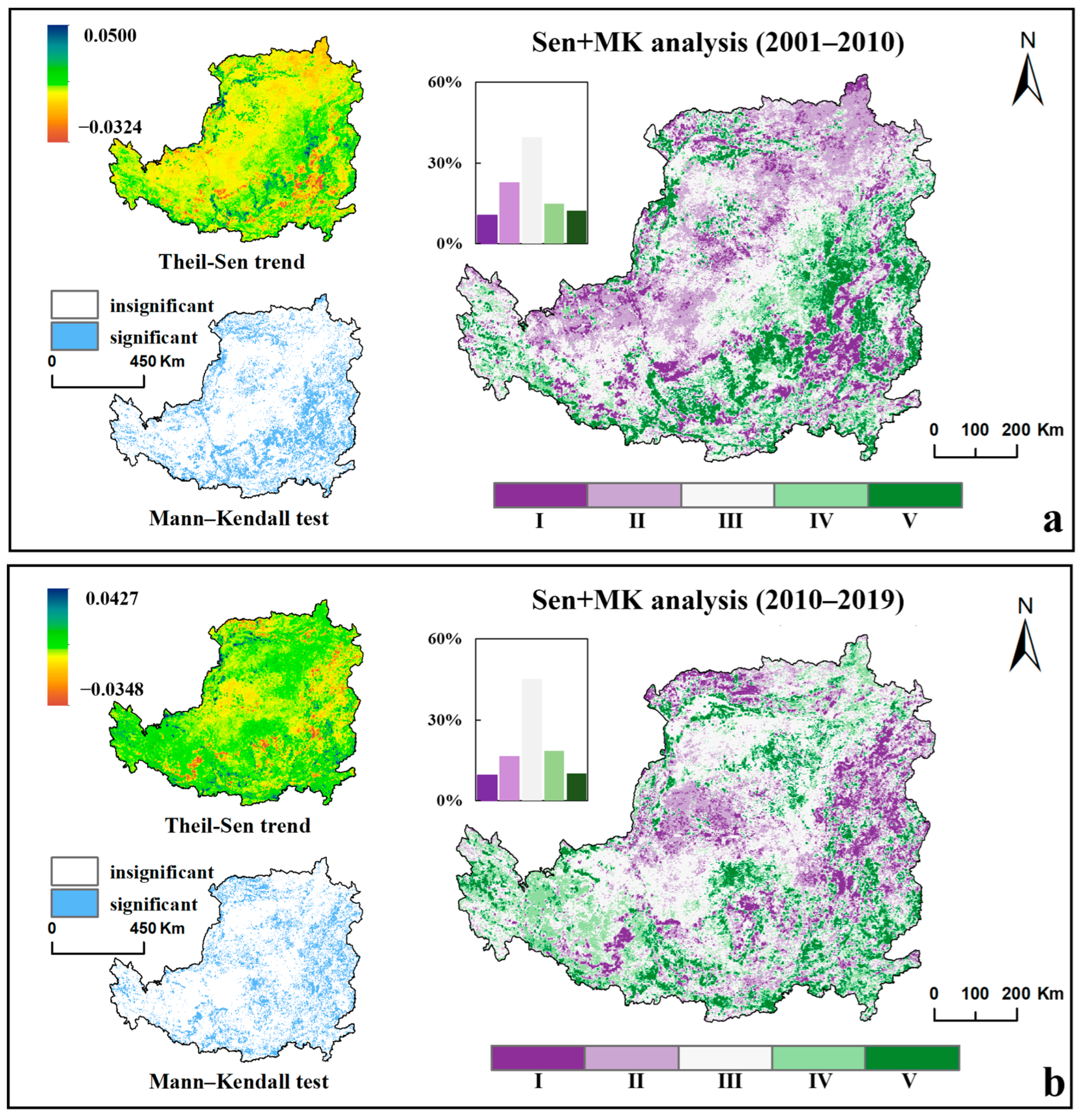
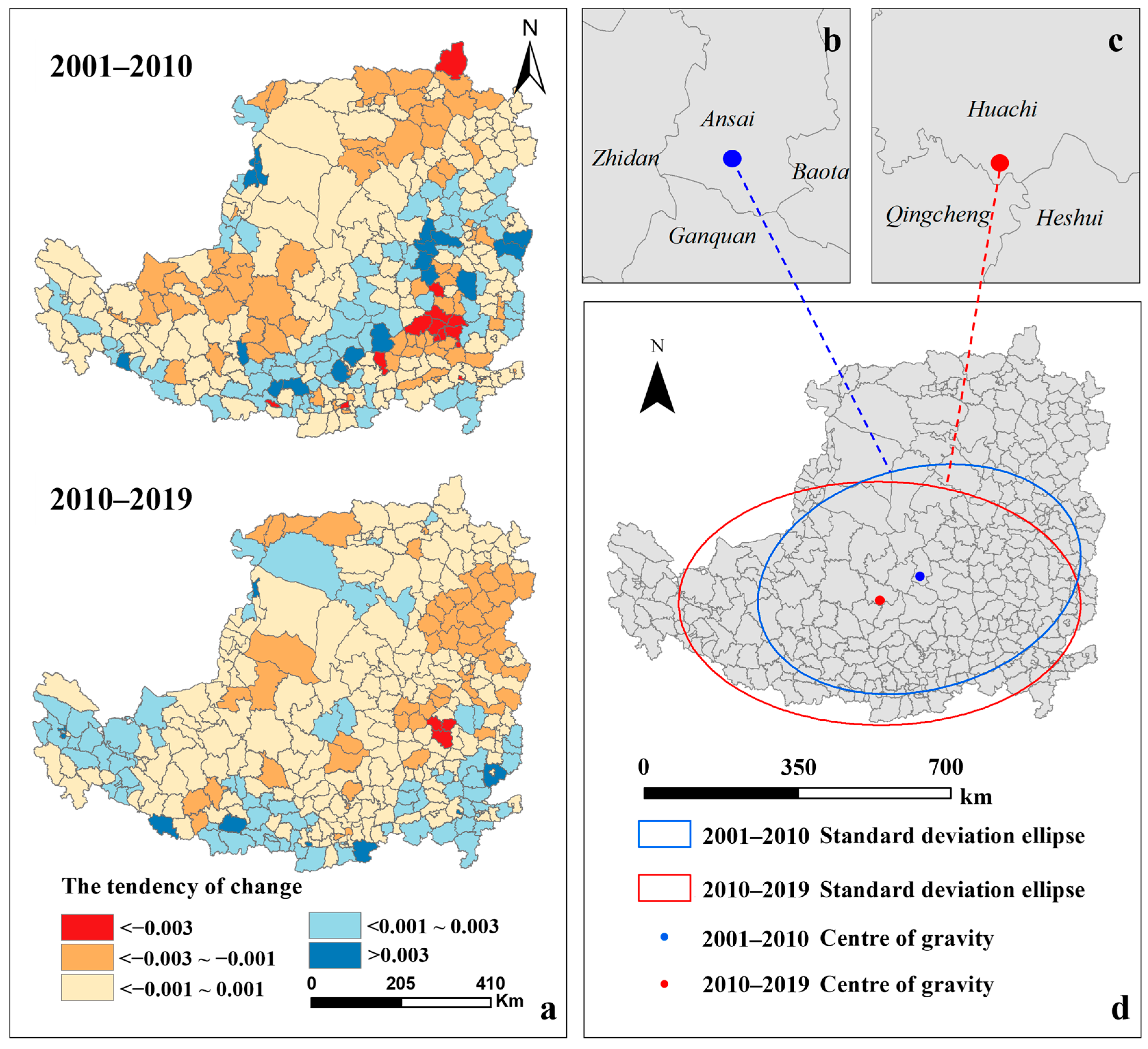
3.2. Evolution Trend Characteristics of EEQ

In order to further study the specific change trend of EEQ in the LP, the changes in EEQ during 2001–2010 and 2010–2019 were superimposed and analyzed (Figure 4). The evolution types were classified into five categories as shown in Table 3.
From 2001 to 2010 (Figure 4a), the areas with significant changes were mainly distributed in the central and southeastern regions of the LP. In the middle of the Taihang Mountain and the Lvliang Mountain, namely, the urban areas along the central and southern Shanxi Plateau (Taiyuan, Linfen, Yuncheng) showed a downward trend, while the EEQ around the urban area was significantly improved. At the same time, the EEQ in the northern part of Yan‘an and the northwestern part of Xi’an was also significantly improved. The EEQ in the south of Hohhot in the northwest of the LP, the northwest of the Shaanxi Plateau, and the Liupan Mountain area showed a downward trend. Through the pixel statistics of the change trend during this period (Table 3), it is known that significant degradation and slight degradation account for 33.38% of the total area, and the proportion of basically unchanged and above areas reaches 66.62%, of which the significantly improved area is 12.21%. The findings indicate that the EEQ was relatively stable in most areas of the LP during this period, while some areas showed a deteriorating trend.
From 2010 to 2019 (Figure 4b), the areas with significant changes shifted from the southeast to the central and eastern regions. Among them, the northeastern part of Shanxi (Taiyuan, Yuanping, Wutai Mountains) showed a significant downward trend as a whole. The area of Houtao in Hetao Plain, Mu Us Sandy Land in southern Ordos Plateau and Yan’an in Shaanxi Province also showed a downward trend. Gansu Longzhong Plateau and the mid-eastern Ordos Plateau have improved significantly compared with the past. It can be concluded that 26.09% of the area is degraded (Table 3), which is 21.84% lower than the previous period. The basically unchanged and above areas accounted for 73.91% of the total area, of which the basically unchanged area accounted for 45.25%, an increase of 14.30% compared with the past. The results show that the EEQ in this period has stabilized compared with the past.
As shown in Figure 5, the standard deviation ellipse contained most of the counties with high growth rates of EEQ. The long semi-axis of the standard deviation ellipse was 375.79 km during 2001–2010 and 459.64 km during 2010–2019, and the corresponding short semi-axis were 252.55 km and 277.48 km, respectively. The perimeter of the standard deviation ellipse increased from 1992.97 km in 2001–2010 to 2361.16 km in 2010–2019, indicating the expansion of the EEQ variation range. The increase in the long semi-axis and the decrease in the short semi-axis indicate that the growth rate of EEQ contracted significantly in the northeast direction and diffused significantly in the southwest direction. The center of gravity of the ellipse of the standard deviation of the growth rate of EEQ was distributed in Ansai County, Shaanxi Province during 2001–2010 (Figure 5b) and Huachi County, Gansu Province during 2010–2019 (Figure 5c), respectively, with a linear shift of 124.56 km to the southwest (Figure 5d).

3.3. Attribution Analysis of EEQ Spatial and Temporal Distribution

3.3.1. Regression Model Fitting Results

OLS analysis was performed on each dominant factor: precipitation (PRE), temperature (TEM), nighttime light (NL), land use index (LUI), and population (POP), and the results are shown in Table 4. OLS fitting results show that, from the analysis of the significance level of the overall parameters of each factor, the results are ideal. Each factor shows statistical significance, indicating that all dependent variables have no effect on the independent variable. The variance inflation factor test showed that the VIF values of each influencing factor were less than 7.5, indicating that there was no variable redundancy in the model, and there was no multiple linear relationship among the factors. In order to improve the goodness of fit, the GWR model needs to be introduced.
As it is necessary to compare the fitting results of GWR and MGWR, the data of independent variables (EEQ) and dependent variables (PRE, TEM, NL, LUI, POP) are standardized and imported into MGWR2.2, as developed by Oshan [60]. The centroid coordinates of each county after projection are inputted. The spatial kernel adopts the adaptive model, the bandwidth search method is the golden section method, the MGWR model type selects the Gaussian model, and the optimization criterion is AICc. From Table 5, the following can be revealed: In all three periods, the fit of MGWR was greater than that of the traditional GWR model, with MGWR’s AICc values in 2001, 2010, and 2019 being 21.1798, 9.5711, and 25.2128 lower than GWR, respectively, which is well above the threshold of 3 [63]. The bandwidth for the GWR model was set to 30 in 2001 and 2010, and then increased to 30 and 43 in 2019. However, the MGWR model revealed that different factors showed significant spatial heterogeneity over time. For instance, the PRE factor had a relatively large bandwidth of 103 in 2001, which accounted for 37.18% of the total bandwidth. This indicated that its impact on EEQ was extensive and less spatially diverse during that period. However, its bandwidth gradually decreased to 78 in 2010 and 47 in 2019, implying that its spatial heterogeneity became stronger, and EEQ became more sensitive to it. Finally, the proportion of the local regression standardized residual (SD) of the MGWR model in the range of [−2.5, 2.5] in all study years is more than 96% and shows that the model can meet the basic analysis.
In summary, based on the above model parameter determination, the results of the MGWR model in this study are better than the traditional model and with a certain feasibility. At the same time, MGWR quantifies the different bandwidths of the factors to characterize spatial heterogeneity and sensitivity. In ArcGIS 10.2, the regression coefficient of the MGWR model is spatially visualized to characterize the effect of each variable on the dependent variable in the local geographic space.

3.3.2. Results of MGWR-Based Regression Coefficients of Climate Factors

It can be seen from Figure 6a–c that PRE had a positive effect on the EEQ of the LP in most areas from 2001 to 2019. From the perspective of spatial relations, the impact of PRE gradually expanded from the mid-east towards the south and north. Regions with higher regression coefficients were mainly distributed in the south and have significantly expanded over time, indicating that the positive effect range of precipitation on EEQ in this region is gradually increasing. The regions with regression coefficients less than 0 are generally distributed in the mid-eastern regions of the LP (Yanan, Shaanxi Province and Linfen, Shanxi Province) and gradually shrink to the east over time, indicating that the negative effect range of precipitation in this region is gradually decreasing.
The variation of TEM and EEQ was illustrated in Figure 6d–f, showing a ‘two-way’ effect. From the perspective of spatial relationship, it mainly considers the strip area of the central LP (central Shanxi Province, northern Shaanxi Province) as the dividing line, and gradually changes to the north and south regions. The regions with a regression coefficient less than 0 are mainly distributed in the central and northern regions, and the regions with a regression coefficient less than 0.40 have expanded over time, extending to the eastern Ningxia and southern Inner Mongolia. The area with a regression coefficient greater than 0 is mainly distributed in the southwestern part of the LP (Lanzhou, Gansu Province) in 2001. Over time, it gradually shifts to the southeastern LP (Guanzhong Plain, eastern Henan Province).

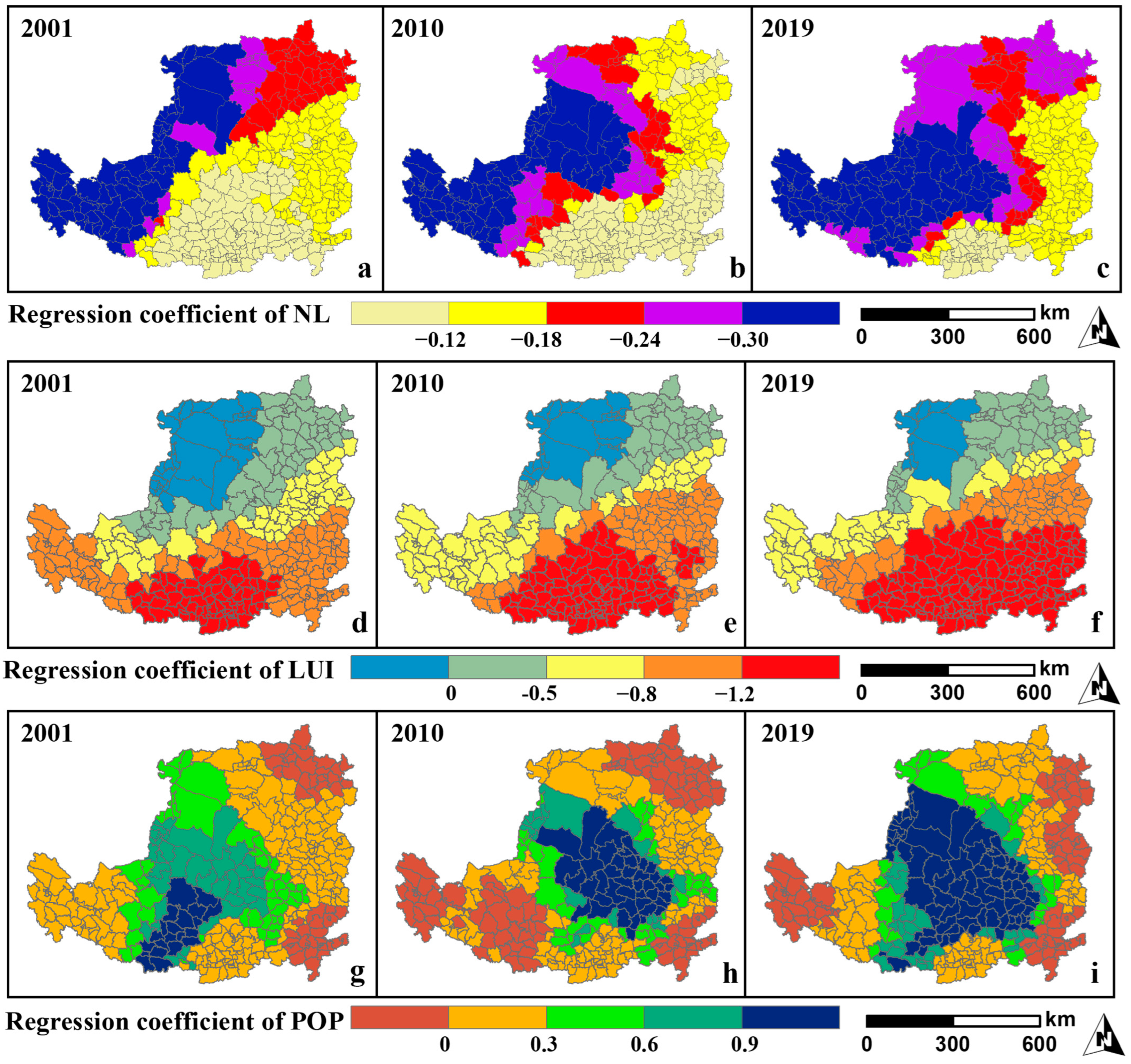
3.3.3. Results of MGWR-Based Regression Coefficients of Human Activities Factors

We used the regression spatial and temporal distribution of NL, LUI, and POP to characterize the impact of human activities on EEQ. The results are shown in Figure 7. It can be seen from Figure 7a–c that NL had a negative effect on EEQ mainly in 2001, especially in the southwestern region of the LP dominated by the eastern part of Qinghai Province and the northwestern desert region of the LP. Over time, the region with a regression coefficient less than—0.3 migrates and expands along the northwest to the southeast. For this part of the region, EEQ tends to decrease when NL is high, while the region with a regression coefficient greater than −0.08 expands from the south to the northeast from 2001 to 2019, and even some areas have positive values. It shows that the negative effects of NL in this part of these regions are significantly weakened.
The spatial and temporal distribution of EEQ and LUI regression are shown in Figure 7d–f. It is not difficult to see that except for the northwest of the LP (Erdos, Inner Mongolia), the regression coefficient is greater than 0, and most areas are less than 0, indicating that most areas have high land use intensity. The ecological environment is often poor, and the regression coefficient of LUI gradually increases from north to south. During the period from 2001 to 2019, the negative impact range of the southern region is expanding year by year, while the regions with positive regression coefficients in the northwest are decreasing year by year, indicating that the impact of land development on EEQ is increasing.
The spatial and temporal distribution of EEQ and POP regression are shown in Figure 7g–i. This shows that EEQ and POP are positively related in most of the central region. From 2001 to 2019, the regions with higher regression coefficients shifted and expanded from the southwest to the central region, and the population in these regions was often low when the EEQ value was low. At the same time, the regions with regression coefficients less than 0 showed the following characteristics: POP on EEQ in the southern (Luoyang-Sanmenxia, Henan Province) LP has been negative and almost constant in extent, while the northeastern one (Hohhot, Inner Mongolia-Datong, Shanxi) shifted to the southeast until the central of Shanxi Province. It is worth noting that there are also areas in the southwestern region (Xining, Qinghai Province) where POP has a negative effect on EEQ and cannot be underestimated.

4. Discussion

4.1. Temporal and Spatial Evolution of EEQ in the LP

From the temporal and spatial distribution and change trend of EEQ, the average ecological environment quality of the LP is between 0.48 and 0.50, and the overall average is general. In terms of the time dimension, the average value and its change rate during 2010–2019 are lower than that of 2001–2010. This suggests a decline in ecological environment quality over time [64,65]. This trend, along with the EEQ, suggests that vegetation coverage plays a significant role in the changes observed in EEQ. Regarding spatial distribution, the central and southern regions of the LP, particularly in Shaanxi, have displayed a notable improvement trend due to the implementation of several control measures and ecological construction projects. These findings align with the results reported by Dai et al. [66]. However, the northern and central parts of Shanxi have deteriorated. This is due to the serious ecological damage caused by mining development in the region, as mining activities will lead to a sinking of surface structures and geological calamity [67]. The results of the standard deviation ellipse show that although the growth rate of EEQ is slowing down, the growth area is expanding and there is a trend of migration to the southern region, indicating that the southern region is the focus of future changes in the LP. Using hot spot analysis for further verification (Figure 8), the results show that the high EEQ hot spot areas of LP are mainly distributed in the central regions of LP, and the cold spot areas are in Yinchuan, Ningxia, Xi’an, Shaanxi, and Luoyang, Henan, and other regions (Figure 8a). Over time, the hot spot area in the southeast (B1) has been expanding, and the changing rate in the mid-west area has slowed down (B2). The cold spot in the northwestern area (A1) has been reducing while the south area (A2) has been expanding (Figure 8b), shifting the center of gravity of EEQ growth to the southwest. To summarize, the analysis suggests a declining trend in ecological environment quality in the LP over time, with vegetation coverage playing a significant role in these changes. The implementation of control measures and ecological construction projects has led to improvements in certain regions, while mining development has caused deterioration in other areas. The southern region is projected to be the focus of future changes in EEQ.

4.2. Response of EEQ to Climate Change in the LP

LP is in a remote area of the continent with an arid climate. Scarce precipitation and large evaporation had caused a shortage of water resources and increasing sensitivity to climate change [68,69]. The results show the evolution process of the ecological environment of the LP on the regression coefficients of precipitation and temperature. The results of both analyses show that climatic factors play a positive role in the southern part of the LP and have gradually expanded over the past two decades. Compared with temperature, the positive effect of precipitation on the ecological environment is significantly greater, which is consistent with some research [70]. With the advancement of the ‘green map’ of the LP from north to south, sufficient precipitation becomes a necessary condition for vegetation growth in this area [71]. It is worth noting that the results of 2001 show that the increase in precipitation in the hilly and gully areas of the central LP will have a negative impact on the ecological environment. Since this period is in the early stage of the implementation of GGP, the regional vegetation restoration has not been effective. The region is one of the most serious areas of soil and water erosion in China [72]. Excessive rainstorms can cause soil erosion, which damages the ecological environment. Studies have shown that the frequency of rainstorms has increased in recent years [73]. Current research suggests that LST and NDBSI have a negative impact on the RSEI, while NDVI and WET have a positive impact [23,24,25,26,27,28]. GGP has been found to significantly improve NDVI [11,12,13,14,15,16,17,18,19,20,21,22,23,24,25,26,27,28,29,30,31,32,33,34,35], and a denser vegetation cover can help preserve soil and water, maintain a moist surface (WET), reduce LST, and regulate NDBSI and HQI. Therefore, GGP has a positive impact on the EEQ by changing LUCC.
With global climate warming and urbanization intensification [1], the average temperature of the Loess Plateau has also risen [74,75], and this climate change will have multiple impacts on vegetation growth and the ecological environment. On the one hand, it is generally believed that the growth of vegetation in the Northern Hemisphere is mainly limited by temperature [76], and climate warming is one of the main reasons for the improvement of vegetation productivity in the Northern Hemisphere over recent decades [77]. Therefore, an appropriate temperature increase in the southern regions with abundant rainfall is conducive to the growth of vegetation, improves NDVI, and thus increases EEQ. On the other hand, for northern regions, high temperatures and drought may lead to water loss, withering, or death of plant leaves, thus reducing NDVI and NPP. Higher temperatures also increase the rate at which water evaporates from the soil, preventing plants from making full use of water resources and further limiting their growth. In addition, it is worth noting that water resources are very important to the EEQ. With the rising temperature, the rainfall pattern and frequency in northern China may also change, resulting in the contradiction between the supply and demand of water resources [78]. High temperatures and drought will lead to lower soil moisture, and water shortage will seriously threaten the survival and growth of plants. In addition, insufficient water resources may lead to the degradation of the water ecosystem, resulting in the decrease in surface WET, the increase in LST, and the decrease in EEQ. Overall, attention should be given to the potential adverse effects of excessive precipitation in specific regions that are prone to soil and water erosion. The implementation of GGP has proven effective in improving vegetation cover and positively impacting EEQ through changes in NDVI, soil and water conservation, and regulation of surface temperature and built-up areas. Therefore, for the ecological environment of the northern region, the temperature change and the contradiction between the supply and demand of water resources are both important issues that need to be further studied and discussed.

4.3. Response of EEQ to Human Activities in the LP

The results show that among the three indexes of POP, NL, and LUI, the influence of LUI is the most significant, followed by POP and NL. The influence of LUI on EEQ decreased from south to north. This pattern could be attributed to the fact that the northern region is dominated by grassland and desert [8], with sparse vegetation and population density compared with the southeastern region [35]. Land development will destroy vegetation, reduce NDVI, and improve surface LST, but the impact of land development on EEQ will not be very significant under the harsh background environment. From 2001 to 2019, NL is mostly negative, which means that urbanization was less coupled with ecology in most regions. Some researchers have pointed out that the average coupling degree of new urbanization and ecological environment in the Yellow River Basin is in the range of 0.34–0.70 [79], and the coupling coordination degree shows a trend of increasing and then decreasing at the stage of confrontation and friction, which is similar to the trend of EEQ. The positive impact of POP in the LP center region has expanded significantly. POP and EEQ have a significant positive correlation in the central part of the LP and are negatively related in the surrounding and economically more-developed areas. On the one hand, this part of the region is a priority area for GGP promotion [80], but is less urbanized and economically developed than the southeastern region [81,82]. Even if the population grows naturally, this part of the region will improve ecologically with the advance of GGP. On the other hand, humans tend to build communities in places with better ecology, which means that the worse the EEQ in this part of the area, the less population. Additionally, it is worth noting that in some economically developed regions, the situation is the opposite and the demand for land development due to population growth in these areas can cause environmental degradation [83]. In terms of time scale, the urban areas of cities/counties on the Loess Plateau have grown exponentially over time [84]. Therefore, the critical issues lie in how to coordinate the development of urban areas around the LP with the ecological environment.

5. Conclusions

The ecological environment quality (EEQ) of the Loess Plateau (LP) generally is in the range of 0.48–0.50, with most regions falling within the general level. The south-central part of the LP has emerged as a hot spot for change, with a higher growth rate and average EEQ during 2001–2010 compared to 2010–2019. However, the proportion of regions with noticeable changes has decreased in the latter period, and the focus of ecological environment evolution has shifted towards the southern LP, with an expanded scope.
The MGWR model outperforms the GWR model in fitting EEQ with its driving factors. In terms of climate, the positive effects of precipitation and temperature on the ecological environment in the southern LP have become more prominent with the advancement of the Grain for Green Project (GGP), while the negative impact of temperature on the northwestern region is expanding. Human activities, such as land development intensity, have the greatest negative effect, which worsens from north to south. On the other hand, population growth in non-urban agglomeration areas, like the central LP, rarely has a detrimental impact on the ecological environment. Additionally, nighttime light has a more significant negative influence on the ecological environment in the western region than in the eastern region.
In conclusion, the implementation of the GGP over the past two decades has been effective in improving the EEQ of the LP. However, it is crucial to pay attention to maintaining the restoration effect in the central region, while also ensuring the reasonable development of land in the southern area. These findings highlight the need for ongoing efforts to preserve and improve the ecological environment of the LP.

Author Contributions

Conceptualization, X.Z.; Methodology, X.Z., G.S. and Y.C.; Validation, Y.C.; Formal analysis, Y.C., Y.L. (Yongcai Lou) and W.L.; Investigation, G.S., Y.L. (Yongcai Lou) and Y.Y.; Data curation, Y.L. (Yonghong Li); Writing—original draft, X.Z.; Writing—review & editing, Y.L. (Yongcai Lou) and W.L.; Visualization, Y.Y.; Supervision, Z.G.; Project administration, Z.G., Y.L. (Yonghong Li) and G.S.; Funding acquisition, Z.G. and Y.L. (Yonghong Li). All authors have read and agreed to the published version of the manuscript.

Funding

This research was funded by National Natural Science Foundation of China (Grant number 41671283).

Data Availability Statement

Not applicable.

Conflicts of Interest

The authors declare no conflict of interest.

References

  1. Hodson, R. Climate change. Nature 2017, 550, S53. [Google Scholar] [CrossRef]
  2. Lucas, R. The vulnerability of global forests to human and climate impacts. Nat. Sustain. 2023, 6, 354–355. [Google Scholar] [CrossRef]
  3. Liu, Y.; Liu, H.; Chen, Y.; Gang, C.; Shen, Y. Quantifying the contributions of climate change and human activities to vegetation dynamic in China based on multiple indices. Sci. Total Environ. 2022, 838, 156553. [Google Scholar] [CrossRef] [PubMed]
  4. IPCC. IPCC Fifth Assessment Report—Synthesis Report; IPPC: Rome, Italy, 2014. [Google Scholar]
  5. Li, Y.; Zhao, C.; Zhang, T.; Wang, W.; Duan, H.; Liu, Y.; Ren, Y.; Pu, Z. Impacts of Land-Use Data on the Simulation of Surface Air Temperature in Northwest China. J. Meteorol. Res. 2019, 32, 896–908. [Google Scholar] [CrossRef]
  6. Liu, J.; Kuang, W.; Zhang, Z.; Xu, X.; Qin, Y.; Ning, J.; Zhou, W.; Zhang, S.; Li, R.; Yan, C.; et al. Spatiotemporal characteristics, patterns, and causes of land-use changes in China since the late 1980s. J. Geogr. Sci. 2014, 24, 195–210. [Google Scholar] [CrossRef]
  7. Song, C.; Du, H.; Li, Y. Spatial and Temporal Variations in the Ecological Vulnerability of Northern China. J. Sens. 2022, 2022, 7232830. [Google Scholar] [CrossRef]
  8. Zhao, J.; Yang, Y.; Zhao, Q.; Zhao, Z. Effects of ecological restoration projects on changes in land cover: A case study on the Loess Plateau in China. Sci. Rep. 2017, 7, 44496. [Google Scholar] [CrossRef]
  9. Wang, Y.; Zhou, B.; Qin, D.; Wu, J.; Gao, R.; Song, L. Changes in mean and extreme temperature and precipitation over the arid region of northwestern China: Observation and projection. Adv. Atmos. Sci. 2017, 34, 289–305. [Google Scholar] [CrossRef]
  10. Ding, X.; Liu, X.; Liu, G.; Xiao, P.; Liu, R.; Gou, Z.; Zhao, Y. Comprehensive Assessment of Soil Conservation Measures by Rough Set Theory: A Case Study in the Yanhe River Basin of the Loess Plateau. Water 2022, 14, 2213. [Google Scholar] [CrossRef]
  11. Sun, W.; Song, X.; Mu, X.; Gao, P.; Wang, F.; Zhao, G. Spatiotemporal vegetation cover variations associated with climate change and ecological restoration in the Loess Plateau. Agric. For. Meteorol. 2015, 209–210, 87–99. [Google Scholar] [CrossRef]
  12. Zuo, S.; Dai, S.; Song, X.; Xu, C.; Liao, Y.; Chang, W.; Chen, Q.; Li, Y.; Tang, J.; Man, W. Determining the mechanisms that influence the surface temperature of urban forest canopies by combining remote sensing methods, ground observations, and spatial statistical models. Remote Sens. 2018, 10, 1814. [Google Scholar] [CrossRef]
  13. Liu, L.; Zhang, H.; Zhang, Y.; Li, F.; Chen, X.; Wang, Y.; Wang, Y. Spatiotemporal heterogeneity correction in land ecosystem services and its value assessment: A case study of the Loess Plateau of China. Environ. Sci. Pollut. Res. Int. 2023, 30, 47561–47579. [Google Scholar] [CrossRef] [PubMed]
  14. Cen, Y.; Lou, Y.; Gao, Z.; Liu, W.; Zhang, X.; Sun, G.; Li, Y. Vegetation carbon input moderates the effects of climate change on topsoil organic carbon in China. Catena 2023, 228, 107188. [Google Scholar] [CrossRef]
  15. Jing, P.; Zhang, D.; Ai, Z.; Wu, H.; Zhang, D.; Ren, H.; Suo, L. Responses of Ecosystem Services to Climate Change: A Case Study of the Loess Plateau. Forests 2022, 13, 2011. [Google Scholar] [CrossRef]
  16. Qu, Z.; Zhao, Y.; Luo, M.; Han, L.; Yang, S.; Zhang, L. The Effect of the Human Footprint and Climate Change on Landscape Ecological Risks: A Case Study of the Loess Plateau, China. Land 2022, 11, 217. [Google Scholar] [CrossRef]
  17. Zhang, B.; Tian, L.; Zhao, X.; Wu, P. Feedbacks between vegetation restoration and local precipitation over the Loess Plateau in China. Sci. China Earth Sci. 2021, 64, 920–931. [Google Scholar] [CrossRef]
  18. Luo, W.; Bai, H.; Jing, Q.; Liu, T.; Xu, H. Urbanization-induced ecological degradation in Midwestern China: An analysis based on an improved ecological footprint model. Resour. Conserv. Recycl. 2018, 137, 113–125. [Google Scholar] [CrossRef]
  19. Lu, C.; Liu, W.; Huang, P.; Wang, Y.; Tang, X. Effect of Energy Utilization and Economic Growth on the Ecological Environment in the Yellow River Basin. Int. J. Environ. Res. Public Health 2023, 20, 2345. [Google Scholar] [CrossRef]
  20. Lei, P.; Zhang, H.; Wu, Q.; Li, P.; Wang, B.; Wu, P. The Development of Environmental Geoscience Contributes to the Construction of Ecological Civilization. Bull. Environ. Contam. Toxicol. 2022, 109, 659–660. [Google Scholar] [CrossRef]
  21. Liu, Y.; Dang, C.; Yue, H.; Lyu, C.; Jiaxin, Q.; Zhu, R. Comparison between Modified Remote Sensing Ecological Index and RSEI. J. Remote Sens. 2022, 26, 683–697. [Google Scholar] [CrossRef]
  22. Xu, H. A remote sensing urban ecological index. Acta Ecol. Sin. 2013, 33, 7853–7862. [Google Scholar]
  23. Zhou, J.; Liu, W. Monitoring and Evaluation of Eco-Environment Quality Based on Remote Sensing-Based Ecological Index (RSEI) in Taihu Lake Basin, China. Sustainability 2022, 14, 5642. [Google Scholar] [CrossRef]
  24. Liu, X.; Zhang, X.; He, Y.; Luan, H. Monitoring and assessment of ecological change in coastal cities based on RSEI. ISPRS-Int. Arch. Photogramm. Remote Sens. Spat. Inf. Sci. 2020, 42, 461–470. [Google Scholar] [CrossRef]
  25. Yuan, B.; Fu, L.; Zou, Y.; Zhang, S.; Chen, X.; Li, F.; Deng, Z.; Xie, Y. Spatiotemporal change detection of ecological quality and the associated affecting factors in Dongting Lake Basin, based on RSEI. J. Clean. Prod. 2021, 302, 126995. [Google Scholar] [CrossRef]
  26. Gong, E.; Shi, F.; Wang, Z.; Hu, Q.; Zhang, J.; Hai, H. Evaluating Environmental Quality and Its Driving Force in Northeastern China Using the Remote Sensing Ecological Index. Sustainability 2022, 14, 16304. [Google Scholar] [CrossRef]
  27. Zhang, J.; Zhou, Q.; Cao, M.; Liu, H. Spatiotemporal Change of Eco-Environmental Quality in the Oasis City and Its Correlation with Urbanization Based on RSEI: A Case Study of Urumqi, China. Sustainability 2022, 14, 9227. [Google Scholar] [CrossRef]
  28. Xiong, Y.; Xu, W.; Lu, N.; Huang, S.; Wu, C.; Wang, L.; Dai, F.; Kou, W. Assessment of spatial–temporal changes of ecological environment quality based on RSEI and GEE: A case study in Erhai Lake Basin, Yunnan province, China. Ecol. Indic. 2021, 125, 107518. [Google Scholar] [CrossRef]
  29. Yang, W.; Zhou, Y.; Li, C. Assessment of Ecological Environment Quality in Rare Earth Mining Areas Based on Improved RSEI. Sustainability 2023, 15, 2964. [Google Scholar] [CrossRef]
  30. Wang, J.; Li, G.; Chen, F. Eco-Environmental Effect Evaluation of Tamarix chinesis Forest on Coastal Saline-Alkali Land Based on RSEI Model. Sensors 2022, 22, 5052. [Google Scholar] [CrossRef]
  31. Zongfan, B.; Ling, H.; Huiqun, L.; Xuhai, J.; Liangzhi, L. Spatiotemporal change and driving factors of ecological status in Inner Mongolia based on the modified remote sensing ecological index. Environ. Sci. Pollut. Res. Int. 2023, 30, 52593–52608. [Google Scholar] [CrossRef]
  32. Jia, H.; Yan, C.; Xing, X. Evaluation of Eco-Environmental Quality in Qaidam Basin Based on the Ecological Index (MRSEI) and GEE. Remote Sens. 2021, 13, 4543. [Google Scholar] [CrossRef]
  33. Xu, D.; Yang, F.; Yu, L.; Zhou, Y.; Li, H.; Ma, J.; Huang, J.; Wei, J.; Xu, Y.; Zhang, C.; et al. Quantization of the coupling mechanism between eco-environmental quality and urbanization from multisource remote sensing data. J. Clean. Prod. 2021, 321, 128948. [Google Scholar] [CrossRef]
  34. Jing, G.; Dong, X.; Yuhao, W.; Jia, G.; Bingnan, R.; Feng, Y. Spatio-temporal evolution of eco-environment quality and the response to climate change and human activities in Hainan Island. Acta Ecol. Sin. 2022, 42, 4795–4806. [Google Scholar]
  35. He, P.; Xu, L.; Liu, Z.; Jing, Y.; Zhu, W. Dynamics of NDVI and its influencing factors in the Chinese Loess Plateau during 2002–2018. Reg. Sustain. 2021, 2, 36–46. [Google Scholar] [CrossRef]
  36. Chen, S.; Zhang, Q.; Chen, Y.; Zhou, H.; Xiang, Y.; Liu, Z.; Hou, Y. Vegetation Change and Eco-Environmental Quality Evaluation in the Loess Plateau of China from 2000 to 2020. Remote Sens. 2023, 15, 424. [Google Scholar] [CrossRef]
  37. Sun, C.; Li, X.; Zhang, W.; Li, X. Evolution of Ecological Security in the Tableland Region of the Chinese Loess Plateau Using a Remote-Sensing-Based Index. Sustainability 2020, 12, 3489. [Google Scholar] [CrossRef]
  38. Hao, Y.; Liu, Y.-M. The influential factors of urban PM2. 5 concentrations in China: A spatial econometric analysis. J. Clean. Prod. 2016, 112, 1443–1453. [Google Scholar] [CrossRef]
  39. He, Y.; Yi, G.; Zhang, T. The EVI trends and driving factors in Red River Basin affected by the “corridor-corridorbarrier” function during 2000–2014. ACTA Ecol. Sin. 2018, 38, 2056–2064. [Google Scholar]
  40. Wang, J.; Xu, C. Geodetector: Principle and prospective. Acta Geogr. Sin. 2017, 72, 116–134. [Google Scholar] [CrossRef]
  41. Geng, J.; Yu, K.; Xie, Z.; Zhao, G.; Ai, J.; Yang, L.; Yang, H.; Liu, J. Analysis of Spatiotemporal Variation and Drivers of Ecological Quality in Fuzhou Based on RSEI. Remote Sens. 2022, 14, 4900. [Google Scholar] [CrossRef]
  42. Fotheringham, A.S.; Yang, W.; Kang, W. Multiscale Geographically Weighted Regression (MGWR). Ann. Am. Assoc. Geogr. 2017, 107, 1247–1265. [Google Scholar] [CrossRef]
  43. Yang, Y.; Li, H. Monitoring spatiotemporal characteristics of land-use carbon emissions and their driving mechanisms in the Yellow River Delta: A grid-scale analysis. Environ. Res. 2022, 214, 114151. [Google Scholar] [CrossRef]
  44. Zhou, M.-G.; Yang, Y.; Sun, Y.; Zhang, F.-Y.; Li, Y.-H. Spatio-temporal characteristics of air quality and influencing factors in Shandong Province from 2016 to 2020. Huanjing Kexue 2022, 43, 2937–2946. [Google Scholar] [PubMed]
  45. Wang, Y.; Fu, B.; Chen, L.; Lü, Y.; Gao, Y. Check dam in the Loess Plateau of China: Engineering for environmental services and food security. Environ. Sci. Technol. 2011, 45, 10298–10299. [Google Scholar] [CrossRef]
  46. Zheng, K.; Wei, J.Z.; Pei, J.Y.; Cheng, H.; Zhang, X.L.; Huang, F.Q.; Li, F.M.; Ye, J.S. Impacts of climate change and human activities on grassland vegetation variation in the Chinese Loess Plateau. Sci. Total Environ. 2019, 660, 236–244. [Google Scholar] [CrossRef] [PubMed]
  47. Chen, L.; Wei, W.; Fu, B.; Lü, Y. Soil and water conservation on the Loess Plateau in China: Review and perspective. Prog. Phys. Geogr. Earth Environ. 2016, 31, 389–403. [Google Scholar] [CrossRef]
  48. Yang, J.; Huang, X. The 30 m annual land cover dataset and its dynamics in China from 1990 to 2019. Earth Syst. Sci. Data 2021, 13, 3907–3925. [Google Scholar] [CrossRef]
  49. Lixian, Z.; Zhehao, R.; Bin, C.; Peng, G.; Haohuan, F.; Bing, X. A Prolonged Artificial Nighttime-Light Dataset of China (1984–2020); National Tibetan Plateau Data Center: Beijing, China, 2021. [Google Scholar] [CrossRef]
  50. Theil, H. A Rank-Invariant Method of Linear and Polynomial Regression Analysis. In Henri Theil’s Contributions to Economics and Econometrics: Econometric Theory and Methodology; Raj, B., Koerts, J., Eds.; Springer: Dordrecht, The Netherlands, 1992; pp. 345–381. [Google Scholar]
  51. Mann, H.B. Nonparametric tests against trend. Econom. J. Econom. Soc. 1945, 245–259. [Google Scholar] [CrossRef]
  52. Kendall, M.G. Rank Correlation Methods. Br. J. Psychol. 1990, 25, 86–91. [Google Scholar] [CrossRef]
  53. Verburg, P.H.; Crossman, N.; Ellis, E.C.; Heinimann, A.; Hostert, P.; Mertz, O.; Nagendra, H.; Sikor, T.; Erb, K.-H.; Golubiewski, N.; et al. Land system science and sustainable development of the earth system: A global land project perspective. Anthropocene 2015, 12, 29–41. [Google Scholar] [CrossRef]
  54. Feng, H.; Wang, S.; Zou, B.; Nie, Y.; Ye, S.; Ding, Y.; Zhu, S. Land use and cover change (LUCC) impacts on Earth’s eco-environments: Research progress and prospects. Adv. Space Res. 2023, 71, 1418–1435. [Google Scholar] [CrossRef]
  55. Liu, Z.a. Study on The Model of Regional Differentiation of Land Use Degree in China. J. Nat. Resour. 1997, 12, 105–111. [Google Scholar] [CrossRef]
  56. Lefever, D.W. Measuring geographic concentration by means of the standard deviational ellipse. Am. J. Sociol. 1926, 32, 88–94. [Google Scholar] [CrossRef]
  57. Dempster, A.P.; Schatzoff, M.; Wermuth, N. A simulation study of alternatives to ordinary least squares. J. Am. Stat. Assoc. 1977, 72, 77–91. [Google Scholar] [CrossRef]
  58. Fotheringham, A.; Brunsdon, C.; Charlton, M. Geographically Weighted Regression: The Analysis of Spatially Varying Relationships; John Wiley & Sons: Hoboken, NJ, USA, 2002; p. 13. [Google Scholar]
  59. Yu, H.; Fotheringham, A.S.; Li, Z.; Oshan, T.; Kang, W.; Wolf, L.J. Inference in Multiscale Geographically Weighted Regression. Geogr. Anal. 2019, 52, 87–106. [Google Scholar] [CrossRef]
  60. Oshan, T.; Li, Z.; Kang, W.; Wolf, L.; Fotheringham, A. mgwr: A Python Implementation of Multiscale Geographically Weighted Regression for Investigating Process Spatial Heterogeneity and Scale. ISPRS Int. J. Geo-Inf. 2019, 8, 269. [Google Scholar] [CrossRef]
  61. Liu, X.; Zhang, C.; Yu, T.; Ji, W.; Wu, T.; Zhuo, X.; Li, C.; Li, B.; Wang, L.; Shao, Y.; et al. Identification of the spatial patterns and controlling factors of Se in soil and rice in Guangxi through hot spot analysis. Environ. Geochem. Health 2023, 45, 4477–4492. [Google Scholar] [CrossRef]
  62. Getis, A.; Ord, J.K. The Analysis of Spatial Association by Use of Distance Statistics. In Perspectives on Spatial Data Analysis; Anselin, L., Rey, S.J., Eds.; Springer: Berlin/Heidelberg, Germany, 2010; pp. 127–145. [Google Scholar]
  63. Brunsdon, C.; Fotheringham, S.; Charlton, M. Geographically Weighted Regression. J. R. Stat. Soc. Ser. D 1998, 47, 431–443. [Google Scholar] [CrossRef]
  64. Ting, L.; Lü, Y.; Ren, Y.; Li, P. Gauging the effectiveness of vegetation restoration and the influence factors in the Loess Plateau. Acta Ecol. Sin. 2020, 40, 8593–8605. [Google Scholar]
  65. Zhang, Y.; Jiang, X.; Lei, Y.; Gao, S. The contributions of natural and anthropogenic factors to NDVI variations on the Loess Plateau in China during 2000–2020. Ecol. Indic. 2022, 143, 109342. [Google Scholar] [CrossRef]
  66. Dai, Q.; Cui, C.F.; Wang, S. Spatiotemporal variation and sustainability of NDVI in the Yellow River basin. Irrig. Drain. 2022, 71, 1304–1318. [Google Scholar] [CrossRef]
  67. Balat, M. Influence of Coal as an Energy Source on Environmental Pollution. Energy Sources 2007, 29, 581–589. [Google Scholar] [CrossRef]
  68. Zhang, B.; He, C.; Burnham, M.; Zhang, L. Evaluating the coupling effects of climate aridity and vegetation restoration on soil erosion over the Loess Plateau in China. Sci. Total Environ. 2016, 539, 436–449. [Google Scholar] [CrossRef] [PubMed]
  69. Zhao, X.; Wu, P.; Gao, X.; Persaud, N. Soil quality indicators in relation to land use and topography in a small catchment on the Loess Plateau of China. Land Degrad. Dev. 2015, 26, 54–61. [Google Scholar] [CrossRef]
  70. Chen, Y.; Jiao, J.; Tian, H.; Xu, Q.; Feng, X.; Wang, N.; Bai, L.; Yang, X. Spatial correlation analysis between vegetation NDVI and natural environmental factors based on geographical detector on the Loess Plateau. Acta Ecol. Sin. 2022, 42, 3569–3580. [Google Scholar]
  71. Cen, Y.; Gao, Z.; Sun, G.; Lou, Y.; Zhang, S.; Li, Y.; Wu, T. Effects of soil conservation on the spatial heterogeneity of vegetation carbon sequestration in the Yellow River Basin, China. Land Degrad. Dev. 2023, 34, 4607–4622. [Google Scholar] [CrossRef]
  72. Gong, L.; Jin, C.; Sun, W.; Yang, H.; Wang, J. Loess plateau rainfalls characteristics and influences on soil erosion. J. Food Agric. Environ. 2013, 11, 2502–2505. [Google Scholar]
  73. Donat, M.G.; Lowry, A.L.; Alexander, L.V.; O’Gorman, P.A.; Maher, N. More extreme precipitation in the world’s dry and wet regions. Nat. Clim. Chang. 2016, 6, 508–513. [Google Scholar] [CrossRef]
  74. Fu, B.; Liu, Y.; Lü, Y.; He, C.; Zeng, Y.; Wu, B. Assessing the soil erosion control service of ecosystems change in the Loess Plateau of China. Ecol. Complex. 2011, 8, 284–293. [Google Scholar] [CrossRef]
  75. Woodward, A.; Smith, K.R.; Campbell-Lendrum, D.; Chadee, D.D.; Honda, Y.; Liu, Q.; Olwoch, J.; Revich, B.; Sauerborn, R.; Chafe, Z.; et al. Climate change and health: On the latest IPCC report. Lancet 2014, 383, 1185–1189. [Google Scholar] [CrossRef]
  76. Chen, C.; He, B.; Guo, L.; Zhang, Y.; Xie, X.; Chen, Z. Identifying critical climate periods for vegetation growth in the Northern Hemisphere. J. Geophys. Res. Biogeosci. 2018, 123, 2541–2552. [Google Scholar] [CrossRef]
  77. Zhang, Y.; Piao, S.; Sun, Y.; Rogers, B.M.; Li, X.; Lian, X.; Liu, Z.; Chen, A.; Peñuelas, J. Future reversal of warming-enhanced vegetation productivity in the Northern Hemisphere. Nat. Clim. Chang. 2022, 12, 581–586. [Google Scholar] [CrossRef]
  78. Sun, W.; Mu, X.; Song, X.; Wu, D.; Cheng, A.; Qiu, B. Changes in extreme temperature and precipitation events in the Loess Plateau (China) during 1960–2013 under global warming. Atmos. Res. 2016, 168, 33–48. [Google Scholar] [CrossRef]
  79. Jianji, Z.; Yan, L.; Yakun, Z.; Shengli, Q.; Yanhua, W.; Changhong, M. Spatiotemporal differentiation and influencing factors of the coupling and coordinated development of new urbanization and ecological environment in the Yellow River Basin. Resour. Sci. 2020, 42, 159–171. [Google Scholar]
  80. Wang, J.; Liu, Z.; Gao, J.; Emanuele, L.; Ren, Y.; Shao, M.; Wei, X. The Grain for Green project eliminated the effect of soil erosion on organic carbon on China’s Loess Plateau between 1980 and 2008. Agric. Ecosyst. Environ. 2021, 322, 107636. [Google Scholar] [CrossRef]
  81. Xiang, K.; Zhao, A.; Liu, H.; Zhang, X.; Zhang, A.; Tian, X.; Jin, Z. Spatiotemporal Evolution and Coupling Pattern Analysis of Urbanization and Ecological Environmental Quality of the Chinese Loess Plateau. Sustainability 2022, 14. [Google Scholar] [CrossRef]
  82. Song, Y.-Y.; Ma, B.-B.; Dai, L.-H.; Xue, D.-Q.; Xia, S.-Y.; Wang, P.-T. Spatial-temporal pattern and formation mechanism of county urbanization on the Chinese Loess Plateau. J. Mt. Sci. 2021, 18, 1093–1111. [Google Scholar] [CrossRef]
  83. Seto, K.C.; Fragkias, M.; Güneralp, B.; Reilly, M.K. A meta-analysis of global urban land expansion. PLoS ONE 2011, 6, e23777. [Google Scholar] [CrossRef]
  84. Chen, W.; Xu, Q.; Zhao, K.; Hao, L.; Pu, C.; Yuan, S. Spatiotemporal expansion modes of urban areas on the Loess Plateau from 1992 to 2021 based on nighttime light images. Int. J. Appl. Earth Obs. Geoinf. 2023, 118, 103262. [Google Scholar] [CrossRef]
Figure 1. Topography and geographical location of the LP (a,b), land use of the LP in 2010 (c), the average annual precipitation and temperature of the LP during 2001–2019 (d).
Land 12 01792 g001
Figure 2. The technology roadmap for this study.
Land 12 01792 g002
Figure 3. Temporal and spatial distribution of EEQ in LP from 2001 to 2019.
Land 12 01792 g003
Figure 4. Spatial distribution of evolutionary trends in ecological quality from 2001 to 2010 (a), spatial distribution of evolutionary trends in ecological quality from 2010 to 2019 (b).
Land 12 01792 g004
Figure 5. Trends in EEQ evolution based on LP county scale (a), the center of gravity of EEQ changes from 2001 to 2010 (b), the center of gravity of EEQ changes from 2010 to 2019 (c), the elliptical spatial distribution of standard deviation of EEQ changes from 2001 to 2019 (d).
Land 12 01792 g005
Figure 6. Spatial and temporal distribution of regression coefficients of precipitation (ac), spatial and temporal distribution of regression coefficients of temperature (df).
Land 12 01792 g006
Figure 7. Spatial and temporal distribution of regression coefficients of nighttime light (ac), spatial and temporal distribution of regression coefficients of land use index (df), spatial and temporal distribution of regression coefficients of population (gi).
Land 12 01792 g007
Figure 8. Spatial and temporal trends of cold and hot spots in the LP (a); remote sensing images of typical feature areas (b) and Landsat satellite remote sensing images read by Google Earth.
Land 12 01792 g008
Table 1. Detailed description of data sources.
Data NameSpatial ResolutionTime ResolutionTime RangeSource
LANDSAT/LT05/C02/T1_L2
LANDSAT/LC08/C02/T1_L2
30 m16-day2001–2019 USGS a
Annual land cover data of China (CLCD)30 mYear2001, 2010, 2019 Paper [48]
(https://zenodo.org/record/5816591 (accessed on 25 May 2022))
Nighttime light Dataset of China (NL)1 kmYear2001, 2010, 2019Paper [49]
(https://data.tpdc.ac.cn (accessed on 3 March 2023))
Population density dataset
(POP)
1 kmYear2001, 2010, 2019LandScan b
Precipitation data
(PRE)
1 kmMonth2001–2019 ESSDC c
Temperature data
(TEM)
1 kmMonth2001–2019 ESSDC d
Digital elevation model
(DEM)
30 mN/AN/ARESDC d
China’s provincial boundaries, river networksN/AN/A2015 RESDC d
a: United States Geological Survey (www.earthexplorer.usgs.gov (accessed on 16 March 2023)). b: LandScan USA (www.landscan.ornl.gov (accessed on 16 March 2023)). c: Earth System Science Data Center China (www.loess.geodata.cn (accessed on 25 May 2022)). d: Recourses and Environment Science Data Center China (www.resdc.cn (accessed on 25 May 2022)).
Table 2. Ingredient calculation formula.
IndicatorsCalculation Formula
NDVINDVI = (ρNIR − ρred)/(ρNIR + ρred)
WETWETTM = 0.0315ρblue + 0.2021ρgreen + 0.3102ρred + 0.1594ρNIR − 0.6806ρSWIR1 − 0.6109ρSWIR2
WETOLI = 0.1511ρblue + 0.1973ρgreen + 0.3283ρred + 0.3407ρNIR − 0.7117ρSWIR1 − 0.4559ρSWIR2
NDBSINDBSI = (SI+IBI)/2
IBI = IBI1/IBI2
IBI1 = 2ρSWIR2/(ρSWIR1 + ρNIR) − [(ρNIR/(ρred + ρNIR)+ρgreen/(ρSWIR1 + ρgreen)]
IBI2 = 2ρSWIR2/(ρSWIR1 + ρNIR) + [(ρNIR/(ρred + ρNIR)+ρgreen/(ρSWIR1 + ρgreen)]
SI = [(ρSWIR1 + ρred) − (ρblue + ρNIR)]/[(ρSWIR1 + ρred)+(ρblue + ρNIR)]
LSTLST = T/[1 + (λT/ρ)lnε] − 273.15
HQIHQI = μ × (0.35 × Forest + 0.21 × Grassland + 0.28 × Water + 0.11 × Cropland + 0.04 × Impervious + 0.01 × Barren)/Area
ρblue, ρgreen, ρred, ρNIR, ρSWIR1, ρSWIR2: represent the reflectance of Landsat 5 TM and Landsat 8 OLI in blue, green, red, near-infrared, shortwave infrared 1, and shortwave infrared 2, respectively; T: heat value of the sensor; λ: center wavelength of the thermal infrared band; ρ: constant; ε: specific surface emissivity.
Table 3. Pixel statistics of ecological environment quality change trend.
Theil−Sen SlopeZ ValueType of Change2001–2010 2010–2019
Area/km2PercentageArea/km2Percentage
<−0.001<−1.96I68,28810.52%61,7549.52%
<−0.001−1.96~1.96II148,33822.86%107,56016.57%
−0.001~0.001−1.96~1.96III256,92139.59%293,66345.25%
>0.001−1.96~1.96IV96,22514.83%120,19618.52%
>0.001>1.96V79,24212.21%65,84110.14%
Table 4. OLS model estimation and diagnosis results.
YearVariableRobust PVIFAdjust R2
2001Intercept0.0000 ***--------0.4630
PRE0.0000 ***1.3399
TEM0.0514 *1.7830
NL0.0191 **6.6650
LUI0.0001 ***2.4521
POP0.0122 **5.5689
2010Intercept0.0000 ***--------0.5911
PRE0.0021 ***3.9585
TEM0.0000 ***1.5539
NL0.0414 **1.9673
LUI0.0000 ***2.9405
POP0.20182.8629
2019Intercept0.0000 ***--------0.5815
PRE0.0018 ***3.1993
TEM0.0000 ***1.2082
NL0.03950 **1.8455
LUI0.0000 ***3.0620
POP0.0663 *2.2359
*: significant at 0.1 level, **: significant at 0.05 level, ***: significant at 0.01 level.
Table 5. The results of GWR and MGWR.
YearVariableGWRMGWR
BandAICcAdjust R2BandAICcAdjust R2SD ∈ |2.5|
2001intercept30424.26690.837930403.08710.840396.1876%
PRE30103
TEM3030
NL3043
LUI3030
POP3041
2010intercept30372.08220.875030362.51110.892097.9474%
PRE3078
TEM3030
NL3047
LUI3034
POP3030
2019intercept43377.73870.851230352.52590.859098.2405%
PRE4347
TEM4330
NL4330
LUI4332
POP4331
Disclaimer/Publisher’s Note: The statements, opinions and data contained in all publications are solely those of the individual author(s) and contributor(s) and not of MDPI and/or the editor(s). MDPI and/or the editor(s) disclaim responsibility for any injury to people or property resulting from any ideas, methods, instructions or products referred to in the content.

