Abstract
Current digital soil mapping of soil properties (soil organic carbon, SOC; electrical conductivity, EC; and pH) is mainly based on transfer learning, which is inadequate in terms of accuracy for the northern plain area of Xinjiang. To address this issue, establishing a new model is urgently required that can improve our understanding of the soil properties in this region. To this end, based on the global bioclimatic variables and surface dry–wet and wet–dry transitions, The study developed a spectral–water–heat database (SWHD). The study then incorporated this database and background data into machine learning algorithms (XGBoost, LightGBM, and random forest) to establish models applicable to the study area and draw spatial changes in the key soil properties. Our findings revealed that the organic carbon content was the highest in grasslands, whereas shrublands had high soil salinity. The pH value indicated overall alkalinity in the study area. Additionally, the SWHD-based predictions outperformed the mean or maximum value datasets, with LightGBM showing superior performance among all models. Furthermore, the validation accuracy obtained through our optimal algorithm was significantly higher than that obtained by other products, such as Harmonized World Soil Database (HWSD) and SoilGrid250, likely because of the limitations of these datasets, which may represent historical soil properties rather than current variations in the soil properties in the region. The study also observed that the mean SOC and EC values significantly decreased compared to the historical data, while the decrease in pH was smaller but not significant. Structural equation modeling and variable importance analysis revealed that the variables with the greatest influence on modeling SOC, EC, and pH were BIO10, DTW2021_406-426_B3 (Surface reflectance acquired in spring), and land use type. Our improved model developed based on the SWHD dataset offers important scientific evidence and decision support for land use management and provides a solid foundation for future research in this field.
1. Introduction
Expansion of environmental variables is a pivotal component in the development of large-scale digital soil mapping based on remote sensing [1,2]. Pioneering studies in the 1990s utilized satellite remote sensing data to quantitatively analyze the correlation between spectra and soil properties [3,4]. Subsequently, various existing and newly established soil and vegetation indices that effectively highlight land features have been employed to replace the spectral band-based characterization of spatial variability in soil properties [5,6,7,8]. Notably, the limitations of these single-image-based modeling or correlation analyses are insufficient information obtained from momentary imaging to overcome the noise caused by heterogeneity which, in turn, reduces the model generality [9]. Consequently, scholars from various countries have integrated multi-temporal data to reduce disturbances caused by weather, pests, diseases, crop types, rotation/fallowing, and management factors [10,11,12]. Different statistical methods, including the multiyear spectral mean [13], maximum value [14], phenological parameters [15], and cumulative biomass during the growing season [16], have been employed to increase the information-carrying capacity of pixels. This is mainly due to the integration of “vegetation type” information into the model, thereby improving the applicability of the model. However, in the arid plains, there are numerous bare lands that exhibit similar spectral characteristics among different soil types. The accuracy of models constructed based on vegetation information modeling strategies will be significantly affected in the absence of vegetation guidance.
The principal impact of extreme weather phenomena or seasonal variations on soil is the alteration of soil water and heat, which subsequently elicits changes in spectral properties. Short-term events, such as rainfall or diurnal radiation fluctuations, can affect soil emissivity, providing varying surface feedback contingent on soil texture and water and heat disparities. Liu et al. [17] used Moderate Resolution Imaging Spectroradiometer (MODIS) imagery to acquire short-term ground dynamic feedback (6–7 d) after heavy rains, constructed a suite of environmental covariates, and validated the effectiveness of these variables in discriminating soil texture patterns. Liu et al. [18] constructed environmental covariates based on a dynamic feedback response to solar radiation. The covariates were derived from the time-series of temperatures acquired from MODIS at four periods (1:30 a.m., 10:30 a.m., 1:30 p.m., and 10:30 p.m.). The results indicated that solar radiation is intimately linked to soil properties and provides supporting information for predicting soil organic matter and pH values. Zeng et al. [19] found that a surface dynamic feedback pattern acquired after rainfall through remote sensing images can yield environmental covariates that can assist in predicting errors in soil texture in low-undulating areas. However, for large-scale and high-precision soil mapping in arid regions, capturing short-term rainfall events is challenging and manifests extreme spatial variability; moreover, the spatial resolution of solar radiation data does not meet the requirements of high-precision soil mapping. Nonetheless, the aforementioned studies indicate that spectral properties acquired during changes in the surface water and heat can be employed for soil property inversion. Hence, the study can develop spectral data by leveraging the periodic characteristics of driving factors and passive sensing factors during long-term events that prompt surface water and heat changes in arid regions, including freeze–thaw cycles in winter and spring, fluctuations in groundwater levels, temperature, and irrigation. This may improve the inversion accuracy of large-scale soil mapping in the flat areas of arid regions, for instance, the spectral properties of the representative stages of extreme weather, such as the hottest, coldest, wettest, and driest months within a year.
However, remote regions often have a paucity of updated soil attributes, making accurate soil mapping difficult. Consequently, existing datasets, such as the Harmonized World Soil Database (HWSD) [20], Soilgrid250 [21], electrical conductivity (EC) [22], and pH [23], remain the primary sources for understanding the spatial heterogeneity of local soil properties. Nevertheless, the study found that the observational data utilized to develop these datasets were obtained from the 1980s, and hence, did not reflect current soil properties. Accordingly, the main aim of this study was to employ machine learning algorithms to enhance the spatial distribution of vital soil attributes, namely SOC, soil salinity, and pH, in the northern region of Xinjiang. There are representatives of soil mapping that have garnered significant attention from the scientific community. This was achieved by utilizing a newly devised spectral dataset and limited surface observation data acquired in recent years. Furthermore, the study aimed to (1) scrutinize the spatial diversity of these essential characteristics, (2) investigate significant influencing factors and their interrelationships, and (3) compare the dissimilarities between the newly created map and existing datasets.
2. Materials and Methods
2.1. Study Area
The study area, situated in the northern region of Xinjiang, represents a significant geographic and arid center of the Asian continent (Figure 1). The region has the Altai Mountains, Junggar Basin, and Tianshan Mountains, which form a diverse topography ranging from flat basins to large undulating mountains [24]. The basin boundary is composed of exposed igneous and metamorphic rocks and unconsolidated sedimentary deposits, whereas the interior is a stable craton with sedimentary layers that are several kilometers thick. The elevation of the area varies from 191 to 6067 m, with a marked vertical differentiation in climate from the basin to the mountains. The climate type of the study area is temperate continental desert and semi-arid, with four distinct seasons. The average annual precipitation is approximately 79.5 mm, and rainfall mainly occurs during spring. The soil types include Calcimorphic, Meadow, Fluvo-aquic, Cinnamon, Aeolian sand, Saline, Calcimorphic +stony, and Humus [25], whereas the geomorphic types are low-altitude plain, mid-altitude plain, low-relief/midaltitude mountain, low-altitude hill, low-altitude platform, high-relief/altitude mountain, and mid-altitude platform [26]. Cotton, wheat, and corn are the predominant crops in the study area [27]. The natural vegetation in this region mainly comprises Haloxylon ammodendron and H. persicum, with a vegetation coverage of <30%. The sand surface is covered by a biotic soil crust, including bacteria, cyanobacteria, algae, mosses, lichens, and sporadic shrubs. Water is supplied mainly through ice and snow melting, supplemented by precipitation and groundwater. Furthermore, the study area is the core region of the “Silk Road Economic Belt”, which is important for China’s future sustainable development [28].
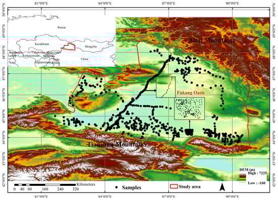
Figure 1.
Geographical location of the study area and distribution of sample sites (note: the red line is the boundary of the study area, not the national boundary).
2.2. Observation Data
In total, 709 surface soil samples (at 0–30 cm depth) were collected from the study area. The study adopted a different sampling strategy in the face of farmland and bare land. According to the measurement, the main land use type in the study area was bare land, which occupied 51.42% of the area, followed by grassland (33.85%) and farmland (11.73%). The samples of agricultural fields were mainly set up in the location of the field where the crop growth was uniform. The crop type of the plot was also representative of the surrounding vegetation. Three samples were collected from each plot and mixed to represent the characteristics of soil properties in that plot. In the grassland distribution area, the sample points were mainly considered for the sparseness of vegetation and the type of vegetation. The bare land in this study area is mainly semi-fixed desert, bare soil, bare rock, and salt soil (around lakes and in oases where the terrain is low). Since the feature cover characteristics are similar for several kilometers around the sampling locations, we collected only single samples in these areas.
In addition, with the help of the layout characteristics of the roads in this study area, we selected a southwest–northeast route. On this route, the study collected soil samples sequentially according to a 3 km step length. The samples collected under this route were able to cover most of the land cover types in this study area. At the same time, the study collected soils from different land use types and crop types in the area at the Fukang Oasis in the lower part of the Sankong River Basin. This site is also the location of the National Desert Field Observatory. With the above operations, the collected samples can capture the main features of geomorphological changes in the area.
Sampling was conducted in June 2019, July 2020, July 2021, and May 2022. The collected samples were scientifically processed and sent to the laboratory for measurement of soil organic carbon, soil salinity, and pH. Soil conductivity (μs/ms) and pH were identified at room temperature (25 °C) according to the prepared 1:5 hydric soil leachate using a digital multiparameter measurement device (Shanghai Leici DDS-11A/307A, Shanghai, China). SOC content (g/kg) was measured according to the modified Walkley–Black method [29]. Figure 2 shows the spatial distribution of soil properties (SOC, EC, and pH) at the sample sites in the northern part of Xinjiang.
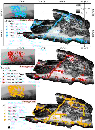
Figure 2.
Spatial distribution of soil properties (SOC, EC, and pH) at sample sites in the northern part of Xinjiang.
2.3. Satellite Data
The Sentinel-2 satellite, equipped with a multi-spectral imaging instrument covering 13 spectral bands, was selected for this study [30]. The satellite has a revisit period of 10 d for a single satellite and 5 d for the complementary revisit cycle of the A/B twin satellites. In terms of optical data, Sentinel-2 is the only satellite that has three bands in the red-edge range (visible, near-infrared, and shortwave infrared), making it ideal for land monitoring. Satellites can provide images of vegetation, soil, water cover, inland waterways, and coastal areas.
The MOD11A2 V6.1 product provides an average 8-d land surface temperature (LST) in a 1200 × 1200 km grid [31]. Each pixel value in MOD11A2 is an average of all corresponding MOD11A1 LST pixels collected within that 8-d period. The 8-d compositing period was selected because twice that period is the exact ground-track repeat period of the Terra and Aqua platforms. In this product, along with both the day- and nighttime surface temperature bands and their quality indicator layers, MODIS bands 31 and 32 and eight observation layers are also present. Specific information can be found at: https://doi.org/10.5067/MODIS/MOD11A2.061 (accessed on 1 September 2022).
The Sentinel-2 and MODIS data used in this study were acquired from 2019 to 2022.
2.4. Construction of a Water–Thermal–Spectral Dataset
This study aimed to develop a remote sensing dataset capable of capturing hydrothermal changes on the Earth’s surface. To achieve this, the study considered the hydrothermal characteristics and timing, which will be determined based on bioclimatic factors in the WorldClim dataset, and the local climate and observational data that can characterize the transition cycle between the dry and wet seasons. The bioclimatic factors used in the WorldClim dataset were BIO01-BIO10, which included the annual mean temperature (BIO01), mean diurnal range (BIO02), isothermality (BIO03), temperature seasonality (BIO04), maximum temperature of the warmest month (BIO05), minimum temperature of the cold month (BIO06), temperature annual range (BIO07), mean temperature of the wettest quarter (BIO08), mean temperature of the driest quarter (BIO09), and mean temperature of the warmest quarter (BIO10) (Table 1). These factors were selected to examine the potential impact of climate on hydrothermal changes and capture feedback information through remote sensing [18,19], which could be subsequently utilized for deducing land features. Furthermore, the study considered the dry–wet transition features of the local land surface. The dry–wet season transition cycle includes the transition cycles from the dry to wet season (February to May) and from the wet to dry season (July to October) [32,33,34]. To establish the dataset, we utilized various indicators, including Sentinel-2 bands (S2_b1 to S2_b12), as well as derived indices, such as normalized difference vegetation index (NDVI), enhanced vegetation index (EVI), and land surface water index(LSWI) [35]. Additionally, the study utilized daytime and nighttime temperatures from the MODIS 8-d composite dataset. Details of the methods employed are listed in Table 1.

Table 1.
WorldClim and local climate-inspired datasets of environmental variables for detecting hydrothermal variability based on Sentinel-2, MODIS, and bioclimatic variables. The varied colors are primarily for understanding.
Based on different time periods (different colors within a year span under Table 1), the study calculated the following indices that can reflect the hydrothermal changes of surface soil during the year. The meanings represented by the different acronyms are annotated under Table 1. Here, the study use MTWETQ_NDVI_MEDIAN/MAX (which follows the format: time period_index_calculation method) as an example to illustrate the meaning of the calculated variable. It means the median/max value of all available NDVIs for the three months of May, June, and July (refer to the time period covered by BIO08). The meanings represented by the other variables that follow in the manuscript can be understood in this way. In addition, DTW_326_416_LSWI means the study will count the median value of all available LSWIs for the 20 days from 26 March (3.26) to 16 April (4.16).
To compare the datasets established in this study, the study assembled the mean and maximum datasets, which are often used at large scales. The mean dataset was the mean value of the above participating variables from 2019 to 2022, whereas the maximum dataset was the maximum value of each parameter calculated from the available satellite data.
2.5. Background Data
Bioclimatic variables (19) were derived from the monthly temperature and rainfall data to generate biologically meaningful variables (WorldClim) [36,37]. These variables represented annual trends, seasonality, and extreme environmental factors. The average values of these variables were calculated for 1970–2000 and are commonly used in species distribution modeling and related ecological techniques [37]. Annual trends considered the mean annual temperature and annual precipitation, whereas seasonality included the annual range of temperature and precipitation. Extreme or limiting environmental factors included the temperature of the coldest and warmest months and precipitation of the wet and dry quarters, which are defined as a period of three months (1/4th of the year). These variables were downloaded from WorldClim.
In this study, climate data were obtained from the MODIS Terra Land Surface Temperature and Emissivity Daily Global Product reported by Hengl et al. [38]. Specifically, the study utilized daytime (temperature daytime monthly median), nighttime (temperature nighttime monthly median) land skin temperature data, day–night difference (temperature monthly day–night difference), as well as their standard deviations (temperature daytime monthly median) to gain a comprehensive understanding of the climatic conditions in the study area. The data were collected for 18 years, from 2000 to 2018, and presented in 12 bands representing 12 months of the year. A resolution of 1 km was selected, which allowed a comprehensive examination of the spatiotemporal patterns of the LST.
The change of the physical and chemical properties of the soil may have contributed to the changes in the land use and land cover (LULC), resulting in land degradation which, in turn, has led to a decline in soil productivity [39]. Land use data from 2017 were employed in our study. The land use types included in the data were agricultural land, forest land, grassland, shrubs, bare land, desert, water bodies, and wetlands [40].
Backscattering data were extracted from Advanced Land Observing Satellite-2/PALSAR-2 data with dual polarization (HH, HV) in the L-band and from Sentinel-1 mission data with single polarization (VV) in the C-band [41]. The synthetic aperture radar images underwent orthorectification and slope correction using the 90-m shuttle radar topography mission (SRTM) digital elevation model (DEM). To address intensity variations resulting from seasonal and daily changes in surface moisture conditions, a de-striping process based on Shimada et al. [42] was implemented. Previous studies have also demonstrated that the Sentinel-1 backscatter coefficient plays an important role in the inversion of information on soil moisture [43], crop type [44], soil salinity [45], flood [46], and above-ground biomass [47]. All these data are closely related to the soil properties of this study.
The SRTM-DEM was used as the terrain parameter. Furthermore, slope, multiresolution index of valley bottom flatness (MRVBF), topographic wetness index (TWI), and various topographic indices were derived from the DEM using the System for Automated Geoscientific Analyses (version 7.9) software [48]. The specific DEM-derived variables used are described in Wei et al. [49].
All of the aforementioned covariates (except land use) were procured from the Google Earth Engine (GEE) platform, which offers unparalleled planetary-scale geospatial analysis capabilities [50]. GEE also allows the resampling of environmental variables or remotely sensed-derived indices, enabling users to obtain the desired spatial resolution [21]. In our study, we set the resolution to 90 m, which appropriately balances the map details and computational time (Figure 3). All the data were downloaded and stacked as inputs to the model.
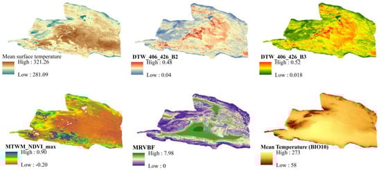
Figure 3.
Example maps of several environmental variables assessed in this study, including land use, climate, surface emissivity, and vegetation.
2.6. Machine Learning Algorithms
The Random Forest (RF) algorithm, introduced by Breiman [51], is a bagging-based ensemble learning approach that constructs multiple decision trees to model the relationships between independent and dependent variables for data classification and regression prediction. It integrates and selects important multiple feature values by building an extensive set of tree models, fully considering the significance of various feature values, selecting the optimal sample feature value to identify the best solution, and computing the average value of all predicted values as the final estimate. Compared with traditional regression prediction methods, RF can handle complex multi-dimensional feature values, thereby achieving higher accuracy in regression prediction. Consequently, RF have been broadly applied across various domains. The parameters and their values used in the RF modeling were as follows: the number of trees in the forest was 500, minimum sample split was 3, minimum sample leaf was 2, value of parameter “max_features” was 10, and the maximum depth was 40.
XGBoost is a machine learning algorithm based on gradient boosting trees that aims to iteratively optimize the loss function by gradually improving the model performance by adding new trees [52]. In each iteration, XGBoost calculates the contribution of each sample point to the current model, and then trains a new tree based on these contributions. Weighted least squares regression is an optimization strategy for regression problems that optimizes the model by minimizing the weighted average error, where the weights are the sample point weights. In addition to the optimization strategy, XGBoost employs several techniques to improve model performance and stability. One of the most important techniques is feature sampling, which randomly selects a subset of features to train each tree and reduces the risk of overfitting. Moreover, XGBoost uses techniques, such as sampling and cache optimization, to improve the algorithm efficiency. In summary, the core principle of the XGBoost algorithm is to optimize the model using gradient boosting trees while employing various techniques to improve the model performance and stability. The parameters in the model building process were set as follows: the maximum number of iterations was 1500, objective model was “squarederror”, booster was “gbtree”, random state was 1, and the maximum depth of a tree was 8.
LightGBM is an efficient and distributed gradient boosting tree-based machine learning algorithm developed by Microsoft [53]. It involves a gradient-based one-sided sampling (GOSS) and exclusive feature binding (EFB) process to aid training, and has shown good efficiency and scalability at high levels and large data volumes [54]. LightGBM uses a histogram-based algorithm that discretizes continuous feature values into s bins in floating-point format and uses these bins to construct histograms of width s. Since the histogram does not need to store pre-ordered results, it can find the best segmentation point during feature segmentation based on the cumulative statistics of each discrete value, thus effectively reducing memory consumption and computation time [55]. The core of LightGBM is an integrated learning algorithm that converts weak learners into strong learners, specifically by combining many low-accuracy tree models and employing gradient descent to reduce the loss function by moving to the negative gradient of the loss function at each iteration, ultimately producing a better tree as a prediction model [56]. Since the method searches a smaller portion of the sample rather than the entire data, it shows high efficiency and usually leads to comparable or better accuracy compared to other methods [57]. The parameters in the model construction process were as follows: the boosting type was “gbdt”, learning rate was 0.2, number of boosting iterations was 250, maximum depth was 30, maximum number of leaves in one tree was 500, and the minimum number of datapoints on a leaf was 1.
The RFE algorithm is widely used for selecting the most informative predictive variables for machine learning [58]. It operates based on the principle of backward selection, in which the least important variables are iteratively removed from the model until an optimal subset is obtained. Specifically, RFE involves the following steps: (1) A model is fitted using all pre-selected environmental variables, and its performance is evaluated using k-fold cross-validation to obtain variable importance measures. (2) The least important variable is removed based on its importance ranking, the model is re-fitted, and its performance is re-evaluated, and this process is repeated until the optimal subset is obtained. (3) The second step is repeated until only one variable remains, removing one variable at a time. (4) The optimal number of variables is determined based on the root mean square error (RMSE) criterion. The selected variables are subsequently fed into the XGBoost and LightGBM algorithms for further analysis. Notably, RFE was implemented using the RF model in the “caret” R package, which is a popular tool for machine learning and data mining.
The study also used structural equation modeling (SEM) to explore the complex causal relationships among the environmental factors, namely, SOC, pH, and electrical conductivity (EC). Based on previous research results, seven variables were considered for SEM analysis: rain, temperature, albedo (used to characterize soil-related properties, such assoil type), SOC, EC, NDVI, and pH. An SEM was constructed using the “lavaan” package in R software (3.5.3) [59].
2.7. Validation
To provide spatially robust predictions of surface soil properties and their associated uncertainties, the study utilized a bootstrap procedure [60] implemented within three machine learning algorithms, with 100 iterations performed for each algorithm, as described by van den Hoogen et al. [61]. Each bootstrap iteration randomly sampled 63% of the total soil observations for algorithm training [62], hyperparameter tuning, and spatial prediction, and the remaining 37% of the samples were used for validation. This occurs naturally through the “replacement sampling” mechanism of bootstrap samples. Each record has an equal chance of being drawn in as a bootstrap sample. Specifically, 100 covariate regressions were performed for all the soil properties [60]. In this way, less than 100 predictions were generated for each location and the mean value was calculated as the final prediction for that location. Then, the study compared the performance of the algorithms under different datasets based on the above process and selected the best algorithm for the final prediction of soil properties in the study area. According to Chen et al. [23], the study finally used all the samples to train the best model for the final mapping. The coefficient of variation (CV% = (standard deviation/mean prediction value) × 100) was used as a measure of the spatial uncertainty of our estimated mean-prediction accuracy or error [63]. Locations with larger CV values (greater variation around the mean predicted value) were deemed more uncertain, whereas smaller CV values were considered more accurate. The model performance was evaluated based on the coefficient of determination (R2) and RMSE.
3. Results
3.1. Statistical Summary of Key Soil Properties
The quantitative distribution of the soil samples was investigated based on land use categories (Figure 4). The statistical features of SOC revealed an upper limit of 68.76 g/kg, a lower limit of 0.49 g/kg, and an average of 8.30 g/kg. The median values illustrated that SOC was the highest in grasslands (11.84 g/kg), followed by agricultural lands (10.27 g/kg), shrublands (6.31 g/kg), and unused lands (4.56 g/kg). The maximum, minimum, and mean soil salinity values were 38,975, 37.40, and 1920 µs/cm, respectively. The median ranking of soil salinity indicated that shrublands (3294.74 µs/cm) had the highest soil salinity, followed by unused lands (2696.65 µs/cm), grasslands (2041.15 µs/cm), and agricultural lands (870.60 µs/cm). Further, the maximum, minimum, and mean pH values were 10.46, 6.58, and 8.46, respectively. The median statistical results demonstrated that the pH value of unused lands was the highest (8.66), followed by that of shrublands (8.59), grasslands (8.49), and agricultural lands (8.29).
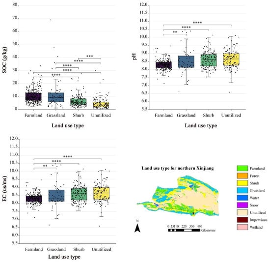
Figure 4.
Distribution characteristics of soil organic carbon (SOC), electrical conductivity (EC), and pH for various land use types. **: p < 0.05, ***: p < 0.01, ****: p < 0.0001.
Furthermore, the study recalculated the significance of land use effects on soil properties (Figure 4). For instance, with regards to SOC, there was no significant difference between farmland and grassland, but both exhibited significant differences when compared to shrub and unutilized land. The EC statistical characteristics indicated significant differences between farmland and other land types, but not between grassland, shrub, and unutilized land. This is because the northern Xinjiang region generally has low soil salinity, with highly salinized land types showing localized occurrences only, such as around Lake Ebey and Lake Manas, and in the lower terrain of the oasis. This similar mode of land use effects also occurred for pH. As a whole, the study area displayed an alkaline characteristic due to elevated calcium carbonate content in parent material [64]. Significant differences were found between agricultural areas and other land use types, which were attributed to the influence of human activities.
3.2. Performance Comparison of Three Datasets
Machine learning algorithms were employed in conjunction with median and mean datasets to evaluate the predictive accuracy of soil properties (Table 2). The findings indicated that the optimal predictive accuracy for the three key soil properties, namely SOC, EC, and pH, was achieved with R2 values of 0.40, 0.41, and 0.40, respectively, and RMSEs of 4.71 g/kg, 2842.28 µs/cm, and 0.37, respectively. Notably, the prediction accuracies of SOC and EC with the support of the median datasets were significantly higher than those of the maximum value datasets. Conversely, the pH prediction accuracy under the support of the maximum value datasets was superior to that of the median datasets.
Table 2.
Performance of the three distinct datasets of soil organic carbon (SOC), electrical conductivity (EC), and pH, when combined with machine learning algorithms.
This study revealed that the overall predictive accuracy of the newly established dataset was higher than that of the median and mean datasets (Figure 5). Among all predictive results, EC exhibited the highest explanatory accuracy (R2 = 0.54 (LightGBM)), followed by SOC (R2 = 0.48 (LightGBM)). The pH modeling results under RF support explained 44% of the data variability. However, all verification results of the key soil properties confirmed a significant correlation between the predicted and observed values (p < 0.0001). Moreover, residuals exhibited a random distribution.
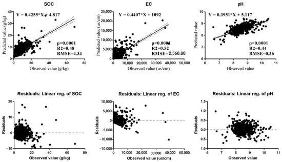
Figure 5.
Scatterplots depicting the relationship between predicted and observed values, as generated by the optimal model.
The study utilized all available samples and extracted digital soil maps prepared by previous researchers, which were then used to validate their respective models within the study area (Figure 6). Unfortunately, none of the results could explain the spatial variability in the key soil properties observed across our study area. The scatterplots of the predicted and observed values also did not provide any discernible patterns. For example, the R2 value for SoilGrid250_SOC was only 0.03, whereas its corresponding scatterplot manifested observed values predominantly clustered within the range of 0–20, even though SoilGrid250_SOC exhibited a value range distributed much more widely, from 0 to 50. The HWSD_EC and Ivushkin et al. [22] soil salinity maps were available for public download; however, their respective R2 values remained low (0.00 and 0.02, respectively). When comparing our pH model with three other products, HWSD_T_pH, SoilGrid_pH, and Chen et al._pH [23], none of the resulting digital soil maps could explain the spatial variability of pH within our study area, with the R2 values being almost zero.
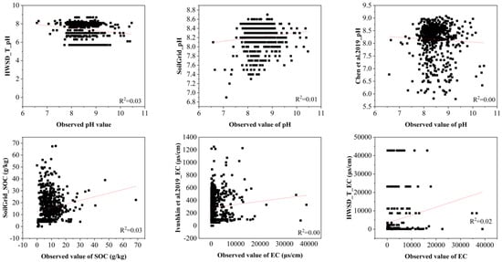
Figure 6.
Validation of the precision of datasets, including SoilGrid250 and HWSD products, as well as findings of other studies, which are available for public download in Northern Xinjiang, using the collected samples collected for SOC, EC, and pH.
3.3. Important Variables
Figure 7 shows the variables selected to predict the target soil properties. Through RF iterative computation, the study also determined an importance ranking of key soil properties that affected SOC prediction, thus allowing us to identify the optimal dataset for predicting SOC based on RMSE and R2 metrics. Our findings revealed that a dataset consisting of 20 variables was the optimal combination for predicting SOC, with variable selection achieved by balancing model uncertainty and reducing the number of variables. The five most important variables were BIO10, Longterm_Mean_D_FEB, BIO08, BIO01, and MTWETQ_NDVI_MEDIAN. Notably, when 13 variables were predicted, the accuracy of soil salinity modeling reached a maximum R2 value while the RMSE was minimum. Further analysis indicated that DTW2021_406-426_B3, DTW2021_826-916_B12, Temperature Daytime Monthly_Median_NOV, Temperature Monthly Day-nights Difference_OCT, and Temperature Daytime Monthly_Median_JUN were the top five most important variables for predicting soil salinity. For pH, the minimum RMSE and R2 values were obtained with a variable count of 15. By ranking the variables, the study found that land use type was the most pertinent variable, followed by WTD2021_906_926_NDVI, WTD2021_816_906_B2, Temperature Daytime Monthly Median_JAN, and TAR_NDVI_MAX.
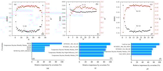
Figure 7.
Selected variables for predicting SOC, EC, and pH within the study area, which were obtained through iteration of the RFE algorithm. The upper three figures (a–c) show the criteria used to determine the number of variables for SOC, EC and pH, whereas the lower three figures (d–f) show the selected top five variables for SOC, EC and pH. Please read Section 3.3 and Section 3.4 for the meanings of the variables.
Figure 8 shows the correlations between the preferred and key attributes. BIO10 and ISO_B8 showed the strongest correlations with SOC (correlation coefficient, r = 0.36 and −0.36, respectively). For EC, the top three correlations were associated with the red, green, and blue bands acquired in spring (426_426) with corresponding r values of 0.45, 0.44, and 0.41, respectively. Lastly, NDVI obtained in autumn (906_926) showed the highest correlation with pH (r = −0.41), followed closely by TAR_NDVI_MAX (r = −0.39) and the red band (B4) obtained in autumn (821_911).

Figure 8.
Correlations between SOC, EC, and pH and the preferred environmental variables.
SEM assumed a causal relationship between the environmental variables considered in the analysis and simultaneously assessed the direct and indirect effects among the variables (Figure 9). Regarding the absolute values of the path coefficients, MAT and surface reflectance emerged as the primary factors influencing EC, with the latter exerting a greater impact. pH had the most substantial negative effect on SOC, followed by MAT, whereas an increase in rainfall was positively associated with SOC. Furthermore, NDVI might have augmented SOC levels by reducing EC. Notably, an increase in NDVI reduced the pH, whereas surface reflectance increased the pH.
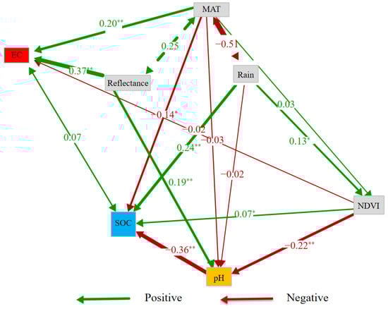
Figure 9.
SEM-based quantification of the relationships between the environmental variables (SOC, EC, and pH) within the study area. *: p < 0.05, ** p < 0.01. Green arrows represent negative relationships and red arrows represent positive relationships.
3.4. Spatial Distribution of SOC, EC, and pH
Figure 10 displays the spatial distribution maps of the predicted values for the three critical parameters, indicating that regions with high uncertainty were relatively limited in extent, and the CV values were within a range of moderate variability. Interestingly, high uncertainty values for the SOC and EC prediction maps occurred primarily in the vicinity of the oases located near the Tianshan Mountains. The CV value map for pH exhibited no distinct areas with high uncertainty, indicating relatively stable predictions. Collectively, these findings underscored the robustness of the prediction models for the parameters studied. Nevertheless, future studies should consider incorporating more variables or refining the model accuracy to further minimize prediction uncertainties.
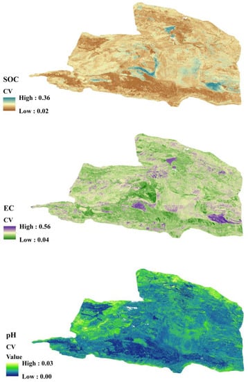
Figure 10.
Spatial uncertainty (CV) of the predicted soil attributes (SOC, EC, and pH).
Figure 11 shows the spatial distribution of the predicted key properties after 100 iterations. The visualization revealed that regions with high SOC content were predominantly located in hilly and mountainous regions, including the grasslands of the Altai and Tianshan Mountains. Contrastingly, the central region of the Junggar Basin exhibited low SOC content. Soil salinization was identified as a primary factor impacting ecological security in the study area and has also been prevalent in wetlands around Lake Ebi [65], dried-up tail lakes in the Manas River Basin [66], and swamps and wetlands near Lake Fuhai in the north of the study area [67]. The eastern region of the Junggar Basin is characterized by relatively higher alkalinity, whereas the hilly and mountainous areas exhibit lower pH values. The geochemical composition of the produced water in the Junggar Basin was assessed [68], and Cl−, Na+, and HCO3− were found to be the principal controllers of the total dissolved solid (TDS) content within the produced water. Furthermore, their concentrations increased with the depth of water. Moreover, a correlation existed between the increased pH and TDS levels. Further, we compared the results of the mean values of the three soil attributes calculated in this study with those of other research teams (Figure 12). The results showed that although the spatial distributions of SOC and EC were similar, the data ranges were more variable. pH had a similar range of value domains, but there was some variability in the spatial ranges.
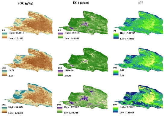
Figure 11.
Predicted P5 (upper), P50 (median), and P95 (lower) values of SOC, EC, and pH at 90-m resolution.
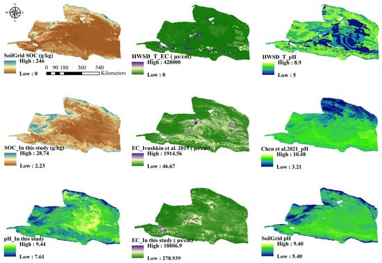
Figure 12.
Spatial distribution maps of SOC, EC, and pH produced by various research groups within our study area [22,23].
4. Discussion
4.1. Characteristics of Soil Properties under Different Land Uses
Our findings showed that the highest SOC content was in the grasslands, followed by farmlands, whereas bare land, such as deserts and exposed rocks, displayed the lowest SOC content (Figure 4). Plant residues were the primary sources of SOC in grasslands. Moreover, grasslands with high vegetation cover were influenced by location-specific climatic conditions, good soil quality, and slow organic matter decomposition. Additionally, the rich diversity of surface vegetation combined with high coverage facilitated the importance of significant quantities of vegetation residue and organic matter into the soil, thereby increasing organic carbon levels. Multiple studies have confirmed that soils under natural vegetation cover exhibit decreasing levels of soil organic matter after cultivation [69]. Carbon loss from such soils has been estimated to range between 30% and 50% after converting grasslands into agricultural lands [70,71]. Wastelands and bare lands, which remain in their natural state for extended periods, lack surface vegetation and possess inadequate water and nutrient retention abilities. Consequently, the soil surfaces of such lands characteristically receive much less organic matter, leading to low organic carbon contents.
Soil salinity and alkalinity are crucial properties influenced by biological, climatic, geological, and hydrological factors during formation. Overall, our study area was characterized as alkaline. However, extremely hypersaline zones were present in certain regions, such as Lakes Manas and Ebi (Figure 11) This was predominantly determined by the parent rock properties in the study area; moreover, high evaporation rates have also been confirmed as influencing factors [10].
4.2. Impact of Three Datasets on Soil Property Modeling
Environmental variables derived from the mean or maximum values of remote sensing data over a year may not fully capture the surface reflectance fluctuations that occur throughout the year. Compared with the two datasets mentioned above (Table 2), the optimal model established based on our newly created dataset demonstrated a 25%, 31.79%, and 5% improvement in the R2 value for SOC, EC, and pH predictions, respectively; additionally, the RMSE decreased by 7.86%, 11.67%, and 5.26%, respectively. These results demonstrated the superiority of our dataset in predicting soil properties and highlighted the importance of capturing comprehensive temporal changes in surface reflectance for accurate predictions. Digital mapping of SOC has garnered significant attention from the scientific community. Therefore, the present study compared our findings with the results of previous studies in the same research domain. For instance, the validation outcomes reported by Simbahan et al. [72] revealed that the RMSE of SOC was 9.6, while the mean absolute error was 7.1. Similarly, Kumar et al. [73] yielded an R2 value of 0.36 and a mean error of 0.23. Additionally, the RMSE and R2 complied from other pertinent studies were RMSE = 68.7 and R2 = 0.27 [74], R2 = 0.28 and RMSE = 6.74 [75], RMSE = 5.63 [76], and R2 = 0.44 and RMSE = 9.16 [77].
4.3. Temporal Characteristics of Surface Hydrological and Climatic Features
The model comparison results confirmed our initial hypothesis that seasonal fluctuations in hydrothermal parameters and their feedback at the surface are potential drivers; additionally, the study found hydrothermal variability patterns in the arid zone by reviewing the literature. Several studies conducted in the inland arid regions of China, when the wet (April–November) and dry (November–April) seasons alternate in the dry zone, have highlighted the impact of seasonal variations on various parameters, including temperature, precipitation, soil temperature, and soil moisture [32,33,34]. For instance, observations from the Heihe River Basin meteorological station in an inland arid region showed a steady increase in evapotranspiration values from the beginning of the year, which accelerated in late February, peaked in May, oscillated at a high level from June to August, and rapidly declined from August to September, before slowing from September to October [78]. Groundwater monitoring data have also declined continuously in the groundwater table from March to early June as a result of irrigation practices [79]. Gao et al. [33] found that monthly precipitation in northern Xinjiang exhibited a significant increasing trend from March to May and a continuous decreasing trend from August to October. Similarly, Li et al. [80] discovered that soil moisture in the cotton planting area of southern Xinjiang decreased from March to May at a depth of 0–20 cm and fluctuated within a range from June to August before continuously declining from August to October. Su et al. [81] and Tian et al. [82] also reported that soil moisture gradually decreased from February to May and increased from August to November, based on in situ soil moisture monthly records from the Shache station in the Tarim River basin and soil moisture data from meteorological stations across Xinjiang. Further, June and July exhibited the lowest soil moisture levels throughout the year. Tian et al. [82] analyzed the soil moisture and temperature characteristics of Haloxylon ammodendron forests of different ages in the Hexi Corridor of Northwest China and found that during February–May, the soil temperature increased from 2.52 °C to 22.80 °C, while the soil moisture increased from 2.1% to 8.37%. Tian et al. [82] demonstrated multi-spectral temporal changes in typical land cover types in the Sangong River Basin in northern Xinjiang and reported a rapid increase in spectral reflectance from March to May, whereas grasslands and bare soil exhibited a slow decline from August to October. The reflectance of corn and rice increased gradually, whereas those of grapes and cotton decreased slowly at a low level; moreover, wheat and oil sunflowers exhibited relatively rapid declines. To incorporate these seasonal variations in hydrothermal parameters and land cover changes into the models, variables, such as climate, remote sensing, and vegetation, were calibrated over time.
4.4. Comparing the Prediction Results of This Study with the Products of Other Research Groups
The discrepancy between the validation accuracy of the reference products and the modeling accuracy in our study may stem from the type of variables selected and the temporal effects of the samples. Given the global scale of this investigation, the study scrutinized the variables utilized in the generation models of SoilGrid250_SOC and SoilGrid250_pH, which predominantly originated from long-term MODIS products (1000 m, 2000–2017). This issue was also apparent in the pH products developed by Chen et al. (2019) [23] and EC products formulated by Ivushkin et al. (2019) [22]. Furthermore, sample data employed in these studies were relatively sparse in our study area, as the models for their corresponding products were established based on samples from other regions of China or the world. In addition, the sampling time (the 1980s) and satellite imaging time (since 2000) were not synchronous, which inevitably impaired the transferability of the models. However, these limitations can be attributed to objective factors that were beyond our control. Nevertheless, these products provide indispensable contributions to global land models and the evolution of environmental ecology.
In this study, the study extracted products from different research teams based on the boundaries of the study area and used them for comparison with the key attribute maps produced in our research (Figure 12). Notably, the SoilGrid SOC product exhibited a clear difference from the SOC map generated in our study in terms of numerical range, with the former having a significantly higher maximum value. However, the spatial distribution characteristics of both the products shared some similarities. A comparison of the EC products showed significant differences in both numerical range and spatial distribution, with HWSD_T_EC having a similar spatial distribution range as our study but with larger maximum and high-value ranges. Notably, highly saline areas were not restricted to the wetlands around Ebi Lake, but also included the transitional zone between the oasis and desert in the southern part of the study area where salt was discharged. In terms of the EC_ivuskin et al. (2019) prediction map [22], the maximum pH value was significantly lower than that predicted in our study, although the region with the maximum value was similar to our results. To compare the results of our study with those of other pH products, the study utilized three pH products: soilGrid_pH, an upgraded product of HWSD_T_pH. The latter was significantly different from our study in terms of the maximum value, which was observed in mountainous areas, and the minimum value, which was observed in deserts, thus, deviating significantly from the actual conditions. Contrastingly, the low-value areas reported by [23] were consistent with the values of our study, whereas the high-value areas demonstrated no clear features. Despite sharing a spatial pattern similar to that found in our study, soilGrid_pH exhibited a smaller minimum value than the predicted minimum value. However, the difference in pH between the desert and oases was smaller in soilGrid_pH than that in our study.
4.5. Environmental Influences on Soil Properties and Insights
The contribution of climate-related variables to the variations in SOC was paramount, followed closely by the vegetation index and surface reflectance. Among the variables in the SOC modeling dataset, approximately 55% were associated with climate, and climate-related variables accounted for 63% and 40% of the variations in EC and pH, respectively. The significance of climate originates from its role in shaping plant types and soil conditions as it affects carbon input and waste decomposition [83]. Furthermore, SOC accumulation is promoted in regions with high rainfall and low temperatures, enabling carbon and nitrogen storage in soils [84]. The high SOC concentrations observed in the mountainous or high-altitude hilly areas in our study can be explained by these conditions. Microbial decomposition of organic matter is inhibited by low temperatures, which affects SOC content [85]. The annual average temperature is a robust predictor of SOC content in several regions [86], including Europe [87], the black soil region of Northeast China [88], and the Brazilian tropical region [89]. Additional climate parameters, such as maximum and minimum temperatures, maximum and minimum precipitation, and remote sensing indices related to water, have also been used to explain SOC variability [90]. However, our study underscored the critical role of average temperature in the hottest quarter (June–August) and surface temperature in February, which represented two extreme thermal conditions influencing the SOC content. High temperatures can decline or stop photosynthesis in plants, and increase respiration [91], with respiration rates exceeding the decrease in vegetation productivity, thereby exacerbating the decline in ecosystem carbon sink functions. Further, low temperatures can impede plant growth [92], and freezing can cause cell dehydration, resulting in plant tissue damage or mortality [93].
The findings of this study indicated a negative correlation between soil pH and SOC content. Soil pH affects microbial activity and plays a crucial role in shaping the decomposition and mineralization processes of organic carbon [94]. The suppressed level of microbial activity in acidic soils causes sluggish decomposition of organic carbon [95]. However, as the soil pH increases, the decomposition rate accelerates, resulting in less organic matter accumulation [96]. Research has demonstrated that precipitation positively influences SOC content in other geographical regions as well [97], thereby enhancing plant productivity. Consequently, increasing the input rates of organic matter and nitrogen contributes to SOC storage.
Based on our SEM analysis and identification of important variables, the study determined that land surface reflectance and temperature played key roles in spatially characterizing the EC in our study area. Interestingly, both spring and autumn were critical periods for EC inversion in this region, which may be closely associated with local hydrological changes. Specifically, in April, the groundwater level reaches its highest point, leading to salinization of the surface soil due to evaporation during the subsequent spring warming [98,99]. In autumn, after irrigation and evaporation occur throughout the growing season, the salt content (0–30 cm) returns to the surface with initial seepage [100,101]. Thus, in agricultural lands within this region, desalination treatment is typically conducted after harvest [102]. Thus, the study can conclude that the spatial distribution of salinization in the study area was relatively stable. Therefore, the salinity inversion results acquired when there was no vegetation cover in spring can provide a reliable reference for salt distribution during the crop growth season, which is important for irrigation and salt management decision-making.
The use of an NDVI and land use data acquired in autumn is a valuable resource for predicting the spatial distribution of soil pH in the study area, thus, highlighting the significant influence of vegetation on pH levels. Müller et al. [103] demonstrated that land utilization and management practices have a profound impact on soil pH values, indicating that grassland soils exhibit stronger acidity than agricultural fields because of the addition of industrial lime and fertilizer, which promote the formation of carbonates, leading to low pH levels. Conversely, organic matter returns to the soil via litter layers in forested areas, subsequently decreasing soil pH through nitrogen mineralization and nitrification [104,105]. Additionally, root-associated fungi and mycorrhizae in forests affect soil pH levels and accelerate the weathering of carbonate rocks [106]. The variance in the organic matter content and root exudate input of different soil types underscores the uniqueness of forest soils compared to other soil types [107]. Furthermore, by extracting vegetation information from variable importance analyses, such as NDVI data obtained from autumn imagery, researchers have gained insights into leveraging remote sensing technology to differentiate spectral variations among various plant species. These findings provide a critical understanding of the effects of vegetation on soil chemistry, sustainable land management practices, and ecosystem conservation strategies.
4.6. More Corroboration and Research Are Needed for the Changes in Soil Properties in Northern Xinjiang
After comparing the historical data, the study found that climate warming significantly influenced soil properties. The products cited in our study represented the spatial variability of soil properties in the 1980s owing to the sampling time. To evaluate the potential impacts of climate change, the study calculated the mean values of the products that were spatially similar to those used in our study. The mean SOC value of SoilGrid250 (15.70) was higher than that reported in our study (8.29), while the mean EC value of HWSD_T_EC and that found in our study were 4051.96 and 1920, respectively. The mean pH values of SoilGrid_pH, Chen et al. 2019_pH, and the present study were 8.23, 8.19, and 8.46, respectively. This indicated that, compared to the 1980s, the mean SOC and EC values significantly decreased. The decrease in pH was less significant than that in SOC and EC but was still noticeable. According to the variable importance, temperature is the key factor controlling the properties of the study area. When the study examined the climate history, the study found that the warming rate of the mean temperature of 89 stations in Xinjiang during 1961–2018 was 0.30 (p < 0.01). The contribution of winter warming is the largest [108]. The average minimum temperature (Tmin) and maximum temperature (Tmax) are both significantly increasing at rates of 0.44 and 0.22 °C/decade, respectively [108]. Climate warming has increased extreme warm events and decreased extreme cold events. Furthermore, the warming rate has decreased from north to south, and the largest warming amplitude has been reported in the northern part of Xinjiang (the study area) and mountainous areas [109]. Hobley et al. [110] reported a negative correlation between temperature and SOC. The decrease in EC may be related to oasis expansion and excessive extraction of groundwater [111,112,113].
Here, this study only examined the changes in soil properties by product comparison. The results generated by this are just our speculation. However, more historical data are needed to verify whether the changes actually occurred.
5. Conclusions
To advance our understanding of the spatial distribution of the key soil properties in northern Xinjiang, this study developed a prediction model based on a novel dataset that captured the temporal dynamics of a water–heat–spectral reflectance database under extreme climates and dry–wet conversion processes. This dataset allowed us to indirectly infer the soil variability and its association with key properties. The validation of the prediction results of our model provided valuable insights. The results of this study revealed that the relatively optimal modeling algorithms for SOC, EC, and pH are LightGBM, RF, and LightGBM, respectively, under the support of the median dataset. Secondly, the relatively optimal modeling algorithms corresponding to the three soil attributes with the support of the maximum value dataset are RF, LightGBM, and LightGBM, respectively. With the support of the newly created dataset in this study, LightGBM performed the best, followed by RF. It can be seen that different algorithms need to be tried continuously to obtain the optimal model under different environmental qualities. No algorithm performed well under all conditions. This study also found that the predictive performance of our newly established model surpassed that of commonly used mean or maximum value datasets. This underscored the importance of incorporating temporal dynamics into soil prediction models. Furthermore, our prediction results showed a significant decrease in the mean SOC and EC values compared to soil properties that were more representative of the history, whereas the change in pH value was not significant.
Author Contributions
Conceptualization, F.W., Y.W. and S.Y.; methodology, F.W. and Y.W.; validation, F.W.; data curation, Y.W.; visualization, F.W. and S.Y.; writing—original draft; F.W. and Y.W.; writing—review and editing, Y.W. and S.Y.; funding acquisition, F.W. and S.Y. All authors have read and agreed to the published version of the manuscript.
Funding
This study was supported by the National Natural Science Foundation of China (Grant Numbers: 42101363 and U1603241). We also thank the graduate students who worked hard in soil sampling and sample processing.
Data Availability Statement
The data in this study are available from the corresponding authors upon request.
Conflicts of Interest
The authors declare no conflict of interest.
References
- Ma, Y.; Minasny, B.; Malone, B.P.; Mcbratney, A.B. Pedology and digital soil mapping (DSM). Eur. J. Soil. Sci. 2019, 70, 216–235. [Google Scholar] [CrossRef]
- Chen, S.; Arrouays, D.; Leatitia Mulder, V.; Poggio, L.; Minasny, B.; Roudier, P.; Libohova, Z.; Lagacherie, P.; Shi, Z.; Hannam, J.; et al. Digital mapping of GlobalSoilMap soil properties at a broad scale: A review. Geoderma 2022, 409, 115567. [Google Scholar] [CrossRef]
- Mathieu, R.; Pouget, M.; Cervelle, B.; Escadafal, R. Relationships between satellite-based radiometric indices simulated using laboratory reflectance data and typic soil color of an arid environment. Remote Sens. Environ. 1998, 66, 17–28. [Google Scholar] [CrossRef]
- Palacios-Orueta, A.; Ustin, S.L. Remote sensing of soil properties in the Santa Monica Mountains I. Spectral analysis. Remote Sens. Environ. 1998, 65, 170–183. [Google Scholar] [CrossRef]
- Grimm, R.; Behrens, T.; Märker, M.; Elsenbeer, H. Soil organic carbon concentrations and stocks on Barro Colorado Island—Digital soil mapping using Random Forests analysis. Geoderma 2008, 146, 102–113. [Google Scholar] [CrossRef]
- McBratney, A.B.; Santos, M.M.; Minasny, B. On digital soil mapping. Geoderma 2003, 117, 3–52. [Google Scholar] [CrossRef]
- Taghizadeh-Mehrjardi, R.; Hamzehpour, N.; Hassanzadeh, M.; Heung, B.; Goydaragh, M.G.; Schmidt, K.; Scholten, T. Enhancing the accuracy of machine learning models using the super learner technique in digital soil mapping. Geoderma 2021, 399, 115108. [Google Scholar] [CrossRef]
- Taghizadeh-Mehrjardi, R.; Sheikhpour, R.; Zeraatpisheh, M.; Amirian-Chakan, A.; Toomanian, N.; Kerry, R.; Scholten, T. Semi-supervised learning for the spatial extrapolation of soil information. Geoderma 2022, 426, 116094. [Google Scholar] [CrossRef]
- Scudiero, E.; Skaggs, T.H.; Corwin, D.L. Regional-scale soil salinity assessment using Landsat ETM + canopy reflectance. Remote Sens. Environ. 2015, 169, 335–343. [Google Scholar] [CrossRef]
- Wang, F.; Yang, S.; Wei, Y.; Shi, Q.; Ding, J. Characterizing soil salinity at multiple depth using electromagnetic induction and remote sensing data with random forests: A case study in Tarim River Basin of southern Xinjiang, China. Sci. Total Environ. 2021, 754, 142030. [Google Scholar] [CrossRef]
- Wang, N.; Peng, J.; Xue, J.; Zhang, X.; Huang, J.; Biswas, A.; He, Y.; Shi, Z. A framework for determining the total salt content of soil profiles using time-series Sentinel-2 images and a random forest-temporal convolution network. Geoderma 2022, 409, 115656. [Google Scholar] [CrossRef]
- Fathololoumi, S.; Vaezi, A.R.; Alavipanah, S.K.; Ghorbani, A.; Saurette, D.; Biswas, A. Improved digital soil mapping with multitemporal remotely sensed satellite data fusion: A case study in Iran. Sci. Total Environ. 2020, 721, 137703. [Google Scholar] [CrossRef] [PubMed]
- Lobell, D.B.; Lesch, S.M.; Corwin, D.L.; Ulmer, M.G.; Anderson, K.A.; Potts, D.J.; Doolittle, J.A.; Matos, M.R.; Baltes, M.J. Regional-scale Assessment of Soil Salinity in the Red River Valley Using Multi-Year MODIS EVI and NDVI. J. Environ. Qual. 2010, 39, 35–41. [Google Scholar] [CrossRef] [PubMed]
- Wu, W.; Mhaimeed, A.S.; Al-Shafie, W.M.; Ziadat, F.; Dhehibi, B.; Nangia, V.; De Pauw, E. Mapping soil salinity changes using remote sensing in Central Iraq. Geoderma Reg. 2014, 2–3, 21–31. [Google Scholar] [CrossRef]
- Yang, L.; Cai, Y.; Zhang, L.; Guo, M.; Li, A.; Zhou, C. A deep learning method to predict soil organic carbon content at a regional scale using satellite-based phenology variables. Int. J. Appl. Earth. Obs. 2021, 102, 102428. [Google Scholar] [CrossRef]
- Zhang, T.-T.; Qi, J.-G.; Gao, Y.; Ouyang, Z.-T.; Zeng, S.-L.; Zhao, B. Detecting soil salinity with MODIS time series VI data. Ecol. Indic. 2015, 52, 480–489. [Google Scholar] [CrossRef]
- Liu, F.; Geng, X.; Zhu, A.X.; Fraser, W.; Waddell, A. Soil texture mapping over low relief areas using land surface feedback dynamic patterns extracted from MODIS. Geoderma 2012, 171–172, 44–52. [Google Scholar] [CrossRef]
- Liu, F.; Rossiter, D.; Song, X.-D.; Zhang, G.L.; Wu, H.; Zhao, Y. An approach for broad-scale predictive soil properties mapping in low-relief areas based on responses to solar radiation. Soil. Sci. Soc. Am. J. 2020, 84, 144–162. [Google Scholar] [CrossRef]
- Zeng, C.; Qi, F.; Zhu, A.X.; Liu, F. Construction of land surface dynamic feedback for digital soil mapping considering the spatial heterogeneity of rainfall magnitude. Catena 2020, 191, 104576. [Google Scholar] [CrossRef]
- Hengl, T.; Jesus, J.M.D.; Macmillan, R.A.; Batjes, N.H.; Heuvelink, G.B.M.; Ribeiro, E.; Samuelrosa, A.; Kempen, B.; Leenaars, J.G.B.; Walsh, M.G. SoilGrids1km Global Soil Information Based on Automated Mapping. PLoS ONE 2014, 9, e105992. [Google Scholar] [CrossRef]
- Hengl, T.; Mendes, d.J.J.; Heuvelink, G.B.; Ruiperez, G.M.; Kilibarda, M.; Blagotić, A.; Shangguan, W.; Wright, M.N.; Geng, X.; Bauermarschallinger, B. SoilGrids250m: Global gridded soil information based on machine learning. PLoS ONE 2017, 12, e0169748. [Google Scholar] [CrossRef] [PubMed]
- Ivushkin, K.; Bartholomeus, H.; Bregt, A.K.; Pulatov, A.; Kempen, B.; de Sousa, L. Global mapping of soil salinity change. Remote Sens. Environ. 2019, 231, 111260. [Google Scholar] [CrossRef]
- Chen, S.; Liang, Z.; Webster, R.; Zhang, G.; Zhou, Y.; Teng, H.; Hu, B.; Arrouays, D.; Shi, Z. A high-resolution map of soil pH in China made by hybrid modelling of sparse soil data and environmental covariates and its implications for pollution. Sci. Total Environ. 2019, 655, 273–283. [Google Scholar] [CrossRef] [PubMed]
- Wei, W.; Guo, Z.; Shi, P.; Zhou, L.; Wang, X.; Li, Z.; Pang, S.; Xie, B. Spatiotemporal changes of land desertification sensitivity in northwest China from 2000 to 2017. J. Geogr. Sci. 2021, 31, 46–68. [Google Scholar] [CrossRef]
- Pi, H.; Sharratt, B.; Lei, J. Atmospheric dust events in central Asia: Relationship to wind, soil type, and land use. J. Geophys. Res-Atmos. 2017, 122, 6652–6671. [Google Scholar] [CrossRef]
- Chai, H.; Zhou, C.; Chen, X.; Cheng, W. Digital regionalization of geomorphology in Xinjiang. J. Geogr. Sci. 2009, 19, 600. [Google Scholar] [CrossRef]
- Hu, T.; Hu, Y.; Dong, J.; Qiu, S.; Peng, J. Integrating Sentinel-1/2 Data and Machine Learning to Map Cotton Fields in Northern Xinjiang, China. Remote Sens. 2021, 13, 4819. [Google Scholar] [CrossRef]
- O’Brien, D.; Primiano, C.B. Opportunities and risks along the New Silk Road: Perspectives and perceptions on the Belt and Road Initiative (BRI) from the Xinjiang Uyghur Autonomous Region. In International Flows in the Belt and Road Initiative Context: Business, People, History and Geography; 2020; pp. 127–145. Available online: https://link.springer.com/chapter/10.1007/978-981-15-3133-0_6 (accessed on 4 July 2023).
- Nelson, D.A.; Sommers, L.E. Total carbon, organic carbon, and organic matter. In Methods of Soil Analysis: Part 2 Chemical and Microbiological Properties; 1983; Volume 9, pp. 539–579. Available online: https://acsess.onlinelibrary.wiley.com/doi/abs/10.2134/agronmonogr9.2.2ed.c29 (accessed on 4 July 2023).
- Drusch, M.; Del Bello, U.; Carlier, S.; Colin, O.; Fernandez, V.; Gascon, F.; Hoersch, B.; Isola, C.; Laberinti, P.; Martimort, P. Sentinel-2: ESA’s optical high-resolution mission for GMES operational services. Remote Sens. Environ. 2012, 120, 25–36. [Google Scholar] [CrossRef]
- Wan, Z.; Dozier, J. A generalized split-window algorithm for retrieving land-surface temperature from space. IEE T Geosci. Remote 1996, 34, 892–905. [Google Scholar]
- Huang, X.; Bao, A.; Guo, H.; Meng, F.; Zhang, P.; Zheng, G.; Yu, T.; Qi, P.; Nzabarinda, V.; Du, W. Spatiotemporal changes of typical glaciers and their responses to climate change in Xinjiang, Northwest China. J. Arid. Land. 2022, 14, 502–520. [Google Scholar] [CrossRef]
- Gao, F.; Zhang, Y.; Chen, Q.; Wang, P.; Yang, H.; Yao, Y.; Cai, W. Comparison of two long-term and high-resolution satellite precipitation datasets in Xinjiang, China. Atmos. Res. 2018, 212, 150–157. [Google Scholar] [CrossRef]
- Yao, S.; Jiang, D.; Zhang, Z. Moisture sources of heavy precipitation in Xinjiang characterized by meteorological patterns. J. Hydrometeorol. 2021, 22, 2213–2225. [Google Scholar] [CrossRef]
- Xiao, X.; Boles, S.; Frolking, S.; Salas, W.; Moore Iii, B.; Li, C.; He, L.; Zhao, R. Observation of flooding and rice transplanting of paddy rice fields at the site to landscape scales in China using VEGETATION sensor data. Int. J. Remote Sens. 2002, 23, 3009–3022. [Google Scholar] [CrossRef]
- Fick, S.E.; Hijmans, R.J. WorldClim 2: New 1-km spatial resolution climate surfaces for global land areas. Int. J. Climatol. 2017, 37, 4302–4315. [Google Scholar] [CrossRef]
- Hijmans, R.J.; Cameron, S.E.; Parra, J.L.; Jones, P.G.; Jarvis, A. Very high resolution interpolated climate surfaces for global land areas. Int. J. Climatol. 2005, 25, 1965–1978. [Google Scholar] [CrossRef]
- Hengl, H.; Kluger-Eigl, W.; Blab, R.; Füssl, J. The performance of paving block structures with mortar filled joints under temperature loading, accessed by means of numerical simulations. Road. Mater. Pavement 2018, 19, 1575–1594. [Google Scholar] [CrossRef]
- Biro, K.; Pradhan, B.; Buchroithner, M.; Makeschin, F. Land use/land cover change analysis and its impact on soil properties in the northern part of Gadarif region, Sudan. Land. Degrad. Dev. 2013, 24, 90–102. [Google Scholar] [CrossRef]
- Gong, P.; Liu, H.; Zhang, M.; Li, C.; Wang, J.; Huang, H.; Clinton, N.; Ji, L.; Li, W.; Bai, Y.; et al. Stable classification with limited sample: Transferring a 30-m resolution sample set collected in 2015 to mapping 10-m resolution global land cover in 2017. Sci. Bull. 2019, 64, 370–373. [Google Scholar] [CrossRef]
- Guan, K.; Li, Z.; Rao, L.N.; Gao, F.; Xie, D.; Hien, N.T.; Zeng, Z. Mapping paddy rice area and yields over Thai Binh Province in Viet Nam from MODIS, Landsat, and ALOS-2/PALSAR-2. IEEE J-Stars 2018, 11, 2238–2252. [Google Scholar] [CrossRef]
- Shimada, M.; Itoh, T.; Motooka, T.; Watanabe, M.; Shiraishi, T.; Thapa, R.; Lucas, R. New global forest/non-forest maps from ALOS PALSAR data (2007–2010). Remote Sens. Environ. 2014, 155, 13–31. [Google Scholar] [CrossRef]
- Ezzahar, J.; Ouaadi, N.; Zribi, M.; Elfarkh, J.; Aouade, G.; Khabba, S.; Er-Raki, S.; Chehbouni, A.; Jarlan, L. Evaluation of backscattering models and support vector machine for the retrieval of bare soil moisture from Sentinel-1 data. Remote Sens. 2019, 12, 72. [Google Scholar] [CrossRef]
- Xie, G.; Niculescu, S. Mapping crop types using sentinel-2 data machine learning and monitoring crop phenology with sentinel-1 backscatter time series in pays de Brest, Brittany, France. Remote Sens. 2022, 14, 4437. [Google Scholar] [CrossRef]
- Taghadosi, M.M.; Hasanlou, M.; Eftekhari, K. Soil salinity mapping using dual-polarized SAR Sentinel-1 imagery. Int. J. Remote. Sens. 2019, 40, 237–252. [Google Scholar] [CrossRef]
- Zhang, X.; Chan, N.W.; Pan, B.; Ge, X.; Yang, H. Mapping flood by the object-based method using backscattering coefficient and interference coherence of Sentinel-1 time series. Sci. Total Environ. 2021, 794, 148388. [Google Scholar] [CrossRef] [PubMed]
- Forkuor, G.; Zoungrana, J.-B.B.; Dimobe, K.; Ouattara, B.; Vadrevu, K.P.; Tondoh, J.E. Above-ground biomass mapping in West African dryland forest using Sentinel-1 and 2 datasets-A case study. Remote Sens. Environ. 2020, 236, 111496. [Google Scholar] [CrossRef]
- Brenning, A. Statistical geocomputing combining R and SAGA: The example of landslide susceptibility analysis with generalized additive models. Hambg. Beiträge Zur. Phys. Geogr. Und Landschaftsökologie 2008, 19, 410. [Google Scholar]
- Wei, Y.; Shi, Z.; Biswas, A.; Yang, S.; Ding, J.; Wang, F. Updated information on soil salinity in a typical oasis agroecosystem and desert-oasis ecotone: Case study conducted along the Tarim River, China. Sci. Total Environ. 2020, 716, 135387. [Google Scholar] [CrossRef]
- Gorelick, N.; Hancher, M.; Dixon, M.; Ilyushchenko, S.; Thau, D.; Moore, R. Google Earth Engine: Planetary-scale geospatial analysis for everyone. Remote Sens. Environ. 2017, 202, 18–27. [Google Scholar] [CrossRef]
- Breiman, L. Random Forests. Machine. Learn. 2001, 45, 5–32. [Google Scholar] [CrossRef]
- Chen, T.; He, T.; Benesty, M.; Khotilovich, V.; Tang, Y.; Cho, H.; Chen, K.; Mitchell, R.; Cano, I.; Zhou, T. Xgboost: Extreme gradient boosting. R Package Version 0.4–2 2015, 1, 1–4. [Google Scholar]
- Ke, G.; Meng, Q.; Finley, T.; Wang, T.; Chen, W.; Ma, W.; Ye, Q.; Liu, T.-Y. Lightgbm: A highly efficient gradient boosting decision tree. Adv. Neural Inf. Process. Syst. 2017, 30, 3149–3157. [Google Scholar]
- Zhang, W.; Wu, C.; Tang, L.; Gu, X.; Wang, L. Efficient time-variant reliability analysis of Bazimen landslide in the Three Gorges Reservoir Area using XGBoost and LightGBM algorithms. Gondwana Res. 2022. [Google Scholar] [CrossRef]
- Zeng, H.; Yang, C.; Zhang, H.; Wu, Z.; Zhang, J.; Dai, G.; Babiloni, F.; Kong, W. A lightGBM-based EEG analysis method for driver mental states classification. Comput. Intell. Neurosci. 2019, 2019, 3761203. [Google Scholar] [CrossRef] [PubMed]
- Kang, Y.; Kim, M.; Kang, E.; Cho, D.; Im, J. Improved retrievals of aerosol optical depth and fine mode fraction from GOCI geostationary satellite data using machine learning over East Asia. ISPRS J. Photogramm. 2022, 183, 253–268. [Google Scholar] [CrossRef]
- Zhang, J.; Mucs, D.; Norinder, U.; Svensson, F. LightGBM: An effective and scalable algorithm for prediction of chemical toxicity–application to the Tox21 and mutagenicity data sets. J. Chem. Inf. Model. 2019, 59, 4150–4158. [Google Scholar] [CrossRef]
- Darst, B.F.; Malecki, K.C.; Engelman, C.D. Using recursive feature elimination in random forest to account for correlated variables in high dimensional data. BMC Genet. 2018, 19, 1–6. [Google Scholar] [CrossRef]
- Rosseel, Y. lavaan: An R Package for Structural Equation Modeling. J. Stat. Softw. 2012, 48, 1–36. [Google Scholar] [CrossRef]
- Tibshirani, R.J.; Efron, B. An introduction to the bootstrap. Monogr. Stat. Appl. Probab. 1993, 57, 456. [Google Scholar]
- van den Hoogen, J.; Robmann, N.; Routh, D.; Lauber, T.; van Tiel, N.; Danylo, O.; Crowther, T.W. A geospatial mapping pipeline for ecologists. BioRxiv 2021, 07, 451145. [Google Scholar] [CrossRef]
- Raschka, S. Model evaluation, model selection, and algorithm selection in machine learning. arXiv 2018, arXiv:1811.12808. [Google Scholar]
- Ließ, M.; Glaser, B.; Huwe, B. Uncertainty in the spatial prediction of soil texture: Comparison of regression tree and Random Forest models. Geoderma 2012, 170, 70–79. [Google Scholar] [CrossRef]
- Zhu, B.; Yu, J.; Qin, X.; Rioual, P.; Zhang, Y.; Liu, Z.; Mu, Y.; Li, H.; Ren, X.; Xiong, H. Identification of rock weathering and environmental control in arid catchments (northern Xinjiang) of Central Asia. J. Asian. Earth. Sci. 2013, 66, 277–294. [Google Scholar] [CrossRef]
- Liu, H.; Chen, Y.; Ye, Z.; Li, Y.; Zhang, Q. Recent lake area changes in Central Asia. Sci. Rep. 2019, 9, 1–11. [Google Scholar] [CrossRef] [PubMed]
- Wang, J.; Liu, Y.; Wang, S.; Liu, H.; Fu, G.; Xiong, Y. Spatial distribution of soil salinity and potential implications for soil management in the Manas River watershed, China. Soil Use Manag. 2020, 36, 93–103. [Google Scholar] [CrossRef]
- Tong, L.; Liu, X.; Liu, Y.; Zhou, K.; Zhang, S.; Jia, Q.; Lu, W.; Huang, Y.; Ni, G. Accumulation of high concentration fluoride in the Ulungur Lake water through weathering of fluoride containing rocks in Xinjiang, China. Environ. Pollut. 2023, 323, 121300. [Google Scholar] [CrossRef] [PubMed]
- Zhang, Z.; Yan, D.; Zhuang, X.; Yang, S.; Wang, G.; Li, G.; Wang, X. Hydrogeochemistry signatures of produced waters associated with coalbed methane production in the Southern Junggar Basin, NW China. Environ. Sci. Pollut. Res. 2019, 26, 31956–31980. [Google Scholar] [CrossRef] [PubMed]
- Wang, Y.; Wang, S.; Adhikari, K.; Wang, Q.; Sui, Y.; Xin, G. Effect of cultivation history on soil organic carbon status of arable land in northeastern China. Geoderma 2019, 342, 55–64. [Google Scholar] [CrossRef]
- Davidson, E.A.; Ackerman, I.L. Changes in soil carbon inventories following cultivation of previously untilled soils. Biogeochemistry 1993, 20, 161–193. [Google Scholar] [CrossRef]
- Strock, J.S.; Johnson, J.M.; Tollefson, D.; Ranaivoson, A. Rapid change in soil properties after converting grasslands to crop production. Agron. J. 2022, 114, 1642–1654. [Google Scholar] [CrossRef]
- Simbahan, G.C.; Dobermann, A.; Goovaerts, P.; Ping, J.; Haddix, M.L. Fine-resolution mapping of soil organic carbon based on multivariate secondary data. Geoderma 2006, 132, 471–489. [Google Scholar] [CrossRef]
- Kumar, S.; Lal, R.; Liu, D. A geographically weighted regression kriging approach for mapping soil organic carbon stock. Geoderma 2012, 189, 627–634. [Google Scholar] [CrossRef]
- Poggio, L.; Gimona, A. National scale 3D modelling of soil organic carbon stocks with uncertainty propagation—An example from Scotland. Geoderma 2014, 232, 284–299. [Google Scholar] [CrossRef]
- Akpa, S.I.; Odeh, I.O.; Bishop, T.F.; Hartemink, A.E.; Amapu, I.Y. Total soil organic carbon and carbon sequestration potential in Nigeria. Geoderma 2016, 271, 202–215. [Google Scholar] [CrossRef]
- Chen, D.; Chang, N.; Xiao, J.; Zhou, Q.; Wu, W. Mapping dynamics of soil organic matter in croplands with MODIS data and machine learning algorithms. Sci. Total Environ. 2019, 669, 844–855. [Google Scholar] [CrossRef] [PubMed]
- Wang, B.; Waters, C.; Orgill, S.; Gray, J.; Cowie, A.; Clark, A.; Li Liu, D. High resolution mapping of soil organic carbon stocks using remote sensing variables in the semi-arid rangelands of eastern Australia. Sci. Total Environ. 2018, 630, 367–378. [Google Scholar] [CrossRef]
- Xiong, Y.J.; Zhao, S.H.; Tian, F.; Qiu, G.Y. An evapotranspiration product for arid regions based on the three-temperature model and thermal remote sensing. J. Hydrol. 2015, 530, 392–404. [Google Scholar] [CrossRef]
- Shen, Q.; Gao, G.; Hu, W.; Fu, B. Spatial-temporal variability of soil water content in a cropland-shelterbelt-desert site in an arid inland river basin of Northwest China. J. Hydrol. 2016, 540, 873–885. [Google Scholar] [CrossRef]
- Li, M.; Du, Y.; Zhang, F.; Bai, Y.; Fan, J.; Zhang, J.; Chen, S. Simulation of cotton growth and soil water content under film-mulched drip irrigation using modified CSM-CROPGRO-cotton model. Agric. Water Manag. 2019, 218, 124–138. [Google Scholar] [CrossRef]
- Su, B.; Wang, A.; Wang, G.; Wang, Y.; Jiang, T. Spatiotemporal variations of soil moisture in the Tarim River basin, China. Int. J. Appl. Earth. Obs. 2016, 48, 122–130. [Google Scholar] [CrossRef]
- Tian, Y.; Ying, S.; Yanmin, S.; Jian, Y. Land cover information retrieval from temporal features based remote sensing images. Arid. Land. Geogr. 2021, 44, 450–459. [Google Scholar]
- Han, D.; Wiesmeier, M.; Conant, R.T.; Kühnel, A.; Sun, Z.; Kögel-Knabner, I.; Hou, R.; Cong, P.; Liang, R.; Ouyang, Z. Large soil organic carbon increase due to improved agronomic management in the North China Plain from 1980s to 2010s. Global Chang. Biol. 2018, 24, 987–1000. [Google Scholar] [CrossRef] [PubMed]
- Hounkpatin, O.K.; de Hipt, F.O.; Bossa, A.Y.; Welp, G.; Amelung, W. Soil organic carbon stocks and their determining factors in the Dano catchment (Southwest Burkina Faso). Catena 2018, 166, 298–309. [Google Scholar] [CrossRef]
- Bai, X.; Huang, Y.; Ren, W.; Coyne, M.; Jacinthe, P.A.; Tao, B.; Hui, D.; Yang, J.; Matocha, C. Responses of soil carbon sequestration to climate-smart agriculture practices: A meta-analysis. Global Chang. Biol. 2019, 25, 2591–2606. [Google Scholar] [CrossRef] [PubMed]
- Wang, S.; Zhuang, Q.; Wang, Q.; Jin, X.; Han, C. Mapping stocks of soil organic carbon and soil total nitrogen in Liaoning Province of China. Geoderma 2017, 305, 250–263. [Google Scholar] [CrossRef]
- Rial, M.; Cortizas, A.M.; Rodríguez-Lado, L. Understanding the spatial distribution of factors controlling topsoil organic carbon content in European soils. Sci. Total Environ. 2017, 609, 1411–1422. [Google Scholar] [CrossRef] [PubMed]
- Li, X.; Shang, B.; Wang, D.; Wang, Z.; Wen, X.; Kang, Y. Mapping soil organic carbon and total nitrogen in croplands of the Corn Belt of Northeast China based on geographically weighted regression kriging model. Comput. Geosci. 2020, 135, 104392. [Google Scholar] [CrossRef]
- Sayão, V.M.; Demattê, J.A. Soil texture and organic carbon mapping using surface temperature and reflectance spectra in Southeast Brazil. Geoderma Reg. 2018, 14, e00174. [Google Scholar] [CrossRef]
- Huang, H.; Yang, L.; Zhang, L.; Pu, Y.; Yang, C.; Cai, Y.; Zhou, C. A review on digital mapping of soil carbon in cropland: Progress, challenge, and prospect. Environ. Res. Lett. 2022, 17, 123004. [Google Scholar] [CrossRef]
- Salvucci, M.E.; Crafts-Brandner, S.J. Inhibition of photosynthesis by heat stress: The activation state of Rubisco as a limiting factor in photosynthesis. Physiol. Plant. 2004, 120, 179–186. [Google Scholar] [CrossRef]
- Dittmar, C.; Fricke, W.; Elling, W. Impact of late frost events on radial growth of common beech (Fagus sylvatica L.) in Southern Germany. Eur. J. For. Res. 2006, 125, 249–259. [Google Scholar] [CrossRef]
- Inouye, D.W. Effects of climate change on phenology, frost damage, and floral abundance of montane wildflowers. Ecology 2008, 89, 353–362. [Google Scholar] [CrossRef] [PubMed]
- Wang, Y.; Tang, C.; Wu, J.; Liu, X.; Xu, J. Impact of organic matter addition on pH change of paddy soils. J. Soil. Sediment. 2013, 13, 12–23. [Google Scholar] [CrossRef]
- Lu, W.; Ding, W.; Zhang, J.; Li, Y.; Luo, J.; Bolan, N.; Xie, Z. Biochar suppressed the decomposition of organic carbon in a cultivated sandy loam soil: A negative priming effect. Soil. Biol. Biochem. 2014, 76, 12–21. [Google Scholar] [CrossRef]
- Yu, G.; Fang, H.; Gao, L.; Zhang, W. Soil organic carbon budget and fertility variation of black soils in Northeast China. Ecol. Res. 2006, 21, 855–867. [Google Scholar] [CrossRef]
- Wang, C.; Wang, S.; Fu, B.; Li, Z.; Wu, X.; Tang, Q. Precipitation gradient determines the tradeoff between soil moisture and soil organic carbon, total nitrogen, and species richness in the Loess Plateau, China. Sci. Total Environ. 2017, 575, 1538–1545. [Google Scholar] [CrossRef]
- Liu, S.; Huang, Q.; Ren, D.; Xu, X.; Xiong, Y.; Huang, G. Soil evaporation and its impact on salt accumulation in different landscapes under freeze–thaw conditions in an arid seasonal frozen region. Vadose Zone J. 2021, 20, e20098. [Google Scholar] [CrossRef]
- Celleri, C.; Pratolongo, P.; Arena, M. Spatial and temporal patterns of soil salinization in shallow groundwater environments of the Bahía Blanca estuary: Influence of topography and land use. Land Degrad. Dev. 2022, 33, 470–483. [Google Scholar] [CrossRef]
- Yang, Y.; Zhang, M.; Wang, S.; Qu, D.; Zhang, Y.; Wang, J. Soil moisture variability affected by sand mulch: An isotope-based assessment of irrigated farmland in Northwest China. Ecohydrology 2023, 16, e2477. [Google Scholar] [CrossRef]
- Li, K.; Liu, H.; He, X.; Li, X. Simulation of water and salt transport in soil under pipe drainage and drip irrigation conditions in Xinjiang. Water 2019, 11, 2456. [Google Scholar] [CrossRef]
- Ning, S.; Zhou, B.; Shi, J.; Wang, Q. Soil water/salt balance and water productivity of typical irrigation schedules for cotton under film mulched drip irrigation in northern Xinjiang. Agric. Water Manag. 2021, 245, 106651. [Google Scholar] [CrossRef]
- Müller, T.S.; Dechow, R.; Flessa, H. Inventory and assessment of pH in cropland and grassland soils in Germany. J. Plant Nutr. Soil. Sci. 2022, 185, 145–158. [Google Scholar] [CrossRef]
- Mueller, K.E.; Eissenstat, D.M.; Hobbie, S.E.; Oleksyn, J.; Jagodzinski, A.M.; Reich, P.B.; Chadwick, O.A.; Chorover, J. Tree species effects on coupled cycles of carbon, nitrogen, and acidity in mineral soils at a common garden experiment. Biogeochemistry 2012, 111, 601–614. [Google Scholar] [CrossRef]
- Mushinski, R.M.; Payne, Z.C.; Raff, J.D.; Craig, M.E.; Pusede, S.E.; Rusch, D.B.; White, J.R.; Phillips, R.P. Nitrogen cycling microbiomes are structured by plant mycorrhizal associations with consequences for nitrogen oxide fluxes in forests. Global Chang. Biol. 2021, 27, 1068–1082. [Google Scholar] [CrossRef] [PubMed]
- Finlay, R.D.; Mahmood, S.; Rosenstock, N.; Bolou-Bi, E.B.; Köhler, S.J.; Fahad, Z.; Rosling, A.; Wallander, H.; Belyazid, S.; Bishop, K. Reviews and syntheses: Biological weathering and its consequences at different spatial levels–from nanoscale to global scale. Biogeosciences 2020, 17, 1507–1533. [Google Scholar] [CrossRef]
- Pierson, D.; Evans, L.; Kayhani, K.; Bowden, R.D.; Nadelhoffer, K.; Simpson, M.; Lajtha, K. Mineral stabilization of soil carbon is suppressed by live roots, outweighing influences from litter quality or quantity. Biogeochemistry 2021, 154, 433–449. [Google Scholar] [CrossRef]
- Yao, J.; Chen, Y.; Guan, X.; Zhao, Y.; Chen, J.; Mao, W. Recent climate and hydrological changes in a mountain–basin system in Xinjiang, China. Earth-Sci. Rev. 2022, 226, 103957. [Google Scholar] [CrossRef]
- Li, M.; Yao, J.; Guan, J.; Zheng, J. Observed changes in vapor pressure deficit suggest a systematic drying of the atmosphere in Xinjiang of China. Atmos. Res. 2021, 248, 105199. [Google Scholar] [CrossRef]
- Hobley, E.; Wilson, B.; Wilkie, A.; Gray, J.; Koen, T. Drivers of soil organic carbon storage and vertical distribution in Eastern Australia. Plant Soil 2015, 390, 111–127. [Google Scholar] [CrossRef]
- He, K.; Wu, S.; Yang, Y.; Wang, D.; Zhang, S.; Yin, N. Dynamic changes of land use and oasis in Xinjiang in the past 40 years. Arid Land Geogr. 2018, 41, 193–200. [Google Scholar]
- Bao, A.; Wu, S.; Chang, C.; Luo, G. Spatial pattern and characteristics of land cover change in Xinjiang since past 40 years of the economic reform and opening up. Arid Land Geogr. 2020, 1, 1–11. [Google Scholar]
- Wei, Y.; Wang, F.; Hong, B.; Yang, S. Revealing spatial variability of groundwater level in typical ecosystems of the Tarim Basin through ensemble algorithms and limited observations. J. Hydrol. 2023, 620, 129399. [Google Scholar] [CrossRef]
Disclaimer/Publisher’s Note: The statements, opinions and data contained in all publications are solely those of the individual author(s) and contributor(s) and not of MDPI and/or the editor(s). MDPI and/or the editor(s) disclaim responsibility for any injury to people or property resulting from any ideas, methods, instructions or products referred to in the content. |
© 2023 by the authors. Licensee MDPI, Basel, Switzerland. This article is an open access article distributed under the terms and conditions of the Creative Commons Attribution (CC BY) license (https://creativecommons.org/licenses/by/4.0/).