Spatiotemporal Variation and Development Stage of CO₂ Emissions of Urban Agglomerations in the Yangtze River Economic Belt, China

Abstract

As the world’s largest developing country, China has played an important role in the achievement of the global CO₂ emissions mitigation goal. The monitoring and analysis of CO₂ emissions in the Yangtze River Economic Belt (YREB) urban agglomerations is strategic to the carbon peak and carbon neutrality in China. In this paper, we revealed the spatial and temporal variations of CO₂ emissions in Cheng-Yu urban agglomeration (CY-UA), Yangtze River Middle-Reach urban agglomeration (YRMR-UA), and Yangtze River Delta urban agglomeration (YRD-UA) in YREB and investigated the carbon emission development stage of YREB urban agglomerations. Particularly, a carbon emission development stage framework that considered the relationship between economic growth and carbon emissions was built based on Environmental Kuznets Curves (EKCs). Meanwhile, multiscale geographically weighted regression (MGWR) was used to analyze the impact of different influencing factors, including population (POP), GDP per capita (GDPPC), the proportion of secondary industry (SI), carbon emission intensity (CI), and urbanization (UR), on the CO₂ emissions of three urban agglomerations. The results illustrate the following: (1) The CO₂ emissions of YREB urban agglomerations decreased, with YRD-UA having the highest CO₂ emissions among the three urban agglomerations and contributing 41.87% of YREB CO₂ emissions in 2017. (2) CY-UA, YRMR-UA, and YRD-UA reached the CO₂ emissions peak in 2012, 2011, and 2020, respectively, all of which are at the low-carbon stage. (3) POP and GDPPC show the greatest impact on the CO₂ emissions of the three YREB urban agglomerations.

1. Introduction

The 21st century is the fastest-growing period of CO₂ emissions in human history [1]. CO₂ accounts for more than 70% of greenhouse gases, which enhance the trend of global warming [2]. The current global temperature has increased by 0.86 °C compared to the average temperature of the 20th century, which was 13.9 °C [3]. According to the Intergovernmental Panel on Climate Change (IPCC) projections, CO₂ emissions in 2030 will be 30% higher than those in 2010 [4]. Global sustainable development will be threatened by increasing temperatures and unstable climate change. Global warming has become an important environmental issue around the world [5], which has caused widespread and rapid changes in human society. Over the past decades, the international community has signed the United Nations Framework Convention on Climate Change, the Kyoto Protocol, the Copenhagen Accord, the Glasgow Climate Agreement, etc., to enable global sustainable development [6]. Nowadays, more than 130 countries have proposed carbon neutrality targets, which is one of the most important issues in the world [7].

To achieve the carbon neutrality target, it is necessary to monitor and analyze the spatial distribution and temporal patterns of CO₂ emissions. In recent years, numerous studies have been proposed to investigate the spatiotemporal variation of CO₂ emissions as well as the influencing factors. Xiao et al. examined the spatiotemporal characteristics of carbon emission efficiency in 136 countries and analyzed the influencing factors of carbon emission efficiency using the Tobit model [8]. Andreoni et al. conducted a decomposition analysis of energy-related CO₂ emissions in 33 countries worldwide using the index decomposition method in order to explore the drivers of CO₂ emissions variation [9]. Grodzicki et al. assessed the impact of renewable energy usage and urbanization levels on CO₂ emissions in Europe from 1995 to 2018 using a spatiotemporal approach [10]. Namahoro et al. analyzed the long-term impacts of energy intensity, renewable energy consumption, and economic growth on CO₂ emissions across regions and income levels in over 50 African countries [11]. Fragkias examined the relationship between urban scale and CO₂ emissions for metropolitan and micropolitan areas in the United States [12]. Wen and Shao used a nonparametric additive regression approach to explore the spatial and temporal variations of CO₂ emissions in China and analyze the main influencing factors [13].

As a developing country, China has set a goal and committed to achieving a carbon peak in 2030 and carbon neutrality in 2060 [14,15]. The Chinese government has allocated emission reduction targets to different regions [16]. YREB in China is a globally influential inland economic region and a pioneering demonstration belt for the construction of ecological civilization [17]. Together with the Belt and Road and the coordinated development of the Beijing–Tianjin–Hebei region, YREB is one of China’s major regional economic development strategies [18]. With the rapid economic growth of cities in YREB, a large number of major projects have been concentrated, which are the main sources of CO₂ emissions [19]. In 2017, YREB contributed 40.8% of China’s GDP and 43.6% of China’s CO₂ emissions [20]. Specifically, there are three national urban agglomerations in YREB, namely, the Cheng-Yu urban agglomeration (CY-UA), the Yangtze River Middle-Reach urban agglomeration (YRMR-UA), and the Yangtze River Delta urban agglomeration (YRD-UA). Urban agglomeration is the manifestation of urban spatial clustering [21], and its development is always guided by regional integration policies [22]. As an important part of the national economy as well as the most concentrated areas of industrialization and urbanization [23], urban agglomerations are important areas for achieving carbon neutrality in China [24]. In the YREB urban agglomerations, a lot of heavy industrial projects are concentrated, and the massive consumption of fossil energy contributed to the high CO₂ emissions [25]. In 2017, the three urban agglomerations contributed 65.31% of the GDP as well as 78.39% of the CO₂ emissions of YREB. Particularly, the resource endowment and economic development of the upper, middle, and lower reaches of YREB are unbalanced where the cities show different CO₂ emissions patterns [26].

As a pivotal economic region, YREB plays an important role in implementing a carbon neutrality strategy. Hence, studying the CO₂ emissions of YREB urban agglomerations is conducive to revealing the interaction between economic development and carbon emissions, which provides insights for urban planning and regional sustainable development. The goal of this study was to explore the spatiotemporal variation and development stage of CO₂ emissions in YREB urban agglomerations. Specifically, this study focused on the CO₂ emissions patterns of urban agglomerations in YREB, China, and developed a carbon emission development stage framework that takes economic development and carbon emissions into account. The main contributions are summarized as follows: (1) The spatial and temporal variations of CO₂ emissions in urban agglomerations in YREB were revealed. (2) The carbon emission development stages of CY-UA, YRMR-UA, and YRD-UA were analyzed on the basis of EKCs. (3) The influencing factors of CO₂ emissions in three urban agglomerations were discussed using the multiscale geographic weighted regression (MGWR) model.

The rest of this paper is as follows: In Section 2, the datasets and methods are introduced. Section 3 shows the results. In Section 4, the discussions are presented. In Section 5, the conclusion is presented.

2. Datasets and Methods

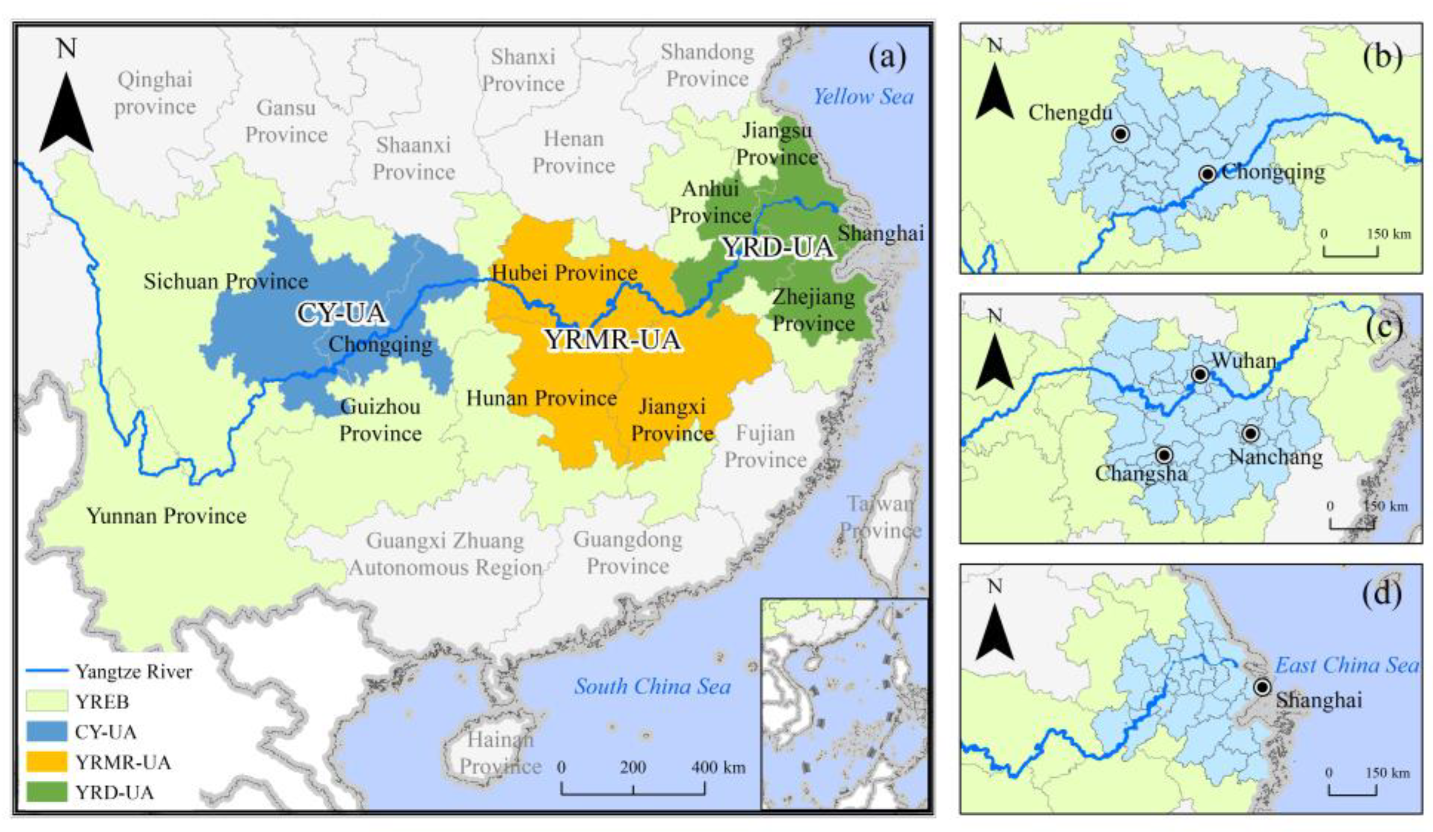
2.1. Study Area

YREB covers an area of about 205.23 × 10⁴ km² with 11 provinces and municipalities, with the population and GDP accounting for over 40% of China [27]. Since the release of the Outline of the Yangtze River Economic Belt Development Plan in September 2016, YREB has formed a development pattern of “one axis, two wings, three poles, and multiple points”. As shown in Figure 1, CY-UA, YRMR-UA, and YRD-UA are the three poles of YREB. The administrative boundary data were obtained from the Resource and Environment Science and Data Center (https://www.resdc.cn/, accessed on 2 January 2023).

Table 1. Cities in three YREB urban agglomerations.

	Cities
CY-UA	Chongqing, Chengdu, Dazhou, Deyang, Guangan, Leshan, Luzhou, Meishan, Mianyang, Nanchong, Neijiang, Suining, Yaan, Yibin, Ziyang, Zigong
YRMR-UA	Wuhan, Changsha, Nanchang, Changde, Ezhou, Fuzhou, Hengyang, Huanggang, Huangshi, Ji’an, Jingdezhen, Jingmen, Jingzhou, Jiujiang, Loudi, Pingxiang, Qianjiang, Shangrao, Tianmen, Xiantao, Xianning, Xiangtan, Xiangyang, Xiaogan, Xinyu, Yichang, Yichun, Yingtan, Yiyang, Yueyang, Zhuzhou
YRD-UA	Shanghai, Nanjing, Hangzhou, Anqing, Changzhou, Chizhou, Chuzhou, Hefei, Huzhou, Jiaxing, Jinhua, Ma’anshan, Nantong, Ningbo, Shaoxing, Suzhou, Taizhou, Taizhou, Tongling, Wuhu, Wuxi, Xuancheng, Yancheng, Yangzhou, Zhenjiang, Zhoushan

lists the cities contained in three urban agglomerations.

2.2. Datasets

2.2.1. CO₂ Emissions Data

CO₂ emissions data were obtained from the Multi-resolution Emission Inventory model for Climate and air pollution research (MEIC), which is a bottom-up multi-scale emission inventory model developed by Tsinghua University [28,29]. MEIC aims to build a high-resolution global-scale, multi-scale anthropogenic source greenhouse gas and air pollutant emission inventory model. The MEIC CO₂ emissions data at a 0.25-degree grid resolution contains industry sources, power sources, residential sources, and transportation sources (http://meicmodel.org.cn/, accessed on 29 May 2023). Based on China’s measured emission factors, MEIC is more suitable than the IPCC method for the assessment of China’s CO₂ emissions [30]. Meanwhile, MEIC has the advantages of objectivity, stability, high precision, and wide coverage and provides multi-year, different spatial scales, dynamic, and continuous CO₂ emissions monitoring information.

2.2.2. Socio-Economic Data

Based on numerous previous studies on CO₂ emissions from urban agglomerations [31,32,33], population (POP), GDP per capita (GDPPC), the proportion of secondary industry (SI), carbon emission intensity (CI), and urbanization (UR) were selected as the influencing factors of CO₂ emissions in this study. All data were derived from the China City Statistical Yearbook (2009–2018 editions).

Table 2. Brief description of influencing factors.

Factor	Abbreviation	Description	Unit
CO2 emissions	CE	Total anthropogenic CO2 emissions	104 tons
Population	POP	Total resident population	person
GDP per capita	GDPPC	GDP/Population	104 yuan/person
Proportion of secondary industry	SI	Added value of the secondary industry/GDP	%
Carbon emission intensity	CI	CO2 emissions/GDP	ton/104 yuan
Urbanization	UR	Non-agricultural population/Population	%

reports the influencing factors used in this study. POP represents the size of the population. GDPPC is the ratio of GDP to total population, which represents the regional economic development level. SI is the ratio of the value added of the secondary industry’s GDP to total GDP, which represents the industrial structure. The resource endowments in the upper, middle, and lower reaches of YREB are unbalanced, and the industrial structure differs greatly [34]. CI is the ratio of total CO₂ emissions to GDP, which represents the technology level. UR represents the urbanization level.

POP, GDPPC, SI, CI, and UR were used to construct the MGWR model to analyze the influencing factors of CO₂ emissions in YREB urban agglomerations. Moreover, GDPPC was used in EKCs to depict economic growth.

2.3. Spatial Autocorrelation

2.3.1. Global Autocorrelation

Global Moran’s I is a typical spatial autocorrelation index that measures the degree of spatial autocorrelation of CO₂ emissions in each urban agglomeration [35]. It determines whether the geographic phenomenon is aggregated. The calculation formula is as follows:

$$I=\frac{n{\sum }_{i=1}^n{\sum }_{j=1}^n{W}_{ij}\left(x_i-\overline{y}\right)\left(x_j-\overline{x}\right)}{\left({\sum }_{i=1}^n{\sum }_{j=1}^n{W}_{ij}\right){\sum }_{j=1}^n{\left(x_i-\overline{x}\right)}^2}$$

(1)

where $n$ is the number of units in each urban agglomeration, $x_i$ and $x_j$ denote the CO₂ emissions of spatial units $i$ and $j$, respectively, $\overline{x}$ denotes the average CO₂ emissions of each urban agglomeration, and $W_{ij}$ denotes the spatial weight matrix.

The value of $I$ ranges from −1 to 1. $I$ > 0 indicates positive spatial autocorrelation, and the observations tend to be spatially clustered. The closer $I$ is to 1, the stronger the aggregation. $I$ < 0 indicates negative spatial autocorrelation, and the observations tend to be dispersed. The closer $I$ is to −1, the more dispersed it is. $I$ = 0 indicates that there is no spatial autocorrelation, and the observations are randomly distributed.

2.3.2. Local Autocorrelation

The local indicators of spatial association (LISA) are used to describe the correlation between a spatial unit and its neighboring unit [36], and the formula is as follows:

$$I_i=\frac{\left(x_i-\overline{x}\right)}{S^2}\sum _{j=1}^m{W}_{ij}\left(x_j-\overline{x}\right),S^2=\frac{1}{n}\sum _{i=1}^n{\left(x_i-{\overline{x}}_i\right)}^2$$

(2)

where $x_i$ and $x_j$ denote the CO₂ emissions of spatial units $i$ and $j$, respectively, $\overline{x}$ denotes the average CO₂ emissions of the urban agglomeration, $S^2$ denotes the variance of CO₂ emissions of spatial units, $W_{ij}$ denotes the spatial weight matrix, $n$ denotes the number of spatial units in the urban agglomeration, and $m$ denotes the number of neighboring units of unit $i$.

$I_i$ > 0 means that the observations of this spatial unit and its neighboring units show a positive correlation, as high values are surrounded by high values (H-H), or low values are surrounded by low values (L-L). $I_i$ < 0 shows a negative correlation, as high values are surrounded by low values (H-L), or low values are surrounded by high values (L-H).

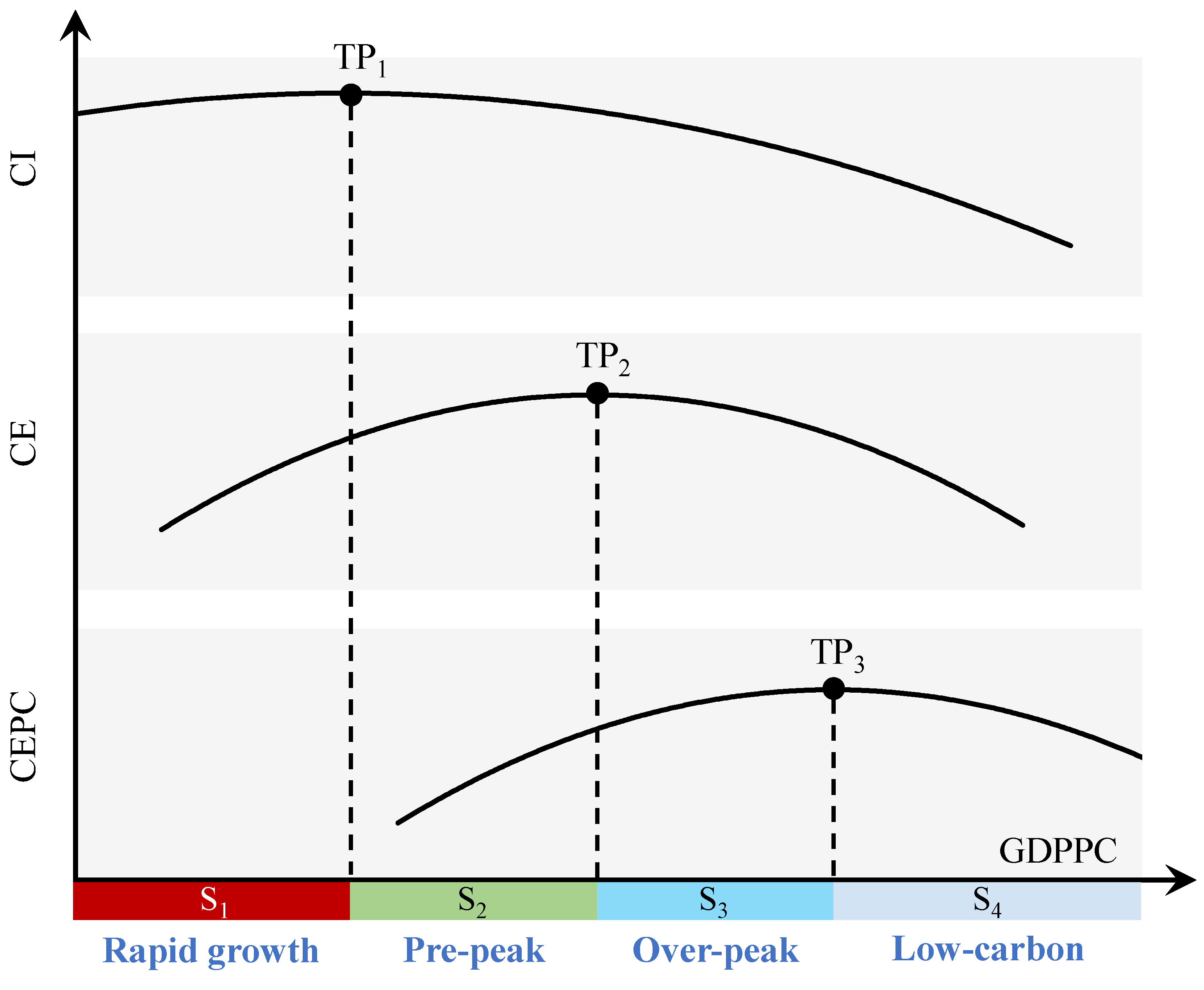
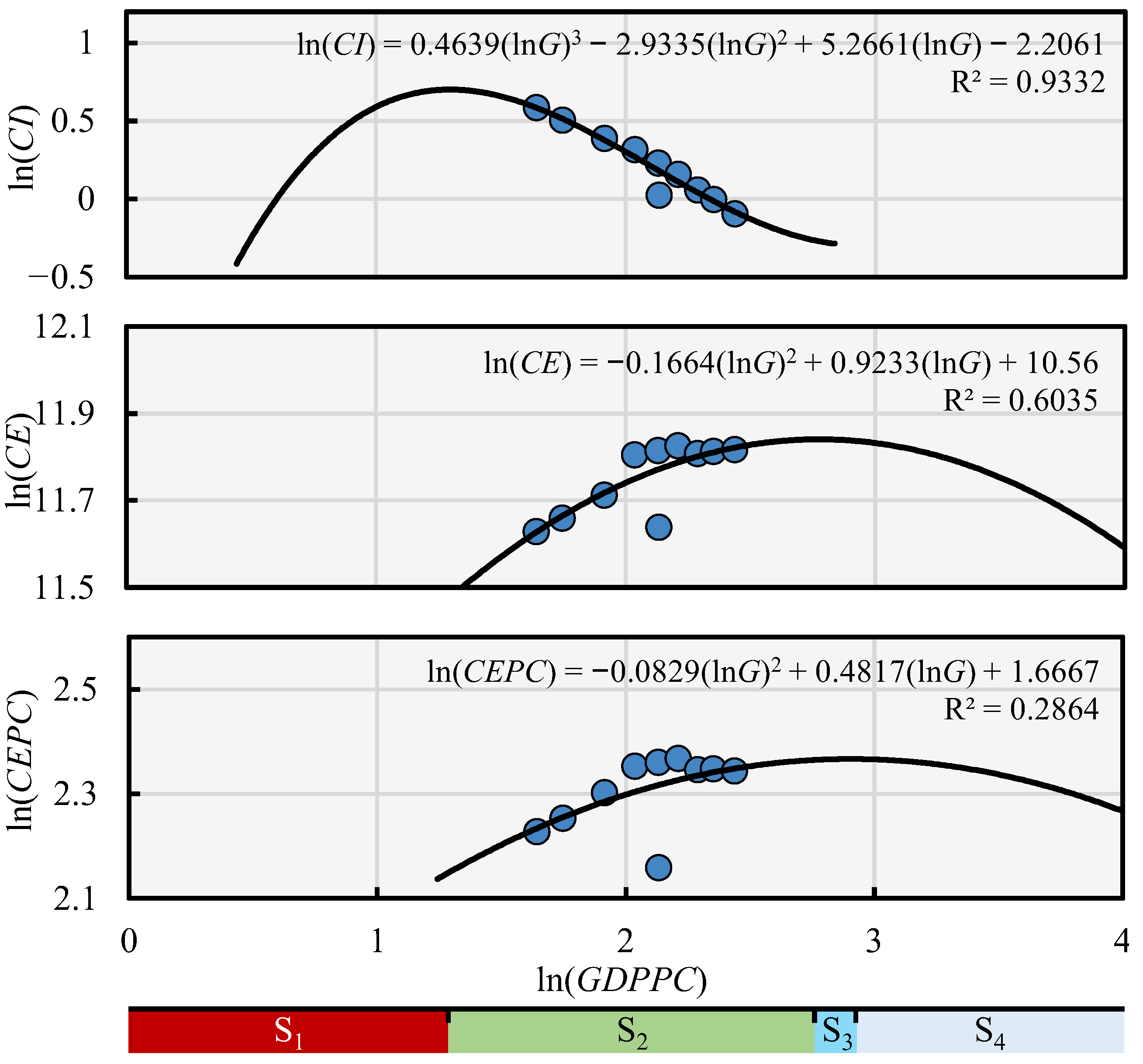
2.4. Carbon Emission Development Stage

2.4.1. Environmental Kuznets Curve (EKC)

EKC depicts the inverted U-shaped relationship between economic growth and carbon emissions [37]. In this paper, CI, CO₂ emissions per capita (CEPC), and CE are selected as indicators of carbon emissions. Meanwhile, GDPPC is used as an economic growth indicator. In this study, the quadratic polynomial is used to represent EKC, and if the coefficients of the cubic term were not significant, the quadratic polynomial is used to represent EKC [38].

$$\ln \left(E\right)={\beta }_0+{\beta }_1\left(\ln G\right)+{\beta }_2{\left(\ln G\right)}^2+{\beta }_3{\left(\ln G\right)}^3+\epsilon$$

(3)

where $E$ denotes carbon emission index, ${\beta }_0$ is a constant term, $\ln G$ denotes the natural logarithm of GDPPC, ${\beta }_1$, ${\beta }_2$, and ${\beta }_3$ are the primary, secondary, and tertiary coefficients, respectively, and $\epsilon$ is the error term.

2.4.2. Carbon Emission Development Stage Division Based on EKCs

Urban agglomerations exhibit different carbon emission characteristics at different stages of economic development. It is necessary to consider the development stage of carbon emissions with the state of economic development. As shown in Figure 2, there are three types of EKCs that present a relationship between carbon emissions and economic growth [39]: (1) EKC with CI, where GDPPC is the independent variable and CI is the dependent variable; (2) EKC with CE, where GDPPC is the independent variable and CE is the dependent variable; and (3) EKC with CEPC, where GDPPC is the independent variable and CEPC is the dependent variable. There is a turning point for each curve, namely TP₁, TP₂, and TP₃. The development stage of carbon emissions can be divided into four stages based on the three TPs of the EKCs. S₁ is the rapid growth stage, where the carbon emission index increases rapidly with economic growth; S₂ is the pre-peak stage, where the carbon emission index continues to grow but at a slower rate and decreases until it reaches the peak; and S₃ is the over-peak stage, in which the carbon emission index starts to decrease. S₄ is the low-carbon stage, in which the carbon emission index gradually decreases to a lower level.

2.5. MGWR Model

MGWR is an extension of geographic weighted regression (GWR) and has been widely used in the analysis of spatial relationships of explanatory variables. GWR is a model for geographic analysis that allows the model parameters to be verified based on a specific location [40]. The GWR model is formulated as follows:

$$y_i={\beta }_0\left(u_i,v_i\right)+\sum _{j=1}^n{\beta }_j\left(u_i,v_i\right)x_{ij}+{\epsilon }_i$$

(4)

where $i$ represents the $i$-th unit, $\left(u_i,v_i\right)$ are the latitude and longitude coordinates of city $i$, $y_i$ is the CO₂ emissions of unit $i$, ${\beta }_0\left(u_i,v_i\right)$ is the intercept at $i$, ${\beta }_j\left(u_i,v_i\right)$ is the regression coefficient of the $j$-th variable of unit $i$, $j$ denotes the uniform bandwidth of the regression coefficient, $x_{ij}$ is the $j$-th influencing factor for unit $i$, and $\epsilon$ is the error term of $i$. When ${\beta }_j\left(u_i,v_i\right)$ is a constant, GWR is equal to the ordinary least squares (OLS) model.

However, the bandwidth of GWR is constant, and it cannot explain the phenomena, which involve numerous spatial processes with various [41]. Therefore, Fotheringham et al. (2017) proposed a multiscale geographically weighted regression (MGWR) model [42]. MGWR allows an optimal bandwidth for the explanatory variables based on local regression. MGWR is formulated as follows:

$$y_i={\beta }_{bw0}\left(u_i,v_i\right)+\sum _{j=1}^n{\beta }_{bwj}\left(u_i,vi\right)x_{ij}+{\epsilon }_i$$

(5)

where $bw0$ denotes the bandwidth used for the regression coefficient of the global variable, $bwj$ denotes the bandwidth used for the regression coefficient of the $j$-th variable, and the other variables have the same meaning as in the GWR model.

3. Results

3.1. Spatiotemporal Variation of CO₂ Emissions

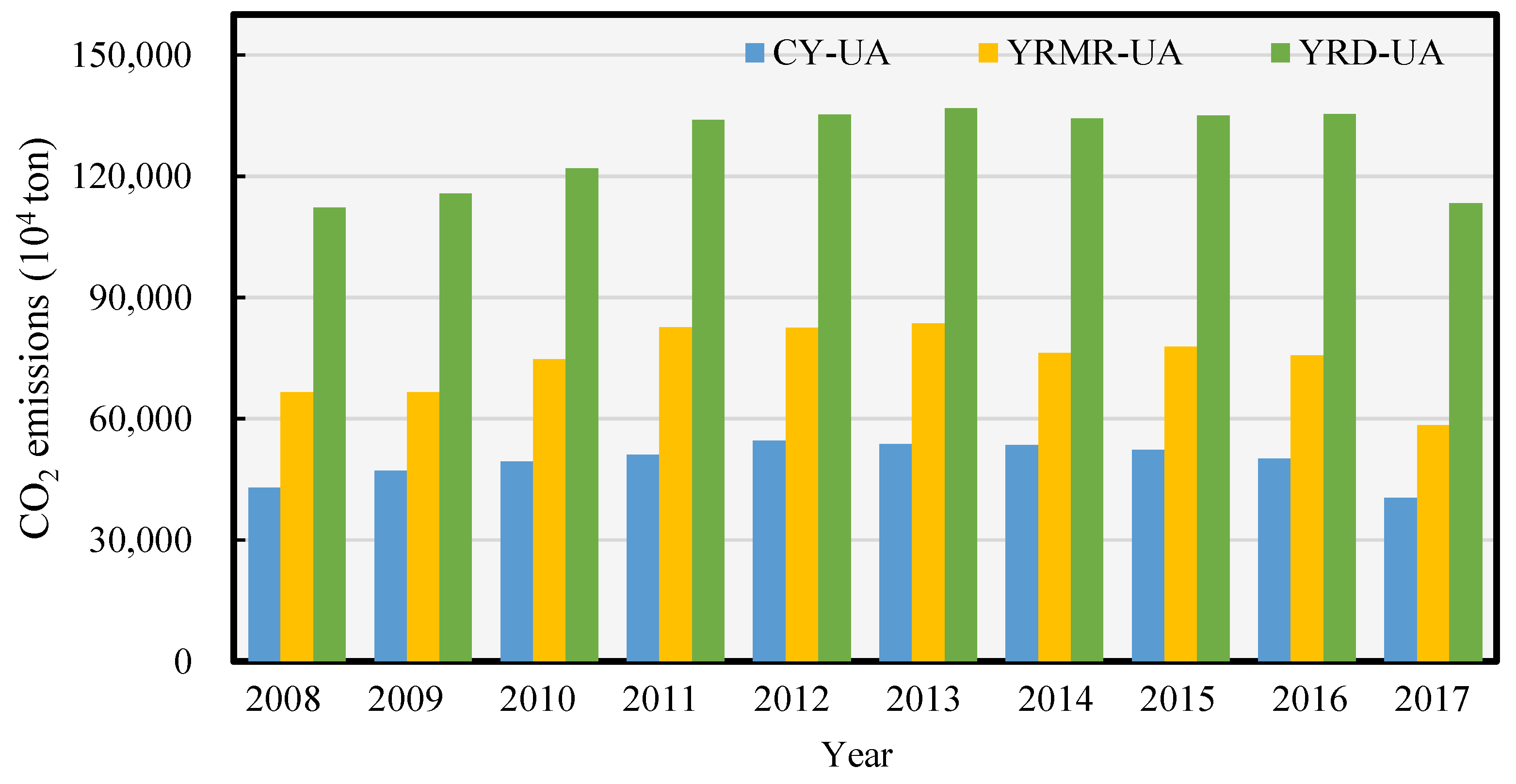
3.1.1. Temporal Variation of CO₂ Emissions

Figure 3 shows the CO₂ emissions of three urban agglomerations in YREB during 2008–2017. The CO₂ emissions of three urban agglomerations reached their peak around 2012–2013 and then began to decrease, with the lowest emissions of the three urban agglomerations in 2017. Moreover, the CO₂ emissions of YRD-UA were much higher than those of CY-UA and YRMR-UA, where 41.87% of the CO₂ emissions in YREB were contributed by YRD-UA. YRD-UA had entered the middle and late stages of urban agglomeration development with a higher level of regional integration and stronger comprehensive strength [43]. The CO₂ emissions of CY-UA were the lowest among the urban agglomerations since CY-UA was at the initial stage of urban agglomeration development with fewer megacities [44].

Since 2013, the CO₂ emissions of three YREB urban agglomerations have shown a decreasing trend; CY-UA reached its peak around 2012, while YRMR-UA and YRD-UA reached their peaks around 2013. Specifically, the CO₂ emissions in YRMR-UA declined most significantly, while the CO₂ emissions decline in YRD-UA was relatively stable. In 2016, a symposium on comprehensively advancing the development of the sustainable development of YREB was held for the first time, highlighting the importance of ecological conservation and environmental management [45]. The significant reduction of CO₂ emissions in 2017 illustrated the effectiveness of government policies.

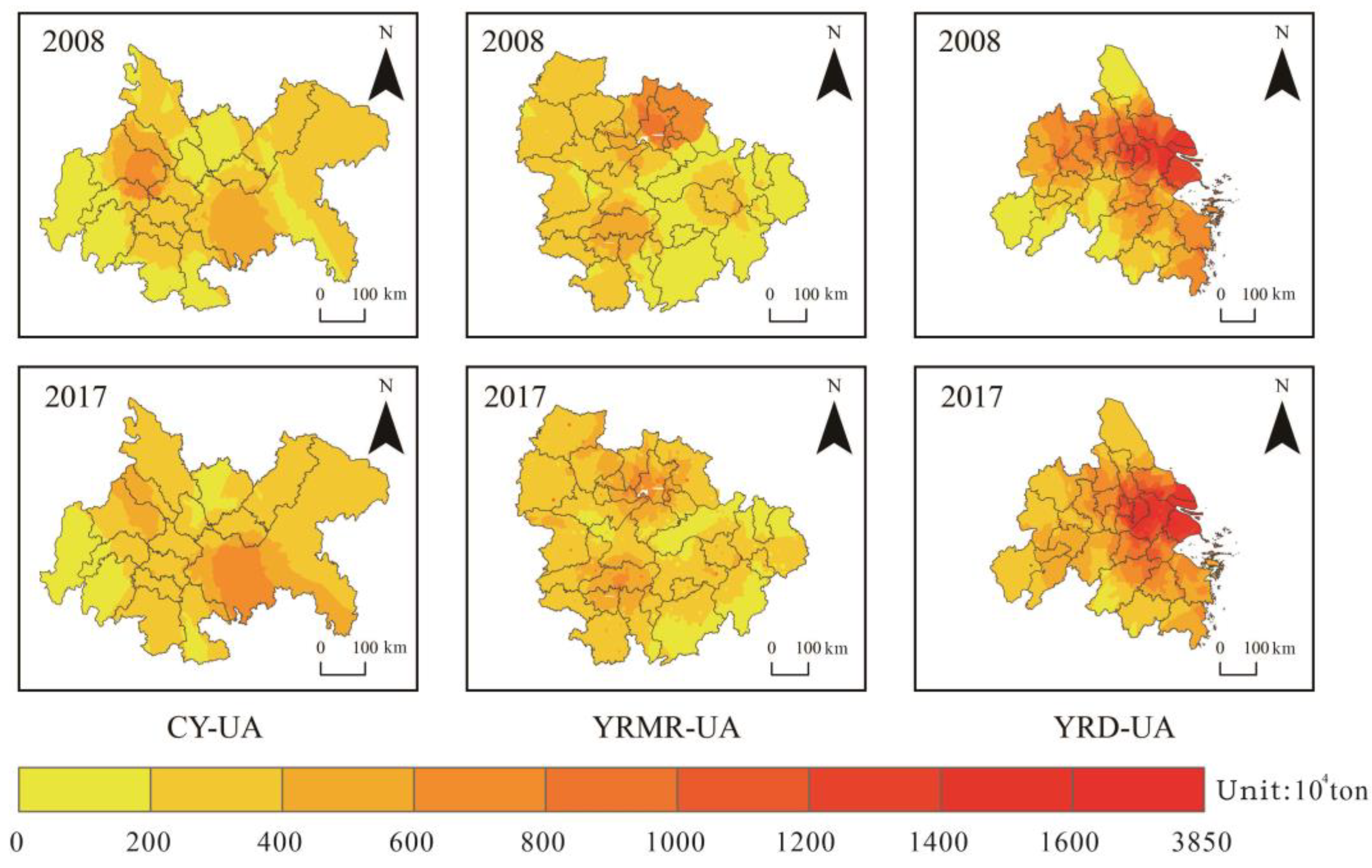
3.1.2. Spatial Variation of CO₂ Emissions

Figure 4 shows the CO₂ emissions in 2008 and 2017. The 10-year average CO₂ emissions of CY-UA was 49,553 × 10⁴ tons, with the low-value area distributed in the western mountainous area and northern mountainous areas, and the high-value area distributed in the urban areas around Chongqing and Chengdu. The 10-year average CO₂ emissions of YRMR-UA was 74,461 × 10⁴ tons, with the low-value area distributed in the southern mountainous area and the border of Jiangxi and Hubei provinces, and the high-value area distributed in Wuhan, Changsha, and Nanchang. For YRD-UA, the 10-year average CO₂ emissions was 127,413 × 10⁴ tons, with the low-value areas distributed in the southwestern mountains and western and northern plains, and the high-value areas distributed in Shanghai, Hangzhou, Nanjing, and the surrounding areas. Notably, the CO₂ emissions of several large cities, such as Chengdu in the CY-UA and Wuhan in the YRMR-UA, decreased in 2017 compared to 2008.

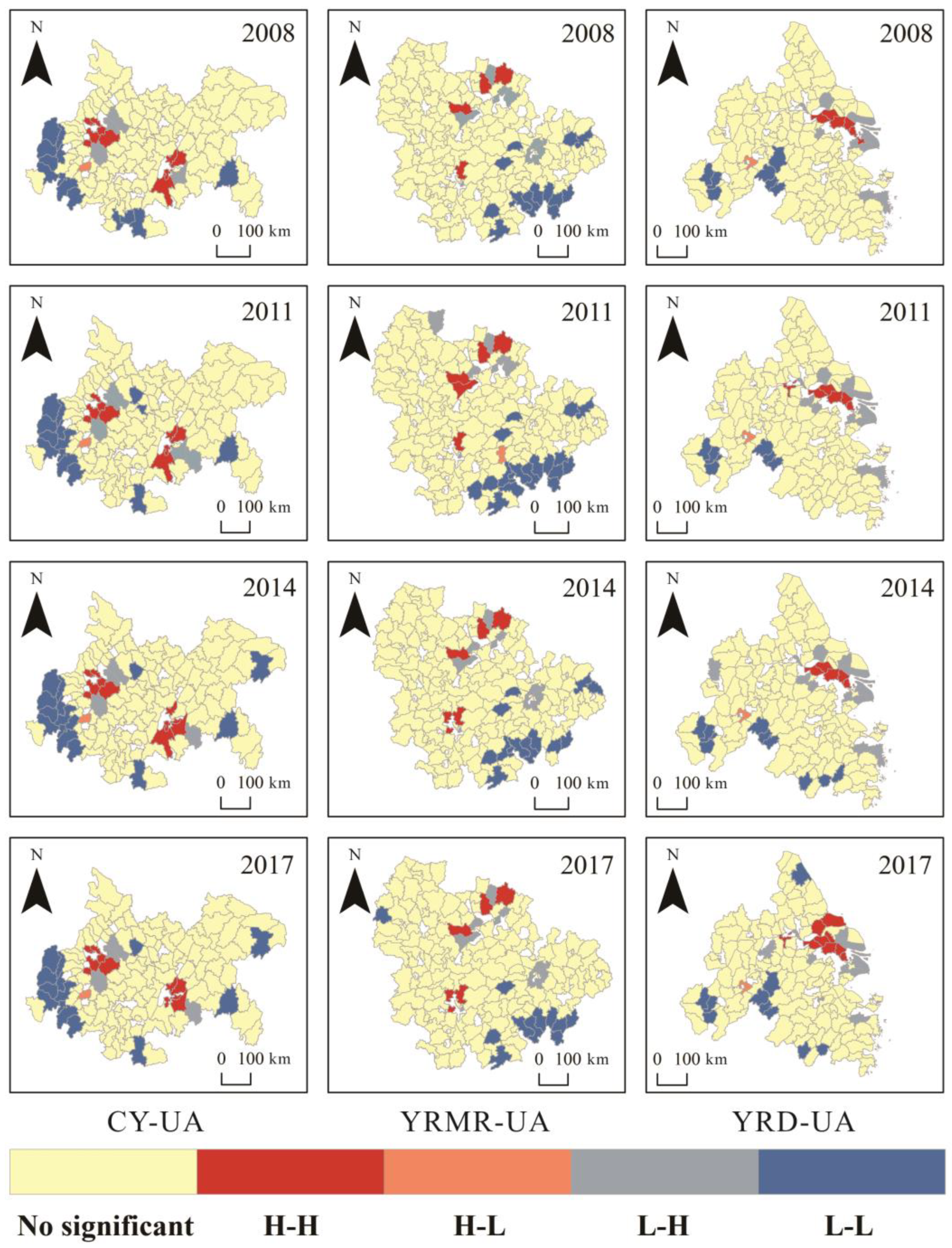
3.1.3. Spatial Aggregation of CO₂ Emissions

Table 3. Global spatial autocorrelation of CO₂ emissions in three urban agglomerations.

2008	CY-UA	YRMR-UA	YRD-UA	2017	CY-UA	YRMR-UA	YRD-UA
Moran’s I	0.146	0.034	0.180	Moran’s I	0.173	0.045	0.135
Z score	4.260	0.969	3.257	Z score	5.463	1.105	2.427
p value	0.000	0.333	0.001	p value	0.000	0.269	0.015

shows the global autocorrelation performance. The Z score is a multiple of the standard deviation, and the p value indicates probability. Z is correlated with p, where p < 0.05 indicates that the confidence level is greater than 95% [46]. CY-UA and YRD-UA presented significant spatial aggregation characteristics. The Moran’s I of CY-UA in 2008 and 2017 were 0.146 and 0.173, respectively, where the spatial autocorrelation of CO₂ emissions increased. The Moran’s I of YRMR-UA in 2008 and 2017 was 0.034 and 0.045, respectively. As for YRD-UA, the Moran’s I was 0.180 and 0.135 in 2008 and 2017, respectively.

Figure 5 shows the spatial aggregation characteristics of the CO₂ emissions of three urban agglomerations. For CY-UA, the H-H clusters and L-H clusters were distributed around Chongqing and Chengdu, and the L-L clusters were distributed in the western mountainous areas and scattered in the south and east. The cluster pattern of CO₂ emissions in CY-UA can be described as high in the middle and low around, and the overall pattern has not changed in the decade. For YRMR-UA, the H-H clusters mainly appeared in the north area, the L-H clusters mainly appeared around Wuhan, Changsha, and Nanchang, and the L-L clusters appeared in the southeast area. The cluster pattern of CO₂ emissions in YRMR-UA was high in the north and low in the south. For YRD-UA, the H-H clusters and L-H clusters were mainly distributed in the eastern coastal area, including Shanghai and Nanjing, while the L-L clusters were scattered in the south and southwest areas. The cluster pattern of CO₂ emissions in YRD-UA was high along the coast and low in the southwest.

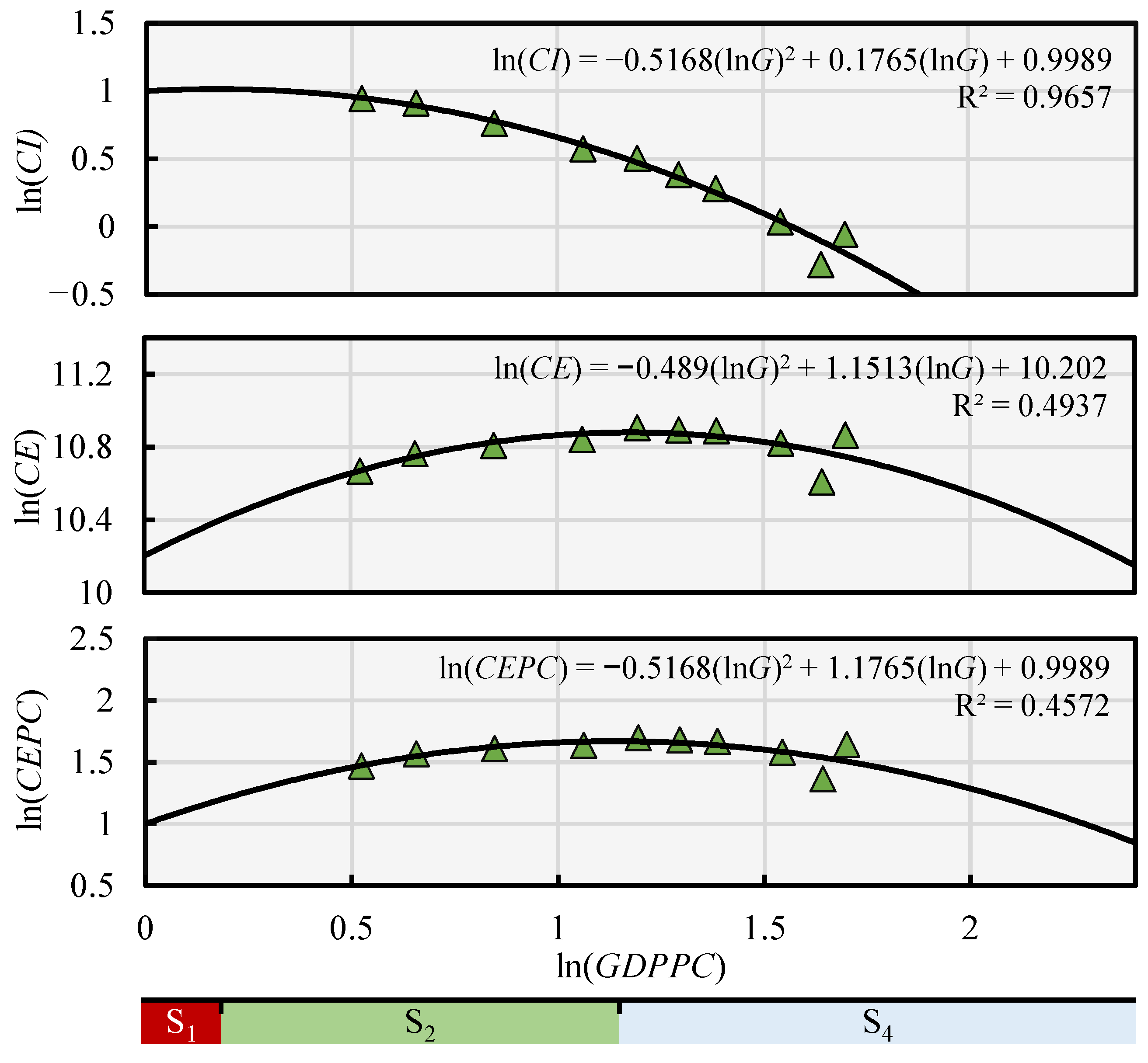
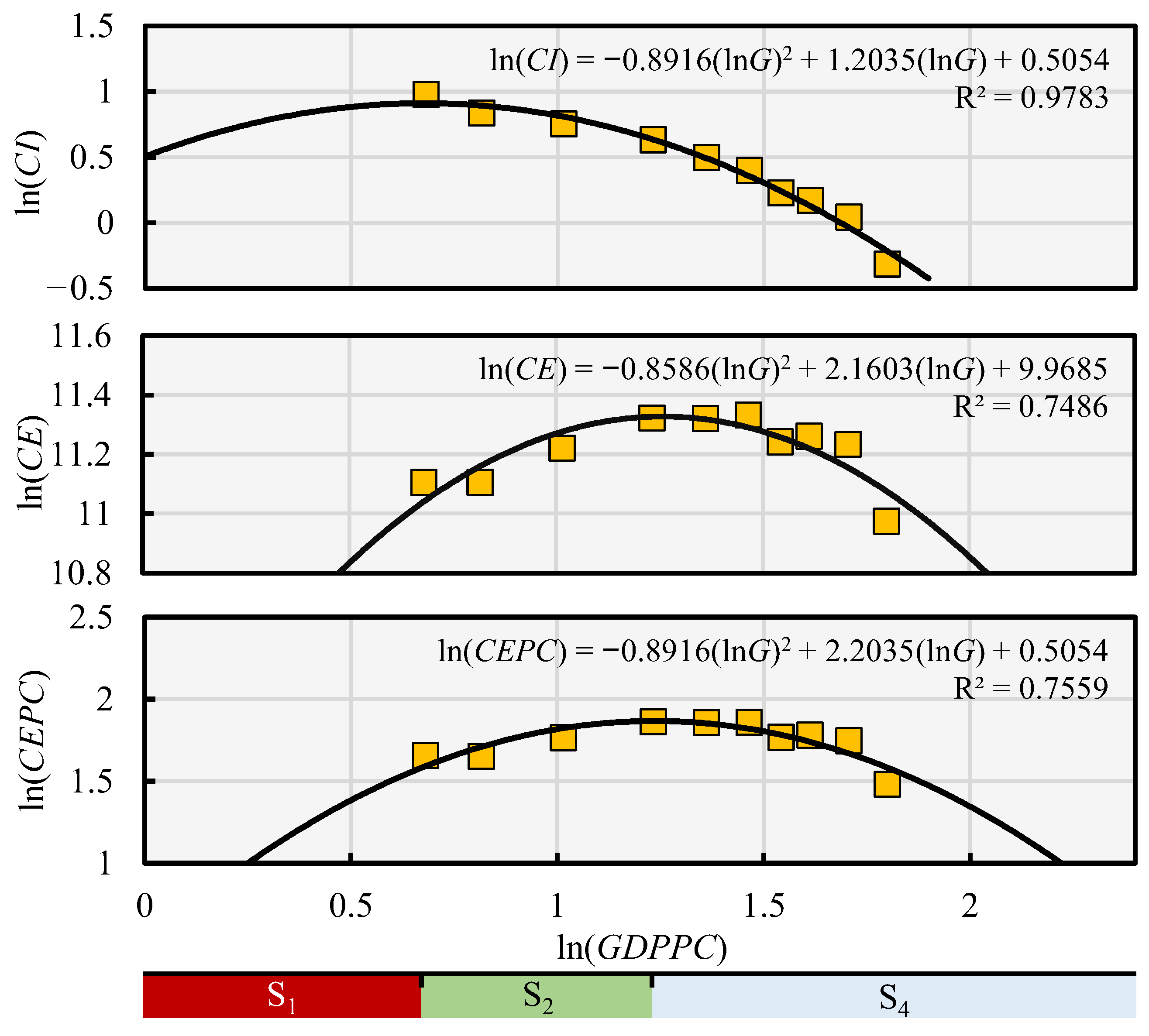
3.2. Carbon Emission Development Stage Analysis

Figure 6 shows the relationship between carbon emissions and GDPPC for CY-UA. The carbon emission development stage of CY-UA could be divided into three stages: S₁ (–2005), S₂ (2005–2012), and S₄ (2012–). S₃ and S₄ of CY-UA largely overlapped and could be combined into one stage. The peak time of CO₂ emissions in CY-UA was around 2011, and CY-UA is at the low-carbon stage.

Figure 7 shows the relationship between carbon emissions and GDPPC for YRMR-UA. Similar to CY-UA, the S₃ and S₄ stages of YRMR-UA were combined. The YRMR-UA CO₂ emissions could be divided into three stages: S₁ (–2008), S₂ (2008–2011), and S₄ (2011–). The peak time of CO₂ emissions in YRMR-UA was around 2011, and YRMR-UA is at the low-carbon stage.

Figure 8 shows the relationship between carbon emissions and GDPPC for YRD-UA. The emissions of YRD-UA could be divided into four stages: S₁ (–2005), S₂ (2005–2020), S₃ (2020–2022), and S₄ (2022–). The CO₂ emissions of YRD-UA reached the peak around 2020, and YRD-UA was at S₄ stage. Obviously, the actual CO₂ emissions peaked earlier than the carbon emission development stage. It could be concluded that the Yangtze River Delta integration policy strongly deepened the industrial division of labor and industrial transfer among cities, which contribute to the reduction of CO₂ emissions.

3.3. Model Comparison

3.3.1. Comparison of Model Performance

Table 4. Comparison of OLS, GWR, and MGWR indicators from 2008–2017.

Year	Model	R2	Adjusted R2	AICc	RSS	ENP
2008	MGWR	0.96	0.95	5.38	2.85	11.42
	GWR	0.96	0.95	7.40	2.80	12.52
	OLS	0.93	0.92	1159.39	/	/
2011	MGWR	0.95	0.94	13.24	3.33	10.42
	GWR	0.95	0.94	17.48	3.81	8.61
	OLS	0.93	0.92	1177.63	/	/
2014	MGWR	0.95	0.94	12.45	3.35	10.01
	GWR	0.95	0.94	13.92	3.59	8.83
	OLS	0.93	0.93	1165.29	/	/
2017	MGWR	0.88	0.87	74.08	8.12	9.88
	GWR	0.87	0.86	75.64	8.80	8.43
	OLS	0.86	0.85	1204.20	/	/

shows the statistical results of OLS, GWR, and MGWR. R² is the coefficient of determination. Adjusted R² excludes the effect of the number of independent variables on R². AICc denotes the corrected Akaike information criterion, which is a relative measure of the goodness of fit [47]. RSS is the sum of squared errors. The effective number of parties (ENP) is a trade-off between the variance of the fitted values and the deviation of the coefficient estimates to measure the value of the equilibrium point.

As shown in Table 4, compared to GWR and OLS, MGWR gave higher R², adjusted R², and ENP, with lower AICc and RSS, indicating that MGWR had a better local fit and less information loss. Meanwhile, the spatial distribution of R² for GWR and MGWR is presented in Figure 9. CY-UA shows a higher R² than the other urban agglomerations.

3.3.2. Comparison of Model Bandwidth

Table 5. Bandwidths of different influencing factors in MGWR and GWR.

Factors	2008		2011		2014		2017
	MGWR	GWR	MGWR	GWR	MGWR	GWR	MGWR	GWR
POP	66	51	68	67	68	66	68	69
GDPPC	48	51	59	67	53	66	68	69
SI	68	51	68	67	68	66	68	69
CI	44	51	48	67	68	66	52	69
UR	46	51	46	67	46	66	44	69

presents the bandwidths of each influencing factor for GWR and MGWR in different years. In GWR, the factors shared the same bandwidth, while they were assigned to different bandwidths in MGWR. The different values of bandwidth demonstrated the spatial heterogeneity of factors, by which the diversity of influencing factors can be better represented [48].

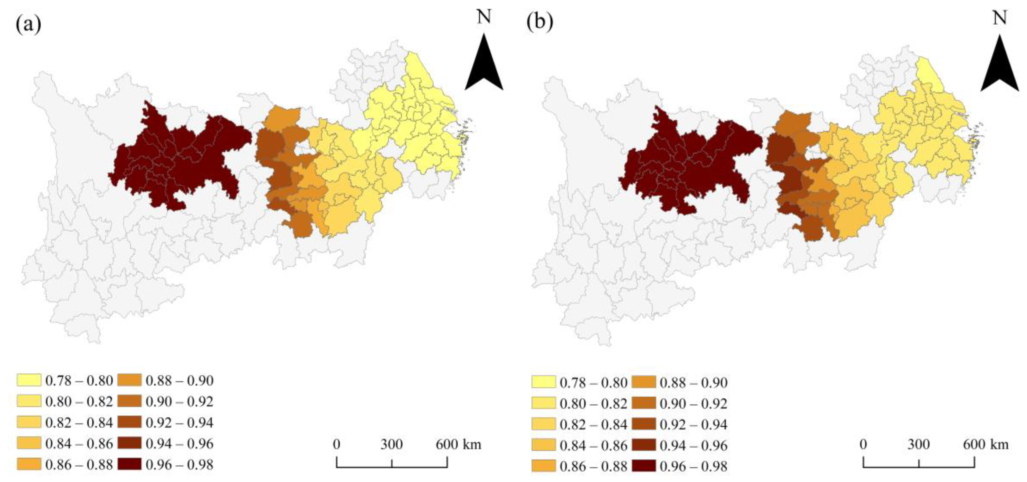
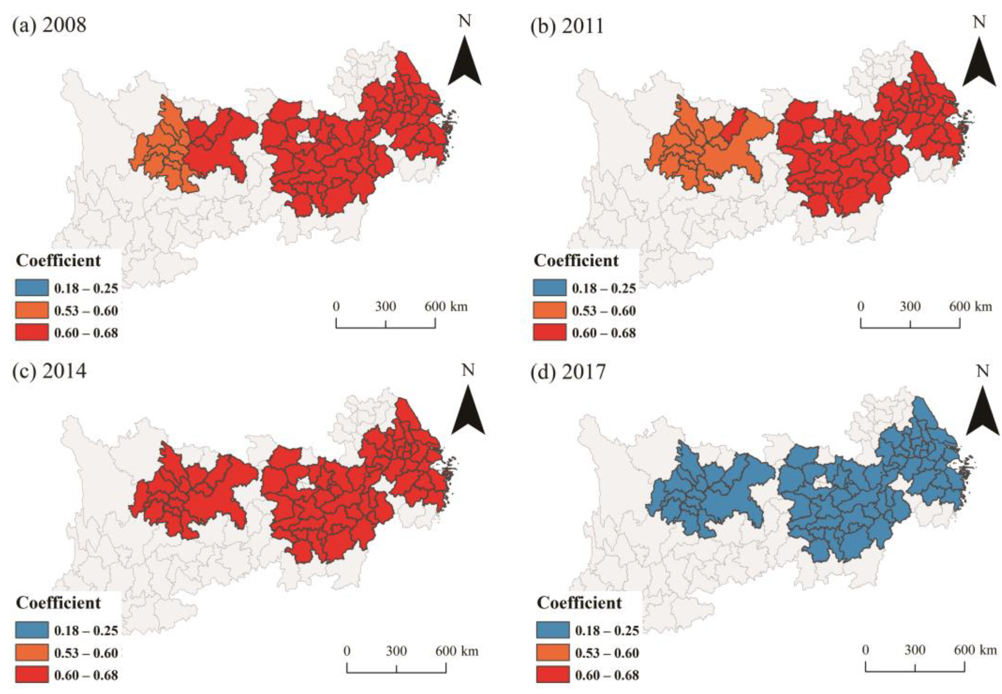
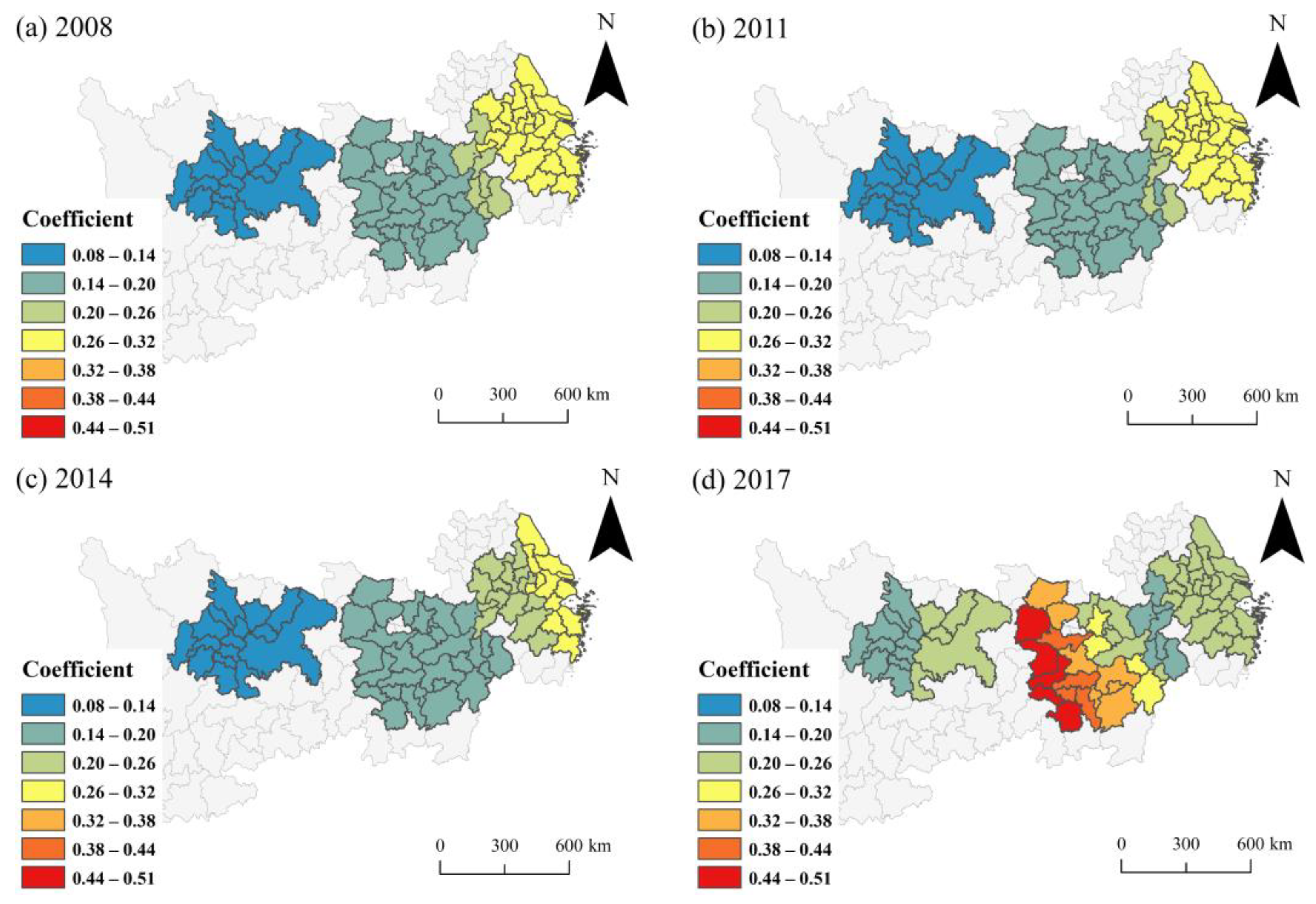
3.4. Influencing Factors for CO₂ Emissions

Table 6. Statistics of regression coefficients for different influencing factors in MGWR.

Factors	Year	Min	Median	Max	Mean	STD
POP	2008	0.637	0.818	0.992	0.814	0.134
	2011	0.664	0.814	0.89	0.79	0.089
	2014	0.705	0.805	0.961	0.821	0.102
	2017	0.719	0.732	0.743	0.733	0.007
GDPPC	2008	0.594	0.659	0.678	0.647	0.03
	2011	0.591	0.63	0.647	0.625	0.019
	2014	0.635	0.647	0.66	0.65	0.007
	2017	0.183	0.192	0.234	0.201	0.018
SI	2008	−0.034	−0.017	0.106	0.011	0.052
	2011	−0.035	−0.027	0.011	−0.019	0.017
	2014	0.016	0.022	0.047	0.028	0.012
	2017	0.037	0.065	0.083	0.063	0.015
CI	2008	0.098	0.184	0.285	0.202	0.066
	2011	0.105	0.171	0.3	0.195	0.066
	2014	0.082	0.16	0.269	0.177	0.063
	2017	0.157	0.236	0.509	0.262	0.091
UR	2008	−0.068	0.075	0.161	0.041	0.07
	2011	−0.038	0.038	0.111	0.027	0.038
	2014	−0.048	−0.044	−0.004	−0.033	0.017
	2017	0.132	0.214	0.408	0.255	0.108

shows the descriptive statistics of the regression coefficients of influencing factors in MGWR. It can be seen that the rank of the generated regression coefficients was POP > GDPPC > CI > UR > SI. Obviously, POP and GDPPC presented the highest regression coefficients. The coefficient of POP is positive, indicating that the rise of population will promote the CO₂ emissions of urban agglomerations in YREB. GDPPC presented the second highest regression coefficient, indicating that GDPPC had a facilitating effect on CO₂ emissions. The coefficients of UR and SI were much lower, and their impact on CO₂ emissions was not significant.

Figure 10 shows the spatial distribution of the regression coefficients of POP. There was a significant positive correlation between POP and CE, where an increase in population will increase energy consumption and thus produce more CO₂ emissions [49]. The impact of POP on CE was significant in YRD-UA. YRD-UA was an important economic center in China, which provided sufficient jobs and attracted a large number of migrants [50]. Traffic congestion caused by population concentration was not conducive to adequate combustion of fuels [51], leading to an increase in transportation CO₂ emissions. The transportation CO₂ emissions in YRD-UA amounted to 9971.78 × 10⁴ tons in 2017, which is approximately equal to the sum of CY-UA and YRMR-UA.

Figure 11 shows the spatial distribution of regression coefficients for GDPPC. The positive correlation between GDPPC and CE indicates that the growth of GDPPC promoted CO₂ emissions in YREB urban agglomerations. The influence of GDPPC on CE was significant in YRD-UA, and the regression coefficient decreased from east to west in 2008, 2011, and 2014. Economically developed regions responded better to the policy. The government improves local competitiveness in response to economic conditions [52]. More attention should be paid to the change in people’s awareness and environmental management caused by the economic improvement.

Figure 12 shows the spatial distribution of the regression coefficients of CI. The positive correlation between CI and CE indicates that the adoption of technological innovations and the improvement of energy use efficiency reduced CO₂ emissions [53]. The impact of CI on CE was significant in YRD-UA. Technological advances promoted the harmonization of economic and environmental development [54]. Companies were more inclined to use environmentally friendly technologies [55].

Figure 13 shows the spatial distribution of regression coefficients for UR. The impact of UR on CE was insignificant, and the value of the regression coefficient varied between −0.07 and 0.41. The reason was that urbanization led to an increase in people’s demand for employment, housing, transportation, commodities, and energy dependence [56], and urban construction increased society’s demand for high-emitting industries such as steel and cement [57].

Figure 14 shows the spatial distribution of regression coefficients for SI. SI presented a negative correlation with CE in 2008 and 2011, while SI positively correlated with CE in 2014 and 2017. The reason may be that some cities in YREB were at the stage of industrial start-up and development. YRD-UA was dominated by light industry and high-tech industry with low CO₂ emissions [58]. YRMR-UA was at the initial stage of the Rise of Central China Plan, and CY-UA was vital to China’s western development [59]. The industrial layout and energy structure of YREB are gradually maturing.

It is noteworthy that the spatial distribution of five influencing factors changed significantly in 2017. The spatial heterogeneity of POP decreased, the impact of GDPPC decreased, the spatial heterogeneity of CI increased, and the spatial heterogeneity of UR increased. It may be due to the convening of the symposium on comprehensively advancing the development of sustainable development in YREB held in 2016. The difference in the sensitivities of inland and coastal cities to policies resulted in changes in the regression coefficients of the influencing factors in 2017.

4. Discussion

4.1. Insights into the CO₂ Emissions of YREB Urban Agglomerations

As a pioneer demonstration belt for the construction of ecological civilization in China, YREB is of great significance to China and the world in achieving emission reduction and sustainable development. Different urban agglomerations present different carbon emission characteristics at different stages of economic development, making it important to develop targeted emission reduction measures. China is in the process of rapid urbanization and industrialization [60]. In 2017, the proportion of tertiary industry in YRD-UA was 2.84% higher than the proportion of secondary industry [53]. Several cities in the southeast coastal region had already crossed the industrialization stage and entered the post-industrialization period [61], which was confirmed by the low proportion of industrial CO₂ emissions in YRD-UA and the significant growth of electricity CO₂ emissions. However, most cities in central and western China were in the process of industrialization, and the proportion of tertiary industry was lower than the proportion of secondary industry [62], which led to a higher proportion of industrial CO₂ emissions in CY-UA and YRMR-UA than that in YRD-UA.

The optimization and upgrading of industrial structures could promote carbon mitigation in CY-UA and YRMR-UA. Specifically, attention can be paid to industries such as electronic information, engineering machinery, rail transportation equipment, automobiles, aerospace, biomedicine, and new materials. In addition, CY-UA and YRMR-UA could undertake the transfer of high-tech industries from the developed coastal regions. With the deepening of the 14th Five-Year Plan and the vigorous development of wind, hydro, and photovoltaic power generation [63], renewable energy will be the mainstream of the future energy structure in YREB. The west-east gas pipeline project has provided cleaner energy and reduced fossil fuel consumption [64]. More attention should be paid to taking measures to reduce CO₂ emissions from production and life while increasing the share of the service industry in the regional economy. Meanwhile, YRD-UA should focus on reducing the facilitating effects of population on CO₂ emissions by considering human capital agglomeration in the process of urbanization [65]. The investigation of spatiotemporal variations in CO₂ emissions contributes to timely policy adjustments for carbon emission mitigation in YREB urban agglomerations. Meanwhile, EKCs revealed the relationship between CO₂ emissions and economic development, providing a strategy that can be applied to analyze the carbon emission development stage of more regions. Furthermore, the importance of different influencing factors for CO₂ emissions was generated and discussed, which can be conducive to promoting regional sustainable development.

4.2. Limitations

This study investigated the CO₂ emissions of YREB urban agglomerations, but there is still room for further research. The MEIC CO₂ emissions data is from 2008 to 2017, and the spatiotemporal patterns of CO₂ emissions after 2017 were not explored in this study. Therefore, expanded CO₂ emissions datasets with more recent years will be considered in the future. Meanwhile, five influencing factors that reveal economic and social characteristics were selected in this study, and future studies will focus on the selection of representative and comprehensive influencing factors of CO₂ emissions in urban agglomerations.

5. Conclusions

This paper revealed the spatial and temporal variations of CO₂ emissions in three urban agglomerations in YREB. Meanwhile, the carbon emission development stage of the YREB urban agglomerations was explored based on EKCs that take economic growth and carbon emissions into account. In addition, the influencing factors of CO₂ emissions were analyzed using MGWR. The main conclusions are as follows:

(1)

The CO₂ emissions in the three urban agglomerations first increased and then decreased from 2008 to 2017. YRD-UA contributed 41.87% of the CO₂ emissions of YREB, with the highest CO₂ emissions among the three urban agglomerations. A symposium on comprehensively advancing the development of the sustainable development of YREB was held in 2016, and the CO₂ emissions in three urban agglomerations decreased significantly in 2017.

(2)

The carbon emission development stage of urban agglomeration was analyzed based on the relationship between carbon emissions and economic growth. According to the EKCs, CY-UA, YRMR-UA, and YRD-UA reached the CO₂ emissions peaks around 2012, 2011, and 2020, respectively. Nowadays, the urban agglomerations in YREB are at the low-carbon stage.

(3)

The CO₂ emissions of YREB urban agglomerations were significantly affected by POP and GDPPC, while the impacts of UR and SI were not significant. The spatial distribution of influencing factors changed significantly in 2017. To reduce CO₂ emissions, human capital agglomeration and clean energy should be considered in the process of urbanization.

Moreover, future work will focus on the long-term carbon emission development stage analysis of typical urban agglomerations, where more comprehensive CO₂ emissions data and influencing factors will be taken into account.

References

1. Clark, P.U.; Shakun, J.D.; Marcott, S.A.; Mix, A.C.; Eby, M.; Kulp, S.; Levermann, A.; Milne, G.A.; Pfister, P.L.; Santer, B.D.; et al. Consequences of twenty-first-century policy for multi-millennial climate and sea-level change. Nat. Clim. Change 2016, 6, 360–369. [Google Scholar] [CrossRef]
2. Wang, S.; Wang, J.; Li, S.; Fang, C.; Feng, K. Socioeconomic driving forces and scenario simulation of CO2 emissions for a fast-developing region in China. J. Clean. Prod. 2019, 216, 217–229. [Google Scholar] [CrossRef]
3. Lindsey, R.; Dahlman, L. Climate Change: Global Temperature. 2020. Available online: https://www.climate.gov/news-features/understanding-climate/climate-change-global-temperature (accessed on 1 January 2023).
4. Frame, D.J.; Held, H.; Kriegler, E.; Mach, K.J.; Matschoss, P.R.; Plattner, G.-K.; Zwiers, F.W.; Matschoss, P.R. Guidance Note for Lead Authors of the IPCC Fifth Assessment Report on Consistent Treatment of Uncertainties. Intergovernmental Panel on Climate Change (IPCC). Available online: http://www.ipcc.ch (accessed on 30 March 2023).
5. Qian, Y.; Wang, H.; Wu, J. Spatiotemporal association of carbon dioxide emissions in China’s urban agglomerations. J. Environ. Manage. 2022, 323, 116109. [Google Scholar] [CrossRef]
6. Wang, F.; Harindintwali, J.D.; Yuan, Z.; Wang, M.; Wang, F.; Li, S.; Yin, Z.; Huang, L.; Fu, Y.; Li, L.; et al. Technologies and perspectives for achieving carbon neutrality. Innovation 2021, 2, 100180. [Google Scholar] [CrossRef] [PubMed]
7. Dong, F.; Li, Y.; Gao, Y.; Zhu, J.; Qin, C.; Zhang, X. Energy transition and carbon neutrality: Exploring the non-linear impact of renewable energy development on carbon emission efficiency in developed countries. Resour. Conserv. Recycl. 2022, 177, 106002. [Google Scholar] [CrossRef]
8. Xiao, Y.; Ma, D.; Zhang, F.; Zhao, N.; Wang, L.; Guo, Z.; Zhang, J.; An, B.; Xiao, Y. Spatiotemporal differentiation of carbon emission efficiency and influencing factors: From the perspective of 136 countries. Sci. Total Environ. 2023, 879, 163032. [Google Scholar] [CrossRef]
9. Andreoni, V.; Galmarini, S. Drivers in CO2 emissions variation: A decomposition analysis for 33 world countries. Energy 2016, 103, 27–37. [Google Scholar] [CrossRef]
10. Grodzicki, T.; Jankiewicz, M. The impact of renewable energy and urbanization on CO2 emissions in Europe—Spatio-temporal approach. Environ. Dev. 2022, 44, 100755. [Google Scholar] [CrossRef]
11. Namahoro, J.; Wu, Q.; Zhou, N.; Xue, S. Impact of energy intensity, renewable energy, and economic growth on CO2 emissions: Evidence from Africa across regions and income levels. Renew. Sustain. Energy Rev. 2021, 147, 111233. [Google Scholar] [CrossRef]
12. Fragkias, M.; Lobo, J.; Strumsky, D.; Seto, K.C. Does size matter? Scaling of CO2 emissions and US urban areas. PLoS ONE 2013, 8, e64727. [Google Scholar] [CrossRef]
13. Wen, L.; Shao, H. Analysis of influencing factors of the CO2 emissions in China: Nonparametric additive regression approach. Sci. Total Environ. 2019, 694, 133724. [Google Scholar] [CrossRef]
14. Liu, Z.; Deng, Z.; He, G.; Wang, H.; Zhang, X.; Lin, J.; Qi, Y.; Liang, X. Challenges and opportunities for carbon neutrality in China. Nat. Rev. Earth Environ. 2021, 3, 141–155. [Google Scholar] [CrossRef]
15. Zeng, N.; Jiang, K.; Han, P.; Hausfather, Z.; Cao, J.; Kirk-Davidoff, D.; Ali, S.; Zhou, S. The Chinese carbon-neutral goal: Challenges and prospects. Adv. Atmos. Sci. 2022, 39, 1229–1238. [Google Scholar] [CrossRef] [PubMed]
16. Wang, K.; Zhang, X.; Wei, Y.-M.; Yu, S. Regional allocation of CO2 emissions allowance over provinces in China by 2020. Energy Policy 2013, 54, 214–229. [Google Scholar] [CrossRef]
17. Liu, J.; Tian, Y.; Huang, K.; Yi, T. Spatial-temporal differentiation of the coupling coordinated development of regional energy-economy-ecology system: A case study of the Yangtze River Economic Belt. Ecol. Indic. 2021, 124, 107394. [Google Scholar] [CrossRef]
18. Yuan, L.; Li, R.; Wu, X.; He, W.; Kong, Y.; Ramsey, T.S.; Degefu, D.M. Decoupling of economic growth and resources-environmental pressure in the Yangtze River Economic Belt, China. Ecol. Indic. 2023, 153, 110399. [Google Scholar] [CrossRef]
19. Liu, Q.; Hao, J. Regional Differences and Influencing Factors of Carbon Emission Efficiency in the Yangtze River Economic Belt. Sustainability 2022, 14, 4814. [Google Scholar] [CrossRef]
20. Li, K.; Zhou, Y.; Xiao, H.; Li, Z.; Shan, Y. Decoupling of economic growth from CO2 emissions in Yangtze River Economic Belt cities. Sci. Total Environ. 2021, 775, 145927. [Google Scholar] [CrossRef]
21. Fang, C.; Yu, D. Urban agglomeration: An evolving concept of an emerging phenomenon. Landsc. Urban Plan. 2017, 162, 126–136. [Google Scholar] [CrossRef]
22. Li, L.; Ma, S.; Zheng, Y.; Xiao, X. Integrated regional development: Comparison of urban agglomeration policies in China. Land Use Policy 2022, 114, 105939. [Google Scholar] [CrossRef]
23. Yu, X.; Wu, Z.; Zheng, H.; Li, M.; Tan, T. How urban agglomeration improve the emission efficiency? A spatial econometric analysis of the Yangtze River Delta urban agglomeration in China. J. Environ. Manage. 2020, 260, 110061. [Google Scholar] [CrossRef] [PubMed]
24. Tan, J.; Wang, R. Research on evaluation and influencing factors of regional ecological efficiency from the perspective of carbon neutrality. J. Environ. Manage. 2021, 294, 113030. [Google Scholar] [CrossRef] [PubMed]
25. Rao, G.; Liao, J.; Zhu, Y.; Guo, L. Decoupling of economic growth from CO2 emissions in Yangtze River Economic Belt sectors: A sectoral correlation effects perspective. Appl. Energy 2022, 307, 118223. [Google Scholar] [CrossRef]
26. Wang, P.; Wu, J. Impact of environmental investment and resource endowment on regional energy efficiency: Evidence from the Yangtze River Economic Belt, China. Environ. Sci. Pollut. Res. 2022, 29, 5445–5453. [Google Scholar] [CrossRef]
27. Chen, Y.; Zhang, S.; Huang, D.; Li, B.-L.; Liu, J.; Liu, W.; Ma, J.; Wang, F.; Wang, Y.; Wu, S.; et al. The development of China’s Yangtze River Economic Belt: How to make it in a green way? Sci. Bull. 2017, 62, 648–651. [Google Scholar] [CrossRef] [PubMed]
28. Li, M.; Liu, H.; Geng, G.; Hong, C.; Liu, F.; Song, Y.; Tong, D.; Zheng, B.; Cui, H.; Man, H.; et al. Anthropogenic emission inventories in China: A review. Natl. Sci. Rev. 2017, 4, 834–866. [Google Scholar] [CrossRef]
29. Zheng, B.; Tong, D.; Li, M.; Liu, F.; Hong, C.; Geng, G.; Li, H.; Li, X.; Peng, L.; Qi, J.; et al. Trends in China’s anthropogenic emissions since 2010 as the consequence of clean air actions. Atmos. Chem. Phys. 2018, 18, 14095–14111. [Google Scholar] [CrossRef]
30. Liu, F.; Zhang, Q.; Tong, D.; Zheng, B.; Li, M.; Huo, H.; He, K.B. High-resolution inventory of technologies, activities, and emissions of coal-fired power plants in China from 1990 to 2010. Atmos. Chem. Phys. 2015, 15, 13299–13317. [Google Scholar] [CrossRef]
31. Liu, Q.; Wu, S.; Lei, Y.; Li, S.; Li, L. Exploring spatial characteristics of city-level CO2 emissions in China and their influencing factors from global and local perspectives. Sci. Total Environ. 2021, 754, 142206. [Google Scholar] [CrossRef]
32. Cui, E.; Ren, L.; Sun, H. Analysis on the regional difference and impact factors of CO2 emissions in China. Environ. Prog. Sustain. Energy 2017, 36, 1282–1289. [Google Scholar] [CrossRef]
33. Zhao, Y.; Chen, R.; Sun, T.; Yang, Y.; Ma, S.; Xie, D.; Zhang, X.; Cai, Y. Urbanization Influences CO2 Emissions in the Pearl River Delta: A Perspective of the “Space of Flows”. Land 2022, 11, 1373. [Google Scholar] [CrossRef]
34. Liu, Y.; Zhang, X.; Pan, X.; Ma, X.; Tang, M. The spatial integration and coordinated industrial development of urban agglomerations in the Yangtze River Economic Belt, China. Cities 2020, 104, 102801. [Google Scholar] [CrossRef]
35. Dong, L.; Liang, H. Spatial analysis on China’s regional air pollutants and CO2 emissions: Emission pattern and regional disparity. Atmos. Environ. 2014, 92, 280–291. [Google Scholar] [CrossRef]
36. Anselin, L. Local Indicators of Spatial Association-LISA. Geogr. Anal. 2010, 27, 93–115. [Google Scholar] [CrossRef]
37. Stern, D.I. The Rise and Fall of the Environmental Kuznets Curve. World Dev. 2004, 32, 1419–1439. [Google Scholar] [CrossRef]
38. Carson, R.T. The Environmental Kuznets Curve: Seeking Empirical Regularity and Theoretical Structure. Rev. Environ. Econ. Policy 2010, 4, 3–23. [Google Scholar] [CrossRef]
39. Shen, L.; Wu, Y.; Lou, Y.; Zeng, D.; Shuai, C.; Song, X. What drives the carbon emission in the Chinese cities?—A case of pilot low carbon city of Beijing. J. Clean. Prod. 2018, 174, 343–354. [Google Scholar] [CrossRef]
40. Brunsdon, C.; Fotheringham, A.S.; Charlton, M.E. Geographically Weighted Regression: A Method for Exploring Spatial Nonstationarity. Geogr. Anal. 2010, 28, 281–298. [Google Scholar] [CrossRef]
41. Mansour, S.; Al Kindi, A.; Al-Said, A.; Al-Said, A.; Atkinson, P. Sociodemographic determinants of COVID-19 incidence rates in Oman: Geospatial modelling using multiscale geographically weighted regression (MGWR). Sustain. Cities Soc. 2021, 65, 102627. [Google Scholar] [CrossRef]
42. Fotheringham, A.S.; Yang, W.; Kang, W. Multiscale Geographically Weighted Regression (MGWR). Ann. Am. Assoc. Geogr. 2017, 107, 1247–1265. [Google Scholar] [CrossRef]
43. Wu, J.; Sun, W. Regional Integration and Sustainable Development in the Yangtze River Delta, China: Towards a Conceptual Framework and Research Agenda. Land 2023, 12, 470. [Google Scholar] [CrossRef]
44. Shen, W.; Liang, H.; Dong, L.; Ren, J.; Wang, G. Synergistic CO2 reduction effects in Chinese urban agglomerations: Perspectives from social network analysis. Sci. Total Environ. 2021, 798, 149352. [Google Scholar] [CrossRef] [PubMed]
45. Zhou, B.; Zhou, F.; Zhou, D.; Qiao, J.; Xue, B. Improvement of environmental performance and optimization of industrial structure of the Yangtze River economic belt in China: Going forward together or restraining each other? J. Chin. Gov. 2021, 6, 435–455. [Google Scholar] [CrossRef]
46. Greenland, S.; Senn, S.J.; Rothman, K.J.; Carlin, J.B.; Poole, C.; Goodman, S.N.; Altman, D.G. Statistical tests, P values, confidence intervals, and power: A guide to misinterpretations. Eur. J. Epidemiol. 2016, 31, 337–350. [Google Scholar] [CrossRef]
47. Bivand, R.; Pebesma, E.J.; Gómez-Rubio, V. Applied Spatial Data Analysis with R; Use R! Springer: New York, NY, USA, 2008; ISBN 978-0-387-78170-9. [Google Scholar]
48. Li, Z.; Wang, F.; Kang, T.; Wang, C.; Chen, X.; Miao, Z.; Zhang, L.; Ye, Y.; Zhang, H. Exploring differentiated impacts of socioeconomic factors and urban forms on city-level CO2 emissions in China: Spatial heterogeneity and varying importance levels. Sustain. Cities Soc. 2022, 84, 104028. [Google Scholar] [CrossRef]
49. Solarin, S.A.; Al-Mulali, U.; Gan, G.G.G.; Shahbaz, M. The impact of biomass energy consumption on pollution: Evidence from 80 developed and developing countries. Environ. Sci. Pollut. Res. 2018, 25, 22641–22657. [Google Scholar] [CrossRef]
50. Wang, L.; Zhao, P. From dispersed to clustered: New trend of spatial restructuring in China’s metropolitan region of Yangtze River Delta. Habitat Int. 2018, 80, 70–80. [Google Scholar] [CrossRef]
51. Lu, J.; Li, B.; Li, H.; Al-Barakani, A. Expansion of city scale, traffic modes, traffic congestion, and air pollution. Cities 2021, 108, 102974. [Google Scholar] [CrossRef]
52. Wolfson, J.; Frisken, F. Local Response to the Global Challenge: Comparing Local Economic Development Policies in a Regional Context. J. Urban Aff. 2000, 22, 361–384. [Google Scholar] [CrossRef]
53. Wang, X.; Song, J.; Duan, H.; Wang, X. Coupling between energy efficiency and industrial structure: An urban agglomeration case. Energy 2021, 234, 121304. [Google Scholar] [CrossRef]
54. Andersen, M.S.; Massa, I. Ecological modernization—Origins, dilemmas and future directions. J. Environ. Policy Plan. 2000, 2, 337–345. [Google Scholar] [CrossRef]
55. Heidenreich, S.; Spieth, P.; Petschnig, M. Ready, steady, green: Examining the effectiveness of external policies to enhance the adoption of eco-friendly innovations. J. Prod. Innov. Manag. 2017, 34, 343–359. [Google Scholar] [CrossRef]
56. Bai, Y.; Deng, X.; Gibson, J.; Zhao, Z.; Xu, H. How does urbanization affect residential CO2 emissions? An analysis on urban agglomerations of China. J. Clean. Prod. 2019, 209, 876–885. [Google Scholar] [CrossRef]
57. Yang, Z.; Gao, W.; Han, Q.; Qi, L.; Cui, Y.; Chen, Y. Digitalization and carbon emissions: How does digital city construction affect china’s carbon emission reduction? Sustain. Cities Soc. 2022, 87, 104201. [Google Scholar] [CrossRef]
58. Cui, W.; Lin, X.; Wang, D.; Mi, Y. Urban Industrial Carbon Efficiency Measurement and Influencing Factors Analysis in China. Land 2022, 12, 26. [Google Scholar] [CrossRef]
59. Tian, P.; Liu, Y.; Li, J.; Pu, R.; Cao, L.; Zhang, H. Spatiotemporal patterns of urban expansion and trade-offs and synergies among ecosystem services in urban agglomerations of China. Ecol. Indic. 2023, 148, 110057. [Google Scholar] [CrossRef]
60. Xu, S.-C.; He, Z.-X.; Long, R.-Y. Factors that influence carbon emissions due to energy consumption in China: Decomposition analysis using LMDI. Appl. Energy 2014, 127, 182–193. [Google Scholar] [CrossRef]
61. Wei, L.; Wang, Z. Differentiation Analysis on Carbon Emission Efficiency and Its Factors at Different Industrialization Stages: Evidence from Mainland China. Int. J. Environ. Res. Public. Health 2022, 19, 16650. [Google Scholar] [CrossRef]
62. Xu, R.; Lin, B. Why are there large regional differences in CO2 emissions? Evidence from China’s manufacturing industry. J. Clean. Prod. 2017, 140, 1330–1343. [Google Scholar] [CrossRef]
63. Stern, N.; Xie, C. China’s new growth story: Linking the 14th Five-Year Plan with the 2060 carbon neutrality pledge. J. Chin. Econ. Bus. Stud. 2023, 21, 5–25. [Google Scholar] [CrossRef]
64. Gao, C.; Su, B.; Sun, M.; Zhang, X.; Zhang, Z. Interprovincial transfer of embodied primary energy in China: A complex network approach. Appl. Energy 2018, 215, 792–807. [Google Scholar] [CrossRef]
65. Zhu, Z.; Yu, J.; Luo, J.; Zhang, H.; Wu, Q.; Chen, Y. A GDM-GTWR-Coupled Model for Spatiotemporal Heterogeneity Quantification of CO2 Emissions: A Case of the Yangtze River Delta Urban Agglomeration from 2000 to 2017. Atmosphere 2022, 13, 1195. [Google Scholar] [CrossRef]
Figure 1. Locations of (a) YREB, (b) CY-UA, (c) YRMR-UA, and (d) YRD-UA.
Land 12 01678 g001
Figure 2. Carbon emission development stage based on EKCs.
Land 12 01678 g002
Figure 3. The CO2 emissions of the three urban agglomerations from 2008 to 2017.
Land 12 01678 g003
Figure 4. Spatial variation of CO2 emissions in the three urban agglomerations in 2008 and 2017.
Land 12 01678 g004
Figure 5. Spatial autocorrelation of CO2 emissions in the three urban agglomerations.
Land 12 01678 g005
Figure 6. Carbon emission development stage of CY-UA.
Land 12 01678 g006
Figure 7. Carbon emission development stage of YRMR-UA.
Land 12 01678 g007
Figure 8. Carbon emission development stage of YRD-UA.
Land 12 01678 g008
Figure 9. Distribution of the local R2 for (a) GWR and (b) MGWR in 2017.
Land 12 01678 g009
Figure 10. Spatial distribution of regression coefficients of POP.
Land 12 01678 g010
Figure 11. Spatial distribution of regression coefficients of GDPPC.
Land 12 01678 g011
Figure 12. Spatial distribution of regression coefficients of CI.
Land 12 01678 g012
Figure 13. Spatial distribution of regression coefficients of UR.
Land 12 01678 g013
Figure 14. Spatial distribution of regression coefficients of SI.
Land 12 01678 g014