Abstract
The expansion of tea plantations has caused changes in land use structure, which, in turn, has affected the regional habitat quality. Exploring the characteristics of changes in land use structure and habitat quality under different development scenarios is important for the formulation of regional land planning policies and the guarantee of ecological security. This study quantified the habitat quality of the study area from 2010 to 2020 based on the InVEST habitat quality module and explored the land use distribution patterns and habitat quality change characteristics under different scenarios in combination with the PLUS model. The results show that, from 2010 to 2020, the area of tea plantations expanded by 153.0126 km2, and the mean value of habitat quality increased from 0.6502 to 0.6919; in different development scenarios, the area of tea plantations was from large to small in the order of scenario 1 (871.2468), scenario 3 (599.4531) and scenario 2 (518.5440), and the mean value of habitat quality was from high to low in the order of scenario 1 (0.7385), scenario 2 (0.7162) and scenario 3 (0.6919). This study mainly explored the structural changes of land use and habitat quality evolution characteristics under different development scenarios in the study area, and the results of the study can provide a reference basis for rational land development and utilization and habitat conservation in the large-scale tea plantation area.
1. Introduction
With the promotion of rural revitalization, human beings have put forward higher requirements for land needs for industrial development and ecological environment protection [1]. In the past decades, with the rise of the tea consumption market and driven by economic interests, more and more farmers have chosen to grow tea, resulting in more and more tea gardens replacing high-quality farmland and primitive forests and encroaching on marginal lands with steeper slopes and higher altitudes [2], resulting in the continuous expansion of tea gardens and changes in land use structure, which, in turn, lead to biodiversity reduction [3], lower water containment [4], soil erosion [5] and other ecological security issues. Therefore, a scientific and reasonable assessment of the impact of land use changes on habitat quality and an analysis of the spatial and temporal evolution patterns and development trends of habitat quality under different land use development scenarios can provide a reasonable basis for the rational exploitation of land resources, the optimization of the layout of land structure and the formulation of ecological protection policies [6,7,8].
Habitat quality assessment provides a new perspective for exploring the relationship between anthropogenic disturbance and habitat quality changes [9]. The spatial quantification of habitat quality has become a hot topic of academic interest, and the main current habitat quality assessment models are the InVEST model [10], the HIS habitat suitability model [11] and the MAXENT model [12]. Among them, the InVEST model requires less data, has strong spatial analysis capability and visualization and has unique advantages in the dynamic assessment of habitat quality and spatial and temporal change analysis, which is a more mature and widely used model for ecosystem service assessment [13]. The habitat quality module of the InVEST model is an important tool for quantifying habitat quality [14], which assesses habitat quality by analyzing the degree of threat to regional biodiversity from different land types on a land use map [10], enables a dynamic analysis of the spatial distribution of habitat quality [15] and reveals the degree of ecosystem suitability through visualization [7,16].
A summary of previous studies found that the Markov model [17], FLUS model [18] and MCCA model [19] are mainly used to simulate and predict future land use changes. The PLUS (Patch-generating Land Use Simulation) model applies a new analysis strategy, which is based on extracting the parts of various types of land use expansion between two periods of land use changes and samplings from the increased parts and using the stochastic forest algorithm to mine the factors of each type of land use expansion and drivers one by one. Obtaining the development probability of each type of land use can better mine the contribution of the causal factors and drivers of each type of land use change to the expansion of each type of land use in that time period and can better simulate the change at the patch level of multiple types of land use [20]. The model combines the advantages of the existing CA-Markov model and FLUS model, avoiding the analysis of transformation types that grow exponentially with the number of categories [21], and retains the ability of the model to analyze the mechanisms of land use change over a certain time period with better interpretation [22]. Additionally able to be coupled with multi-objective optimization algorithms, the simulation results can better support planning policies to achieve sustainable development [23].
In summary, with the promotion of rural revitalization and ecological civilization, habitat quality, as one of the important indicators for measuring biodiversity [24], habitat environment [25] and ecosystem structural stability [26], is concerned with regional sustainable development and ecological security [27]. How to quantitatively assess habitat quality under different land use impacts, especially the impact of tea plantation changes on habitat quality [28], is the focus of this study. Therefore, Anxi County, a typical leading tea production county in the southern hilly region of China, was selected as the study area, and the research process was (1) to analyze the land use change pattern of the study area from 2010 to 2020 and (2) to apply the PLUS model to simulate and predict the land use of the study area under different development scenarios in 2030. (3) The InVEST model was used to assess and quantify the spatial and temporal evolution of habitat quality in the study area from 2010 to 2020 and under different development scenarios.
2. Materials and Methods
2.1. Study Area
Anxi County is located in Southeastern Fujian Province (117°36′–118°17′ E, 24°50′–25°26′ N), with a total area of 3057.28 square kilometers and a total population of over 1.2 million. Anxi County is part of the southeastern extension of the Daiyun Mountains and is dominated by hilly mountainous terrain, with an average altitude of over 700 m and a peak of 1600 m. With an average annual temperature of 16–21 °C and an annual precipitation of 1800 mm, it is an excellent area for growing oolong tea and is the first of the key tea-producing counties in China, known as the “Tea Capital of China”. The tea plantation area in Anxi County is about 60,000 hectares, accounting for about 1/3 of the total tea plantation area in Fujian Province, with a tea output of 62,000 tons and a total output value of 32 billion yuan (Figure 1).
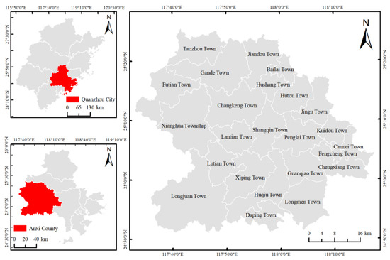
Figure 1.
Location map of the study area.
2.2. Data Source and Pre-Processing
The remote sensing image data of the study area were mainly obtained from Landsat/TM/TIRS/OLI published by Geospatial Data Cloud (http://www.gscloud.cn). As the scope of the remote sensing imagery does not encompass the entire study area, the image data were used for three time periods of 2010, 2015 and 2020, with a total of nine image data (Table 1). The image data of each time period were processed by image mosaic, cropping, radiation correction and atmospheric correction [29] and converted to a true color display by waveband combination and then compared with Google Earth Pro high-precision historical image data, and after visual interpretation and combined with field validation and calibration, according to the national standard of “Land Use Status Classification” (GB/721010-2017), combined with the research needs, the maximum likelihood method [30] was used to classify the study area into a total of nine land classes, including forest land; shrubs; grassland; arable land; tea gardens; orchards; construction land (residential, industrial and mining lands and towns); mudflats and water bodies. The overall accuracy of the classification of each of these periods was 87.63%, 86.92% and 88.32%, respectively, to meet the needs of the study. Among them, the data of tea-related population density and gross tea product in Anxi County were unified by GIS kriging interpolation, cropping, resampling and other operations with projection coordinates and a spatial resolution of 30 m. The data sources required for land use simulation are as follows (Table 1 and Table 2).

Table 1.
Remote sensing image information data.
Table 2.
Data required to simulate the projected study area for 2030 land use.
2.3. Methods
2.3.1. InVEST Habitat Quality Model
In this study, the InVEST model was applied to quantitatively assess habitat quality in the study area [31], which requires the input of land use data and combines the sensitivity of different land use types and the distance and mode of impact of threat sources of stress to map habitat quality [32]. Habitat quality depends on the proximity of habitats to threat sources and the ecological suitability of these habitats, and usually, habitat quality increases as the intensity of nearby land use decreases [33]. The equations are as follows:
where Dxj, R, Wr, yr and ry denote the habitat degradation index, the number of threat factors, the weight of threat factor r, the number of threat factor grids and the value of threat factor on the grids, respectively; irxy denotes the distance between the habitat and the threat source and the spatial impact of the threat; β is the factor to mitigate the impact of the threat on the habitat through various conservation policies (i.e., the degree of legal protection, with the area protected by law being 0 and the rest being 1); Sjr is the sensitivity of habitat type j to threat factor r; dxy is the linear distance between grids x and y; drmax is the maximum distance of the threat source r and drmax is the sensitivity of the threat source r to threat factor r. Sjr is the sensitivity of habitat type j to threat factor r, dxy is the linear distance between raster x and raster y and drmax is the maximum threat distance of threat source r. The higher the calculated score, the greater the threat of the threat factor to the habitat and the higher the degree of habitat degradation. The threat sources, maximum impact distance and weights of this study were obtained by referring to the relevant literature combined with the actual study area (Table 3) [31,34,35,36].
Table 3.
Threat sources and their maximum impact distances, weights and attenuation types.
Based on the above habitat degradation degree results, the habitat quality assessment equation is
where Qxj is the habitat quality index of raster x in land use j; Hj is the habitat suitability of habitat type j, ranging from 0 to 1; k is the half-saturation constant, usually 1/2 of the maximum value of habitat degradation and z is the normalization constant, usually set to 2.5. The data to be entered into this module include land use, major threat factors, threat source factor weights and impact distances, land use sensitivity to each threat source and sensitivity to each threat source, etc. This study refers to the InVEST model user’s guide manual and previous research results for the settings [37,38]. The sensitivity table for the different land use types is a required parameter setting in the Habitat Quality module of the InVEST model. It reflects the threat level of each threat source to each existing land type and the suitability of the existing land type and takes values in the range [0, 1]. The better the habitat of the species, the higher the degree of suitability. The coefficient of the threat source is the degree of impact of the threat source on each species (Table 4).
Table 4.
Sensitivity of different land use types to threat sources.
2.3.2. Space Autocorrelation
Spatial autocorrelation is an important indicator to test whether an element is correlated with its neighboring spatial elements [39]. A spatial autocorrelation analysis can be used to describe the distribution of spatial homogeneity of habitat quality within the study area [40,41,42]. In this study, global spatial autocorrelation (Global Moran’s I) and local spatial autocorrelation (Local Moran’s I) were used to measure the aggregation and divergence characteristics of spatial variation in habitat quality and to explore whether spatial variation has the phenomenon of high-value clustering and low-value clustering, through which the analysis can determine the habitat quality. The analysis can determine the locations where high or low value areas are clustered in a space.
Global Moran’s I is used to measure the interrelationship of spatial elements, and its value is between [−1, 1], and the larger the absolute value, the stronger the spatial autocorrelation. The calculation formula is:
where denotes the number of study objects, Xi is the observed value and is the mean value of . is the sum of all weights. is the spatial connection matrix between study objects i and j.
The results of the Moran indices were tested for significance with the following equation:
where and is the variance of I. ∣∣ > 1.96 indicates significant spatial autocorrelation. When −1.96 < < 1.96, it means the spatial autocorrelation is not significant.
Local Moran’s I is the decomposition of Moran’s I into individual regional units. That is, the LISA (Local Indicators of Spatial Association) clustering map has five types of local spatial aggregation, which are high–high (HH), low–low (LL), low–high (LH), high–low (HL) and insignificant. For a certain spatial unit i:
where , , and have the same meanings as Equations (5) and (6).
2.3.3. PLUS Model
The PLUS model is a new land use simulation model based on metacellular automata, which has advantages in studying the causes of land use change and dynamically simulating changes in multiple land uses, especially forest and grassland patches [43]. By extracting samples of the inter-transformation of various types of land use between two periods of land use data for training, the future land use is simulated based on the transformation probability, and the random forest algorithm is used to calculate the expansion of various types of land use and the driving factors to obtain the development probability of various types of land use and the contribution of the driving factors to the expansion of various types of land use during that time period, which is then combined with the generation of random patches and the setting of the transfer transition matrix to determine the PLUS model mainly consists of the following modules:
- (1)
- Land Expansion Analysis Strategy (LEAS) module
The LEAS is an analysis of land use data for two dates, and the growth patches of each changing land use type are used to obtain the change pattern of land use types, which can be used to characterize land use changes in a specific time interval, and the Random Forest Classification (RFC) algorithm is used to explore the relationship between the growth of different land use types and multiple drivers and to obtain the development probability of each land use type, calculated as [19]:
where is a vector consisting of the driving factors, is the number of decision trees; takes the value of 0 or 1—1 means other land use types can be transformed into land use type k, and 0 means other land types cannot be transformed into land type k, is the predicted land use type calculated at the decision tree of n, is the exponential function of the decision tree and is the probability of the growth of land use type k at spatial unit i.
- (2)
- CA model based on multi-class random patch seeding (CARS)
CARS is a scenario-driven land use simulation model based on metacellular automata that simulates the land use distribution pattern mainly by obtaining the development probabilities of various types of land uses. The total probability of conversion of land use type k, , is formulated as [19]:
where is the probability of growth of land use type on cell , is the domain effect of cell and is the effect of the future land use demand, calculated as [44]:
where is the total number of grid cells occupied by the th land use type in the last iteration in the th × th window; w is the weight between different land use types with a default value of 1 and D is the difference between the current demand and future demand of land use type at the st and nd iterations, respectively.
- (3)
- Related parameter setting
The LEAS parameters are set as follows: the value of the decision tree is set to 20, the sampling rate is 0.01 by default, mTry does not exceed the number of driving factors and is set to 9 and the number of parallel threads is set to 1.
The CARS parameters are set as follows: the neighborhood range is set to the default value of 3, Thread is set to 1, the decreasing threshold coefficient is 0.5, the diffusion coefficient is 0.1 and the random patch seed probability is 0.0001.
Three development scenarios are set: Different development strategies lead to changes in the structure of land use types, which, in turn, affect the quality of regional habitats [45]. Exploring land use types under different development scenarios in the study area is important to guide land planning and sustainable regional development [46]. To this end, in this study, three scenarios of natural development, arable land conservation and integrated development were used to simulate and predict land use in the study area under three development scenarios by changing the transfer rules of different land use types. In the natural development scenario (scenario 1), the development of each land use type continues the current development trend without adjustment; in the arable land protection scenario (scenario 2), arable land is protected and conversion of arable land to other land uses is restricted; in the integrated development scenario (scenario 3), the transfer rules of each land use type are proposed by considering food security, ecological protection, urbanization development and high-quality development of the tea industry in the study area [47,48,49]. The land use type transfer rules for different scenarios are shown in Table 5.
Table 5.
Different scenario transfer matrix settings.
- (4)
- Land use simulation prediction drivers
In this paper, drawing on the established research results on the drivers of land use change [50,51,52] and considering the actual situation of the study area, a total of nine drivers were finally selected from both socioeconomic and natural climatic aspects, including tea-related population density in the study area, total tea production value in the study area, average annual temperature, average annual precipitation, DEM, slope, distance from the highway, distance from the railroad and distance from the main road (Figure 2).
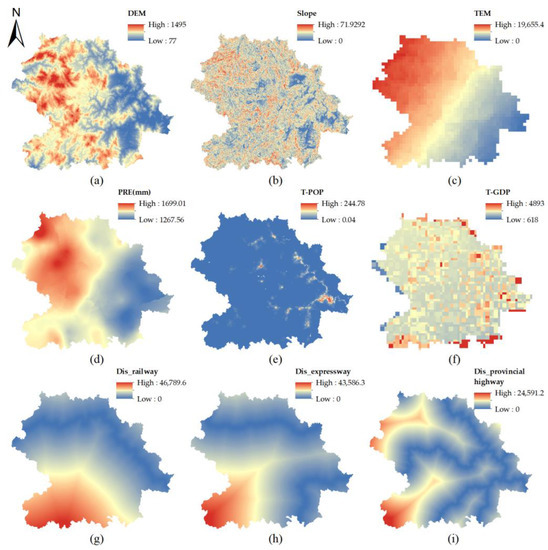
Figure 2.
Spatial distribution of land use drivers. (a) DEM; (b) slope; (c) average annual temperature; (d) average annual precipitation; (e) tea-related population density; (f) total tea production value; (g) distance to railroad; (h) distance to highway; (i) distance to provincial road.
- (5)
- Accuracy test
The land use map of 2010–2015 and the suitability raster atlas were input into the CARS module, and the land use structure in 2020 predicted by the Markov chain model was simulated to obtain the predicted land use map of the study area in 2020. The Kappa coefficient of the 2020 prediction map was 0.742, with an overall accuracy of 83.72%, which met the needs of the study. The Kappa coefficient for 2020 was 0.742, with an overall accuracy of 83.72%, which met the needs of the study. Then, based on this, we simulated the land use changes under different scenarios for 2030 with the relevant parameter settings.
3. Results
3.1. Spatial and Temporal Evolution of Land Use
3.1.1. Spatial Change Pattern of Land Use from 2010 to 2020
From 2010 to 2020, the main land use types in the study area are forest land, tea plantation, arable land and construction land. Among them, forest land is the dominant land use type, accounting for more than 50% of the total area of the study area; tea plantation has been the largest land use type in the study area for economic crops, now accounting for 25.59% of the total area, and the area of tea plantation has increased by 145.5606 km2 during the last 10 years. In the past 10 years, the area of each land use type has changed to different degrees, among which is the land use type with the largest change, arable land, which has decreased by 269.8209 km2 during the 10 years. The area decreased by 269.8209 km2, though the proportion of construction land area increased from 5.60% in 2010 to 8.26% in 2020, showing an increasing trend (Figure 3 and Table 6).
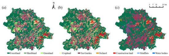
Figure 3.
Map of land use types in the study area for 2010–2020. (a) 2010; (b) 2015; (c) 2020.
Table 6.
Land use area and share of the study area by period, 2010–2020.
3.1.2. Land Use Simulation under Different Scenarios
From the results of different simulations (Figure 4 and Table 7), it can be seen that the areas of three major land categories, namely forest land, grassland and tea plantation, in Scenario 1 have further expanded, increasing by 120.5514 km2, 13.2246 km2 and 106.2405 km2, respectively, compared to 2020, with the largest increase in grassland area (200.82%). The areas of the remaining six land types show different magnitudes of decreases; among which, the areas of construction land and arable land decrease most significantly by 157.6107 km2 and 56.3940 km2, respectively, compared to 2020.
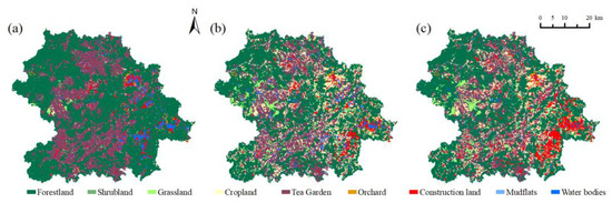
Figure 4.
Map of different scenarios of land use types in the study area in 2030. (a) Scenario 1; (b) scenario 2; (c) scenario 3.
Table 7.
Area and percentage changes of different scenario land use types in the study area.
The areas of forest land, grassland, arable land and water bodies in Scenario 2 further expand compared to 2020, increasing by 120.6099 km2, 11.133 km2, 272.9106 km2 and 0.945 km2, respectively, with the largest expansion being arable land (265.86%). The areas of the remaining five land types show different magnitudes of decrease, and the area of tea plantations decreases the most (246.465 km2).
The areas of the four major land categories of grassland, arable land, construction land and mudflats in Scenario 3 further expand compared to 2020, increasing by 106.7031 km2, 283.0302 km2, 10.0854 km2 and 0.2448 km2, respectively, with the largest increase in the area of arable land (283.0302 km2). The remaining five land types show different magnitudes of decrease in areas, with the largest decrease in forest land area (207.4815 km2), followed by tea plantations (165.5559 km2).
3.2. Spatial and Temporal Characteristics of Habitat Quality
Habitat quality refers to the ability of the ecological environment to provide suitable conditions for the survival of organisms and is one of the important indicators for the sustainable development and ecosystem service functions of the region, while land is the most basic carrier for biological habitats and the operation of various ecosystems. Therefore, it is important to explore the spatial and temporal evolution of habitat quality in the study area and the characteristics of changes in different scenarios to guide the formulation of land policies and achieve the high-quality development of the tea industry in the study area.
3.2.1. Spatial and Temporal Evolution of Habitat Quality from 2010 to 2020
The mean values of habitat quality in the study area in 2010, 2015 and 2020 were 0.6502, 0.6334 and 0.6919, respectively, and the overall habitat quality in the study area was at a high level, with an overall increase in the study area from 2010 to 2020, with an increment of 0.0417. The habitat quality results were classified into five classes: low (0–0.2), low (0.2–0.4), medium (0.4–0.6), high (0.6–0.8) and high (0.8–1). The results showed that the areas of habitat quality in the high, high and low classes showed trends of decreasing and then increasing, while the areas of habitat quality in the medium and low classes showed trends of increasing and then decreasing during the 10-year period. Overall, the study area was dominated by high habitat quality classes, with an area increase of 152.9766 km2, while the area of low habitat quality areas decreased by 192.7053 km2 (Table 8 and Figure 5). Habitat quality showed a more obvious spatial autocorrelation with Moran’s I values of 0.6347, 0.6374 and 0.6478 during 2010–2020, respectively. In terms of spatial distribution, the low–low agglomeration area gradually decreased in the northwestern and southern regions of the study area over time, which was mainly due to the expansion of tea plantations in the northwestern and southern regions (Table 9 and Figure 6).
Table 8.
Area and percentage of habitat quality in each class.
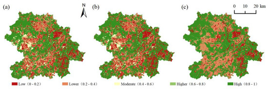
Figure 5.
Habitat quality in the study area from 2010 to 2020. (a) 2010; (b) 2015; (c) 2020.
Table 9.
The 2010–2020 habitat quality in the study area of Moran’s I.
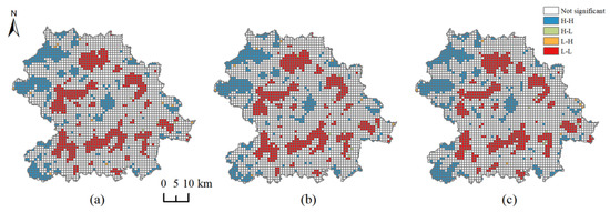
Figure 6.
The 2010–2020 LISA maps of habitat quality in the study area. (a) 2010; (b) 2015; (c) 2020.
To further explore the spatial and temporal dynamics of habitat quality in the study area, the habitat quality changes were calculated for each image element and classified as strongly degraded (−1 to −0.5), slightly degraded (−0.5 to −0.1), remained stable (−0.1–0.1), slight improvement (0.1–0.5) and strong improvement (0.5–1), for a total of five classes. The results of the study showed (Figure 7 and Table 10) that the habitat quality remained stable in most areas of the study area during the 10-year period, with an area of 2232.9036 km2, accounting for 74.70% of the total area of the study area, but the improved areas were always larger than the degraded areas, the strongly improved areas were concentrated in the western part of the study area and the strongly degraded areas were concentrated in the southern part of the study area. During 2010–2015, the overall habitat quality in the study area remained stable, accounting for 91.35% of the total area of the study area, while, during 2015–2020, the area and proportion of both improved and degraded areas in the study area increased, especially the proportions of the slightly improved and strongly improved areas in the study area, which increased by 6.64% and 9.07%, respectively.
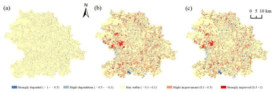
Figure 7.
Spatial and temporal variations in habitat quality in the study area from 2010 to 2020. (a) 2010; (b) 2015; (c) 2020.
Table 10.
Area and percentage of habitat quality changes in the study area from 2010 to 2020.
3.2.2. Habitat Quality Simulation Prediction Analysis under Different Scenarios
As shown in the prediction analysis (Table 11 and Figure 8), the mean habitat quality values of scenario 1 and scenario 2 were 0.7385 and 0.7162, respectively, compared with 0.6919 in 2020, and the mean habitat quality value of Scenario 3 was reduced to 0.6249, but their habitat quality was mainly of high grade, with an area share of more than 50%. Habitat quality under different scenarios showed more obvious spatial autocorrelation (Table 12 and Figure 9), with Moran’s I values of 0.6981, 0.6443 and 0.6676, respectively; in terms of spatial distribution, compared with 2020, the high–high agglomeration area of scenario 1 decreased in the northwest and southwest of the study area, which was mainly due to the expansion of tea plantations, and the low–low agglomeration area decreased in the east, which was mainly due to the high–high agglomeration area of scenario 2 decreasing in the southwest and central parts of the study area, which was mainly due to the expansion of tea plantations; the low–low agglomeration area of scenario 3 increased in the southeast, which was mainly due to the increase of construction land.
Table 11.
Area and proportion of each class of habitat quality for different scenarios in the study area in 2030.
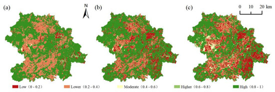
Figure 8.
Habitat quality in different scenarios in the study area in 2030. (a). Scenario 1; (b) scenario 2; (c) scenario 3.
Table 12.
Habitat quality under different scenarios in the study area in 2030 with Moran’s I.
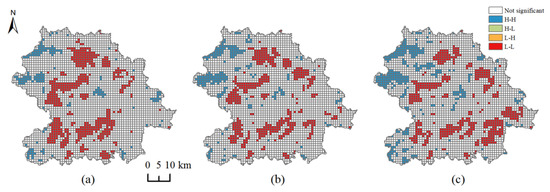
Figure 9.
LISA maps of habitat quality for different scenarios in the study area in 2030. (a) Scenario 1; (b) scenario 2; (c) scenario 3.
To further clarify the spatial variation characteristics of habitat quality under different scenarios in the study area in 2030, the ArcGIS raster calculator was used to calculate the difference between the habitat quality of different development scenarios and the habitat quality in 2020. The results show (Figure 10 and Table 13) that the habitat quality in the study area remains stable in most areas under each scenario in 2030, and they all account for more than 70% of the total area of the study area. The improved area is higher than that of the degraded area in scenario 1, and the improved area is mainly concentrated in the eastern region, mostly because the construction land in the eastern region is converted into woodland; the improved area and the degraded area in scenario 2 is about the same, the improved area is more concentrated in the southern region, mainly because the tea plantation is converted into woodland, the degraded area is mainly concentrated in the western region and the woodland and water bodies are converted into grassland and cropland; the degraded area in scenario 3 is larger than that of the improved area. The degraded area is larger than that of the improved area, and the degraded area is mainly concentrated in the west and southeast of the study area, which is mostly due to the conversion of forest land to grassland and construction land in the west and southeast, respectively. The improvement area is mainly concentrated in the south, and the main reason is that the tea plantation is transformed into forest land.
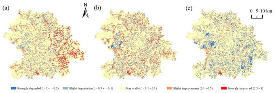
Figure 10.
Spatial and temporal variations in habitat quality for different scenarios in the study area in 2030. (a) Scenario 1; (b) scenario 2; (c) scenario 3.
Table 13.
Area and percentage of habitat quality changes in the study area in 2030 for different scenarios.
4. Discussion
The PLUS model and InVEST model are used to predict the land use distribution pattern of the study area in 2030 under different scenarios based on the current land use situation; analyze the spatial and temporal evolution characteristics of habitat quality in the study area and explore the characteristics of habitat quality changes under different land use scenarios, which are important for improving the ecological environment of the study area, guiding the formulation of land policies and realizing the high-quality development of the tea industry in the study area.
- (1)
- Impact of land use change on habitat quality
During 2010–2015, the habitat quality of the study area showed a decreasing trend, and in response to the accelerated pace of new rural construction during this period, the area of construction land grew more rapidly during this period, with the expansion of the threat source area, which, in turn, reduced the habitat quality of the study area. During 2015–2020, the habitat quality of the study area showed an increasing trend due to the fact that the study area came from the tea pesticide residue incident during this period, the tea recovery of the consumer market, the influence of the tea industry policy and the influx of a large number of tea production operators, resulting in the reclamation of a large amount of arable land into tea gardens, and although tea gardens were also one of the sources of habitat quality threats, the degree of threat impact was lower compared to arable land, and the expansion of the construction land area in this period was weakened, which, in turn, improved the habitat quality in the study area. Compared to 2020, the habitat quality of scenario 1 was improved, and the construction habitat quality in scenario 1 improved compared to 2020 because the area of land under construction was significantly reduced, which led to the improvement in habitat quality; scenario 2 improved the habitat quality mainly because the area of land under construction was significantly reduced and scenario 3 decreased the habitat quality mainly because the area of forest land was reduced and the area of cropland increased.
- (2)
- Strengths of the model used in this study
The InVEST model used in this study is widely used due to the use of fewer parameters and stronger visualization, and the model is relatively mature and has some advantages over other traditional methods in spatial representation and dynamic studies. In this study, the PLUS model integrates a new land use expansion analysis strategy, which can better explore the contribution of the causal factors and drivers of various types of land use changes to the expansion of various types of land uses in that time period and can better simulate the changes at the patch level of multiple types of land uses. Compared with other models, such as FLUS, the PLUS model has a higher accuracy in land use simulation, which can overcome the problem of accuracy of simulation data in large-scale research areas. The combined application of the two models better reveals the evolution of the land use structure and habitat quality under current land development conditions in the study area.
- (3)
- Limitations of the study
In this study, the dynamics of habitat quality in the study area from 2010 to 2020 were explored first, followed by the prediction of land use distribution patterns under three scenarios in the study area in 2030 using the PLUS model, and the spatial and temporal characteristics of habitat quality under different development scenarios were assessed using the InVEST model. However, this study has some limitations. First, in the InVEST model habitat quality assessment, the model still has some shortcomings. On the one hand, the simple accumulation of the effects of each threat factor of the model is not equal to the combined effect of each threat factor on habitat quality, and in some cases, the collective effect of multiple threat factors may be much larger than the sum of individual threat factors, which is not considered in the InVEST model, and further improvement of the model is needed. Secondly, in the selection of driving factors for the land use simulation, some of the data were difficult to obtain, so the driving factors were not considered comprehensively, but only natural, economic and traffic location factors were involved, and the future planning of the study area was not considered enough, such as permanent basic agricultural land and ecological protection red lines, which should be further improved in the follow-up study to make the simulation results more scientific.
- (4)
- Strategies for optimizing land use in tea plantations
Our study shows that the expansion of tea plantations has a negative impact on the quality of regional habitats. Therefore, in order to balance the economic development of tea in Anxi County with the regional habitat quality and biodiversity supply, we suggest implementing the policy of “returning tea to forest” and “returning tea to farming” in some areas of tea plantations. For example, the policy of “returning tea to forest” should be implemented in the northwestern part of the study area, mainly because the slope of the area is high, the area of tea plantations is small and scattered and the excessive cultivation of tea plantations leads to the reduction of biodiversity. In contrast, the habitat quality in the southcentral region is generally lower and the slope gentler compared with the suitability of cultivated land compared to tea plantations. Therefore, the implementation of the “return of tea to cultivation” policy in this area is conducive to ensuring food production in the study area. This is also in line with the food security policy of Anxi County.
5. Conclusions
This study analyzed the spatial and temporal evolutions of land use in the study area from 2010 to 2020, used the PLUS model to simulate and predict land use changes in the study area for different development scenarios in 2030 and used the InVEST model to assess and predict the spatial and temporal evolution patterns of habitat quality in the study area, with the following conclusions:
- (1)
- From 2010 to 2020, the areas of forest land, tea plantations and water bodies in the study area decreased and then increased, the areas of irrigated grassland and arable land increased and then decreased, the areas of shrubs and construction land continued to increase and the area of orchards continued to decrease. Among them, forest land area increased the most, mainly in the northwestern part of the study area, followed by tea plantations, mainly in the northern and southern regions of the study area; arable land area decreased the most, with a large reduction in the study area, followed by grassland, mainly in the western and southwestern regions of the study area.
- (2)
- The prediction results of the PLUS model show that the land use distribution patterns under different scenarios in 2030 will change significantly. Compared with 2020, the areas of woodland, grassland and tea plantations in scenario 1 continue to increase, while the rest of the land use continues to decrease; the areas of woodland, grassland, cropland and water bodies in scenario 2 continue to increase, while the rest of the land use continues to decrease; the areas of grassland, cropland, construction land and mudflats in scenario 3 continue to increase, while the rest of the land use continues to decrease.
- (3)
- Habitat quality in the study area from 2010 to 2020 was generally at a high level with an upward trend. Ten years later, the study area was dominated by high-grade habitat quality, and the areas of low habitat quality were decreasing, but the areas of lower habitat quality were increasing. Habitat quality showed a more obvious spatial autocorrelation, and with the expansion of the tea plantation area, the low–low concentration area gradually decreased in the northwestern and southern regions of the study area. The changes in the spatial characteristics of habitat quality showed that the area maintaining a stable grade was the largest, the improved area was always larger than that of the degraded area, the strongly improved area was concentrated in the western part of the study area and the strongly degraded area was concentrated in the southern part of the study area.
- (4)
- Habitat quality in 2030 changed under different scenarios, except for scenario 3; the mean values of habitat quality in scenario 1 and scenario 2 were higher than that in 2020, while the proportion of high-grade area of habitat quality was greater than 50%. Habitat quality under different scenarios showed a more obvious spatial autocorrelation compared to 2020. Scenario 1 showed a decrease in high–high concentration areas in the northwestern and southwestern parts of the study area with the expansion of tea plantations and low–low concentration areas in the eastern part of the study area with the reduction in construction land area; scenario 2 showed a decrease in high–high concentration areas in the southwestern and central parts of the study area, with the expansion of tea plantations; scenario 3 showed a decrease in low–low concentration. The habitat quality of the study area remained stable in most areas of the study area in 2030 under all scenarios, accounting for more than 70% of the total study area. The improved area was higher than that of the degraded area in scenario 1, which was mainly due to the conversion of construction land to forest land in the eastern region; the improved area and degraded area in scenario 2 were approximately the same, with the improved area concentrated in the southern region and the degraded area concentrated in the western region; the degraded area was larger than that of the improved area in scenario 3, which was mainly due to the conversion of forest land to grassland and construction land in the western and southeastern regions, respectively.
Author Contributions
Conceptualization, W.L. (Wen Li); methodology, W.L. (Wen Li), S.F. and J.G.; software, J.G. and J.B.; validation, W.L. (Wen Li), W.L. (Wenxiong Lin) and S.F.; formal analysis, W.L. (Wen Li) and S.F.; investigation, J.G. and J.B.; resources, J.G.; data curation, W.L. (Wen Li) and W.L. (Wenxiong Lin); writing—original draft preparation, W.L. (Wen Li); writing—review and editing, S.F.; visualization, W.L. (Wen Li), J.G. and J.B.; supervision, S.F. and Z.W.; project administration, S.F. and funding acquisition, S.F. All authors have read and agreed to the published version of the manuscript.
Funding
This work was supported by the Fujian Agriculture and Forestry University Tea Industry Chain Science and Technology Innovation Team Project: Tea Industry Economy and Creativity Research (K1520012A08), Science and Education Special Project of Fujian Province: Science and Technology Integration and Mechanism of “Small Industrial Courtyard” for Special Modern Agriculture (K8120K01a), Fujian Agriculture and Forestry University’s “industry-creation integration” talent training practice platform construction based on industrial revitalization of tea economy (111420049) and Leisure agriculture and industry integration service team (11899170121).
Data Availability Statement
The data that support the findings of this study are available from the authors upon reasonable request.
Conflicts of Interest
The authors declare no conflict of interest.
References
- Liu, Y. Introduction to land use and rural sustainability in China. Land Use Pol. 2018, 74, 1–4. [Google Scholar] [CrossRef]
- Su, S.; Wan, C.; Li, J.; Jin, X.; Pi, J.; Zhang, Q.; Weng, M. Economic benefit and ecological cost of enlarging tea cultivation in subtropical China: Characterizing the trade-off for policy implications. Land Use Pol. 2017, 66, 183–195. [Google Scholar] [CrossRef]
- Haines-Young, R. Land use and biodiversity relationships. Land Use Pol. 2009, 26, S178–S186. [Google Scholar] [CrossRef]
- Zeng, B.; Zhang, F.; Zeng, W.; Yan, K.; Cui, C. Spatiotemporal heterogeneity in runoff dynamics and its drivers in a water conservation area of the upper yellow river basin over the past 35 years. Remote Sens. 2022, 14, 3628. [Google Scholar] [CrossRef]
- Vanwalleghem, T.; Gómez, J.A.; Amate, J.I.; De Molina, M.G.; Vanderlinden, K.; Guzmán, G.; Laguna, A.; Giráldez, J.V. Impact of historical land use and soil management change on soil erosion and agricultural sustainability during the Anthropocene. Anthropocene 2017, 17, 13–29. [Google Scholar] [CrossRef]
- Wu, J.; Luo, J.; Zhang, H.; Qin, S.; Yu, M. Projections of land use change and habitat quality assessment by coupling climate change and development patterns. Sci. Total Environ. 2022, 847, 157491. [Google Scholar] [CrossRef]
- He, J.; Huang, J.; Li, C. The evaluation for the impact of land use change on habitat quality: A joint contribution of cellular automata scenario simulation and habitat quality assessment model. Ecol. Model. 2017, 366, 58–67. [Google Scholar] [CrossRef]
- Tang, F.; Wang, L.; Guo, Y.; Fu, M.; Huang, N.; Duan, W.; Luo, M.; Zhang, J.; Li, W.; Song, W. Spatio-temporal variation and coupling coordination relationship between urbanisation and habitat quality in the Grand Canal, China. Land Use Pol. 2022, 117, 106119. [Google Scholar] [CrossRef]
- Wu, J.; Li, X.; Luo, Y.; Zhang, D. Spatiotemporal effects of urban sprawl on habitat quality in the Pearl River Delta from 1990 to 2018. Sci Rep. 2021, 11, 1–15. [Google Scholar] [CrossRef]
- Wang, B.; Cheng, W. Effects of land use/cover on regional habitat quality under different geomorphic types based on InVEST model. Remote Sens. 2022, 14, 1279. [Google Scholar] [CrossRef]
- Store, R.; Kangas, J. Integrating spatial multi-criteria evaluation and expert knowledge for GIS-based habitat suitability modelling. Landsc. Urban Plan. 2001, 55, 79–93. [Google Scholar] [CrossRef]
- Mammola, S.; Milano, F.; Vignal, M.; Andrieu, J.; Isaia, M. Associations between habitat quality, body size and reproductive fitness in the alpine endemic spider Vesubia jugorum. Glob. Ecol. Biogeogr. 2019, 28, 1325–1335. [Google Scholar] [CrossRef]
- Li, M.; Zhou, Y.; Xiao, P.; Tian, Y.; Huang, H.; Xiao, L. Evolution of Habitat Quality and Its Topographic Gradient Effect in Northwest Hubei Province from 2000 to 2020 Based on the InVEST Model. Land. 2021, 10, 857. [Google Scholar] [CrossRef]
- Sun, H.Y.; Gong, Q.Q.; Liu, Q.G.; Sun, P.L. Spatio-temporal evolution of habitat quality based on the land-use changes in Shandong Province. Chin. J. Soil Sci. 2022, 12, 15422. [Google Scholar]
- Dong, J.; Zhang, Z.; Liu, B.; Zhang, X.; Zhang, W.; Chen, L. Spatiotemporal variations and driving factors of habitat quality in the loess hilly area of the Yellow River Basin: A case study of Lanzhou City, China. J. Arid Land 2022, 14, 637–652. [Google Scholar] [CrossRef]
- Cong, W.; Sun, X.; Guo, H.; Shan, R. Comparison of the SWAT and InVEST models to determine hydrological ecosystem service spatial patterns, priorities and trade-offs in a complex basin. Ecol. Indic. 2020, 112, 106089. [Google Scholar] [CrossRef]
- Guan, D.; Li, H.; Inohae, T.; Su, W.; Nagaie, T.; Hokao, K. Modeling urban land use change by the integration of cellular automaton and Markov model. Ecol. Model. 2011, 222, 3761–3772. [Google Scholar] [CrossRef]
- Liu, X.; Liang, X.; Li, X.; Xu, X.; Ou, J.; Chen, Y.; Li, S.; Wang, S.; Pei, F. A future land use simulation model (FLUS) for simulating multiple land use scenarios by coupling human and natural effects. Landsc. Urban Plan. 2017, 168, 94–116. [Google Scholar] [CrossRef]
- Zhang, P.; Liu, L.; Yang, L.; Zhao, J.; Li, Y.; Qi, Y.; Ma, X.; Cao, L. Exploring the response of ecosystem service value to land use changes under multiple scenarios coupling a mixed-cell cellular automata model and system dynamics model in Xi’an, China. Ecol. Indic. 2023, 147, 110009. [Google Scholar] [CrossRef]
- Liang, X.; Guan, Q.; Clarke, K.C.; Liu, S.; Wang, B.; Yao, Y. Understanding the drivers of sustainable land expansion using a patch-generating land use simulation (PLUS) model: A case study in Wuhan, China. Comput. Environ. Urban Syst. 2021, 85, 101569. [Google Scholar] [CrossRef]
- Li, X.; Fu, J.; Jiang, D.; Lin, G.; Cao, C. Land use optimization in Ningbo City with a coupled GA and PLUS model. J. Clean Prod. 2022, 375, 134004. [Google Scholar] [CrossRef]
- Xu, L.; Liu, X.; Tong, D.; Liu, Z.; Yin, L.; Zheng, W. Forecasting urban land use change based on cellular automata and the PLUS model. Land 2022, 11, 652. [Google Scholar] [CrossRef]
- Meng, F.; Zhou, Z.; Zhang, P. Multi-Objective Optimization of Land Use in the Beijing–Tianjin–Hebei Region of China Based on the GMOP-PLUS Coupling Model. Sustainability 2023, 15, 3977. [Google Scholar] [CrossRef]
- Liu, S.; Liao, Q.; Xiao, M.; Zhao, D.; Huang, C. Spatial and temporal variations of habitat quality and its response of landscape dynamic in the three gorges reservoir area, China. Int. J. Environ. Res. Public Health 2022, 19, 3594. [Google Scholar] [CrossRef]
- Bai, L.; Xiu, C.; Feng, X.; Liu, D. Influence of urbanization on regional habitat quality: A case study of Changchun City. Habitat Int. 2019, 93, 102042. [Google Scholar] [CrossRef]
- Li, Y.; Duo, L.; Zhang, M.; Yang, J.; Guo, X. Habitat quality assessment of mining cities based on InVEST model—A case study of Yanshan County, Jiangxi Province. Int. J. Coal Sci. Technol. 2022, 9, 28. [Google Scholar] [CrossRef]
- Wei, L.; Zhou, L.; Sun, D.; Yuan, B.; Hu, F. Evaluating the impact of urban expansion on the habitat quality and constructing ecological security patterns: A case study of Jiziwan in the Yellow River Basin, China. Ecol. Indic. 2022, 145, 109544. [Google Scholar] [CrossRef]
- Xiao, L.; Cui, L.; Jiang, Q.O.; Wang, M.; Xu, L.; Yan, H. Spatial structure of a potential ecological network in Nanping, China, based on ecosystem service functions. Land 2020, 9, 376. [Google Scholar] [CrossRef]
- Ellis, E.A.; Porter-Bolland, L. Is community-based forest management more effective than protected areas?: A comparison of land use/land cover change in two neighboring study areas of the Central Yucatan Peninsula, Mexico. For. Ecol. Manag. 2008, 256, 1971–1983. [Google Scholar] [CrossRef]
- Sun, J.; Yang, J.; Zhang, C.; Yun, W.; Qu, J. Automatic remotely sensed image classification in a grid environment based on the maximum likelihood method. Math. Comput. Model. 2013, 58, 573–581. [Google Scholar] [CrossRef]
- Sallustio, L.; De Toni, A.; Strollo, A.; Di Febbraro, M.; Gissi, E.; Casella, L.; Geneletti, D.; Munafò, M.; Vizzarri, M.; Marchetti, M. Assessing habitat quality in relation to the spatial distribution of protected areas in Italy. J. Environ. Manag. 2017, 201, 129–137. [Google Scholar] [CrossRef] [PubMed]
- Zhu, J.; Ding, N.; Li, D.; Sun, W.; Xie, Y.; Wang, X. Spatiotemporal analysis of the nonlinear negative relationship between urbanization and habitat quality in metropolitan areas. Sustainability 2020, 12, 669. [Google Scholar] [CrossRef]
- Cheng, F.; Liu, S.; Hou, X.; Wu, X.; Dong, S.; Coxixo, A. The effects of urbanization on ecosystem services for biodiversity conservation in southernmost Yunnan Province, Southwest China. J. Geogr. Sci. 2019, 29, 1159–1178. [Google Scholar] [CrossRef]
- Sharp, R.; Tallis, H.T.; Ricketts, T.; Guerry, A.D.; Wood, S.A.; Chaplin-Kramer, R.; Nelson, E.; Ennaanay, D.; Wolny, S.; Olwero, N. InVEST 3.2. 0 User’s Guide; The Natural Capital Project; Stanford University: Standford, CA, USA, 2018. [Google Scholar]
- Mashizi, A.K.; Escobedo, F.J. Socio-ecological assessment of threats to semi-arid rangeland habitat in Iran using spatial models and actor group opinions. J. Arid. Environ. 2020, 177, 104136. [Google Scholar] [CrossRef]
- Terrado, M.; Sabater, S.; Chaplin-Kramer, B.; Mandle, L.; Ziv, G.; Acuña, V. Model development for the assessment of terrestrial and aquatic habitat quality in conservation planning. Sci. Total Environ. 2016, 540, 63–70. [Google Scholar] [CrossRef]
- Du, S.X.; Rong, Y.J. The biodiversity assessment of land use in Shanxi Province based on InVEST model. Environ. Sustain. Dev. 2015, 40, 65–70. [Google Scholar]
- Liu, F.; Xu, E. Comparison of spatial-temporal evolution of habitat quality between Xinjiang Corps and Non-corps Region based on land use. J. Appl. Ecol. 2020, 31, 2341–2351. [Google Scholar]
- Getis, A. A history of the concept of spatial autocorrelation: A geographer’s perspective. Geogr. Anal. 2008, 40, 297–309. [Google Scholar] [CrossRef]
- Zhu, C.; Zhang, X.; Zhou, M.; He, S.; Gan, M.; Yang, L.; Wang, K. Impacts of urbanization and landscape pattern on habitat quality using OLS and GWR models in Hangzhou, China. Ecol. Indic. 2020, 117, 106654. [Google Scholar] [CrossRef]
- Moore, B.D.; Lawler, I.R.; Wallis, I.R.; Beale, C.M.; Foley, W.J. Palatability mapping: A koala’s eye view of spatial variation in habitat quality. Ecology 2010, 91, 3165–3176. [Google Scholar] [CrossRef]
- Chen, L.; Wei, Q.; Fu, Q.; Feng, D. Spatiotemporal evolution analysis of habitat quality under high-speed urbanization: A case study of urban core area of China Lin-Gang Free Trade Zone (2002–2019). Land 2021, 10, 167. [Google Scholar] [CrossRef]
- Li, C.; Wu, Y.; Gao, B.; Zheng, K.; Wu, Y.; Li, C. Multi-scenario simulation of ecosystem service value for optimization of land use in the Sichuan-Yunnan ecological barrier, China. Ecol. Indic. 2021, 132, 108328. [Google Scholar] [CrossRef]
- Gu, C.; Hu, L.; Zhang, X.; Wang, X.; Guo, J. Climate change and urbanization in the Yangtze River Delta. Habitat Int. 2011, 35, 544–552. [Google Scholar] [CrossRef]
- Quintas-Soriano, C.; Castro, A.J.; Castro, H.; García-Llorente, M. Impacts of land use change on ecosystem services and implications for human well-being in Spanish drylands. Land Use Pol. 2016, 54, 534–548. [Google Scholar] [CrossRef]
- Lou, Y.; Yang, D.; Zhang, P.; Zhang, Y.; Song, M.; Huang, Y.; Jing, W. Multi-scenario simulation of land use changes with ecosystem service value in the Yellow River Basin. Land 2022, 11, 992. [Google Scholar] [CrossRef]
- Wang, H.; Zhang, C.; Yao, X.; Yun, W.; Ma, J.; Gao, L.; Li, P. Scenario simulation of the tradeoff between ecological land and farmland in black soil region of Northeast China. Land Use Pol. 2022, 114, 105991. [Google Scholar] [CrossRef]
- Pan, Z.; He, J.; Liu, D.; Wang, J. Predicting the joint effects of future climate and land use change on ecosystem health in the Middle Reaches of the Yangtze River Economic Belt, China. Appl. Geogr. 2020, 124, 102293. [Google Scholar] [CrossRef]
- Liu, J.; Jin, X.; Xu, W.; Gu, Z.; Yang, X.; Ren, J.; Fan, Y.; Zhou, Y. A new framework of land use efficiency for the coordination among food, economy and ecology in regional development. Sci. Total Environ. 2020, 710, 135670. [Google Scholar] [CrossRef]
- Liu, J.; Zhang, Z.; Xu, X.; Kuang, W.; Zhou, W.; Zhang, S.; Li, R.; Yan, C.; Yu, D.; Wu, S. Spatial patterns and driving forces of land use change in China during the early 21st century. J. Geogr. Sci. 2010, 20, 483–494. [Google Scholar] [CrossRef]
- Wu, H.; Lin, A.; Xing, X.; Song, D.; Li, Y. Identifying core driving factors of urban land use change from global land cover products and POI data using the random forest method. Int. J. Appl. Earth Obs. Geoinf. 2021, 103, 102475. [Google Scholar] [CrossRef]
- Zhao, B.; Li, S.; Liu, Z. Multi-Scenario Simulation and Prediction of Regional Habitat Quality Based on a System Dynamic and Patch-Generating Land-Use Simulation Coupling Model—A Case Study of Jilin Province. Sustainability 2022, 14, 5303. [Google Scholar] [CrossRef]
Disclaimer/Publisher’s Note: The statements, opinions and data contained in all publications are solely those of the individual author(s) and contributor(s) and not of MDPI and/or the editor(s). MDPI and/or the editor(s) disclaim responsibility for any injury to people or property resulting from any ideas, methods, instructions or products referred to in the content. |
© 2023 by the authors. Licensee MDPI, Basel, Switzerland. This article is an open access article distributed under the terms and conditions of the Creative Commons Attribution (CC BY) license (https://creativecommons.org/licenses/by/4.0/).