Article

Quantifying the Effects of Green-Town Development on Land Surface Temperatures (LST) (A Case Study at Karizland (Karizboom), Yazd, Iran)

by
Mohammad Mansourmoghaddam
1,
Negar Naghipur
2,
Iman Rousta
3,4,*,
Seyed Kazem Alavipanah
5,
Haraldur Olafsson
6 and
Ashehad A. Ali
7,*
1
Center for Remote Sensing and GIS Studies, Shahid Beheshti University, Tehran 1983969411, Iran
2
Department of Remote Sensing, Yazd University, Yazd 8915818411, Iran
3
Department of Geography, Yazd University, Yazd 8915818411, Iran
4
Institute for Atmospheric Sciences-Weather and Climate, University of Iceland and Icelandic Meteorological Office (IMO), Bustadavegur 7, IS-108 Reykjavik, Iceland
5
Department of Remote Sensing and GIS, The University of Tehran, Tehran 1417935840, Iran
6
Institute for Atmospheric Sciences-Weather and Climate, Department of Physics, University of Iceland and Icelandic Meteorological Office (IMO), Bustadavegur 7, IS-108 Reykjavik, Iceland
7
Department of Bioclimatology, University of Göttingen, 37077 Göttingen, Germany
*
Authors to whom correspondence should be addressed.
Land 2023, 12(4), 885; https://doi.org/10.3390/land12040885
Submission received: 8 March 2023 / Revised: 30 March 2023 / Accepted: 10 April 2023 / Published: 14 April 2023

Abstract

:
Several earth science investigations depend heavily on knowing the surface energy budget and determining surface temperature. The primary factor affecting the energy balance in the surface physical processes of the planet is the land surface temperature (LST). Even in the case of small-scale green areas like local parks, plants have a significant impact on the climate of cities. The goal of this study was to estimate the construction-related impacts of the Karizland green town (green belt) on the LST of its surroundings over time, for the years 2013 (before construction began), 2015, 2020 and 2022 (after construction was completed). LST values and hot spot analyses were employed for thermal condition evaluation purposes on Landsat-8 satellite images, and normalized difference vegetation index (NDVI) and fractional vegetation cover (FVC) indices were used for examining the vegetation change. The results showed that after the establishment of the green town, the mean NDVI and FVC grew by 275% and 950%, respectively, compared to the initial period, which resulted in the addition of approximately 208.35 ha of green space to the study area. In this regard, the results showed that after these changes, compared to the first period, the mean LST decreased by 8%. In addition, the area of the class of hotspot analysis with less than 90% confidence increased by 9%. The results illustrated that almost 20% of the data in the LST range was below 55 °C in 2013, near 57 °C in 2015, and around 51 °C in 2020 and 2022. The results also showed a negative relationship between the distance from the established settlement and the values of NDVI and FVC in 2022 of 91% and 89% and in 2020 of 67% and 69%, respectively. Every year, LST has had a significant negative relationship with the NDVI and FVC of that year and a positive relationship with the LST of the following years, such that the correlation decreases in later years. In order to control LST and the temperature surrounding cities, this research strongly advises managers to develop these green towns.

1. Introduction

Climate change and rapidly increasing global urbanization are the two concerns that urban planners face in the twenty-first century [1]. The planet’s surface is one of the key elements in earth sciences. The planet’s surface net energy, which is controlled by energy input, surface discharge, humidity, and atmospheric air movement, determines this physical property. Understanding the surface energy budget and calculating surface temperature are crucial in many earth science studies, including those involving urban expansion [2,3], management of water resources, natural disasters, and the climate. Land surface temperature (LST) is the main determinant of the energy balance in the earth’s surface physical processes [4]. The study of LST, along with other factors such as evapotranspiration and soil salinity, are also useful in cases such as the effects of global warming on food security [5] and energy consumption [6].
The urban environment’s temperature is affected by a wide range of climatic, geographic, and human factors, and it mostly reflects local climate characteristics, which are different from atmospheric temperature. The urban environment’s temperature changes both indoors and outside since there are different land uses. Because of this, recent research has centered more on identifying these changes in the urban environment [7,8]. Urban green spaces are essential for maintaining the urban environment, controlling urban temperature, and balancing climate change in addition to improving urban landscapes [9], environmental soil properties [10], and spatial susceptibility patterns [11]. Plants cool the air around them through shade, evaporation, and other methods to enhance the urban environment [12].
One of the factors affecting the microclimate in urban areas investigated is the utilization of plants [13]. The influence of plants on the climate of city environments is enormous, even in the case of small-scale green spaces like neighborhood parks [14,15]. The existence of trees, grass, and other plant life causes green spaces to have cooler temperatures than other neighboring metropolitan areas [16]. It is thought that this phenomenon prevents the temperature of the air around from increasing. Often, the temperature in green areas is lower than that of adjacent locations [17]. Cooler air is transported from green parts to nearby areas. The amount of cooling experienced by the nearby areas changes with an increase in the size of the green space and the percentage of that space that is covered by trees [1].
Remote sensing techniques can provide a fast and efficient means of mapping landforms, which can be a crucial first step in managing the Earth’s surface [18]. Quantifiable LST data may be gathered using remote sensing thermal sensors and used to monitor land cover changes. Remote sensing is essential for estimating physical properties important to thermal research. A number of multispectral and thermal sensors can be used for urban vegetation indices and LST [19] studies. The two most used remote sensing vegetation indices are the normalized vegetation index (NDVI) and fractional vegetation index (FVI). There are two methods utilized to retrieve correct FVC values: field measurement and remote sensing retrieval. The traditional method for obtaining FVC is field measurement, which combines sampling, visual estimation, and the use of optical measuring tools (e.g., photography). Three techniques may be used to get FVC from remote sensing: the empirical model, the physical model, and machine learning techniques. FVC is estimated using an empirical model using either a straightforward statistical model or a regression relationship. The FVC is often computed from the NDVI once an empirical link between the two has been established [20].
Previous studies such as Zare et al. (2021) highlight the potential of remote sensing data and satellite image analysis in observing changes in earth and natural resources [21]. Amani-Beni et al. (2019) investigated the connection between urban greening trends and the cooling impact in the Olympic Forest’s environs, a park in Beijing. The impervious LST of forestland and waterbodies might be cooled by 6.51% and 12.82%, respectively, according to the results. LST decreased by 0.4 °C for every 10% increase in green space, while it rose by 0.15 °C for every kilometer of distance from the forest park. The green space patterns’ aggregation index (AI) and biggest patch index (LPI) showed a substantial negative connection with surface temperature [22]. Another study by Sun et al. (2017) investigated the utilization of urban green space in a long belt-shaped park (around 9 km) in Beijing to raise the surrounding city’s average temperature. The findings indicated that the temperature drops to roughly 2 degrees Celsius up to 90 m from the researched green area’s edge [23]. Research conducted by Zhao et al. (2022) related to the construction of Kunlun Mountain national park in China, built in order to reduce the effects of climate change, has shown an increase in the capacity of the carbon sink, and has predicted that this will improve similarly with the implementation of park management and control measures [24,25]. In a study by Di Leo et al. (2016), the impact of urbanization and green infrastructure on the temperature of the urban surface in Bobo-Dioulasso, Burkina Faso, sub-Saharan Africa, was examined. Urbanization and LSTs were geographically and temporally explored using the geospatial data and methods that are now available. The study also examined how certain urban green infrastructure locations affected LSTs. The findings revealed rising temperatures and rates of urbanization throughout time and location. However, the LST in regions with green infrastructure was in fact lower than that in nearby impermeable, urbanized areas [26,27].
Since vegetation has a cooling effect on LST [28,29] and also the study of the earth’s surface temperature is important due to its effect on global warming and human well-being, the present research aims to quantify the effect of creating a green town called Karizland (Karizboom) which includes tree and shrub cover (Figure 1) near the city of Yazd (which is located in the hot and dry central region of Iran and faces a lack of green space per capita [30]). The importance of this study is in highlighting the effect of creating such settlements and encouraging the authorities to establish such settlements in other places in order to manage per capita vegetation and LST.

2. Materials and Methods

2.1. Study Area

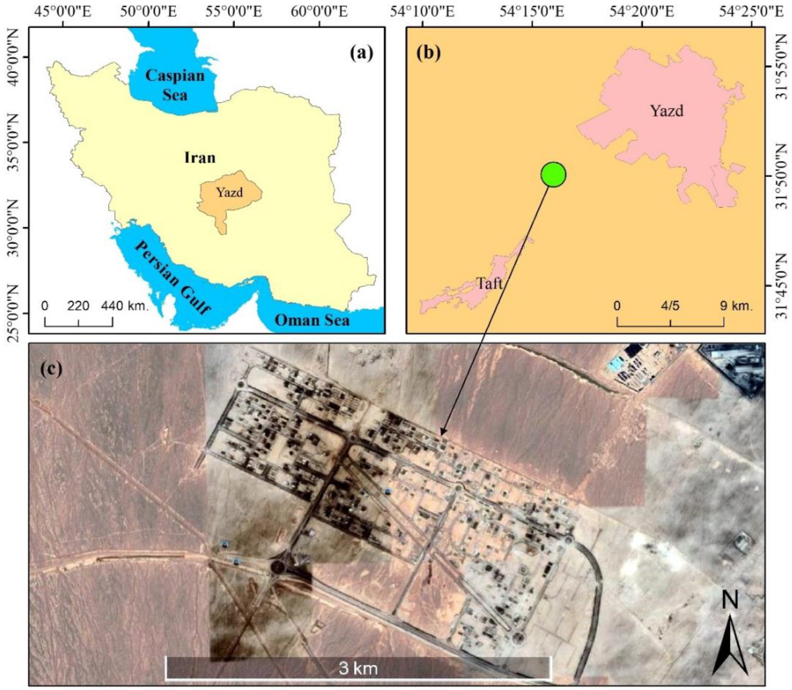
The studied area, Karizland town, is located in Yazd province, Iran, at 54°16′ (E) and 31°50′ (N), between the cities of Taft and Yazd (Figure 2). This resort town is also called Karizboom town or Kowsar town and was created with the aim of increasing the green space per capita in Yazd [30]. This region is located in the center of Iran with a hot and arid climate and lacks enough green space per capita [30]. The annual (average) temperature of this area is 20 °C. The hottest month of the year in this region is July with an average of 33 °C, followed by June and August with 31 °C [29].
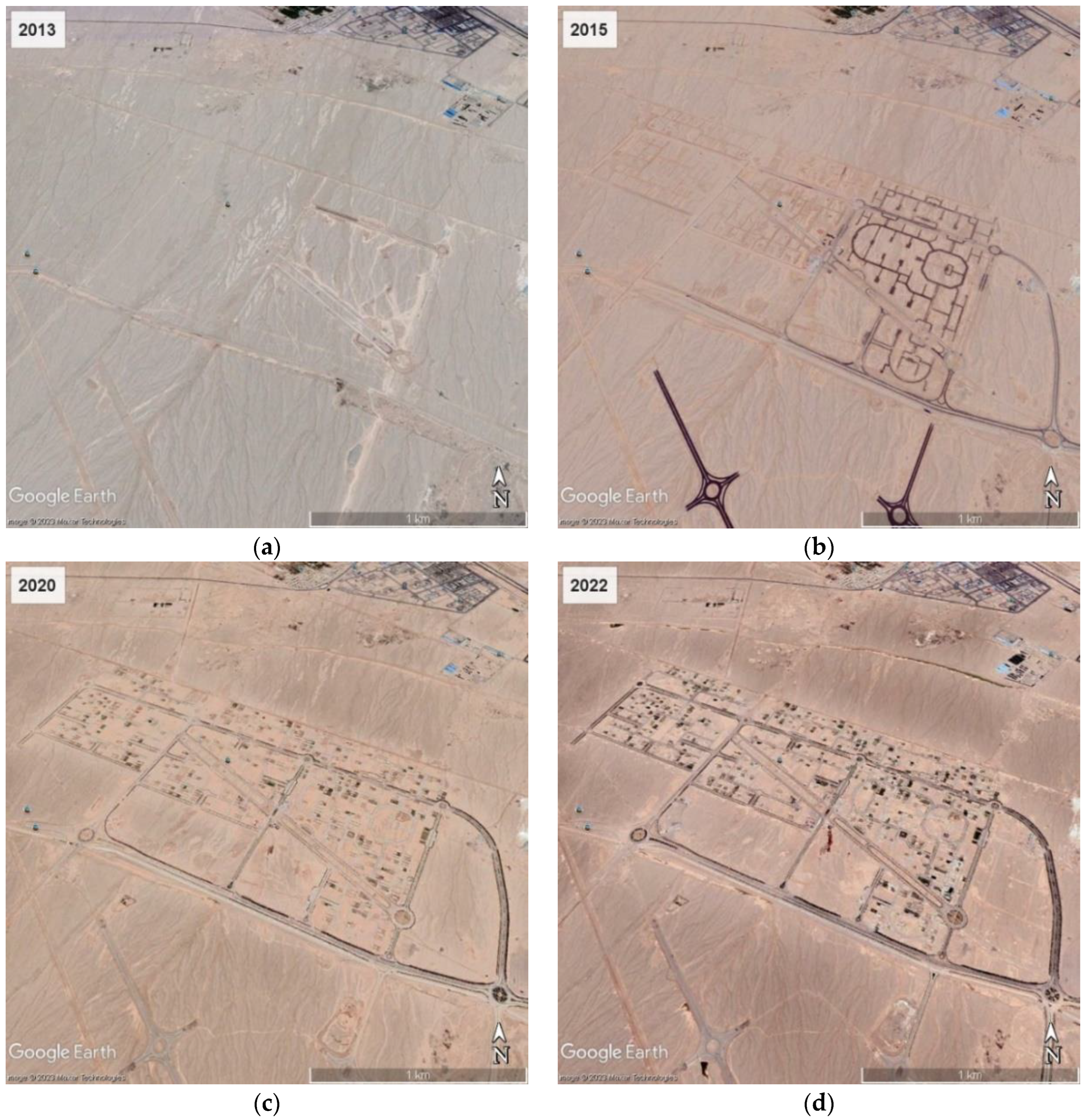
As can be seen from the Google Earth images, the construction of this town began in the beginning of 2013 (Figure 3a). Its construction was in progress in 2015 (Figure 3b) and continued until 2020 (Figure 3c). Based on this, it can be seen that part of the greening goals of this town had been achieved in 2020 and in the last quarter of 2022 (Figure 3d).

2.2. Data Collection

We used the multispectral and thermal bands of Landsat-8 Level-2 images to obtain the average values of summer vegetation cover and LST of the years 2013, 2015, 2020 and 2022 of the studied area. The reason for choosing the summer season was to establish a balance between the maximum greenness of the vegetation and the maximum LST in this area. These images were obtained from the United States Geological Survey (www.earthexplorer.usgs.gov). The characteristics of the images used are presented in Table 1.

2.3. Images Preprocessed Status and Preparation

Landsat-8 Level-2 images provide a rough approximation of the surface’s spectrum reflectance as it would be observed from the ground if air absorption or scattering did not exist. The Earth Resources Observation and Science (EROS) Center produces the surface reflectance products. Level-2 data products are produced by correcting satellite pictures for atmospheric effects using the EROS Scientific Processing Architecture (ESPA) on-demand interface. The land surface reflectance code is used to produce Landsat-8 surface reflectance data (LaSRC). LaSRC employs a special radiative transfer model, supplementary climatic data from MODIS, and the coastal aerosol band to conduct aerosol inversion experiments. Moreover, LaSRC hardcodes the view zenith angle to “0”, and computations for the atmospheric correction employ both the solar zenith and view zenith angles [32]. For the purpose of initial correction, the scale factor coefficients presented in Table 2 were applied to the images.

2.4. Calculation of Normalized Difference Vegetation Index (NDVI)

The NDVI is the ratio between the red and near-infrared bands [34,35] and is very commonly used to investigate the status of vegetation. To measure the NDVI, the leaf area index (LAI) and production pattern [36,37], which is based on vegetation class, land use/land cover changes, water stress, vegetation phenology, continental land cover mapping, and chlorophyll content [38,39,40] are usually used. According to [41], the NDVI signal from tropical evergreen woods has a poor signal-to-noise ratio because it is saturated. This is said to happen when an exponential or linear regression model is used to link the NDVI to the LAI [42]. Nevertheless, because the area under study in this article is semi-arid, this may not necessarily apply to its vegetation. In order to calculate this index, two red and near infrared bands of Landsat-8 Level-2 were used. After obtaining these images, they were multiplied by the corresponding calibration coefficients (Table 2) and then N D V I was calculated using Equation (1):
N D V I = R e d N I R R e d + N I R ,
where R e d is the 4th and the 5th band of Landsat-8.

2.5. Calculation of Fractional Vegetation Cover (FVC)

FVC is a crucial biophysical metric for studies on land surface processes, climate change, and numerical weather prediction [43,44]. It is also a crucial parameter for measuring surface vegetation cover [45]. Moreover, FVC is widely used in forestry, resource management, land use, hydrology, disaster risk assessment, and drought monitoring [20]. The FVC of the pixel is technically defined by Equation (2) as the proportional area of vegetation [20,46].
f = N D V I N D V I s N D V I v + N D V I s ,
where the subscripts N D V I s and N D V I s denote NDVI values over fully vegetated area and bare soil, respectively.

2.6. Calculation of Land Surface Temperature (LST)

In the present study, LST was calculated from surface temperature measures using emissivity correction [34,47,48,49,50,51,52,53].
L S T = τ 1 + w τ p ln e   ,
where τ is the at-sensor brightness temperature, w is the wavelength of emitted radiance (10.8 µm Landsat-8 TIRS 10th band), p = h × c / s   1.438 × 10 2 m · K , with h being the Plank’s constant ( 6.626 × 10 34 J · s ), s is the Boltzmann Constant ( 1.38 × 10 23 J / K ), c is the velocity of light ( 2.988 × 10 8 m / s ), and e is the land surface emissivity.
The land surface emissivity e was calculated using [34,47,48,49,50,52,53]:
e = n   P v + m ,
where n = 0.004 and m = 0.986, and P v denotes the vegetation proportion, also referred to as the fractional vegetation cover. The vegetation proportion ( P v ) was calculated as [34,47,48,49,50,51,52,53]:
P v = N D V I N D V I m i n N D V I m a x N D V I m i n 2 ,
where N D V I m i n and N D V I m a x are the minimal and maximal values of the NDVI.

2.7. Hot Spot Analysis

For each feature, the Getis-Ord Gi-star (G-i-*) statistic was calculated via hot spot analysis. Each characteristic was examined in the context of its nearby features in this analysis. Even a feature with a high value may not be a statistically significant hot spot. A feature must have a high value and be surrounded by additional features that have high values in order to be a statistically significant hot spot. A statistically significant z-score is produced when the local sum for a feature and its neighbors deviates significantly from the predicted local sum and deviates by an amount that is too great to be the product of random chance [54].
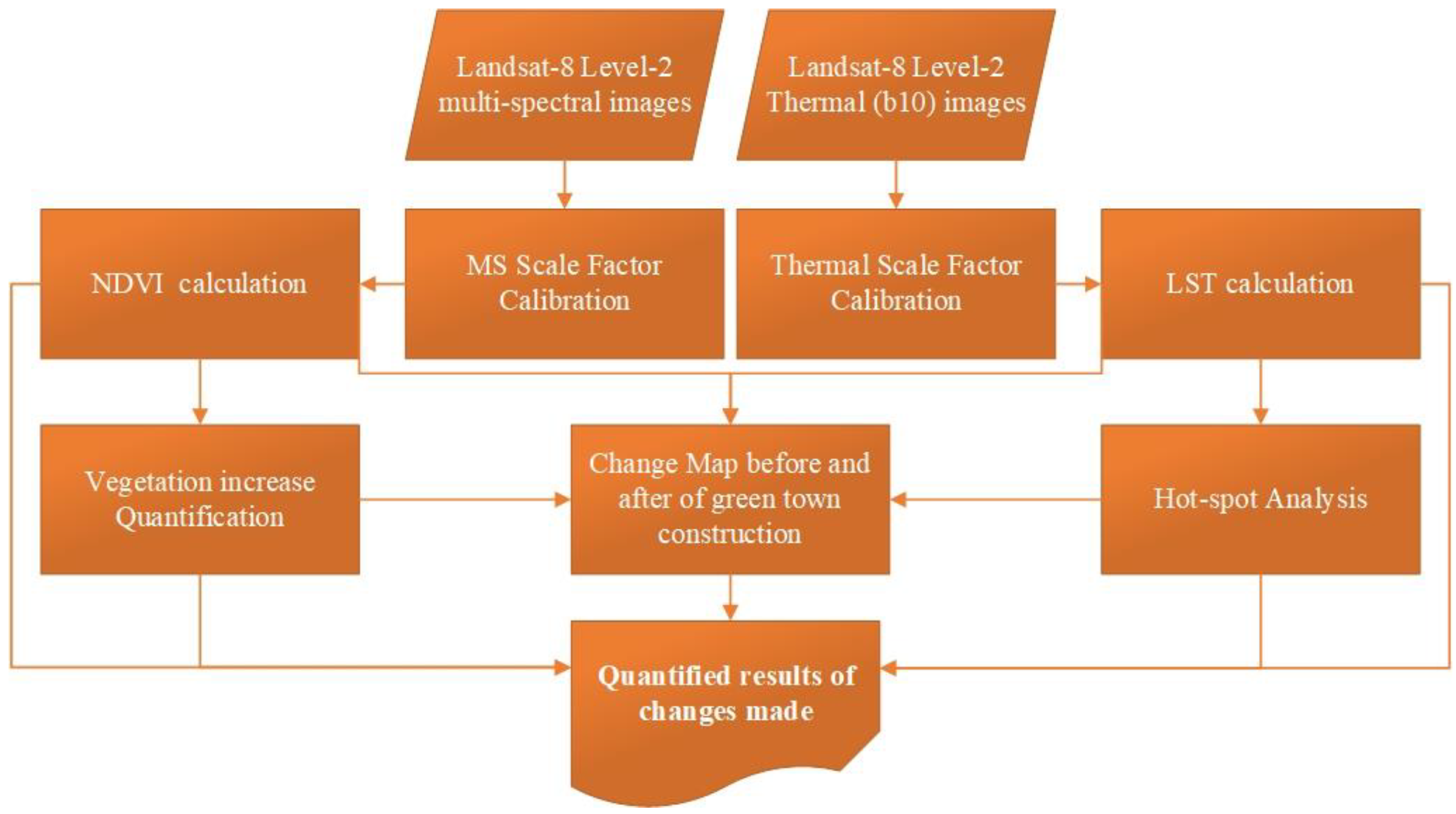
The process of conducting the research is shown in the flow chart (Figure 4).

3. Results

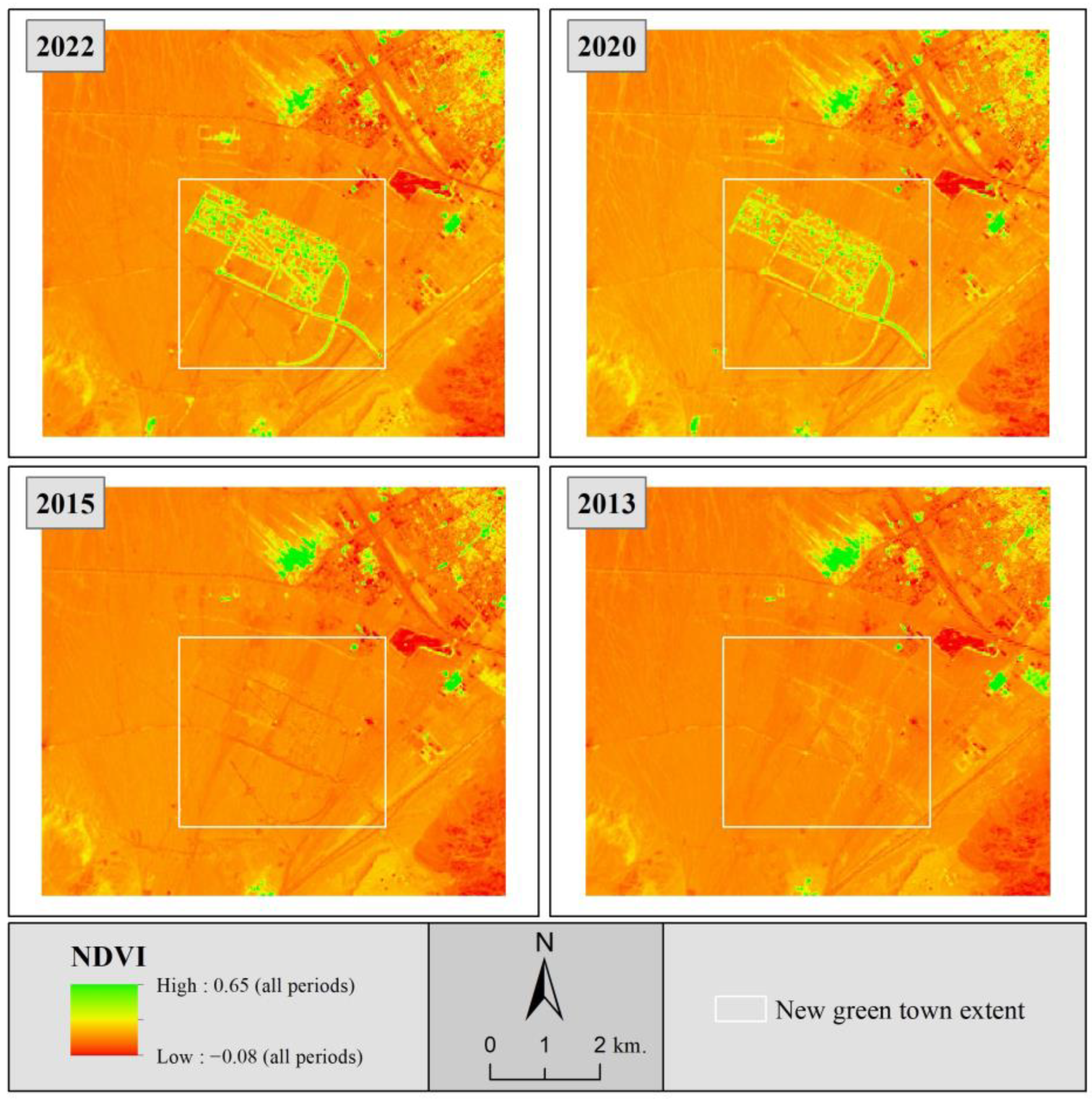
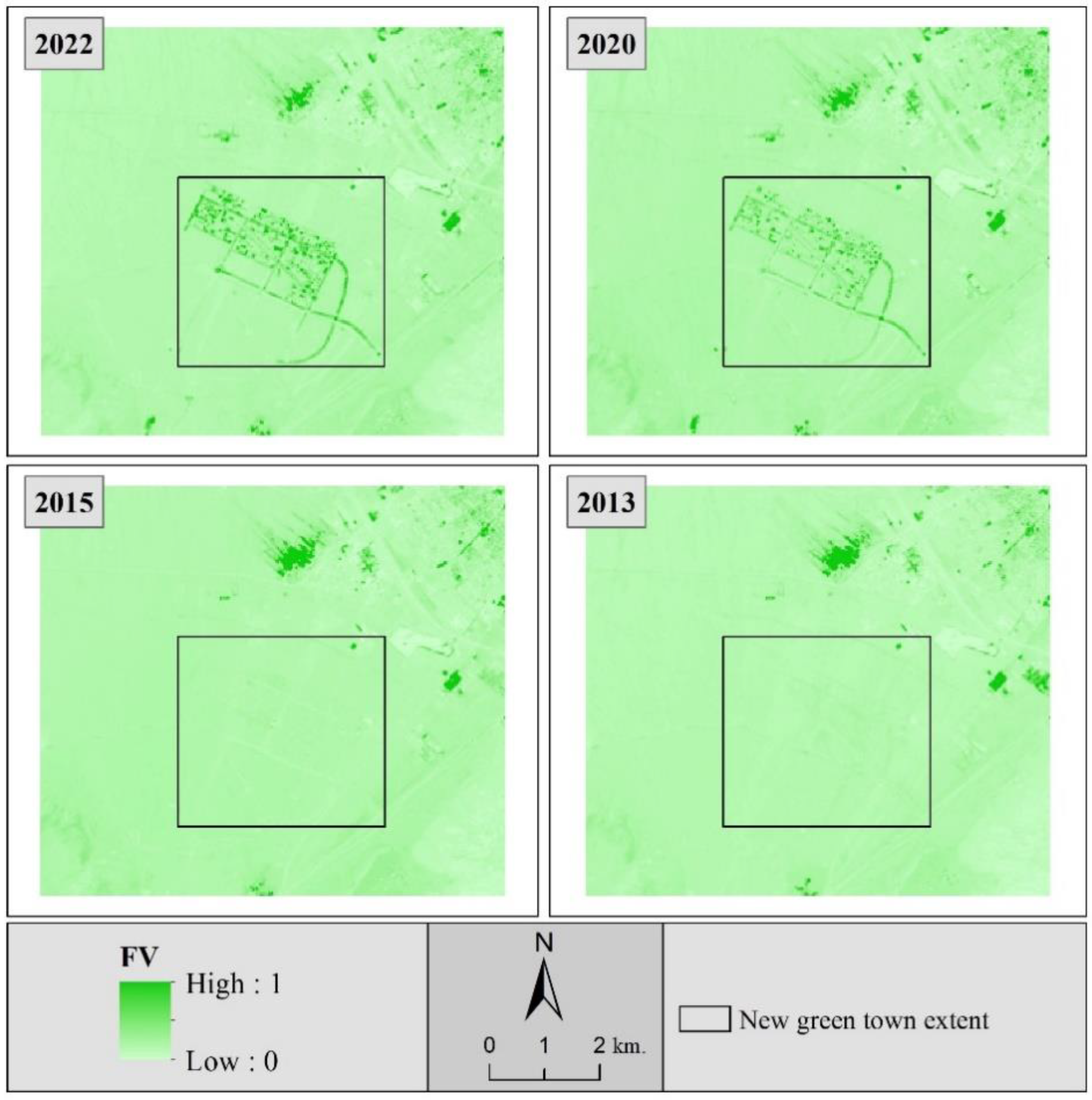
The present study was conducted in order to quantify the construction effects of the green town (green belt) of the Karizland environs of the Yazd metropolis on its peripheral area’s LST. For this purpose, in order to monitor the vegetation changes in the area, the NDVI (Figure 5) and FVC (Figure 6) map of the study area was extracted using satellite images.
The statistics of vegetation changes in the region clearly indicate an increasing trend of vegetation (Table 3). Thus, in the green zone, the NDVI minimum and maximum reached 0.12 and 0.61 in 2022 from 0.05 and 0.08 in 2013, respectively. A decrease of 0.01 is observed in the NDVI minimum and maximum in 2015. In addition, in the same period, the FVC minimum and maximum increased from 0.02 and 0.06 to 0.07 and 0.58, respectively. The NDVI and FVC means also increased from 0.12 and 0.04 to 0.45 and 0.42, respectively, with continuous growth in the three periods after 2013, i.e., 2015, 2020 and 2022. However, despite the differences, the RANGE values of 2020 compared to 2022 and 2013 compared to 2015 were very close to each other.
The vegetation changes map in the area also clearly shows the location and extent of vegetation created by the construction of Karizland green town (Figure 7). Based on these change map statistics, it is estimated that by 2022, in the new green town extent, a green belt 81,540 m long with an area equal to 208.35 ha has been created.
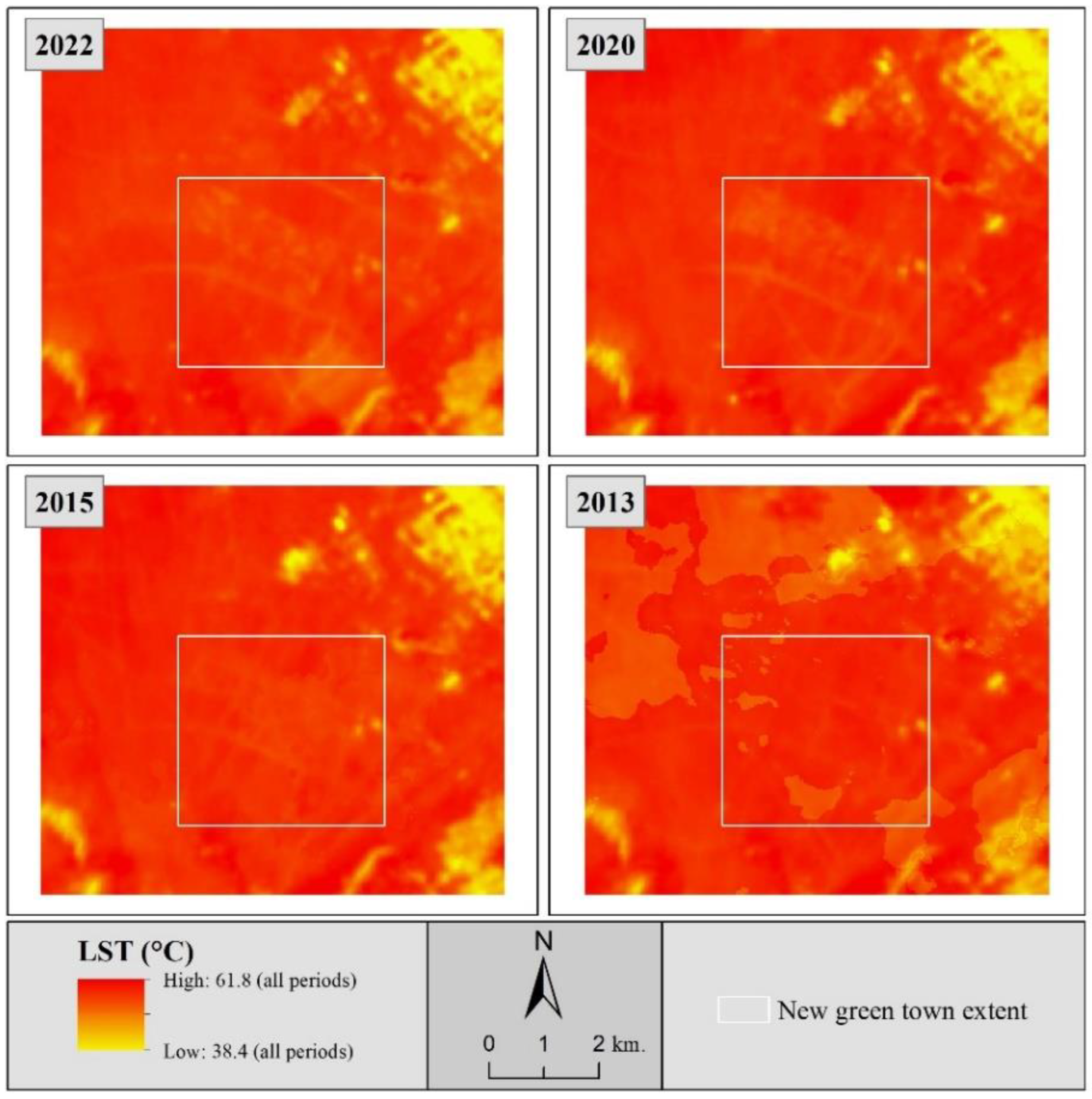
In order to investigate the LST changes before, during and after the construction of the Sabz settlement, the LST maps of the region for the studied years were extracted from the data of satellite images (Figure 8).
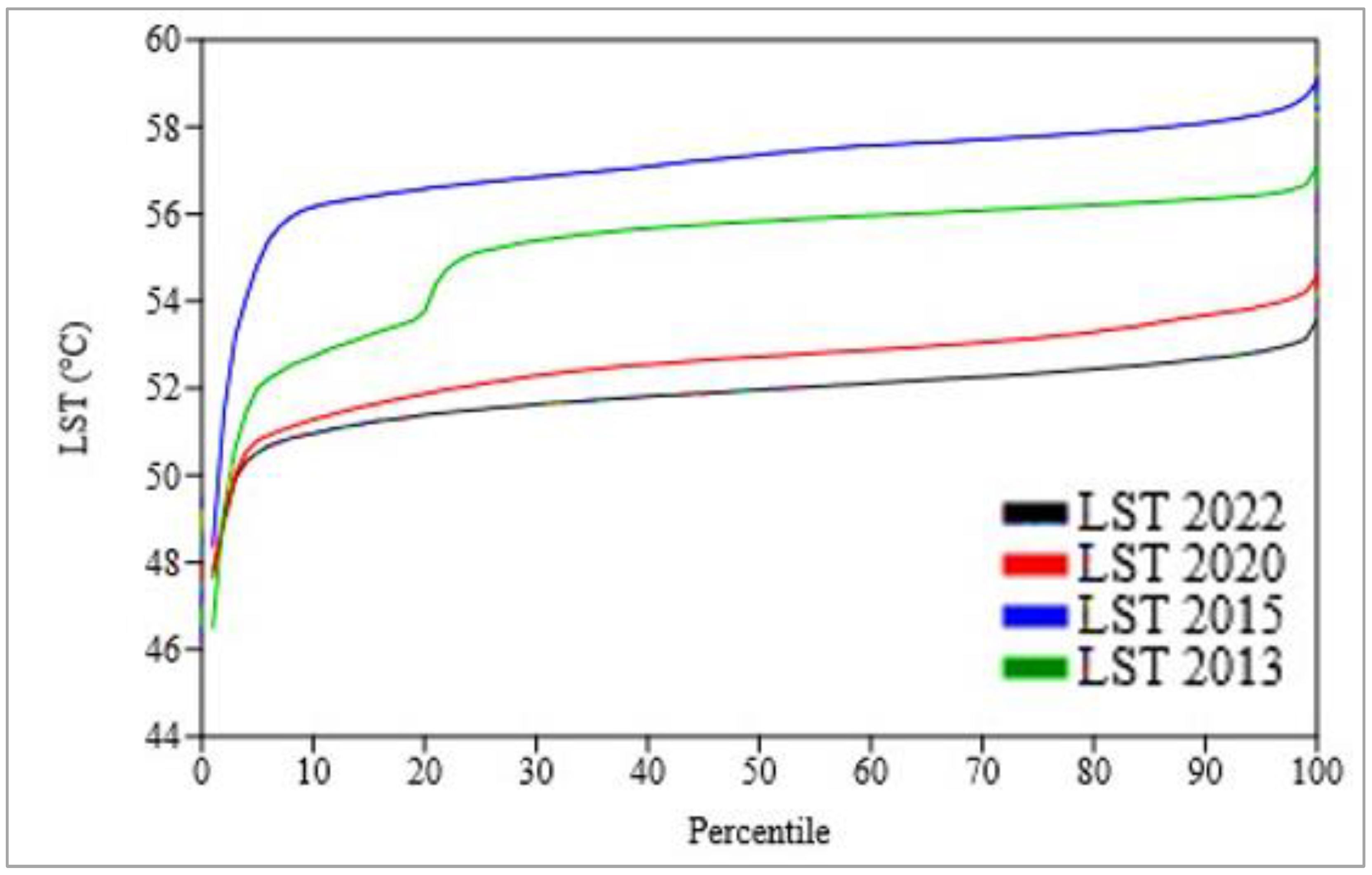
The statistics of the LST changes in the region in the four years under study show a decrease in the LST minimum and maximum of 6.9% and LST mean of 8.3% between the first and last years of the study, 2013 and 2022 (Table 4). The only visible contrast is in the thermal data of 2015, in which, when compared to 2013, the LST minimum increased by 6.6% and the maximum by 2.2%. The LST mean also increased that year, but slightly by 1.7% (less than 1 °C). Figure 9 makes it clear that the distribution of data based on percentile in the first 5% to 20% shows a lot of abnormality and change. Accordingly, in 2013, almost 20% of the data in the LST range is less than 55 °C, for 2015 it is close to 57 °C, and for 2020 and 2022 it is around 51 °C. The trend of these changes over time has mostly been related to the first 20 percentiles of LST values, while in the rest of the percentiles, the values of the two years 2013 and 2015 and the values of the two years 2020 and 2022 have been closer to each other and further away from the other group (Figure 9).
It also emerges visually from the matrix plot of LST over the time that the warmer pixels gradually decreased from 2013 to 2022 (Figure 10). This decrease started from 2015 and continued almost until 2020, so that the ratio of warmer pixels to cooler pixels reaches 50% between 2015 and 2020.
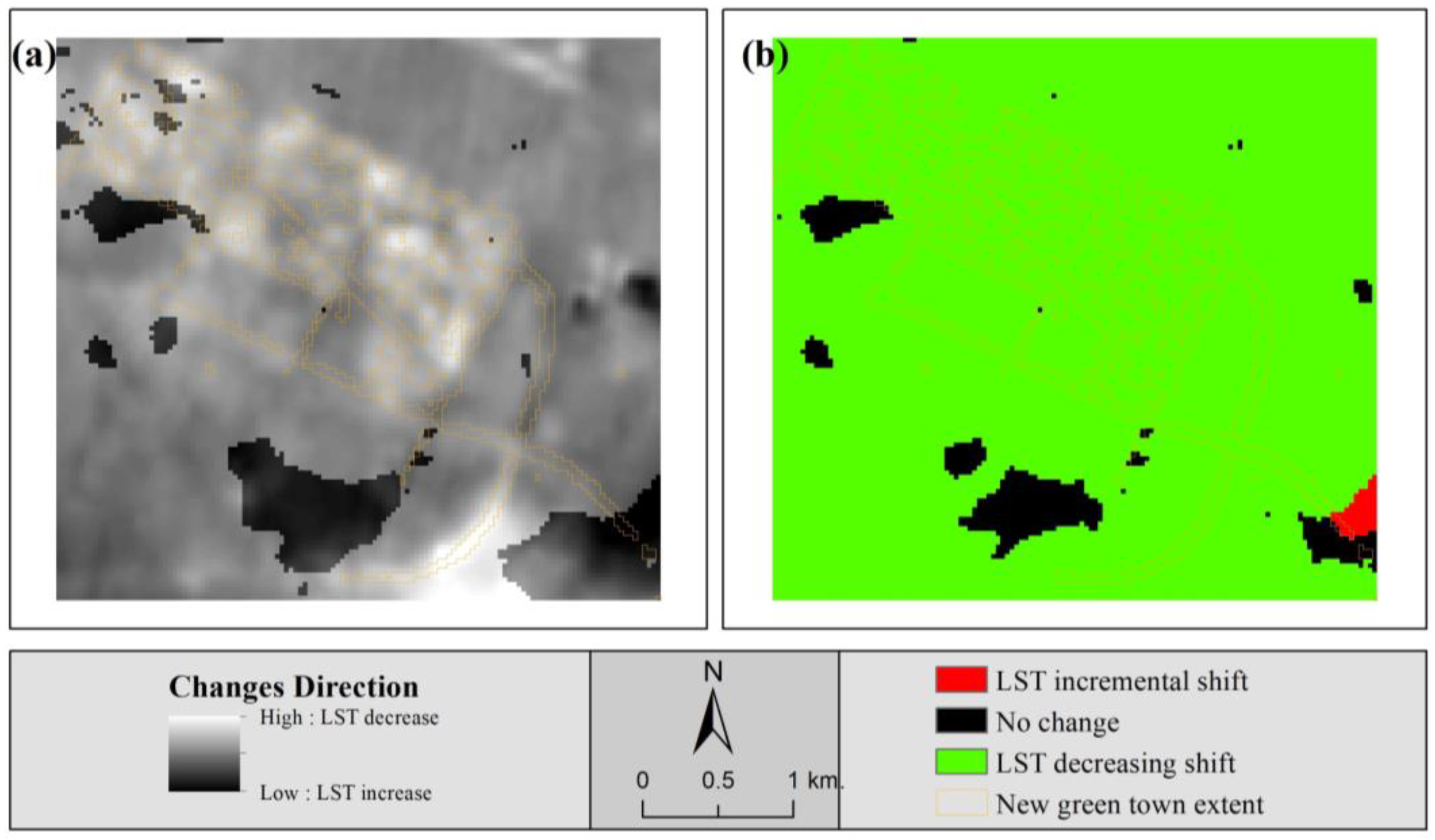
The LST difference map between 2013 and 2022 shows a clear temperature decrease in the location of the built green town and its surroundings (Figure 11). Based on this and the extent of the studied green town in 2022, 1348.2 ha of land surface had cooled, 60.66 ha had not changed and 6.84 ha of land was warmer compared to 2013.
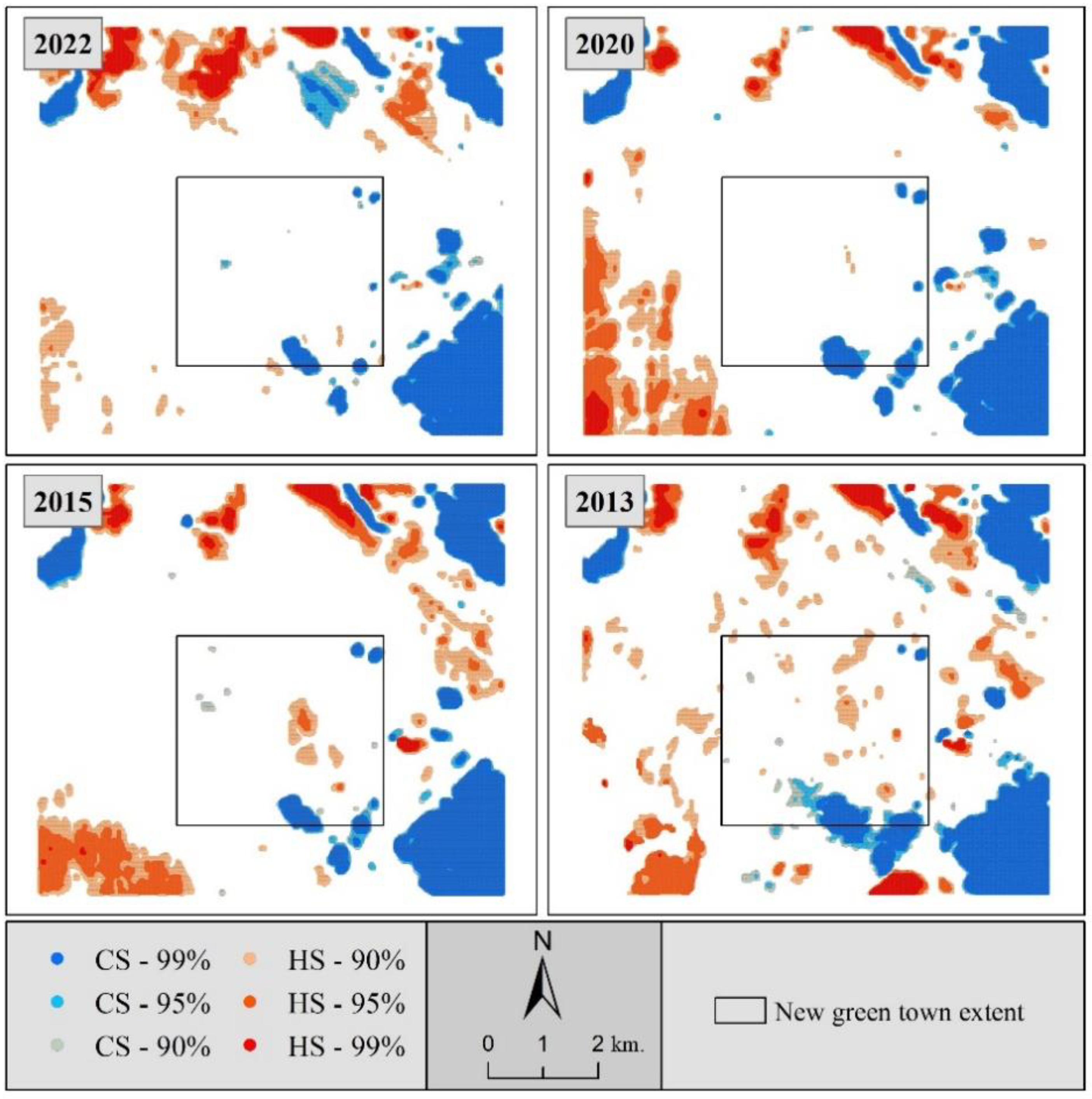
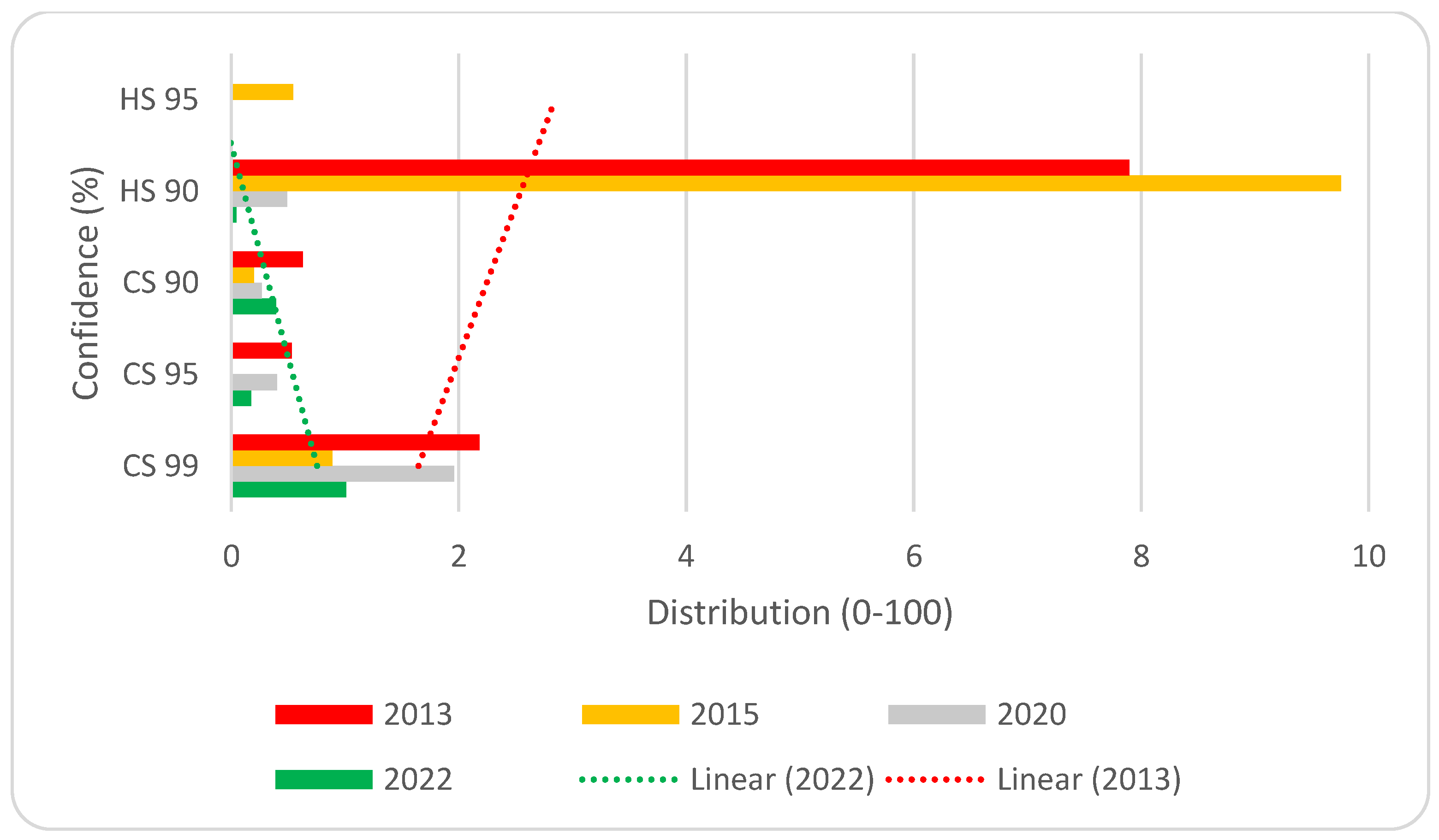
In order to investigate the status of changes in hot–cold spots, a hot spot and cold spot map was prepared for the region for the four years under study (Figure 12). The distribution investigation results of hot and cold spots in the new green town extent area show that cold spots with 99%, 95%, and 90% confidence have reached 0.99%, 0.17%, and 0.39% of the area in 2022, respectively, with a slight decrease from 1.96%, 0.48%, and 0.57% of the area in 2013. On the other hand, hot spots with 90% confidence have decreased from 7.10% of the area in 2013 to only 0.04% of the area in 2022 (Figure 13). Sharp changes have occurred in non-significant values, which covered 88.76% of the area in 2013 and 96.84% in 2022. In addition, in almost all classes except for cold spots, with 99% confidence, an increase in hot spots and a decrease in cold spots from 2013 to 2015 can be observed. As such, the largest area with hot spots with 90% confidence after 2013 was 2.5%, and the largest area with hot spots with 95% confidence was 0.39%, both belonging to 2015.
The results obtained in the correlations between the investigated parameters in the present study (Table 5) indicate that the distance from the new green town subsurface had a negative relationship of −69% with the difference between the 2022 and 2013 NDVIs. In addition, its correlation with the LSTs of 2022 and 2020 was considerable, at 61% and 50%, respectively. The correlation between distance and NDVI and FVC was negative and high in both the mentioned years, and in 2022 this negative correlation was significantly higher. The results show a negative correlation between the difference between the 2022 and 2013 NDVIs and the LSTs of 2022 and 2020, stronger for that with 2022, and a positive correlation with the NDVI in 2022. The difference in NDVIs also has a close-to-significant low correlation with the 2020 NDVI, at 48%. The correlations of the LST values of different years interestingly show a negative and high correlation with the NDVI and FVC of that year and a positive relationship with the LST values of previous years (the biggest one is the correlation between the LST in 2022 and the LST in 2020, at 90%) with a decreasing trend in following years. This trend can be seen in 2015 regarding the 2013 NDVI and FVC too. It is noteworthy that the LST values in 2022 and 2020 had high and almost identical negative correlations with the NDVIs and FVCs of the same years, with −87% and −84%, respectively. The lowest correlation of this type is in relation to 2013, with −58% and −56%, respectively. Examining the relationship between the NDVIs and FVCs for each year also shows that these values have positive and very high correlations, more than 97%, and also have positive and high correlations with the NDVIs and FVCs of each previous year. The relationship in 2020 between the NDVI and FVC values of 2013 is also significant, positive, and high.

4. Discussion

The goal of the current study was to measure the construction-related impacts of the Karizland’s green town (green belt) on the LST of its city surroundings. Based on this, using satellite images, the changes in the calculated parameters of LST, hot spots, vegetation (using NDVI and FVC) and also the connections between them were investigated. For 2013, it was seen that the average values of NDVI and FVC were very low and close to zero with 0.12 and 0.04 respectively. In this year, the RANGEs of these two indicators were 0.03 and 0.04, respectively, which seems acceptable considering the lack of vegetation and the absence of the green town in this area. The lack of vegetation in 2013 caused that year to be the second hottest year studied, with a small difference from 2015, with an average LST of 55.83 °C, as well as a high distribution of hot spots with 90% confidence, of almost 8 out of 100. In 2013, the relationship between the distance from where the green settlement would later be built and LSTs, with a rate of −56%, was close to significant (therefore unreliable) but “negative”, which probably indicates the distance of this extent from the urban environment. The hotness of this area was compared to its surroundings. The same type of relationship was seen between the LST and the NDVI and FVC values, with −58% and −56%, respectively, and despite the very low values of NDVI and FVC, the correlation was “negative”. For 2015, it was seen that the values of NDVI and FVC reached 0.14 and 0.05, respectively, with a very slight increase. According to the NDVI values, these values do not prove the presence of vegetation in the area [55,56], but at the same time, the values may be due to the activity carried out in the direction of the construction of the green town. However, the average LST increased to 56.77 °C (a 1.68% increase compared to 2013) and the distribution of hotspots in the extent reached 10 (out of 100) with 90% confidence and even more than 0.5 with 95% confidence. This increase in temperature seems reasonable considering the start of the construction of the green town according to Figure 3b, because an increase in soil excavation, road construction and other construction measures on soil causes an increase in roughness, an increase in soil emissivity, and as a result, increased LST [57] in this area. For 2015, there was no significant relationship between the LST values and the distance from the under-construction green town or the NDVI difference between 2022 and 2013, but the correlation of LST values with the 2015 NDVI and FVC values was significantly negative with −68% and −64%, respectively. However, in any case, as discussed in the above lines, due to the lack of vegetation, no effect on LST was visible. The LST values for 2015 had a positive correlation of 73% with the LST values of 2013, and this probably indicates that the pattern of LST values that year was somewhat similar to 2013, which seems reasonable considering the absence of vegetation. This can be proven due to the very high correlation of NDVI and FVC values across both 2015 and 2013. This is because, according to the negative relationship between the LST and vegetation [29,58,59,60,61,62], when there is no vegetation in the area, the LST will not change. For 2020, however, the results were that the average NDVI increased by 157% and the FVC increased by 440% compared to 2015. The RANGE changes of the NDVI values also increased from 0.03 to 0.48 (a 1500% increase), which can firstly indicate an increase in vegetation and secondly its diversity in this region in 2020. In the meantime, the 9% decrease in the average LST (reaching 51.83 °C), the increase in cold spots with 99% confidence to 2 (out of 100) and the decrease in hot spots with 90% confidence to below 0.5 in 2020 show the vegetation presence effects more clearly in this year. In 2020, finally, the correlation between the values of the distance from the green town subsurface and LST has become positive, but close to significant (unreliable). However, the correlations of distance with NDVI and FVC are negative and significant with −67% and −69%, respectively, and this is likely a proof of the presence of vegetation created by the construction of the green town. In this year, the correlation between LST and NDVI and FVC has become sharper and in a higher/negative direction with −87% and −84%, respectively, and of course, it has a positive correlation of 78% with the LST of 2015. In addition, the LST of 2020 shows a positive but close-to-significant correlation with the LST of 2013, which also helps to prove the same pattern of LST changes in all periods. In 2022, the changes were such that the average values of NDVI and FVC continued to rise and increased by 25% and 56%, respectively. This proves the growing trend of vegetation in this area. The RANGE NDVI values had a slight increase of 0.01 (2%), confirming that the maximum and minimum NDVI did not change much after 2020. However, the maximum NDVI increased by 13% compared to 2020, which could indicate an increase in greenness by 2022. In this regard, the average LST also decreased by 1% to 51.21 °C, and the distribution of cold spots with 99% confidence was 0.5 (out of 100), and cold spots with 90% confidence increased to 0.4. In 2022, the increase of spots with less than 90% confidence is noticeable, such that 98.4% of the area was in this class of values. With this difference, based on the obtained results, the areas of significant classes (hot spots and cold spots together) in the studied area in 2013, 2015, 2020 and 2022 were 10.10%, 10.22%, 3.02% and 1.60% of the total area, respectively. As a result, the areas of non-significant classes (i.e., with less than 90% confidence) were 89.90%, 89.78%, 96.98% and 98.40% respectively. Thus, according to the mean values of LST in these four years, it can be said that in this study and this region, the area of significant spot classes has a positive relationship with the mean LST and the area of the non-significant spot classes has a negative relationship with the mean LST.

5. Conclusions

The present study was conducted with the aim of quantifying the effects of the construction of Karizland (Karizboom) green town on the surrounding LST for 2013 (as a year without the town), 2015 (the year that the town was being built), and 2020 and 2022 (years in which the town had been competed and with different levels of vegetation). For this purpose, using Landsat-8 satellite images, LST values and hot spot analysis were used for thermal studies, as well as NDVI and FVC indices for vegetation change studies. The obtained results indicate an increase of 81,540 m and 208.35 ha of vegetation after the establishment of the green settlement and as a result a decrease of 9.8% in LST in the period from the start to the end of the study period. Accordingly, based on the findings of this study, which were meticulously derived using maps and statistics of the cooling process of the town’s extent during the studied period, this study firmly encourages managers to create these green towns in order to control LST and the temperature around cities. The current study focused in particular on a hot and arid region in the center of Iran, thus from this perspective, the development of settlements in these areas may be significantly more important. Future studies may quantify the cooling effects of this settlement by focusing on the location of other settlements in nearby areas or in other hot and dry areas, in order to provide scientific evidence to policy makers on how to reduce temperature and improve climatic conditions. In addition, maybe the use of other vegetation indicators (like the enhanced vegetation index (EVI)) in this area to evaluate the results of this study and more detailed investigations focusing on the vegetation approach will provide room for further studies.

Author Contributions

Conceptualization, M.M. and I.R.; methodology, M.M.; software, M.M. and N.N.; validation, M.M., I.R., S.K.A. and H.O.; formal analysis, M.M. and I.R.; investigation, M.M.; resources, M.M. and N.N.; data curation, M.M., N.N. and I.R.; writing—original draft preparation, M.M. and N.N.; writing—review and editing, M.M., N.N., I.R. and A.A.A.; visualization, M.M.; supervision, I.R., S.K.A. and H.O.; project administration, M.M. and I.R.; funding acquisition, I.R. and A.A.A. All authors have read and agreed to the published version of the manuscript.

Funding

This research received no external funding.

Data Availability Statement

Acknowledgments

The authors are grateful to; 1- Vedurfelagid, Rannis and Rannsoknastofai vedurfraedi-Iceland, and 2- Shanghai Municipal Science and Technology Commission within the international cooperation framework of the Youth Scientists from the ‘One Belt and One Road’ countries (2020–2023) for their supports.

Conflicts of Interest

The authors declare no conflict of interest.

References

  1. Simonds, J.O. Landscape Architecture: A Manual of Site Planning and Design; McGraw-Hill Professional: New York, NY, USA, 1997. [Google Scholar]
  2. Tong, D.; Chu, J.; Han, Q.; Liu, X. How land finance drives urban expansion under fiscal pressure: Evidence from Chinese cities. Land 2022, 11, 253. [Google Scholar] [CrossRef]
  3. Liu, X.; Kong, M.; Tong, D.; Zeng, X.; Lai, Y. Property rights and adjustment for sustainable development during post-productivist transitions in China. Land Use Policy 2022, 122, 106379. [Google Scholar] [CrossRef]
  4. Alavipanah, S.K. Thermal Remote Sensing and Its Application in the Earth Sciences; University of Tehran press: Tehran, Iran, 2006; pp. 903–964. [Google Scholar]
  5. Kazemi Garajeh, M.; Salmani, B.; Zare Naghadehi, S.; Valipoori Goodarzi, H.; Khasraei, A. An integrated approach of remote sensing and geospatial analysis for modeling and predicting the impacts of climate change on food security. Sci. Rep. 2023, 13, 1057. [Google Scholar] [CrossRef] [PubMed]
  6. Wang, P.; Yu, P.; Lu, J.; Zhang, Y. The mediation effect of land surface temperature in the relationship between land use-cover change and energy consumption under seasonal variations. J. Clean. Prod. 2022, 340, 130804. [Google Scholar] [CrossRef]
  7. Şimşek, Ç.K.; Ödül, H. A method proposal for monitoring the microclimatic change in an urban area. Sustain. Cities Soc. 2019, 46, 101407. [Google Scholar] [CrossRef]
  8. Liu, L.; Li, Z.; Fu, X.; Liu, X.; Li, Z.; Zheng, W. Impact of power on uneven development: Evaluating built-up area changes in Chengdu based on NPP-VIIRS images (2015–2019). Land 2022, 11, 489. [Google Scholar] [CrossRef]
  9. Meng, H.; Jing, L.; Xin, H. The influence of underlying surface on land surface temperature—A case study of urban green space in Harbin. Energy Procedia 2019, 157, 746–751. [Google Scholar]
  10. He, F.; Mohamadzadeh, N.; Sadeghnejad, M.; Ingram, B.; Ostovari, Y. Fractal Features of Soil Particles as an Index of Land Degradation under Different Land-Use Patterns and Slope-Aspects. Land 2023, 12, 615. [Google Scholar] [CrossRef]
  11. Temme, A.; Sadeghnejad, M.; Sodhi, H.S.; Samia, J. Search for Path-Dependency Mechanisms Using Physically-Based Soil-Landscape Modelling of Landslides. In Proceedings of the Copernicus Meetings, Vienna, Austria, 24–28 April 2023. [Google Scholar]
  12. Gorse, C.; Parker, J.; Thomas, F.; Fletcher, M.; Ferrier, G.; Ryan, N. The Planning and Design of Buildings: Urban Heat Islands—Mitigation. In Industry 4.0 and Engineering for a Sustainable Future; Springer: Berlin/Heidelberg, Germany, 2019; pp. 211–225. [Google Scholar]
  13. Yahia, M.W.; Johansson, E.; Thorsson, S.; Lindberg, F.; Rasmussen, M.I. Effect of urban design on microclimate and thermal comfort outdoors in warm-humid Dar es Salaam, Tanzania. Int. J. Biometeorol. 2018, 62, 373–385. [Google Scholar] [CrossRef] [Green Version]
  14. Wolch, J.R.; Byrne, J.; Newell, J.P. Urban green space, public health, and environmental justice: The challenge of making cities ‘just green enough’. Landsc. Urban Plan. 2014, 125, 234–244. [Google Scholar] [CrossRef] [Green Version]
  15. Shang, Y.; Lian, Y.; Chen, H.; Qian, F. The impacts of energy resource and tourism on green growth: Evidence from Asian economies. Resour. Policy 2023, 81, 103359. [Google Scholar] [CrossRef]
  16. Yang, J.; Sun, J.; Ge, Q.; Li, X. Assessing the impacts of urbanization-associated green space on urban land surface temperature: A case study of Dalian, China. Urban For. Urban Green. 2017, 22, 1–10. [Google Scholar] [CrossRef]
  17. Zölch, T.; Maderspacher, J.; Wamsler, C.; Pauleit, S. Using green infrastructure for urban climate-proofing: An evaluation of heat mitigation measures at the micro-scale. Urban For. Urban Green. 2016, 20, 305–316. [Google Scholar] [CrossRef]
  18. Kazemi Garajeh, M.; Li, Z.; Hasanlu, S.; Zare Naghadehi, S.; Hossein Haghi, V. Developing an integrated approach based on geographic object-based image analysis and convolutional neural network for volcanic and glacial landforms mapping. Sci. Rep. 2022, 12, 21396. [Google Scholar] [CrossRef]
  19. Rothery, D.; Francis, P.; Wood, C. Volcano monitoring using short wavelength infrared data from satellites. J. Geophys. Res. Solid Earth 1988, 93, 7993–8008. [Google Scholar] [CrossRef]
  20. Liang, S.; Wang, J. Advanced Remote Sensing: Terrestrial Information Extraction and Applications; Academic Press: Cambridge, MA, USA, 2020; Volume 2. [Google Scholar]
  21. Zare Naghadehi, S.; Asadi, M.; Maleki, M.; Tavakkoli-Sabour, S.-M.; Van Genderen, J.L.; Saleh, S.-S. Prediction of Urban Area Expansion with Implementation of MLC, SAM and SVMs’ Classifiers Incorporating Artificial Neural Network Using Landsat Data. ISPRS Int. J. Geo-Inf. 2021, 10, 513. [Google Scholar] [CrossRef]
  22. Amani-Beni, M.; Zhang, B.; Xie, G.-D.; Shi, Y. Impacts of urban green landscape patterns on land surface temperature: Evidence from the adjacent area of Olympic Forest Park of Beijing, China. Sustainability 2019, 11, 513. [Google Scholar] [CrossRef] [Green Version]
  23. Sun, S.; Xu, X.; Lao, Z.; Liu, W.; Li, Z.; García, E.H.; He, L.; Zhu, J. Evaluating the impact of urban green space and landscape design parameters on thermal comfort in hot summer by numerical simulation. Build. Environ. 2017, 123, 277–288. [Google Scholar] [CrossRef]
  24. Zhao, L.; Du, M.; Du, W.; Guo, J.; Liao, Z.; Kang, X.; Liu, Q. Evaluation of the Carbon Sink Capacity of the Proposed Kunlun Mountain National Park. Int. J. Environ. Res. Public Health 2022, 19, 9887. [Google Scholar] [CrossRef] [PubMed]
  25. Bai, X.; Zhang, S.; Li, C.; Xiong, L.; Song, F.; Du, C.; Li, M.; Luo, Q.; Xue, Y.; Wang, S. A carbon neutrality capacity index for evaluating carbon sink contributions. Environ. Sci. Ecotechnol. 2023, 15, 100237. [Google Scholar] [CrossRef]
  26. Di Leo, N.; Escobedo, F.J.; Dubbeling, M. The role of urban green infrastructure in mitigating land surface temperature in Bobo-Dioulasso, Burkina Faso. Environ. Dev. Sustain. 2016, 18, 373–392. [Google Scholar] [CrossRef] [Green Version]
  27. Li, X.; Zhang, X.; Jia, T. Humanization of nature: Testing the influences of urban park characteristics and psychological factors on collegers’ perceived restoration. Urban For. Urban Green. 2023, 79, 127806. [Google Scholar] [CrossRef]
  28. Jiang, J.; Tian, G. Analysis of the impact of land use/land cover change on land surface temperature with remote sensing. Procedia Environ. Sci. 2010, 2, 571–575. [Google Scholar] [CrossRef] [Green Version]
  29. Mansourmoghaddam, M.; Rousta, I.; Zamani, M.; Mokhtari, M.H.; Karimi Firozjaei, M.; Alavipanah, S.K. Study and prediction of land surface temperature changes of Yazd city: Assessing the proximity and changes of land cover. J. RS GIS Nat. Resour. 2021, 12, 1–27. [Google Scholar]
  30. Ettelaat. “Karizland” Becomes the Green Gem of Yazd Province. Available online: https://www.ettelaat.com/mobile/archives/130034?device=phone (accessed on 26 February 2023). (In Persian).
  31. Kowsar Institute. The Return of Freshness, Freshness and Greenery to KARIZBOOM after Water Stress. Available online: https://portal.kowsaryazd.com/anounce/ (accessed on 27 February 2023).
  32. USGS. USGS EROS Archive—Landsat Archives—Landsat 8 OLI/TIRS Level-2 Data Products—Surface Reflectance. Available online: https://www.usgs.gov/centers/eros/science/usgs-eros-archive-landsat-archives-landsat-8-olitirs-level-2-data-products (accessed on 27 February 2023).
  33. USGS. Landsat Collection 2 Level-2 Science Products. Available online: https://www.usgs.gov/landsat-missions/landsat-collection-2-level-2-science-products (accessed on 27 February 2023).
  34. Avdan, U.; Jovanovska, G. Algorithm for automated mapping of land surface temperature using LANDSAT 8 satellite data. J. Sens. 2016, 2016, 1480307. [Google Scholar] [CrossRef] [Green Version]
  35. Li, X.; Zhou, Y.; Asrar, G.R.; Imhoff, M.; Li, X. The surface urban heat island response to urban expansion: A panel analysis for the conterminous United States. Sci. Total Environ. 2017, 605, 426–435. [Google Scholar] [CrossRef]
  36. Dutta, D.; Kundu, A.; Patel, N.; Saha, S.; Siddiqui, A. Assessment of agricultural drought in Rajasthan (India) using remote sensing derived Vegetation Condition Index (VCI) and Standardized Precipitation Index (SPI). Egypt. J. Remote Sens. Space Sci. 2015, 18, 53–63. [Google Scholar] [CrossRef] [Green Version]
  37. Tarpley, J.; Schneider, S.; Money, R. Global vegetation indices from the NOAA-7 meteorological satellite. J. Clim. Appl. Meteorol. 1984, 23, 491–494. [Google Scholar] [CrossRef]
  38. Moulin, S.; Kergoat, L.; Viovy, N.; Dedieu, G. Global-scale assessment of vegetation phenology using NOAA/AVHRR satellite measurements. J. Clim. 1997, 10, 1154–1170. [Google Scholar] [CrossRef]
  39. Running, S.W.; Loveland, T.R.; Pierce, L.L.; Nemani, R.R.; Hunt, E.R., Jr. A remote sensing based vegetation classification logic for global land cover analysis. Remote Sens. Environ. 1995, 51, 39–48. [Google Scholar] [CrossRef]
  40. Townshend, J.R.; Justice, C. Analysis of the dynamics of African vegetation using the normalized difference vegetation index. Int. J. Remote Sens. 1986, 7, 1435–1445. [Google Scholar] [CrossRef]
  41. Schlerf, M.; Atzberger, C.; Hill, J. Remote sensing of forest biophysical variables using HyMap imaging spectrometer data. Remote Sens. Environ. 2005, 95, 177–194. [Google Scholar] [CrossRef] [Green Version]
  42. Yengoh, G.T.; Dent, D.; Olsson, L.; Tengberg, A.E.; Tucker, C.J., III. Use of the Normalized Difference Vegetation Index (NDVI) to Assess Land Degradation at Multiple Scales: Current Status, Future Trends, and Practical Considerations; Springer: Berlin/Heidelberg, Germany, 2015. [Google Scholar]
  43. Wei, Q.; Qingke, Z.; Xuexia, Z. Review of vegetation covering and its measuring and calculating method. J. Northwest Sci-Tech Univ. Agric. For. 2006, 34, 163–170. [Google Scholar]
  44. Yin, J.; Zhan, X.; Zheng, Y.; Hain, C.R.; Ek, M.; Wen, J.; Fang, L.; Liu, J. Improving Noah land surface model performance using near real time surface albedo and green vegetation fraction. Agric. For. Meteorol. 2016, 218, 171–183. [Google Scholar] [CrossRef]
  45. Zeng, X.; Dickinson, R.E.; Walker, A.; Shaikh, M.; DeFries, R.S.; Qi, J. Derivation and evaluation of global 1-km fractional vegetation cover data for land modeling. J. Appl. Meteorol. 2000, 39, 826–839. [Google Scholar] [CrossRef]
  46. Gutman, G.; Ignatov, A. The derivation of the green vegetation fraction from NOAA/AVHRR data for use in numerical weather prediction models. Int. J. Remote Sens. 1998, 19, 1533–1543. [Google Scholar] [CrossRef]
  47. Ranagalage, M.; Estoque, R.C.; Handayani, H.H.; Zhang, X.; Morimoto, T.; Tadono, T.; Murayama, Y. Relation between urban volume and land surface temperature: A comparative study of planned and traditional cities in Japan. Sustainability 2018, 10, 2366. [Google Scholar] [CrossRef] [Green Version]
  48. Bokaie, M.; Zarkesh, M.K.; Arasteh, P.D.; Hosseini, A. Assessment of urban heat island based on the relationship between land surface temperature and land use/land cover in Tehran. Sustain. Cities Soc. 2016, 23, 94–104. [Google Scholar] [CrossRef]
  49. Dos Santos, A.R.; de Oliveira, F.S.; da Silva, A.G.; Gleriani, J.M.; Gonçalves, W.; Moreira, G.L.; Silva, F.G.; Branco, E.R.F.; Moura, M.M.; da Silva, R.G. Spatial and temporal distribution of urban heat islands. Sci. Total Environ. 2017, 605, 946–956. [Google Scholar] [CrossRef]
  50. Estoque, R.C.; Pontius, R.G., Jr.; Murayama, Y.; Hou, H.; Thapa, R.B.; Lasco, R.D.; Villar, M.A. Simultaneous comparison and assessment of eight remotely sensed maps of Philippine forests. Int. J. Appl. Earth Obs. Geoinf. 2018, 67, 123–134. [Google Scholar] [CrossRef]
  51. Sultana, S.; Satyanarayana, A. Urban heat island intensity during winter over metropolitan cities of India using remote-sensing techniques: Impact of urbanization. Int. J. Remote Sens. 2018, 39, 6692–6730. [Google Scholar] [CrossRef]
  52. Ziaul, S.; Pal, S. Image based surface temperature extraction and trend detection in an urban area of West Bengal, India. J. Environ. Geogr. 2016, 9, 13–25. [Google Scholar] [CrossRef] [Green Version]
  53. Rousta, I.; Sarif, M.O.; Gupta, R.D.; Olafsson, H.; Ranagalage, M.; Murayama, Y.; Zhang, H.; Mushore, T.D. Spatiotemporal analysis of land use/land cover and its effects on surface urban heat island using Landsat data: A case study of Metropolitan City Tehran (1988–2018). Sustainability 2018, 10, 4433. [Google Scholar] [CrossRef] [Green Version]
  54. Esri. How Hot Spot Analysis (Getis-Ord Gi*) Works. Available online: https://pro.arcgis.com/en/pro-app/latest/tool-reference/spatial-statistics/h-how-hot-spot-analysis-getis-ord-gi-spatial-stati.htm#:~:text=The%20Hot%20Spot%20Analysis%20tool,the%20context%20of%20neighboring%20features (accessed on 4 March 2022).
  55. Akbar, T.A.; Hassan, Q.K.; Ishaq, S.; Batool, M.; Butt, H.J.; Jabbar, H. Investigative spatial distribution and modelling of existing and future urban land changes and its impact on urbanization and economy. Remote Sens. 2019, 11, 105. [Google Scholar] [CrossRef] [Green Version]
  56. Mansourmoghaddam, M.; Rousta, I.; Ghafarian Malamiri, H. Evaluation of the classification accuracy of NDVI index in the preparation of land cover map. Desert 2022, 27, 329–341. [Google Scholar]
  57. Shati, A.; Blakey, S.; Beck, S. The effect of surface roughness and emissivity on radiator output. Energy Build. 2011, 43, 400–406. [Google Scholar] [CrossRef]
  58. Gorgani, S.A.; Panahi, M.; Rezaie, F. The Relationship between NDVI and LST in the urban area of Mashhad, Iran. In Proceedings of the International Conference on Civil Engineering Architecture & Urban Sustainable Development, Tabriz, Iran, 27–28 November 2013; p. 51. [Google Scholar]
  59. Malik, M.S.; Shukla, J.P.; Mishra, S. Relationship of LST, NDBI and NDVI Using Landsat-8 Data in Kandaihimmat Watershed, Hoshangabad, India; NISCAIR-CSIR: Hoshangabad, India, 2019. [Google Scholar]
  60. Sun, D.; Kafatos, M. Note on the NDVI-LST relationship and the use of temperature-related drought indices over North America. Geophys. Res. Lett. 2007, 34, L24406. [Google Scholar] [CrossRef] [Green Version]
  61. Karnieli, A.; Agam, N.; Pinker, R.T.; Anderson, M.; Imhoff, M.L.; Gutman, G.G.; Panov, N.; Goldberg, A. Use of NDVI and land surface temperature for drought assessment: Merits and limitations. J. Clim. 2010, 23, 618–633. [Google Scholar] [CrossRef]
  62. Fatemi, M.; Narangifard, M. Monitoring LULC changes and its impact on the LST and NDVI in District 1 of Shiraz City. Arab. J. Geosci. 2019, 12, 127. [Google Scholar] [CrossRef]
Figure 1. A photo of parts of the green space of Karizland [31].
Land 12 00885 g001
Figure 2. The location of the studied area in Yazd province and Iran (a), its location in between Yazd city and Taft city (b), and its 2023 Google Earth image (c).
Land 12 00885 g002
Figure 3. Google Earth images of Karizland town in 2013 (a), 2015 (b), 2020 (c), and 2022 (d), which show the stages of establishing the town.
Land 12 00885 g003
Figure 4. Flowchart of the research process of the present study.
Land 12 00885 g004
Figure 5. Normalized difference vegetation index (NDVI) maps for 2013, 2015, 2020 and 2022.
Land 12 00885 g005
Figure 6. Fractional vegetation cover (FVC) maps of the studied area for 2013, 2015, 2020 and 2022.
Land 12 00885 g006
Figure 7. The difference in normalized difference vegetation index (NDVI) values in the study area between 2022 and 2013 in two representations of continuous values (a) and discrete classes (b).
Land 12 00885 g007
Figure 8. Land surface temperature (LST) maps of the studied area for 2013, 2015, 2020 and 2022.
Land 12 00885 g008
Figure 9. The trend of land surface temperature (LST) value changes in 10 percentiles according to the studied years.
Land 12 00885 g009
Figure 10. Matrix plot of land surface Temperature (LST) changes in the studied area (15,730 pixels) during the years 2013, 2015, 2020 and 2022 (masked by the built green town extent).
Land 12 00885 g010
Figure 11. The difference in land surface temperature (LST) values between 2022 and 2013 in two representations of continuous values (a) and discrete classes (b).
Land 12 00885 g011
Figure 12. Hot spot (HS) and cold spot (CS) maps of the studied area for 2013, 2015, 2020 and 2022.
Land 12 00885 g012
Figure 13. Normalized (0–100) distribution pattern of hot spot (HS) and cold spot (CS) values in the study area according to the studied years along with the trend line of changes in 2013 and 2022. Because the non-significant spots were in the majority in each year, they were 100 and were masked for chart better visibility.
Land 12 00885 g013
Table 1. Characteristics of the images used in the present study.
SatelliteSensorDate
(Year & Months)
No of
Bands Used
Spatial
Resolution
Cloud Cover (%)
Landsat-8OLI2013064, 530≤15
07
08
09
201506
07
08
09
TIRS20200610100
07
08
09
202206
07
08
09
Table 2. Scaling Factor of Level-2 Landsat-8 images [33].
Data TypeScaling Factor
Surface Reflectance0.0000275 + −0.2
Surface Temperature0.00341802 + 149.0
Table 3. Statistics (masked by the built green town subsurface) of the normalized difference vegetation index (NDVI) and fractional vegetation cover (FVC) changes according to the studied years.
NDVIFVC
YearMINMAXRANGEMEANMINMAXRANGEMEAN
20220.120.610.490.450.070.580.510.42
20200.060.540.480.360.030.360.320.27
20150.040.070.030.140.030.090.060.05
20130.050.080.030.120.020.060.040.04
Table 4. Statistics (masked by the built green town subsurface) of land surface temperature (LST) changes according to the studied years.
YearMINMAXRANGEMEAN
202248.5252.834.3251.21
202050.1953.443.2651.83
201555.5458.022.4856.77
201352.1256.774.6655.83
Table 5. The results of correlation calculations between distance from the study area, difference in normalized difference vegetation index (NDVI Diff.) between 2013 and 2022, land surface temperature (LST), NDVI, and fractional vegetation cover (FVC) for 2022, 2020, 2015 and 2013 (highlights significance: red: ≥60% and significant, yellow: ≤−60% and significant, and grey: ±50% and almost significant).
DistanceNDVI
Diff.
LST
2022
NDVI
2022
FVC
2022
LST
2020
NDVI
2020
FVC
2020
LST
2015
NDVI
2015
FVC
2015
LST
2013
NDVI
2013
NDVI
Diff.
−0.691
LST
2022
0.61−0.641
NDVI
2022
−0.910.58−0.871
FVC
2022
−0.890.38−0.840.971
LST
2020
0.50−0.560.90−0.42−0.401
NDVI
2020
−0.670.48−0.410.900.89−0.871
FVC
2020
−0.690.37−0.400.850.88−0.840.971
LST
2015
0.38−0.080.74−0.40−0.420.78−0.49−0.521
NDVI
2015
−0.060.01−0.320.510.54−0.330.680.73−0.681
FVC
2015
−0.060.00−0.300.470.53−0.300.640.72−0.640.981
LST
2013
−0.560.130.50−0.19−0.240.58−0.32−0.370.73−0.56−0.561
NDVI
2013
−0.06−0.01−0.330.510.55−0.340.680.73−0.670.980.97−0.581
FVC
2013
−0.07−0.01−0.300.460.52−0.300.630.71−0.640.960.99−0.560.97
Significance level: 90%.
Disclaimer/Publisher’s Note: The statements, opinions and data contained in all publications are solely those of the individual author(s) and contributor(s) and not of MDPI and/or the editor(s). MDPI and/or the editor(s) disclaim responsibility for any injury to people or property resulting from any ideas, methods, instructions or products referred to in the content.