Combining Fuzzy, Multicriteria and Mapping Techniques to Assess Soil Fertility for Agricultural Development: A Case Study of Firozabad District, Uttar Pradesh, India

Abstract

Soil fertility (SF) assessment is an important strategy for identifying agriculturally productive lands, particularly in areas that are vulnerable to climate change. This research focuses on detecting SF zones in Firozabad district, Uttar Pradesh, India, for agricultural purposes, so that they can be prioritized for future management using the fuzzy technique in the Arc GIS model-builder. The model computing technique was also deployed to determine the different fertility zones, considering 17 soil parameters. The derived fuzzy technique outperformed the traditional method of dividing the sampling sites into clusters to correlate soil fertility classes with the studied soil samples. The prioritization of the soil factors and a spatial analysis of the fertility areas were carried out using the Analytic Hierarchy Process (AHP) and GIS tools, respectively. The AHP analysis outcome indicated that hydraulic properties had the highest weighted value, followed by physical and chemical properties, regarding their influence on SF. The spatial distribution map of physico-chemical properties also clearly depicts the standard classification. A fuzzy priority map was implemented based on all the classes parameters to identify the five fertility classes of the soil, namely very high (0.05%); high (16.59%); medium (60.94%); low (22.34%); and very low (0.07% of total area). This study will be of significant value to planners and policymakers in the future planning and development of activities and schemes that aim to solve similar problems across the country.

1. Introduction

The widespread loss of soil fertility throughout the world threatens food security and sustainable development. Globally, it is estimated that human activity and climate change have seriously endangered the soil fertility of more than one billion acres of land [1,2]. To ensure sustainable agricultural production, the regular monitoring and evaluation of soil fertility and its parameters are crucial [3]. The creation of maps in order to establish a soil resource inventory and analyze soil suitability is one of the major uses of GIS applications in soil pedology studies. Globally, GIS and multivariate statistical analyses are employed to examine both the factors that control soil fertility and its ability to enhance sustainable agriculture [4,5]. An essential tool for soil resource management is the mapping of the soil properties that reflect the system’s resilience to the long-term or short-term effects of climate change, such as the fertility and quality of the soil [6]. In recent years, GIS has emerged as a powerful tool for resource management research. It can address multidimensional resource management challenges, such as soil fertility, through its accuracy, visualization, and model-building capabilities [5,7]. A soil fertility map can help evaluate soil quality problems, assess pollution vulnerability, locate nutrient-deficient areas, and facilitate targeted interventions for the efficient management of available resources [8].

Such techniques have been effectively used for the management of agriculture. In order to perform evidence-based decision-making with the aim of improving soil management, possessing up-to-date knowledge of soil fertility is crucial in order to address this global concern [9,10,11,12]. The long-term consequences of the changes in soil productivity, soil health and quality are less understood. Regardless, surveying soil quality based solely on individual properties could be challenging, especially when these properties are intricately influenced by land use changes and management activities [13,14]. As a result, a competent assessment of these changes that supports the notion of soil quality requires numerous tools and techniques to support diverse environmental conditions [15]. Defining soil quality by employing several parameters is a cumbersome task, and necessitates the derivation of a unified soil quality index obtained from diverse soil attributes; this ought to be a much better representative of soil quality than individual indices [16]. The high value of soil quality indices shows that soil quality greatly assists crop production and is the key to sustaining agroecosystem productivity [17,18]. Possessing knowledge of the spatial distribution of fertility status parameters will make it possible to determine the soil quality of an area, and ensure the proper management of areas directly, using appropriate amendment strategies [19].

Recent years have seen the application of fuzzy set theories extensively to solve such environmental problems [20]. Natural phenomena can be rationally described and evaluated using GIS. A few studies have used fuzzy logic to evaluate soil fertility using geochemical parameters and GIS [21,22,23]. A review of these studies [24] led to the formulation of the current study in a modified way, which assesses soil fertility regardless of geomorphology, topography, and lithology. Previous studies have been conducted at the farm scale in order to understand the spatial variability in soil properties and delineate spatially homogenous nutrient-management zones [25]. However, spatiotemporal soil fertility and quality changes have not been monitored, particularly when farm data have been used [26,27]. The multicriteria method AHP [28] is used as a part of the research methodology. It was created via the use of verbal responses and by employing the fundamental scale proposed by Saaty [28]. The study region is vulnerable to changing climate scenarios and the spatial variability in the soil fertility status requires monitoring so that proper management and remediation technologies can be employed to ensure a sustained increase in crop production. As such, the present study addresses this by combining soil quality, considered for fertility purposes, with a fuzzy model for effective decision-making in soft computing techniques. Furthermore, this study explores the spatiotemporal variation of soil fertility for effective soil fertility management using the applied fuzzy model in GIS-based techniques.

2. Materials and Methods

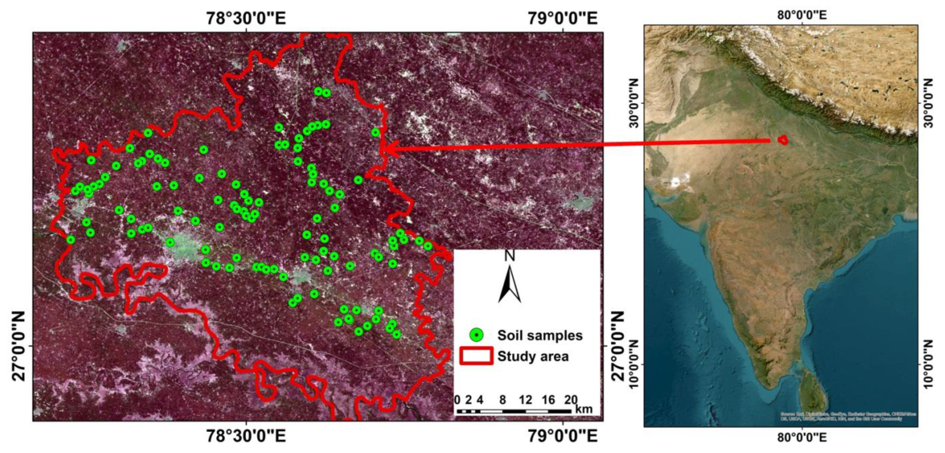
2.1. Study Area

Firozabad (situated between 26°53′ and 27°30′ N latitude, and 78°13′ E longitude) is one of the most densely populated districts of western Uttar Pradesh, India, with the majority of its population residing in rural areas (Figure 1). The Yamuna River marks the district’s western and southern boundaries, and is shared with the Agra district. The boundaries of Firozabad district touch Etah district in north and Mainpuri and Etawah districts in the east. The climate in the region is subtropical steppe experiencing ~80 rainy days with an average yearly precipitation of ~82 millimeters. The district’s topography is generally flat, with soils similar to that of the alluvial soils (Inceptisols) of the Indo-Gangetic plain (IGP) tract. With a northwest-to-south inclination, the area is primarily flat and contains four sub-divisions with nine development blocks. The district bears 821 settlements, of which 19 are abandoned. The district is mostly under cultivation for crops such as pearl millet, paddy, bajra, pigeon pea, sesame, black gram, and green gram in the kharif season, whereas wheat, mustard, barley, potato, garlic, etc., are grown in the rabi season. The soil texture varies from loam to silty clay loam, with the area being majorly affected by ravines and wasteland.

Approximately 74% of the reported total area (0.24 mha) of the district is under cultivation, with the remaining 26% of land used for purposes other than agriculture or remaining barren. The main cropping seasons in the district are Rabi, Kharif, and Zaid, with a cropping intensity of 173%, which is considerably higher than the national average. Both surface water resources and groundwater resources are used for irrigation, but later are mostly relied upon for agricultural purposes. The area inherently suffers from multi-nutrient deficiencies and a low organic carbon content, which is further aggravated by the continuous cropping of cereals and legumes in all seasons, leading to very little diversification. The region experiences extreme weather conditions, with an average annual temperature of 30.7 °C (4.76% higher than the national average). This causes organic matter to decompose faster than usual, particularly in peak summer months.

2.2. Soil Sampling and Analysis

A total of 108 soil samples were collected from a 0–15 cm depth (disturbed soil), following random soil sampling in a zig-zag manner. This study was mainly concerned with an assessment of the soil fertility, so only the surface soil depth (6 inch or 15 cm) was considered. Sampling coordinates were taken with the help of a hand-held Garmin GPS (etrex^®10). The quartering technique was adopted to reduce the sample size of the required mass. Samples were labelled and stored in plastic bags and taken to the Soil Testing Laboratory, Govind Ballabh Pant University of Agriculture and Technology, Uttarakhand, India, for processing and analysis. The soil samples were processed with a 2 mm sieve and stored in a polypropylene box. The pH of the soil–water suspension (1:2: soil: water) [29] was determined with the help of a digital pH meter (Eutech PC 700, Thermo Fisher Scientific Inc. India). The supernatant was used for analyzing the electrical conductivity (EC) using a conductivity meter (Systronics Conductivity-TDS Meter 308). The bulk density (BD) was recorded with the help of a core sampler (undisturbed soil sample) and the particle density (PD) was analyzed using a pycnometer. A keen box method was utilized to determine the water-holding capacity of the soil, while the porosity was determined using the following formula:

$$\%\mathrm{Porosity}=\left(1-\frac{\mathrm{BD}}{\mathrm{PD}}\right)\times 100$$

The potassium dichromate oxidizable organic carbon (OC) content of the soil was determined following [30]. The available nitrogen (N) in the soil samples was estimated using the alkaline KMnO₄ method [31]. The soil samples were extracted with Olsen’s reagent [32] and the phosphorus (P) content of the extract was determined using the ascorbic acid blue color method [33]. The neutral normal ammonium acetate extractable potassium (K) content [34] of the soil samples was measured using a flame photometer. Complexometric titration was used for the calcium (Ca²⁺) and magnesium (Mg²⁺) analysis [35]. The turbidimetric method was used for sulfur estimation [35] and the absorbance was measured using a spectrophotometer (Labtronics, Model LT- 291). The diethylenetriaminepentaacetic acid (DTPA)-extractable Fe, Mn, Cu, and Zn [36] were measured in the extract using atomic absorption spectroscopy (AAS) (Agilent Technologies 200 series AA).

2.3. Geostatistical Modelling

The soil fertility index (SFI) data derived from field measurements were utilized to construct spatial distribution maps using geostatistical techniques. Before the geostatistical study, the Kolmogorov–Smirnov (K–S) test for normality test was conducted. To support the assumption of a normal distribution, the data were transformed using square root transformation for the SFI. Multicollinearity and autocorrelation among the chosen variables were examined before the regression analysis. The SPSS software was used to conduct the statistical analysis.

Inverse Distance Weighing (IDW) and kriging (also known as Gaussian regression) were the two interpolation techniques used to forecast the geographical distribution of the SFI. Using Equation (1), the experimental semivariograms were created to identify the spatial dependence of the attributes.

$$\gamma \left(h\right)=1/2N\left(h\right)+{\displaystyle \sum }_{i=1}^n\left(Z\left(xi\right)+Z(xi+h\right){)}^2$$

(1)

where γ(h) is the semivariance for the interval class h, N(h) denotes the number of pairs in the lag interval, Z(xi) is the measured sample value at point i, and Z(xi + h) stands for the measured sample value at position (i + h). Simple (SK) and ordinary (OK) types were employed in order to choose the best data interpolation tool for spatial variability mapping. Using Equations (2)–(5), the most popular models of spherical, exponential, linear, and Gaussian functions were applied, respectively.

The spherical model:

$$\gamma \left(h\right)=\{\begin{array}{c}{C}_0+C\left[\frac{3h }{2a }-\frac{1}{2}{\left(\frac{h}{a}\right)}^3\right] 0\le h\le a\\ C_0+C h>a\end{array}$$

(2)

The exponential model:

$$\gamma \left(h\right)=C_0+C\left[1-exp\left(\frac{-h}{a}\right)\right]$$

(3)

The linear model:

$$\gamma \left(h\right)=C_0\left[h\left(\frac{C}{A_0}\right)\right]$$

(4)

The Gaussian model:

$$\gamma \left(h\right)=C_0+C\left[1-\exp \left(\frac{h^2}{A_0{}^2}\right)\right]$$

(5)

where C₀ is the nugget variance, C represents the structural variance, C₀ + C is the sill variance, a is the range in spatial correlation and h denotes the lag distance. The A₀ parameter of the linear model is the distance interval for the lag class and the effective range of the Gaussian model is A = 30.5A₀. According to Teegavarapu and co-workers [37], IDW uses an additive combination of values at sampled points that are weighted by an inverse function of the distance from the place of interest to the sampled points; this is in order to forecast the values of an attribute at unsampled sites. The IDW method assumes that nearby points exert greater influence on a point’s unknown value than distant points. Equation (6) was used to make predictions.

$$Z={\displaystyle \sum }_{i=1}^n\left(\raisebox{1ex}{$Z_i$}\!\left/ \!\raisebox{-1ex}{$d_i^m$}\right.\right)/{\displaystyle \sum }_{i=1}^n\left(\raisebox{1ex}{$1$}\!\left/ \!\raisebox{-1ex}{$d_i^m$}\right.\right)$$

(6)

where $Z_i$ is the measured sample value at point i, Z is the estimated value, d_i is the distance between Z and Z_i, and m is the weighting power, which indicates the ratio at which weights decrease as d_i increases. The study examined the IDW predictions using the standard 1, 2, and 3 weighting powers. Cross-validations can be used to assess the reliability of the interpolation techniques and the model’s accuracy [38,39]. In the current investigation, the best interpolation model was determined using Root Mean Square Error (RMSE). The best accurate prediction is the one with the lowest RMSE. Estimates were produced by applying the formula shown in Equation (7).

$$RMSE=\sqrt{\frac{1}{n}{\displaystyle \sum }_{i=1}^n{\left(z_i-z\right)}^2}$$

(7)

where z is the predicted value, z_i is the observed value at sampling point i (i = 1, 2…, n), and n stands for the number of sample points.

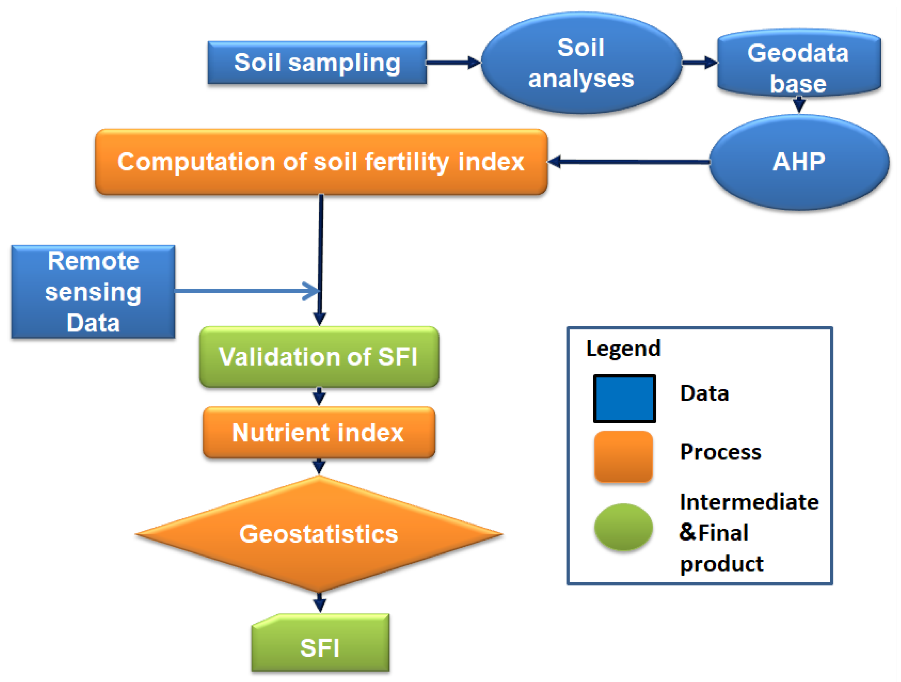
2.4. Computation of Soil Fertility Index

The soil fertility index (SFI) was computed using 17 indicators for each soil sample point as part of a parametric technique to evaluate soil fertility (Table S1). When characterizing the soil fertility, these characteristics in Table S1 are the typical inputs used for assessment. Each growth indicator for plants is rated from 10 (least favorable) to 100 (most favorable).

Equation (8) is used to determine the SFI based on each factor rating:

$$SFI=Rmax\times \left(\sqrt{\frac{A}{100}\times \frac{B}{100}\times \dots \dots \times \frac{Q}{100}}\right)$$

(8)

where R_max is the maximum ratio of (A + B +……….+ Q)/17, and A, B…, Q is the rating value of each diagnostic feature.

2.5. Validation of SFI

A methodological flowchart that illustrates an overview of the SFI computation, validation and mapping is presented in Figure 2. The various factors that affect soil fertility are numerous. Several factors, including the soil pH, EC, available N, P, and K, exchangeable Ca and Mg, and DTPA-extractable micronutrients (Fe, Mn, Zn, Cu), are generally considered when evaluating soil fertility.

To compare the soil fertility levels in one region with those in another, Ref. [40] developed the nutrient index, which assigns one value per nutrient. Three-tier (Equation (9)) and six-tier (Equation (10)) systems were proposed by the researchers, as follows:

$$Nutrient index=\frac{\left(NL\times 1+NM\times 2+NH\times 3\right) }{NT}$$

(9)

$$Nutrient index=\frac{\left(NVL\times 0.5+NL\times 1+NM\times 1.5+NMH\times 2+NH\times 2.5+NVH\times 3\right) }{NT}$$

(10)

where NT is the total number of examined samples, while NVL, NL, NM, NMH, NH, and NVH are the number of samples under very low, low, medium, moderately high, high and very high categories, respectively. The spatial variability in the various indicators employed in order to determine the SFI was captured in this instance because soil fertility varies over both time and location. The minimum soil fertility indicator (MSFI) values were converted into scored likelihood values to group similar MSFI values into classes. Figure 2 provides a summary of the processes that were undertaken in the development of the SFI. The layers of soil parameters were integrated to obtain soil fertility units for the area. The reclassification of the raster data of each physico-chemical factor was categorized into five classes. The reclassification illustrates the fertility map of each factor for land. A combination of these factor layers was incorporated into ArcMap 10.5 using the Weighted Overlay function in the Model Builder. For the weighted overlay, the level of influence (%) of each parameter was obtained using the AHP method. AHP determines the priority of each factor and takes into account the relevance of any factor to determine soil fertility. It employs a pair-wise comparison of the eigenvalue method used by AHP to assess the relative priority of each factor (Table S2). The AHP technique can convert empirical data to mathematical models. Additionally, the “consistency ratio” is computed and the values decide the effect loading on the ratings. This method of pairwise comparisons is systematic and comprehensive, and the the pairwise comparison test is often repeated if the consistency ratio values are exceptionally high. After the comparisons, the relative weights between each criterion were evaluated and the probability of each alternative was calculated (Table S3). This probability determines the likelihood that the alternative can achieve soil fertility. The higher the probability, the more likely the alternative is to satisfy the final soil fertility assessment. The priorities (or weight) of the lowest-level alternatives relative to the top objective are presented in Table S3. The weighted value obtained from AHP (% of influence) was used in the Model Builder. Finally, the overall fertility map using the factors was produced to help in locating areas of fertile soil in the region. The prioritization of the factors using AHP is displayed in

Table 1. Normalized score to prioritize the factors.

	Hydraulic Properties	Physical Properties	Chemical Properties	Pollution Properties	Slope/Land Cover/Rainfall	Row Total	% of Ratio Scale	Average	Sum	Weighted Rating	Lambda (λmax)
Hydraulic properties	0.4	0.4	0.3	0.4	0.4	2.1	0.4	0.4	2.1	2.1	5.2
Physical properties	0.2	0.2	0.3	0.2	0.2	1.1	0.2	0.2	1.1	1.2	5.2
Chemical properties	0.1	0.1	0.1	0.0	0.2	0.4	0.1	0.1	0.4	0.4	5.1
Pollution properties	0.2	0.2	0.3	0.2	0.2	1.2	0.2	0.2	1.2	1.3	5.3
Slope/Land cover/Rainfall	0.1	0.1	0.0	0.1	0.1	0.2	0.0	0.0	0.2	0.2	5.1
Column total	1.0	1.0	1.0	1.0	1.0	5.0	1.0	1.0			5.2 (Average)

and

Table 2. Prioritization of factors based on weighting.

Sl. No.	Criteria/Factors	Weight
1	Temperature	0.41
2	Rainfall	0.24
3	Altitude	0.22
4	Land cover type	0.08
5	Slope	0.05
	Total	1.00

; these results were used for weighted overlay in the GIS analysis.

To determine the soil fertility units for the region, layers of soil parameter data were amalgamated. Each physico-chemical factor’s raster data were reclassified and divided into five classes. The map of each factor for land fertility was displayed after the reclassification. These factor layers were combined and added to ArcMap 10.5 using the Model Builder’s Weighted Overlay feature. The level of effect (%) of each parameter for weighted overlay was determined using the AHP approach. The Model Builder used the weighted value (% of impact) that was obtained using AHP. Finally, a general map of fertility in the area was realized by applying the parameters. The diagram presented in Figure 2 depicts the general approach to conducting the assessment analysis using ArcGIS.

3. Results and Discussion

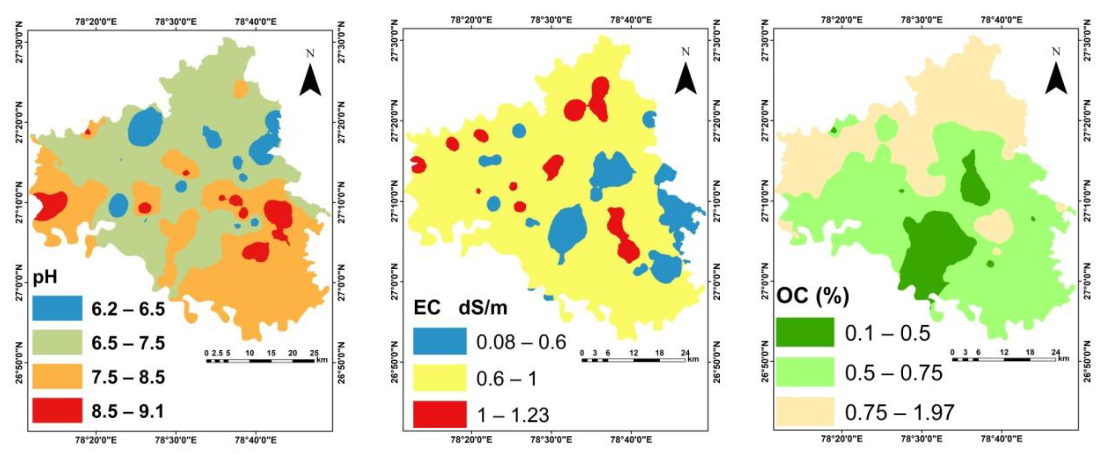
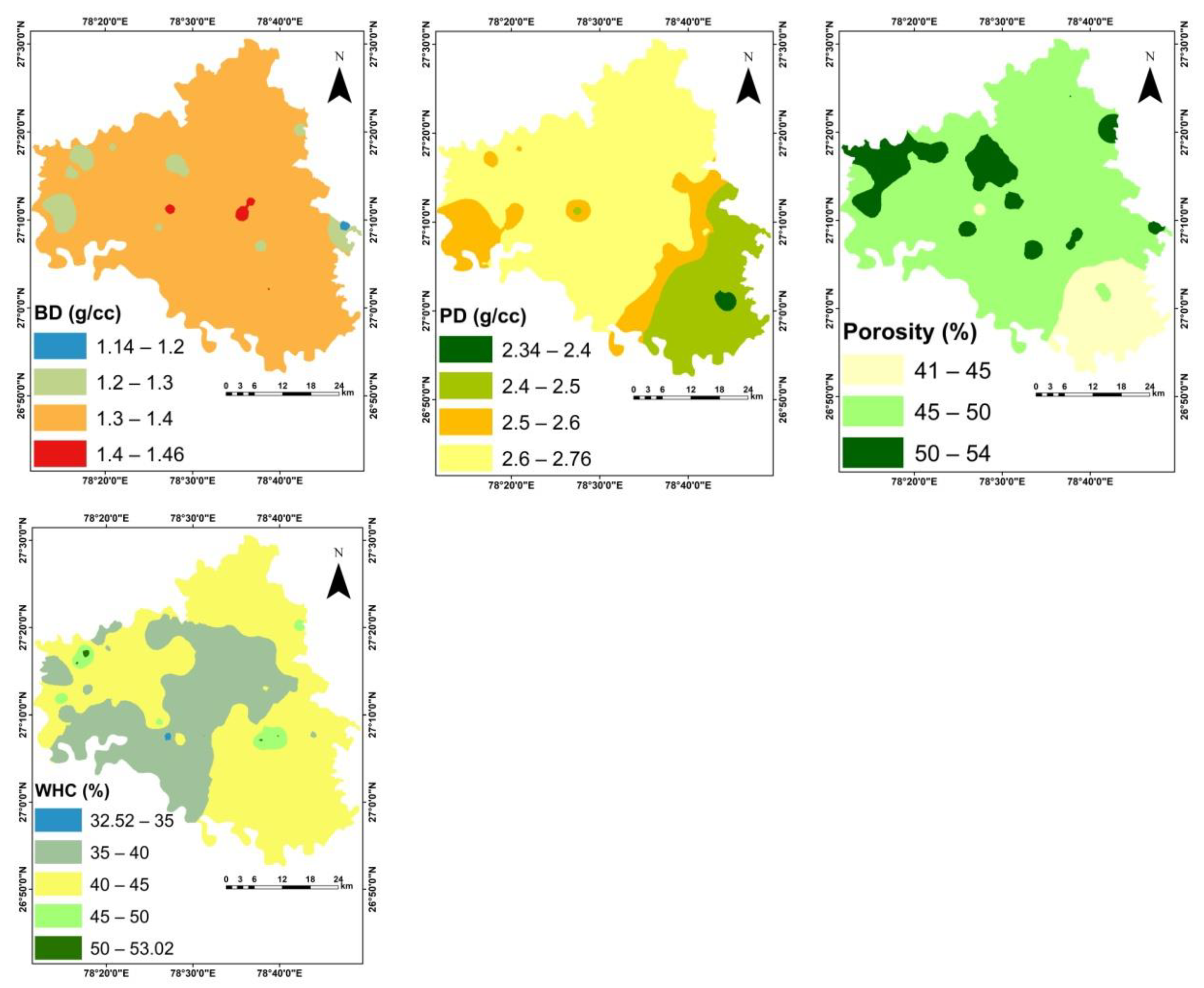
3.1. Physico-Chemical Properties of Soil

The descriptive statistics of the physical and chemical properties are presented in

Table 3. Descriptive statistics of the physico-chemical soil properties and soil fertility index.

Parameters	Min	Max	Mean	Median	SD	CV	Skewness	Kurtosis
pH	6.2	9.1	7.61	7.5	0.55	7.26	0.5	0.22
EC (dS m−1)	0.08	1.23	0.41	0.35	0.26	61.7	1	0.39
BD (g cc−1)	1.14	1.46	1.34	1.34	0.05	3.81	−0.41	1.37
PD (g cc−1)	2.34	2.76	2.6	2.63	0.1	3.93	−0.96	−0.04
Porosity (%)	40.7	54.0	48.5	49.2	2.74	5.64	−1.1	0.9
WHC (%)	32.5	53.0	40.5	40.3	4.34	10.7	0.69	0.38
SOC (%)	0.1	1.97	0.71	0.65	0.33	46.5	1.49	2.98
N (kg ha−1)	150.2	490.3	263.0	267.7	59.3	22.6	0.63	1.52
P (kg ha−1)	10.1	37.1	24.3	24.7	7.1	29.3	−0.21	−1.01
K (kg ha−1)	121.7	504	285.0	284.3	80.1	28.1	0.27	−0.32
Ca (cmol(p+) kg−1)	0.8	40.2	13.0	12.4	7.88	60.5	0.77	1.12
Mg (cmol(p+) kg−1)	1.2	91.1	30.8	25.9	24.5	79.6	1.01	0.13
S (mg kg−1)	0.97	22.2	5.56	4.8	3.62	65.2	1.81	5.12
Fe (mg kg−1)	1.2	20.9	4.74	3.22	3.77	79.6	2.14	4.24
Mn (mg kg−1)	0.14	12.3	2.66	0.55	3.84	144.3	1.31	0.05
Cu (mg kg−1)	0.6	4.88	2.86	3.72	1.42	49.5	−0.36	−1.64
Zn (mg kg−1)	0.21	3.0	0.63	0.31	0.62	99.4	1.87	2.91

.

The results of this study show variation, which is attributed to the dynamic interactions between the natural environmental elements, such as the degree of soil development, and methods of land use and management. The study area was within the agro-climatic zone of the south-western semi-arid region and had a soil pH in the range of 6.2–9.1, which is mainly categorized as slightly acidic to strongly alkaline [41]. The Firozabad district is part of the Indo-Gangetic plain, whose soils are mostly alluvial in nature. The soils were non-saline (<2 dS m⁻¹) with electrical conductivity (EC) values ranging between 0.08 and 1.23 dS m⁻¹. Such variation in the EC values, which lay within <2 dS m⁻¹, indicated that most of the plants, except for a few legumes (such as cowpea and bean), vegetable crops, including potato, onion, okra, eggplant, etc., and some field crops, could be easily grown in these soils without much of an adverse effect on the yield due to the existing EC values of soil [42]. The salt tolerance of crops could be judged by the salinity threshold (EC_t) and the % reduction in yield with every unit increase in EC above the threshold limit. The above-mentioned plants have EC_t values of <2 dS m⁻¹, thus placing restrictions on the growth of these crops [43].

The bulk density (BD) and particle density (PD) varied between 1.14–1.46 g cc⁻¹ and 2.34–2.76 g cc⁻¹, respectively, with an average value of 1.34 and 2.6 g cc⁻¹, respectively. The average Walkley–Black soil organic content was 0.71% (0.1–1.97%). By and large, the soil samples were low in organic carbon, which could be attributed to the high temperature in the region leading to the faster oxidation of organic matter [44,45]. Most of the area (56.5% of the soil samples) was found to be low in available N content, and the rest had medium levels of available N (43.5% samples). The average N content in the soil was 263.0 kg ha⁻¹ (150.2 to 490.3 kg ha⁻¹). This is quite natural considering the minimal organic matter content in the soil. Organic matter is deemed to be the most critical indicator of soil fertility and they are considered to have a direct relationship [46]. The concentration of OC in the study area was low, thus affecting the various nutrient cycling processes and causing low N availability in the soil. As high as 62% of the soil samples were sufficient in available P, while 35.2% of the samples had medium levels of available P. On average, the study area was sufficient in available P, exhibiting values higher than 22 kg P ha⁻¹. In total, 50% of the soil samples were sufficient in available K content, while the rest had medium concentrations of available K content. The study region is a part of the IGP tract and the soils share their origin with alluvium sediments. Alluvial soils present in the IGP tract have a large amount of mica/illite clay minerals in clay and silt fractions, thus providing a very large reserve of K to the soil [47,48]. As far as the DTPA-extractable micronutrients content in soil is concerned, all the soils were found to be sufficient in Cu (2.86 mg kg⁻¹ (average); 0.6–4.88 mg kg⁻¹ (range)), while approximately 75% of the samples were deficient in Fe (4.74 mg kg⁻¹; 1.20–20.9 mg kg⁻¹), Mn (2.66 mg kg⁻¹; 0.14–12.3 mg kg⁻¹), and Zn (0.63 mg kg⁻¹; 0.21–3.00 mg kg⁻¹) content.

The CV is the most important measure for defining the variability in soil parameters [49]. A CV value of ≤20% is categorized under the low variability class, a value of 21% < CV ≤ 50% is categorized as moderate variability, a value of 51% < CV ≤ 100% is categorized as high variability, and CV > 100% indicates very high variability [50]. The CV values presented in Table 3 reveal a low variability in the distribution of pH and all the physical properties of soil, such as BD, PD, porosity %, and WHC. The distribution of SOC and available N, P, K, and DTPA-extracted Cu is moderately variable, while the distribution of EC, Ca, Mg, S, Fe, Zn, and Cu is more highly variable in the study area. Unusually, very high variability was observed in the distribution of DTPA-extracted Mn in the study area.

The above results confirm that the interference of humans through agricultural activities and the very heavy usage of fertilization leads to greater variability in the distribution of various chemicals in the soil or in soil fertility parameters, including SOC. The high variation in plants’ essential nutrients in the area could be attributed to land usage and the build-up of biomass from litterfall and root biomass [51]. However, the minimal variability in the soil’s physical properties reveals the strong role played by soil texture in diminishing the effect of continuous cultivation on these properties. Most of the essential plant nutrients, except P and Cu, were positively skewed which indicated that fertilization, crop residue decomposition and nutrient cycling processes have a strong effect on nutrient concentrations. This was further substantiated by the fact that these nutrients (except P and Cu) had greater mean values than their respective median values (Table 3).

3.2. The Semivariograms of Soil Fertility Indicators

The parameters of semivariograms were calculated and the best-fitted model among the Gaussian, linear, spherical, and exponential models was selected based on RMSE values (

Table 4. RMSE values of cross-validations according to interpolation models.

Criteria	Inverse Distance Weighing-IDW
	IDW-1		IDW-2		IDW-3		IDW-4
SFI	0.5397		0.5397		0.5453		0.5546
	Ordinary Kriging				Simple Kriging
	Gaussian	Exponential	Spherical	Linear	Gaussian	Exponential	Spherical	Linear
SFI	0.5291	0.5454	0.5523	0.5552	0.5323	0.5201	0.5333	0.5260

).

The chemical properties of the soil had a nugget-to-sill (C₀/(C + C₀)) ratio of less than 25%, which indicates their high spatial association [46]. The range in the parameters was the distance in which the samples could affect each other. Such a distance indicates the correlation among the samples and the minimum distance that is essential for sampling. The results indicated that IDW was the most suitable method for the prediction of soil properties with minimum RMSE values. The cross-validation method (using Root Mean Square Error (RMSE)) indicated that the interpolation methods were able to predict the spatial variability in the measured parameters; however, simple kriging (SK) was the best one for predicting soil spatial variability for the more efficient management of agricultural lands utilizing different practices (Table 4). Although the topography is generally flat, with elevation ranging from less than 1000 feet above sea level to as high as 2000 feet, generally, the area is marked by rolling hills. The chemical properties of the soil were significantly affected by different land use types, such as cultivated and bare soils. Salinity was the highest in the lowlands and the lowest in the upper areas. The highest and the smallest values of N and SOC resulted from uncultivated land.

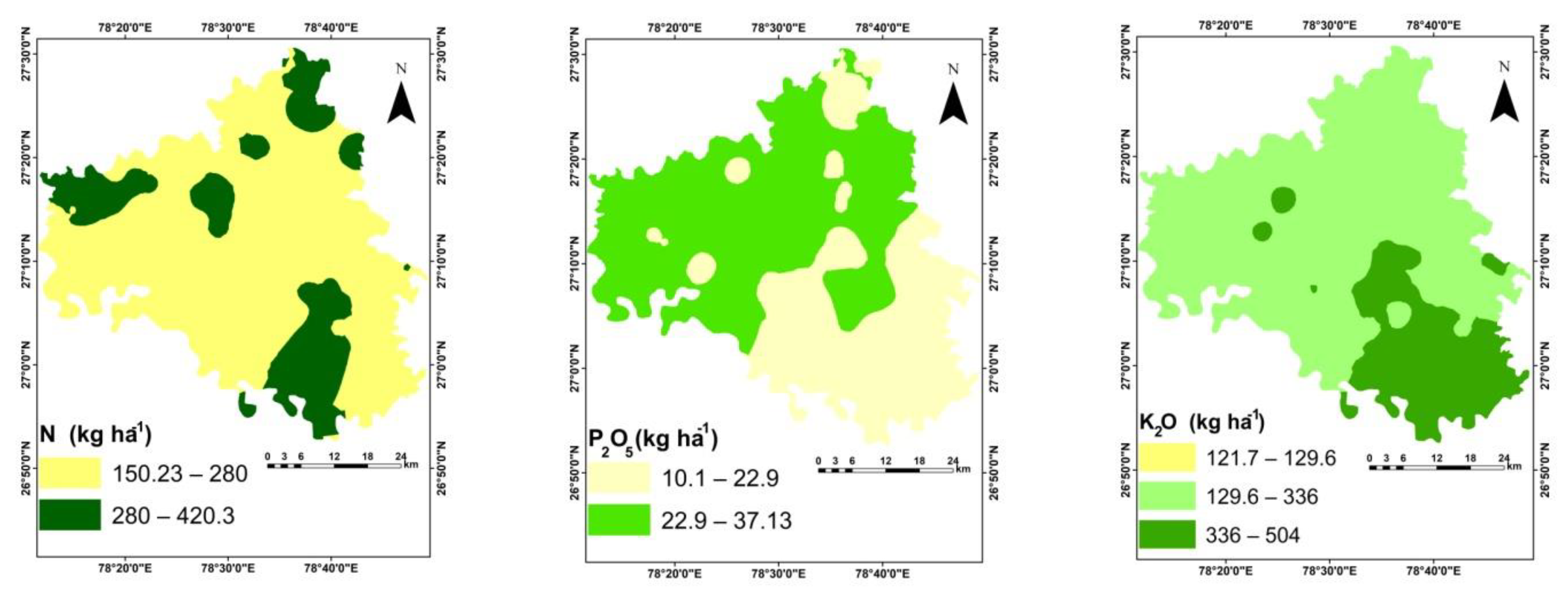
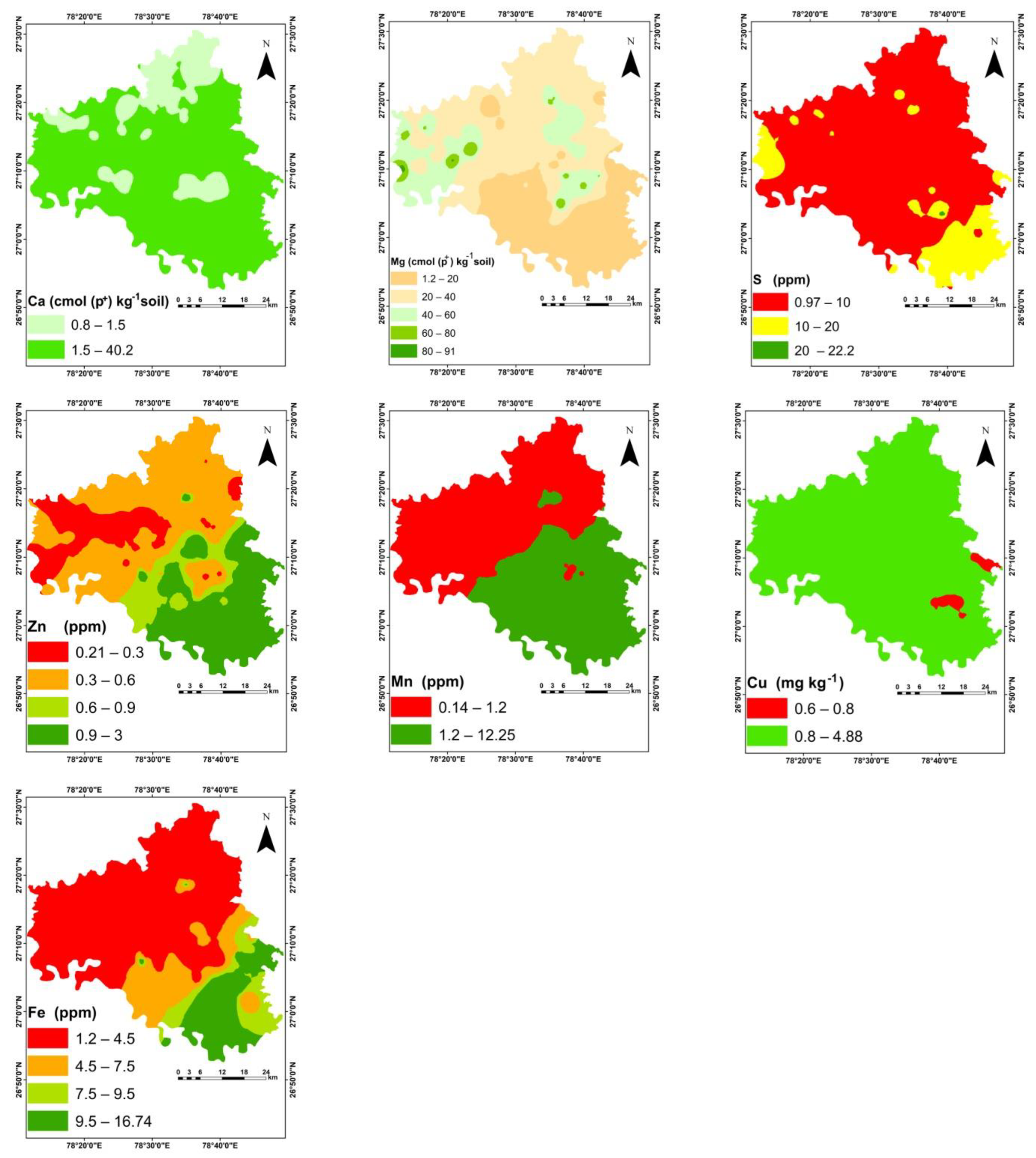
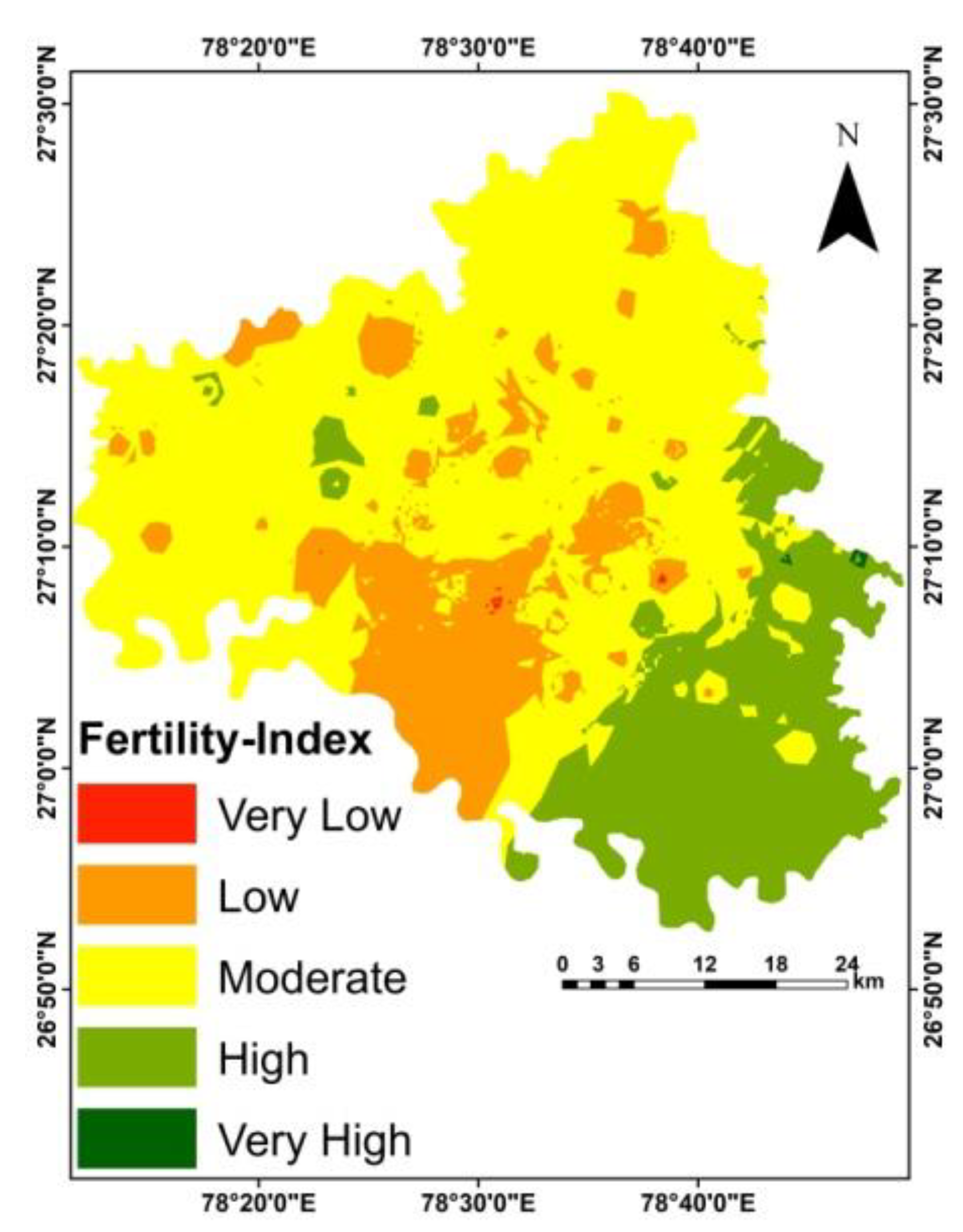
3.3. Spatial Distribution of Soil Fertility Indicators and SFI

In the present research, the spatial variability in the soil parameters with different types of land use and at different altitudes was determined. There was high variation among the measured parameters, and the sources of variation, including the land use type and altitude, significantly affected the statistical and geostatistical variability in the observed and predicted variables. It is crucial to comprehend the spatial variability using the convenient geostatistical semivariogram model to map and define the diverse area ranges and to employ the best management tactics [52]. The SFI estimate in the study area was compared by using the IDW and kriging interpolation techniques. Before performing the geostatistical interpolation, semivariogram models in four directions were made to detect the anisotropy. The anisotropy in the semivariograms did not considerably vary from one to another. A comparison of the SFI interpolation methods is shown in Table 4. Tests were run on the four variograms of OK (spherical, exponential, Gaussian, and linear), SK (spherical, exponential, Gaussian, and linear), and IDW to determine the best results. Despite having identical power, IDW-1 and IDW-2 demonstrated higher RMSE values. The lowest RMSE values were provided by the OK and SK methods. The data of the RMSE values presented in Table 4 reveal that the exponential variogram of SK performed as the best-fit model for SFI.

Innumerable factors can affect the chemical properties of a region’s soil over space and time. Human-created factors, such as crop management practices, the selection of crops/cropping sequences, nutrient management practices, etc., take a significant toll on natural factors [53,54]. The present state of soil fertility is mostly governed by the extent of regulated/unregulated farm operations. It has been observed that the areas that are significantly affected by human activities (farming) have poor spatial dependence on the chemical properties of soil [12]. However, in our study, the different chemical properties of soil indicated very high levels of spatial dependence, as deduced from the sill-to-nugget ratio of <25%. The spatial variability maps of different physical and chemical properties of the Firozabad district are presented in Figure 3.

An examination of the maps reveals that the physical properties, such as DB, PD, WHC, and % porosity, have very little spatial variation throughout the region. The average elevation of the study region is around 150 m above mean sea level (MSL), which can be categorized under plain land. Topography affects various physical properties of the soil, such as soil texture, structure, soil bulk density, thermal properties, etc. [55]. The region displays very minimal variation in elevation, which indicates the negligible effect of topography on the physical properties of soil. Ofori and co-workers [56] reported that the distribution of coarser soil particles, such as sand, was mostly detected in the upper slopes, while the finer particles were higher in proportion towards the downhill region. The processes occurring in surface soils, such as the erosion rate, depth-wise distribution of water, and microbial activity, were found to be critically affected by topography [12]. Consequently, it is essential to interpret the influence of topography on the physical properties of soil in a region to understand the spatial variability of these properties. In our study, the low spatial variability of the assessed soil physical parameters could be attributed to the minimal difference between the maximum and minimum elevation, as well as the planar surface of the region.

Soil pH is considered to have a strong effect on plant nutrient availability, therefore, unarguably, it has been named the master variable that governs the soil’s chemical and biochemical functions [57]. The soils of the study region suggest the transition from slightly acidic to strongly alkaline pH conditions, indicating the crucial role played by some external factors that have overcome the buffering mechanism of soil and have elevated the pH to levels sufficiently critical to affect plant growth. The higher pH in cultivated lands is due to fertilization and cultivation, which can affect carbon cycling. Significant differences were evident among different land use types and their effects on the properties of the soil. There are differences between the rangeland and the uncultivated land, which could be due to insufficient drainage. A spatiotemporal variability study of soil fertility indicators was carried out by Chen et al. [46] over a decade. Their study found that after continuous cropping in Jianli County, China, the soil pH increased to a more alkaline range due to the continuous application of fertilizer salts and alkaline irrigation water. The CV of soil pH values was quite low (Table 3) in the soil samples from the study region. Such results corroborate the findings of other published research, which has shown CV values of <10% in the case of soil pH [46,58,59].

It is quite interesting to note such low spatial variability in the soil pH at the district level, which confirms the strong buffering mechanisms in action in the study area by various cationic and anionic compounds present in the soil. The spatial variability map of EC presented in Figure 3 shows that the regions with higher pH levels correspondingly revealed higher EC values of 0.6–1 dS m⁻¹ and 1–1.23 dS m⁻¹. The high EC values could be attributed to the application of fertilizer salts, and organic manures to the soil during crop production over the years [60].

Different land use types in the study area have significantly affected the various chemical properties, such as SOC content and essential plant macro and micronutrient availability, to a greater extent. Almost the entire mainland can be classified as agricultural lands with sparse settlements, uncultivated lands, forest areas, and plantation fields extending towards the southern parts. The region’s cropping intensity well exceeds the national average. Among the nine blocks in the entire district, Madanpur and Shikohabad have considerably higher cropping intensities, of 205% and 198%, respectively. This explains the higher availability of essential macronutrients, including N, P and K, for these blocks in the southern parts of the district, as illustrated in Figure 4.

The N availability in the region is found to vary within the medium range of 280–560 kg ha⁻¹. A comparison of the descriptive statistics results presented in Table 4 indicates that N varies from 150.2–490.3 kg ha⁻¹, thus generating moderate variability in the region. This was quite natural considering a somewhat similar cropping intensity throughout the region, thus indicating similar residue additions over the year. The majority of the area grows wheat, which is followed by vegetable crops. Revealed here is that more or less similar fertilizer application rates are being followed in the study area, thus giving less scope for NPK variability in the region. The uniform agronomic practices followed throughout the region reduce the variability in essential plant nutrients in the soil and play a major role in homogenizing the data sets [61]. Although, indeed, the selection of the source and the mode of applying fertilizer products varies among farmers in the region, the fact remains that farmers without exception apply NPK to the soil, and this cannot be overlooked. In the case of micronutrients, the spatial variability in their distribution was quite high (Table 3; Figure 4). This could be attributed to the non-uniform adoption of balanced fertilizer application practices by farmers and, based on the socio-economic circumstances of farmers in the region, the selective application of nutrient elements to soil.

The distribution map of the SFI is broken down into five levels in the study area, as depicted in Figure 5 below.

Because human-induced disturbances and the characteristics of natural ecosystems have an impact on soil quality, soils have heterogeneous features (e.g., fertilization and irrigation) [62]. As a result, the interplay between natural and agricultural management elements has led to the spatial SFI pattern of the farmed land. Very high (F1) and high (F2) fertility was present in around 16% of the study region (

Table 5. List of the classes of the soil fertility index and their distribution.

Class	Definition	SFI Index Value	Area (ha)	Area (%)
F1	Very highly fertile	>8.953	136.58	0.05
F2	Highly fertile	7.695–8.953	41,274.54	16.59
F3	Moderately fertile	6.208–7.695	151,616.08	60.94
N1	Low fertile	4.455–6.208	55,581.93	22.34
N2	Very low fertile	<4.455	168.76	0.07
Total			248,777.89	100.0

), primarily in the south and eastern parts of the Firozabad district (Figure 5).

A major part of the north-central and western regions of the district showed moderate fertility (~61%). These areas are suitable for agricultural activities, especially when animal or green manure is additionally applied in order to trigger aggregation, develop the soil structure and increase the activity of microorganisms in the soil [62,63]. About 22.4% of the study area that was classified as having low and very low fertility was located in the northern part, due to a strong alkali reaction (pH value > 8.0), a low OC content, and low plant nutrient availability. These locations are suitable for farming, particularly when advice is followed regarding the additional application of animal or green manure so as to encourage aggregation, the formation of soil structure, and improved soil microbial activity under appropriate tillage techniques. This suggests that the management of soils at the sub-field level can help improve crop yield and quality [63,64]. Overall, this study provided some useful information about the physico-chemical and nutrient properties of the soil samples collected from the study area. Several factors influence the physical, chemical, and biological characteristics of soil, including the climate, topography, land use, and management practices. The physical properties of soil can be used as a key indicator for soil management, as they can also define the type of soil and the long-term management practices required for successful crop production.

4. Conclusions

In the field of soil fertility management, the ability of policymakers and the public to determine soil fertility is very important, so that they can better understand the status of soil health. This study found that the soils of the Firozabad district were low in organic carbon and available N content, while other macronutrients, such as P and K, were found in sufficient levels in the soils. In the case of micronutrients, our study shows that the soil was deficient in all (except Cu) micronutrients, including Fe, Mn, and Zn. Overall, the Firozabad district was found to have a medium level of soil fertility. The computation of the SFI infers that the south and southeastern region of the study area had very high levels of soil fertility. The spatial distribution of the SFI was impacted by its coefficients of variation, which varied as a result of the soil being formed by alluvial parent materials, as recorded using the interpolation techniques.

The map presented in this study will provide an overview of soil quality for non-academics and end users so that they can gauge the soil’s fertility. However, insights and lessons learned from this study may be applied universally, even if they are limited to the study area. Many developing countries, including other parts of India, share the same soil fertility issues as the current study area. Due to climate change, and alterations in rainfall frequency, soil quality and fertility could result from a combination of arid/semi-arid climate, geological risks, and anthropogenic activities in those regions. To monitor these soil resources for proper decision-making, the use of GIS platforms and soft computing techniques offers the chance to create more accurate soil fertility/quality maps.

We recommend and encourage future researchers to use the SFI map as the foundation for defining the various management zones in which soil deterioration must be combated so that viable and sustainable agriculture can continue into the future, as based on the findings of this study. Finally, this paper demonstrates the potential of merging remote sensing vegetation-related indices to validate an advanced fertility model that is appropriate for regions with semi-arid climates.

References

1. FAO. Status of the World’s Soil Resources (SWSR)—Main Report; Food and Agriculture Organization of the United Nations and Intergovernmental Technical Panel on Soils: Rome, Italy, 2015; p. 650. [Google Scholar]
2. Majhi, P.K.; Raza, B.; Behera, P.P.; Singh, S.K.; Shiv, A.; Mogali, S.C.; Bhoi, T.K.; Patra, B.; Behera, B. Future-Proofing Plants Against Climate Change: A Path to Ensure Sustainable Food Systems. In Biodiversity, Functional Ecosystems and Sustainable Food Production; Springer: Berlin/Heidelberg, Germany, 2022; pp. 73–116. [Google Scholar]
3. Verma, R.K.; Singh, A.; Hasanain, M.; Raza, M.B.; Singh, R.K. Nitrogen Management Practices for Improving Yield and Nitrogen Use Efficiency in Rice (Oryza Sativa). Indian J. Agric. Sci. 2020, 90, 1342–1344. [Google Scholar] [CrossRef]
4. Megahed, H.A. GIS-Based Assessment of Groundwater Quality and Suitability for Drinking and Irrigation Purposes in the Outlet and Central Parts of Wadi El-Assiuti, Assiut Governorate, Egypt. Bull. Natl. Res. Cent. 2020, 44, 187. [Google Scholar] [CrossRef]
5. Sharma, S.; Singh, Y.V.; Saraswat, A.; Prajapat, V.; Kashiwar, S.R. Groundwater Quality Assessment of Different Villages of Sanganer Block in Jaipur District of Rajasthan. J. Soil Salin. Water Qual. 2021, 13, 248–254. [Google Scholar]
6. Mujiyo, M.; Suntoro, S.; Akbar, R.R.; Rahayu, R. Mapping of Agricultural Land Use Change and Effect on Land Capability as a Basis for Land Use Direction in Nguntoronadi-Indonesia. Int. J. Agric. Syst. 2022, 10, 13–25. [Google Scholar] [CrossRef]
7. De Feudis, M.; Falsone, G.; Gherardi, M.; Speranza, M.; Vianello, G.; Antisari, L.V. GIS-Based Soil Maps as Tools to Evaluate Land Capability and Suitability in a Coastal Reclaimed Area (Ravenna, Northern Italy). Int. Soil Water Conserv. Res. 2021, 9, 167–179. [Google Scholar] [CrossRef]
8. Priori, S.; Pellegrini, S.; Vignozzi, N.; Costantini, E.A.C. Soil Physical-Hydrological Degradation in the Root-Zone of Tree Crops: Problems and Solutions. Agronomy 2020, 11, 68. [Google Scholar] [CrossRef]
9. AbdelRahman, M.A.E.; Metwaly, M.M.; Afifi, A.A.; D’Antonio, P.; Scopa, A. Assessment of Soil Fertility Status under Soil Degradation Rate Using Geomatics in West Nile Delta. Land 2022, 11, 1256. [Google Scholar] [CrossRef]
10. AbdelRahman, M.A.E.; Saleh, A.M.; Arafat, S.M. Assessment of Land Suitability Using a Soil-Indicator-Based Approach in a Geomatics Environment. Sci. Rep. 2022, 12, 18113. [Google Scholar] [CrossRef]
11. AbdelRahman, M.A.E.; Engel, B.; SM Eid, M.; Aboelsoud, M.H. A New Index to Assess Soil Sustainability Based on Temporal Changes of Soil Measurements Using Geomatics–An Example from El-Sharkia, Egypt. All Earth 2022, 34, 147–166. [Google Scholar] [CrossRef]
12. AbdelRahman, M.A.E.; Natarajan, A.; Hegde, R. Assessment of Land Suitability and Capability by Integrating Remote Sensing and GIS for Agriculture in Chamarajanagar District, Karnataka, India. Egypt. J. Remote Sens. Space Sci. 2016, 19, 125–141. [Google Scholar] [CrossRef] [Green Version]
13. Tiwari, K.R.; Sitaula, B.K.; Borresen, T.; Bajracharya, R.M. An Assessment of Soil Quality in Pokhare Khola Watershed of the Middle Mountains in Nepal. J. Food Agric. Environ. 2006, 4, 276. [Google Scholar]
14. Hombegowda, H.C.; Adhikary, P.P.; Jakhar, P.; Madhu, M. Alley Cropping Agroforestry System for Improvement of Soil Health. In Soil Health and Environmental Sustainability: Application of Geospatial Technology; Springer: Berlin/Heidelberg, Germany, 2022; pp. 529–549. [Google Scholar]
15. Guo, L.; Sun, Z.; Ouyang, Z.; Han, D.; Li, F. A Comparison of Soil Quality Evaluation Methods for Fluvisol along the Lower Yellow River. Catena 2017, 152, 135–143. [Google Scholar] [CrossRef]
16. Armenise, E.; Redmile-Gordon, M.A.; Stellacci, A.M.; Ciccarese, A.; Rubino, P. Developing a Soil Quality Index to Compare Soil Fitness for Agricultural Use under Different Managements in the Mediterranean Environment. Soil Tillage Res. 2013, 130, 91–98. [Google Scholar] [CrossRef]
17. Amorim, H.C.S.; Ashworth, A.J.; Brye, K.R.; Wienhold, B.J.; Savin, M.C.; Owens, P.R.; Silva, S.H.G. Soil Quality Indices as Affected by Long-term Burning, Irrigation, Tillage, and Fertility Management. Soil Sci. Soc. Am. J. 2021, 85, 379–395. [Google Scholar] [CrossRef]
18. Amorim, H.C.S.; Ashworth, A.J.; Wienhold, B.J.; Savin, M.C.; Allen, F.L.; Saxton, A.M.; Owens, P.R.; Curi, N. Soil Quality Indices Based on Long-term Conservation Cropping Systems Management. Agrosyst. Geosci. Environ. 2020, 3, e20036. [Google Scholar] [CrossRef] [Green Version]
19. Manivannan, S.; Khola, O.P.S.; Kannan, K.; Hombegowda, H.C.; Singh, D.V.; Sundarambal, P.; Thilagam, V.K. Comprehensive Impact Assessment of Watershed Development Projects in Lower Bhavani Catchments of Tamil Nadu. J. Soil Water Conserv. 2021, 20, 66–73. [Google Scholar] [CrossRef]
20. Oladipo, J.O.; Aboyeji, O.S.; Akinwumiju, A.S.; Adelodun, A.A. Fuzzy Logic Interference for Characterization of Surface Water Potability in Ikare Rural Community, Nigeria. J. Geovis. Spat. Anal. 2020, 4, 1. [Google Scholar] [CrossRef]
21. Mora-Herrera, D.Y.; Guillaume, S.; Snoeck, D.; Escobar, O.Z. A Fuzzy Logic Based Soil Chemical Quality Index for Cacao. Comput. Electron. Agric. 2020, 177, 105624. [Google Scholar] [CrossRef]
22. Ogunleye, G.O.; Fashoto, S.G.; Mashwama, P.; Arekete, S.A.; Olaniyan, O.M.; Omodunbi, B.A. Fuzzy Logic Tool to Forecast Soil Fertility in Nigeria. Sci. World J. 2018, 2018, 3170816. [Google Scholar] [CrossRef]
23. Prabakaran, G.; Vaithiyanathan, D.; Ganesan, M. Fuzzy Decision Support System for Improving the Crop Productivity and Efficient Use of Fertilizers. Comput. Electron. Agric. 2018, 150, 88–97. [Google Scholar] [CrossRef]
24. Prabakaran, G.; Vaithiyanathan, D.; Ganesan, M. Soil Fertility Review using Fuzzy Logic. J. Eng. Res. 2021, 192, 202. [Google Scholar] [CrossRef]
25. Aliyu, K.T.; Kamara, A.Y.; Jibrin, J.M.; Huising, J.E.; Shehu, B.M.; Adewopo, J.B.; Mohammed, I.B.; Solomon, R.; Adam, A.M.; Samndi, A.M. Delineation of Soil Fertility Management Zones for Site-Specific Nutrient Management in the Maize Belt Region of Nigeria. Sustainability 2020, 12, 9010. [Google Scholar] [CrossRef]
26. El Behairy, R.A.; El Baroudy, A.A.; Ibrahim, M.M.; Mohamed, E.S.; Kucher, D.E.; Shokr, M.S. Assessment of Soil Capability and Crop Suitability Using Integrated Multivariate and GIS Approaches toward Agricultural Sustainability. Land 2022, 11, 1027. [Google Scholar] [CrossRef]
27. Metwally, M.S.; Shaddad, S.M.; Liu, M.; Yao, R.-J.; Abdo, A.I.; Li, P.; Jiao, J.; Chen, X. Soil Properties Spatial Variability and Delineation of Site-Specific Management Zones Based on Soil Fertility Using Fuzzy Clustering in a Hilly Field in Jianyang, Sichuan, China. Sustainability 2019, 11, 7084. [Google Scholar] [CrossRef] [Green Version]
28. Saaty, T.L. The Analytical Hierarchy Process: Planning, Priority Setting, Resource Allocation; McGraw-Hill: New York, NY, USA, 1980. [Google Scholar]
29. Datta, S.P.; Rao, A.S.; Ganeshamurthy, A.N. Effect of Electrolytes Coupled with Variable Stirring on Soil PH. J. Indian Soc. Soil Sci. 1997, 45, 185–187. [Google Scholar]
30. Walkley, A.; Black, I.A. An Examination of the Degtjareff Method for Determining Soil Organic Matter, and a Proposed Modification of the Chromic Acid Titration Method. Soil Sci. 1934, 37, 29–38. [Google Scholar] [CrossRef]
31. Subbiah, B.V.; Asija, G.L. A Rapid Method for the Estimation of Nitrogen in Soil. Curr. Sci. 1956, 26, 259–260. [Google Scholar]
32. Olsen, S.R. Estimation of Available Phosphorus in Soils by Extraction with Sodium Bicarbonate; US Department of Agriculture: Washington, DC, USA, 1954.
33. Watanabe, F.S.; Olsen, S.R. Test of an Ascorbic Acid Method for Determining Phosphorus in Water and NaHCO3 Extracts from Soil. Soil Sci. Soc. Am. J. 1965, 29, 677–678. [Google Scholar] [CrossRef]
34. Jackson, M.L. Soil Chemical Analysis: Advanced Course; UW-Madison Libraries Parallel Press: Madison, WI, USA, 2005. [Google Scholar]
35. Singh, D.; Chhonkar, P.K.; Dwivedi, B.S. Manual on Soil, Plant and Water Analysis; Westville Publishing House: Delhi, India, 2005. [Google Scholar]
36. Lindsay, W.L.; Norvell, W. Development of a DTPA Soil Test for Zinc, Iron, Manganese, and Copper. Soil Sci. Soc. Am. J. 1978, 42, 421–428. [Google Scholar] [CrossRef]
37. Teegavarapu, R.S.V.; Chandramouli, V. Improved Weighting Methods, Deterministic and Stochastic Data-Driven Models for Estimation of Missing Precipitation Records. J. Hydrol. 2005, 312, 191–206. [Google Scholar] [CrossRef]
38. Isaaks, E.H.; Srivastava, R.M. Applied Geostatistics; Oxford University Press: New York, NY, USA, 1989; Volume 561. [Google Scholar]
39. Eldeiry, A.A.; Garcia, L.A. Comparison of Ordinary Kriging, Regression Kriging, and Cokriging Techniques to Estimate Soil Salinity Using LANDSAT Images. J. Irrig. Drain. Eng. 2010, 136, 355–364. [Google Scholar] [CrossRef]
40. Parker, F.W.; Nelson, W.L.; Winters, E.; Miles, I.E. The Broad Interpretation and Application of Soil Test Information. Agron. J. 1951, 43, 105–112. [Google Scholar] [CrossRef]
41. Kellogg, C.E. Soil Survey Division Staff: Soil Survey Manual; United States Department of Agriculture: Washington, DC, USA, 1993.
42. Machado, R.M.A.; Serralheiro, R.P. Soil Salinity: Effect on Vegetable Crop Growth. Management Practices to Prevent and Mitigate Soil Salinization. Horticulturae 2017, 3, 30. [Google Scholar] [CrossRef] [Green Version]
43. Snapp, S.S.; Shennan, C.; Van Bruggen, A.H.C. Effects of Salinity on Severity of Infection by Phytophthora Parasitica Dast., Ion Concentrations and Growth of Tomato, Lycopersicon Esculentum Mill. New Phytol. 1991, 119, 275–284. [Google Scholar] [CrossRef]
44. Kirschbaum, M.U.F. The Temperature Dependence of Organic-Matter Decomposition—Still a Topic of Debate. Soil Biol. Biochem. 2006, 38, 2510–2518. [Google Scholar] [CrossRef]
45. Pawar, A.B.; Kumawat, C.; Verma, A.K.; Meena, R.K.; BasitRaza, M.; Anil, A.S.; Trivedi, V.K. Threshold Limits of Soil in Relation to Various Soil Functions and Crop Productivity. Int. J. Curr. Microbiol. Appl. Sci. 2017, 6, 2293–2302. [Google Scholar] [CrossRef] [Green Version]
46. Chen, S.; Lin, B.; Li, Y.; Zhou, S. Spatial and Temporal Changes of Soil Properties and Soil Fertility Evaluation in a Large Grain-Production Area of Subtropical Plain, China. Geoderma 2020, 357, 113937. [Google Scholar] [CrossRef]
47. Sahoo, J.; Dinesh, B.M.A.; Anil, A.S.; Raza, M. Nutrient Distribution and Relationship with Soil Properties in Different Watersheds of Haryana. Indian J. Agric. Sci. 2020, 90, 172–177. [Google Scholar] [CrossRef]
48. Das, D.; Sahoo, J.; Raza, M.B.; Barman, M.; Das, R. Ongoing Soil Potassium Depletion under Intensive Cropping in India and Probable Mitigation Strategies. A Review. Agron. Sustain. Dev. 2022, 42, 4. [Google Scholar] [CrossRef]
49. Saraswat, A.; Nath, T.; Omeka, M.; Unigwe, C.O.; Anyanwu, I.E.; Ugar, S.I.; Latare, A.; Raza, M.B.; Behera, B.; Adhikary, P.P. Irrigation Suitability and Health Risk Assessment of Groundwater Resources in the Firozabad Industrial Area of North-Central India: An Integrated Indexical, Statistical, and Geospatial Approach. Front. Environ. Sci. 2023, 11, 296. [Google Scholar] [CrossRef]
50. Du, H.; Lu, X. Spatial Distribution and Source Apportionment of Heavy Metal (Loid) s in Urban Topsoil in Mianyang, Southwest China. Sci. Rep. 2022, 12, 10407. [Google Scholar] [CrossRef]
51. Behera, B.; Das, T.K.; Raj, R.; Ghosh, S.; Raza, M.B.; Sen, S. Microbial Consortia for Sustaining Productivity of Non-Legume Crops: Prospects and Challenges. Agric. Res. 2021, 10, 1–14. [Google Scholar] [CrossRef]
52. AbdelRahman, M.A.E.; Zakarya, Y.M.; Metwaly, M.M.; Koubouris, G. Deciphering Soil Spatial Variability through Geostatistics and Interpolation Techniques. Sustainability 2021, 13, 194. [Google Scholar] [CrossRef]
53. AbdelRahman, M.A.E.; Rehab, H.H.; Yossif, T.M.H. Soil fertility assessment for optimal agricultural use using remote sensing and GIS technologies. Appl. Geomat. 2021, 13, 605–618. [Google Scholar] [CrossRef]
54. AbdelRahman, M.A.E.; Arafat, S.M. An Approach of Agricultural Courses for Soil Conservation Based on Crop Soil Suitability Using Geomatics. Earth Syst. Environ. 2020, 4, 273–285. [Google Scholar] [CrossRef]
55. Rabia, A.H.; Neupane, J.; Lin, Z.; Lewis, K.; Cao, G.; Guo, W. Principles and Applications of Topography in Precision Agriculture. Adv. Agron. 2022, 171, 143–189. [Google Scholar]
56. Ofori, E.; Atakora, E.T.; Kyei-Baffour, N.; Antwi, B. Relationship between Landscape Positions and Selected Soil Properties at a Sawah Site in Ghana. Afr. J. Agric. Res. 2013, 8, 3646–3652. [Google Scholar]
57. Rengel, Z. Handbook of Plant Growth pH as the Master Variable; CRC Press: Boca Raton, FL, USA, 2002; Volume 88. [Google Scholar]
58. Fu, W.; Tunney, H.; Zhang, C. Spatial Variation of Soil Nutrients in a Dairy Farm and Its Implications for Site-Specific Fertilizer Application. Soil Tillage Res. 2010, 106, 185–193. [Google Scholar] [CrossRef]
59. Gorai, T.; Ahmed, N.; Sahoo, R.N.; Pradhan, S.; Datta, S.C.; Sharma, R.K. Spatial Variability Mapping of Soil Properties at Farm Scale. J. Agric. Phys. 2015, 15, 29–37. [Google Scholar]
60. Walker, D.J.; Clemente, R.; Bernal, M.P. Contrasting Effects of Manure and Compost on Soil PH, Heavy Metal Availability and Growth of Chenopodium Album L. in a Soil Contaminated by Pyritic Mine Waste. Chemosphere 2004, 57, 215–224. [Google Scholar] [CrossRef]
61. Trivedi, V.K.; Raza, M.D.B.; Dimree, S.; Verma, A.K.; Pawar, A.B.; Upadhyay, D.P. Effect of Balanced Use of Nutrients on Yield Attributes, Yield and Protein Content of Wheat (Triticum Aestivum). Indian J. Agric. Sci. 2021, 90, 1369–1372. [Google Scholar] [CrossRef]
62. Gavrilescu, M. Water, Soil, and Plants Interactions in a Threatened Environment. Water 2021, 13, 2746. [Google Scholar] [CrossRef]
63. Goss, M.J.; Tubeileh, A.; Goorahoo, D. A Review of the Use of Organic Amendments and the Risk to Human Health. Adv. Agron. 2013, 120, 275–379. [Google Scholar]
64. Francaviglia, R.; Almagro, M.; Vicente-Vicente, J.L. Conservation Agriculture and Soil Organic Carbon: Principles, Processes, Practices and Policy Options. Soil Syst. 2023, 7, 17. [Google Scholar] [CrossRef]
Figure 1. Location map of the study area.
Land 12 00860 g001
Figure 2. Methodological flow chart showing a summary of the SFI and the validation of the SFI.
Land 12 00860 g002
Figure 3. Spatial variation of different soil physical and chemical parameters in the Firozabad district, Uttar Pradesh, India.
Land 12 00860 g003aLand 12 00860 g003b
Figure 4. Spatial variation of various essential macro and micronutrients in the soils of Firozabad district, Uttar Pradesh, India.
Land 12 00860 g004aLand 12 00860 g004b
Figure 5. Spatial variability map showing soil fertility index (SFI) distribution in the study area.
Land 12 00860 g005