Article

Transfer Learning with Attributes for Improving the Landslide Spatial Prediction Performance in Sample-Scarce Area Based on Variational Autoencoder Generative Adversarial Network

1
School of Civil and Transportation Engineering, Guangdong University of Technology, Guangzhou 510006, China
2
Centre Borelli, ENS-University of Paris-Saclay, 91190 Gif-sur-Yvette, France
3
UTBM, IRAMAT UMR 7065-CNRS, Rue de Leupe, CEDEX, 90010 Belfort, France
*
Authors to whom correspondence should be addressed.
Land 2023, 12(3), 525; https://doi.org/10.3390/land12030525
Submission received: 18 January 2023 / Revised: 17 February 2023 / Accepted: 20 February 2023 / Published: 21 February 2023

Abstract

:
Owing to the complexity of obtaining the landslide inventory data, it is a challenge to establish a landslide spatial prediction model with limited labeled samples. This paper proposed a novel strategy, namely transfer learning with attributes (TLAs), to make good use of existing landslide inventory data, a strategy that is based on a variational autoencoder of a generative adversarial network (VAEGAN) for improving the landslide spatial prediction performance in sample-scarce areas. Different from transfer learning (TL), TLAs are pretraining the model with the data reconstructed by VAEGAN, so that the models learn in advance the landslide attributes of sample-scarce areas. Accordingly, a database containing a total of 986 landslides in three study areas with 14 landslide-influencing factors was established, and each of the three models, i.e., convolutional neural networks (CNNs), bidirectional long short-term memory (BiLSTM) and gated recurrent units (GRUs), was respectively selected as the feature extractor of the VAEGAN to reconstruct the data with attributes and the prediction model to generate the landslide susceptibility maps to investigate and validate the proposed TLA strategy. The experimental results showed that the TLA strategy increased the mean value of evaluators, such as the area under the receiver-operating characteristic (AUROC), F1-score, precision, recall and accuracy by about 2–7% compared with TL, results that indicated that the generated data have the attribute of specific study areas and the effectiveness of TLA strategy in sample-scare areas.

1. Introduction

Landslides occur on all continents and are global threats to human infrastructure and the environment [1]. Urbanization (e.g., highway expansion) accelerates the demand for landslide prevention and control. However, landslide assessment is a complicated task that includes needing to understand geotechnics, geomorphology, hydrology and statistics [2]. Although the method of establishing a physical model to evaluate the stable state of a slope is reliable [3], it is suitable only for the small research area or a single slope [4]. Thus, it is a challenge to use physical models to evaluate the stability of a large number of slopes as it is time-consuming and expensive [5].
Recently, the landslide spatial prediction (LSP) has become essential for landslide susceptibility maps (LSMs) [6]. Additionally, many models for LSMs have been proposed, such as statistical [7] and machine-learning (ML) [8] models. However, these methods cannot extract critical information from the landslide-influencing factors; in addition, these machine-learning methods are prone to overfitting and make it difficult to improve the prediction accuracy [9].
To address these problems, deep-learning frameworks (e.g., convolutional neural networks (CNNs)), which have received more attention, can achieve an equivalent or higher level of human experts in the prediction accuracy and objectivity in many fields [10]. Recently, the deep-learning frameworks are commonly used in LSP [11,12,13]. Furthermore, the deep-learning frameworks are confirmed to be better than machine-learning methods in LSP [14]. These LSP models take landslide-influencing factors as the inputs to generate spatial probability maps of landslides [15]. However, an excellent LSP model of an area needs a lot of data for training. It is a challenge to collect these landslide inventory data whether they are from an onsite field survey or a search from remote-sensing images and historical data because a lot of professional knowledge will be needed [16]. Thus, it is difficult to establish a strong model in sample-scarce areas [17].
For the data with similar features, TL, which makes good use of the existing landslide inventory data in other regions, can solve the above problem. That is, a model is first trained with the data from a sample-abundant region, and next, this pretrained model is fine-tuned by using data in sample-scarce areas. The TL strategy utilizes the learning representation from a well-trained model, which enables the model to successfully transfer the learned knowledge to other data sets [18,19]. Although the TL has impressive effects, some critical problems remain to be solved when the TL strategy is applied to LSP. Especially for the limitation of the data with unsimilar features, it is hard to generalize a model pretrained with the data from an sample-abundant area to another sample-scarce area [16], owing to the data-set bias (e.g., the inches of rain are quite different between areas), which makes the effect of TL negligible.
Thus, it is necessary to increase the attribute similarity between the data set used for training and the one used for fine-tuning the models. Reducing the data-set bias by improving the attribute similarity between the source domain and target domain can enhance the performance of the models when applying the TL [20]. The technique of reconstructing the data, which include not only its own attributes but also other attributes, has achieved good results in the field of image enhancement [21]. In the study [21], the original data set is purposely reconstructed with new features contained in another data set by using a variational autoencoder generative adversarial network (VAEGAN), increasing the attribute similarity between the data set of the source domain and the one of the target domain. However, this technique has not yet been used in LSP.
Therefore, in order to improve the performance of an LSP model in sample-scarce areas, the strategy of using TLAs is proposed in this paper, which is a solution that consists of two steps: (1) reconstructing the data with similar attributes of landslide-influencing factors in two areas on the basis of the VAEGANs and (2) first pretraining the LSP model with the reconstructed data and then fine-tuning them with limited samples from sample-scare areas. In other words, the TLA strategy transfers the learning representation from the existing landslide inventory data to a sample-scare area and increases the compatibility of the models. In summary, the contributions of this work are listed as below:
  • Investigating the transferability by applying the proposed TLA strategy in two study areas.
  • Three deep-learning frameworks (CNNs, GRUs and BiLSTM) are selected as the feature extractor of the VAEGAN to assess the attribute similarities of autoencoded (reconstructed) data between the source domain and the target domain.
  • The Bayesian optimization algorithm is used to obtain the best hyperparameters and training options from three LSP models (CNNs, GRUs and BiLSTM).

2. Study Area and Landslide Inventory

This paper includes three study areas in China: the first one is across both Luoding Country and Xinyi County (LX) of Guangdong Province (Figure 1a); the second one is in Guigang County (GG) of Guangxi Province (Figure 1b); and the third one is in Zigui County (ZG) of Hubei Province.
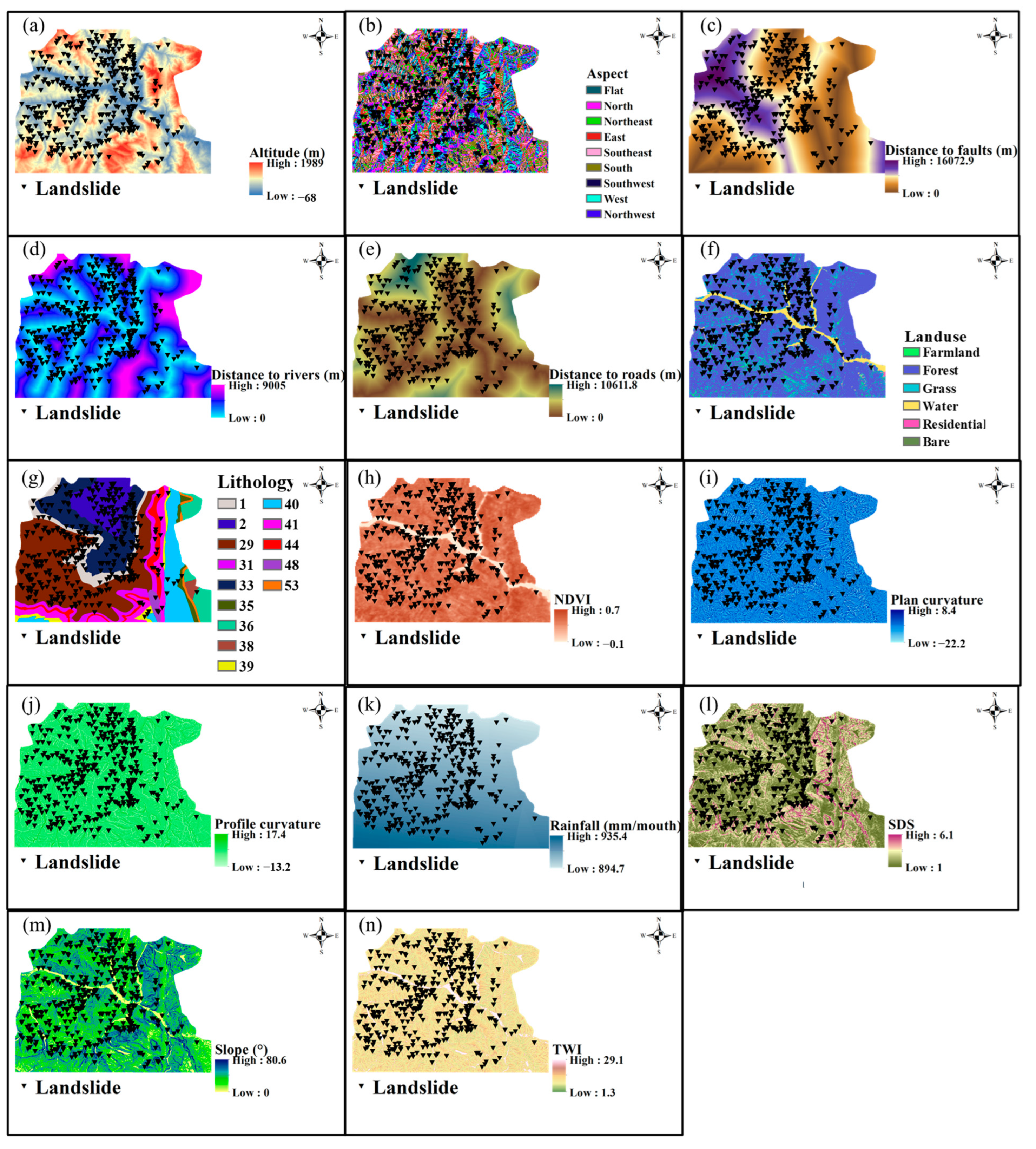
A landslide survey is an indispensable procedure for data statistics and understanding of landslide spatial distribution [22]. The landslide inventories of the study areas were initially obtained from the archive database in 2012 and then were supplemented with several field surveys using geoinformatics (ArcGIS) from Google Earth images (historical images from 2010 to 2016). Additionally, the description of the landslides in the study areas can be found in Table A1 of Appendix A. Figure 1 shows the landslide distribution of the first two study areas. The inventory contains 484 landslide locations in LX and 88 landslide locations in GG. These historical landslide locations are explored by using expert knowledge and onsite investigation, which can be found in the report by the China Geological Environment Monitoring Institute [23]. According to Reichenbach et al. [1], 596 factors have been found to assess landslide susceptibility, from 1983 to 2016, and the average number of factors used in each model is nine. In addition, the selected landslide-influencing factors should be measurable, operable, uneven, complete and nonredundant [24]. Some studies [25,26,27] have shown that using between 4 and 12 factors is suitable for LSP. Therefore, there are 14 landslide-influencing factors (Table 1) are considered in this paper, which can be classified as seven topography factors (altitude, aspect, plan curvature, profile curvature, surface roughness, topographic wetness index and slope), five environmental factors (normalized difference vegetation index, land use, rainfall, distance to rivers and distance to roads) and two geological factors (lithology and distance to faults). The thematic maps of these landslide-influencing factors of LX and GG are shown in Figure 2 and Figure 3, respectively.
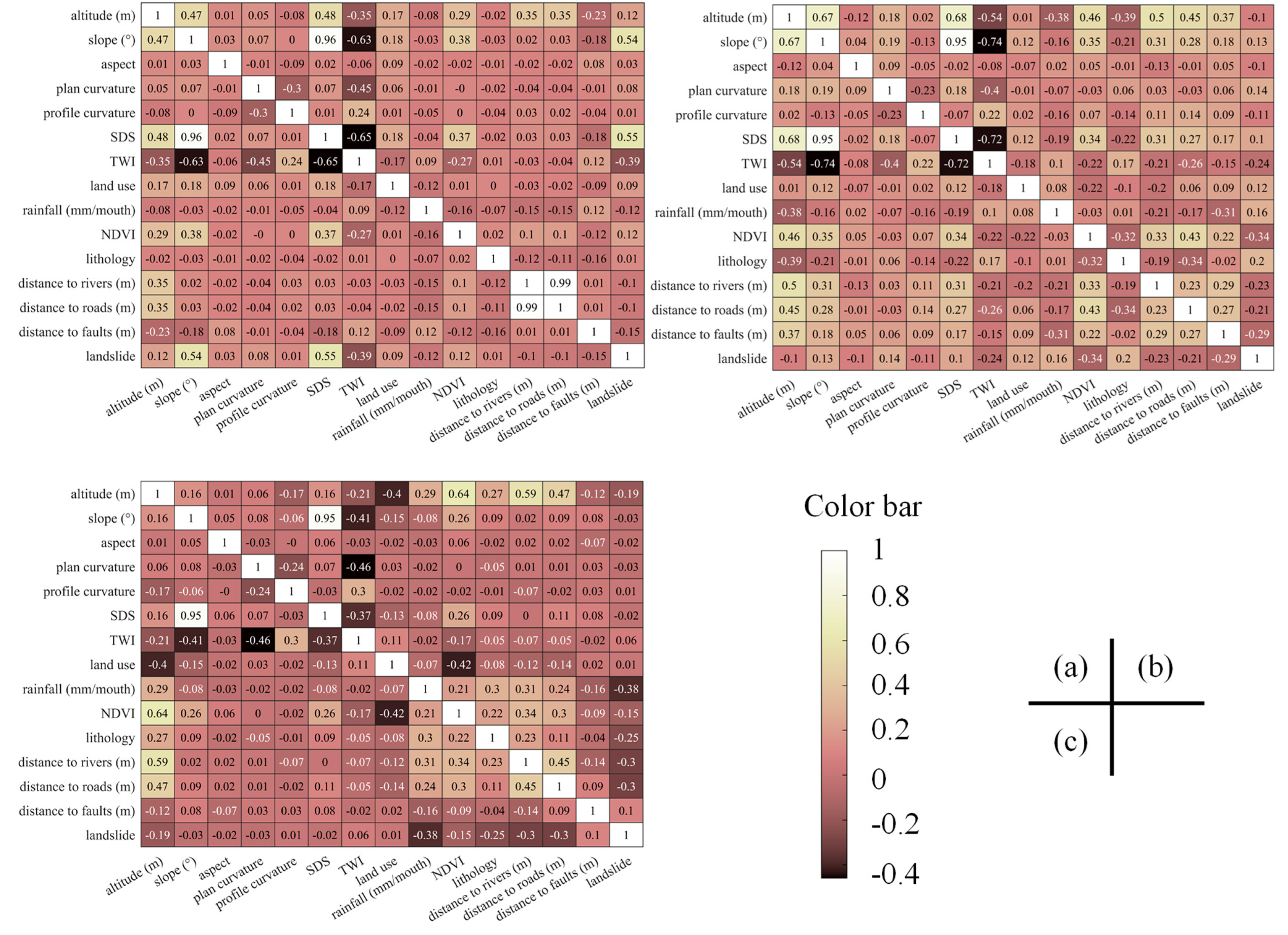
In addition to the positive samples, the same number of negative samples (nonlandslide) are randomly collected from the first two study areas on the basis of following some basic priorities (for example, low slopes) [11,16]. The heat maps of the correlation matrix of the landslide-influencing factors and one output variable for data sets in three study areas are shown in the Figure A1, which illustrates the correlation between parameters. According to the researches [42,43,44], the samples in both areas of this study are split into a training set (80%) and a validation set (20%) for comparison and to validate the performance of each method.

3. Method

3.1. Overview

The paper achieves the transfer learning with attributes for improving model performance in the sample-scarce areas by using a VAEGAN. The method is sketchily shown in Figure 4. First, a VAEGAN is trained from landslide-influencing factors (positive samples and negative samples). Second, the factors with the landslide-related attributes of two areas (LX and GG) will be extracted and reconstructed by a VAE. It is specified in Section 3.4. Finally, the LSP models will be established by a CNN, and the transferability of the models will be tested. The thematic maps of landslide-influencing factors and sample production are made by ArcGIS 10.8 (Environmental Systems Research Institute, Inc., Redlands, CA, USA). Additionally, the deep-learning framework is accomplished on MATLAB 2022a (MathWorks Inc., Native, MA, USA).

3.2. Assessment for Landslide-Influencing Factors

The selection of features is important for the prediction of LSMs [29]. Studies have shown that many factors can be selected [1]. However, redundant features will interfere with the recognition ability of a model, reduce the generalizability and increase the operation time [45]. In order to prove the validity of the selected landslide-influencing factors or eliminate irrelevant factors to improve the predictive ability of the model, the gain ratio (GR) technique [46] is adopted in this paper. When the GR of a factor is less than or equal to zero, the factor is assumed irrelevant to the landslide and should not be used as the input of the model.

3.3. Convolutional Neural Network

As a nonlinear tool that can extract key attributes from large numbers of data [47], the CNNs are used as the LSP model and the feature extractor of a VAEGAN in this paper. In LSP, the CNN input is the landslide-influencing factors in vector format, and the output consists of the landslide (positive class) and nonlandslide (negative class) labels [9,11,48]. In the TLA strategy, the feature extractor of the VAEGANs is a CNN without the classification layer. Furthermore, to avoid numerical problems, the all dimensions of the input data for the LSP model are normalized to [0, 1] by using Equation (1), before being included in the models.
x   r e s c a l e d = x x m i n x m a x x m i n  
where x is the origin input data and x m a x and x m i n are the maximum value and the minimum value of the origin input data, respectively.

3.4. Variational Autoencoder of Generative Adversarial Network

3.4.1. The Training of VAEGANs

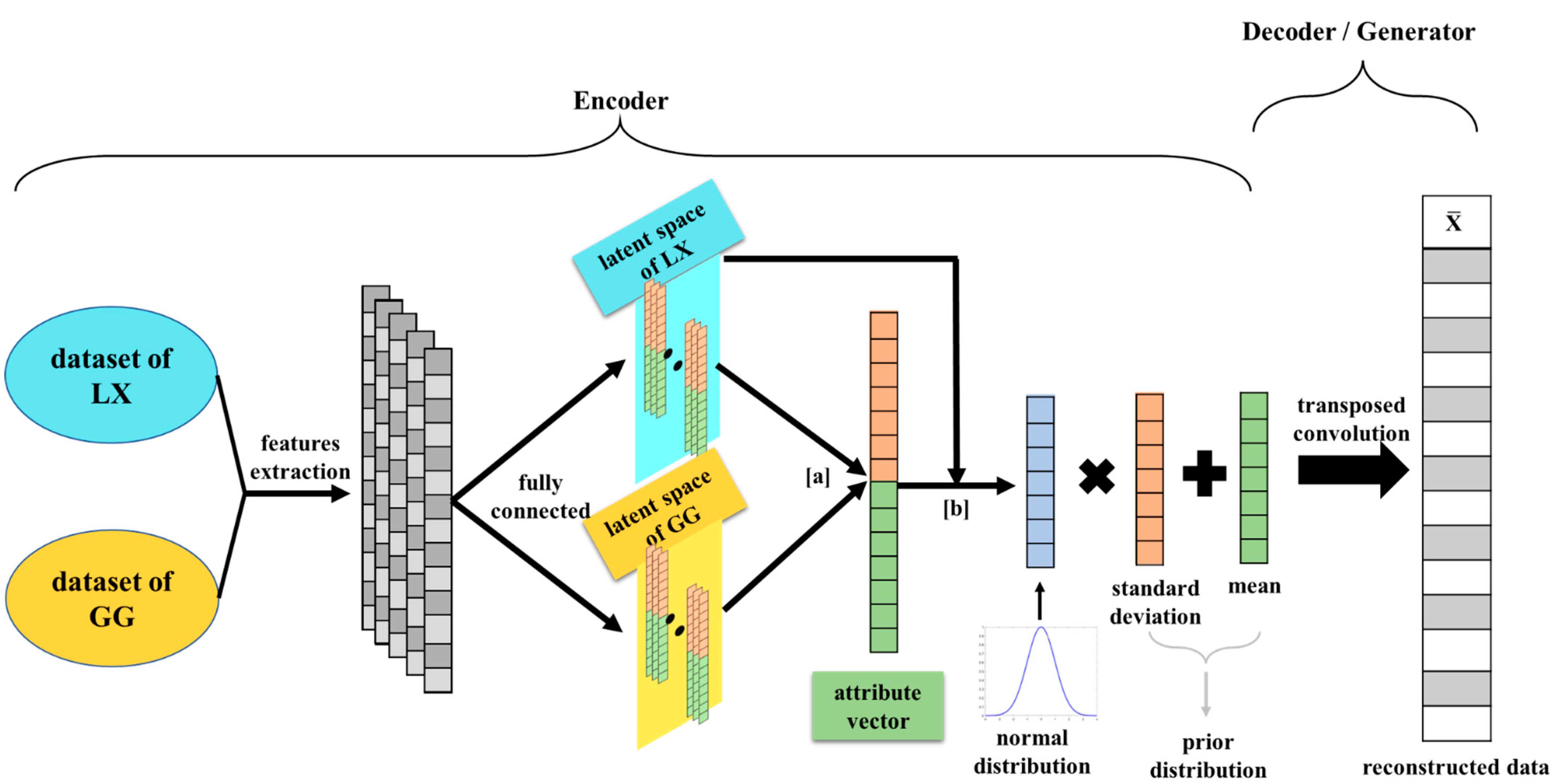
In Figure 5, the VAEGAN has two components: a VAE and a GAN, which share the same generator. Different from regular autoencoders, VAEs apply and learn the probability distribution on the latent space extracted by the encoder from the input, so that the distribution of outputs from the decoder matches that of the observed data. Next, the distribution sampled by the decoder will be encoded to reconstruct new data. Meanwhile, applying a discriminator in the VAE, which is to distinguish whether the data is real or generated, has a positive effect on model performance [21]. The loss of the VAEGAN is shown as follows:
= VAE + GAN
with
VAE = 1 b i = 1 b ( x ¯ i x i ) 2 + [ 0.5   ·   i = 1 b ( 1 + log ( σ i 2 ) μ i 2 σ i 2 ) ]
GAN = i = 1 b ( log ( Dis ( x i ) ) + log ( 1   Dis ( x ¯ i ) ) + log ( 1   Dis ( x p i ) ) )
where b is the minibatch size, x i is the input data, x ¯ i is the reconstructed data decoded from the prior distribution ( z ) and μ i and σ i are the mean and standard deviation (prior distribution) of the latent space, respectively. x p i is the reconstructed data decoded from the normal distribution ( z p ). Dis ( x i ) , Dis ( x ¯ i ) and Dis ( x p i ) comprise the output of the discriminator when the input is the origin data x i , the reconstructed data x ¯ i and the reconstructed data decoded from the normal distribution x p i , respectively.

3.4.2. Data Reconstruction and Transfer Learning with Attributes

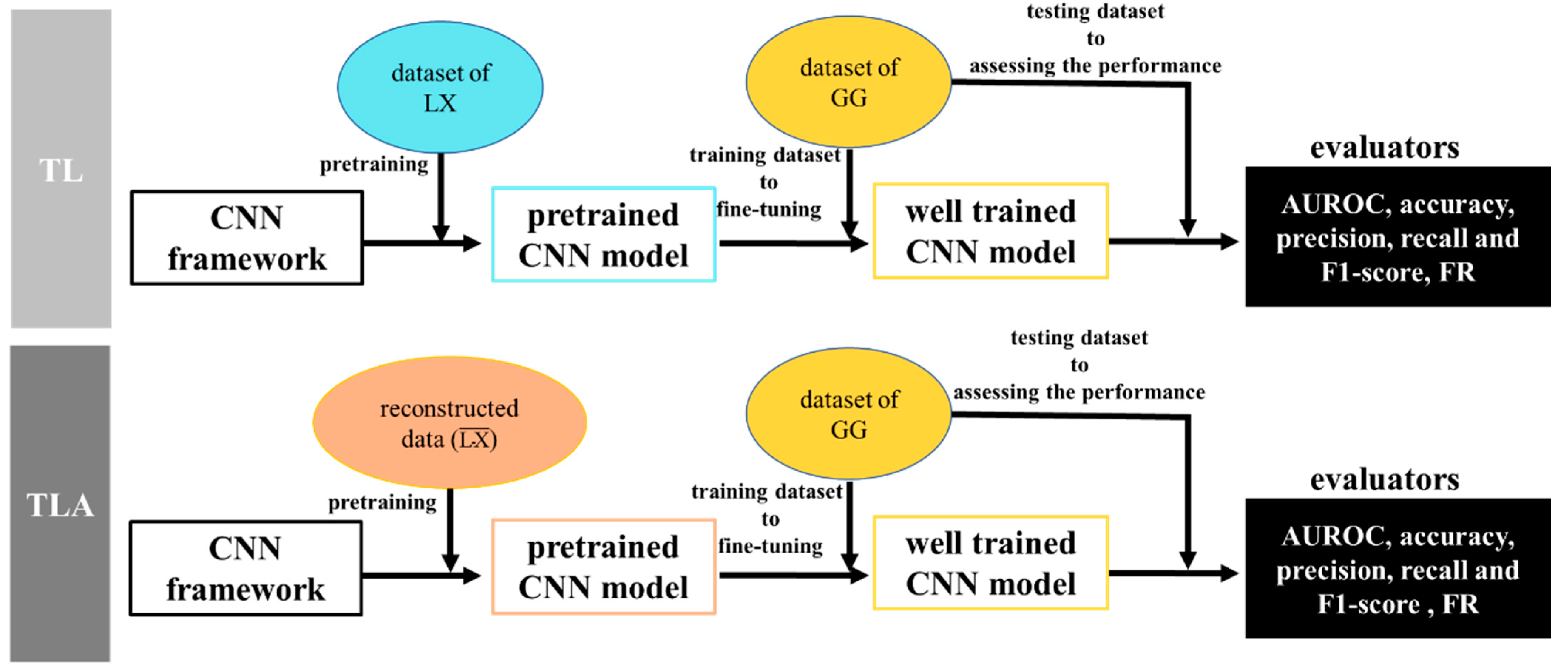
Reconstructing data with attributes can make data with specified knowledge, thereby increasing the commonality and representativity of samples [20]. Specifically, a VAEGAN was pretrained by using the data set of LX and the one of GG. Additionally, the latent vector representations of each data set will be extracted by the pretrained VAEGAN. That is, for each attribute, the mean vectors of the latent space of landslide-influencing factors in each area are computed. Next, the attributes that existed only in a study area (e.g., GG) will be obtained by computing the difference between the mean vectors (operation [a] in Figure 6). Finally, the data containing the attributes of two areas will be obtained by reconstructing the vector, which is the integrated result of the attribute vector (with attributes) and the latent space of LX (without attributes) (operation [b] in Figure 6). The reconstructed data contain the attributes of the landslide-influencing factors in GG and LX, which makes the LSP model learn the attributes beyond one study area. Additionally, the TLA will then be achieved by fine-tuning the model pretrained by the reconstructing data with the labeled samples of GG (Figure 7).

3.5. Evaluators of Model Performance

To investigate the effectiveness of the TLAs strategy, the measures, including accuracy, recall, area under the receiver-operating characteristic (AUROC), precision and the F1-score, are introduced, and their mathematical calculation are listed as follows:
A c c u r a y = T P + T N T P + F P + T N + F N
P r e c i s i o n = T P T P + F P
R e c a l l = T P T P + F N
F 1 s c o r e = 2 × T P 2 × T P + F P + F N
In addition, the landslide-frequency ratio (FR) can be used to assess the model performance even if the landslide susceptibility zones in LSM are varied [29]. The FR is mathematically expressed as:
F R = L A i / T L A A i / T A
where the landslide area of each susceptibility zone is L A i , the total landslide area in the study area is T L A , the area of each susceptibility zone is A i and the total area of the study area is T A . The FR index also considers the relationship between the susceptibility zone in different grades and the landslide area, which indicates the reasonableness of the model to predict the susceptibility zone.

4. Results

4.1. Importance Analysis of Factors

The influencing degree of factors can be reflected by the GR, and the result is shown in Figure 8.
On the one hand, in LX, the topography factors (e.g., SDS and slope) are more important for landslides in this study area than the geological factors (e.g., distance from faults), hydrological factors (e.g., TWI) and environmental factors (e.g., rainfall and land use) are.
On the other hand, in GG, the topography factors (e.g., plan and profile curvature) are more important for landslides than the environmental factors (e.g., rainfall and land use), geological factors (e.g., distance from faults) and hydrological factors (e.g., TWI) are.
In general, the influential extent of these landslide-influencing factors is different in two areas, but the topography factors are most important in the two areas. For example, the SDS and the plan curvature had the highest impact on landslides in LX (0.113) and in GG (0.056), respectively. Thus, all landslide-influencing factors are considered to have a positive impact on landslides.

4.2. Evaluation of Supervised Learning

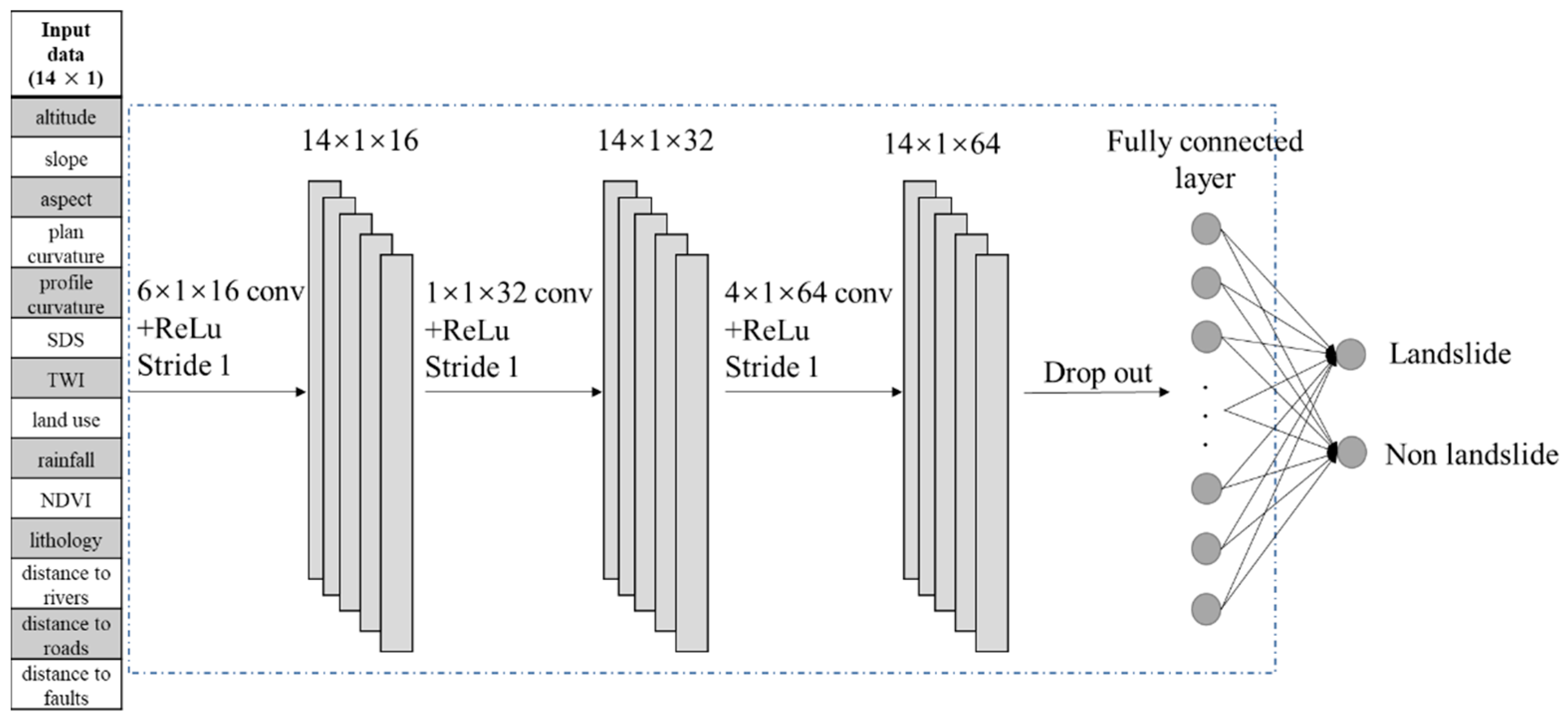
The samples of each study area are randomly divided into 80% and 20% for the training and the validation of the CNN models, respectively. According to Bayesian optimization [49], the best architecture of a CNN features three convolutional layers, no pooling layer and a piecewise decaying learning-rate strategy (Table 2 and Figure 9). This is because the function of the pooling layer is to extract key features from a large amount of information. However, for LSP, when the input dimension is small, adding pooling layers may cause key features to be lost, leading to the opposite of what is expected. For the selection of the learning rate, piecewise decay is better than constant. This indicates that at the later stage of the model iteration, using a small step size is beneficial to search for the smaller value in the loss function.
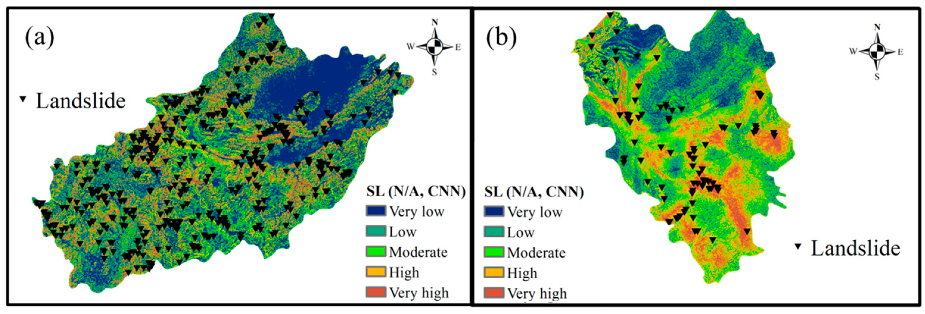
Table 3 is the prediction results of the CNNs with best hyperparameters. The model performance is better when it is trained with the data set of LX. Especially in the AUROC, the model trained with the data set of LX performs better (about 6%) than the one trained with GG. This is because there are sufficient samples in LX. Figure 10 shows the LSMs of two study areas. Additionally, the natural break classification [7] was used to classify landslide susceptibility indices (probability) as very low, low, moderate, high and very high.

4.3. Influence of Transfer Learning with Attribute Strategy on Model Performance

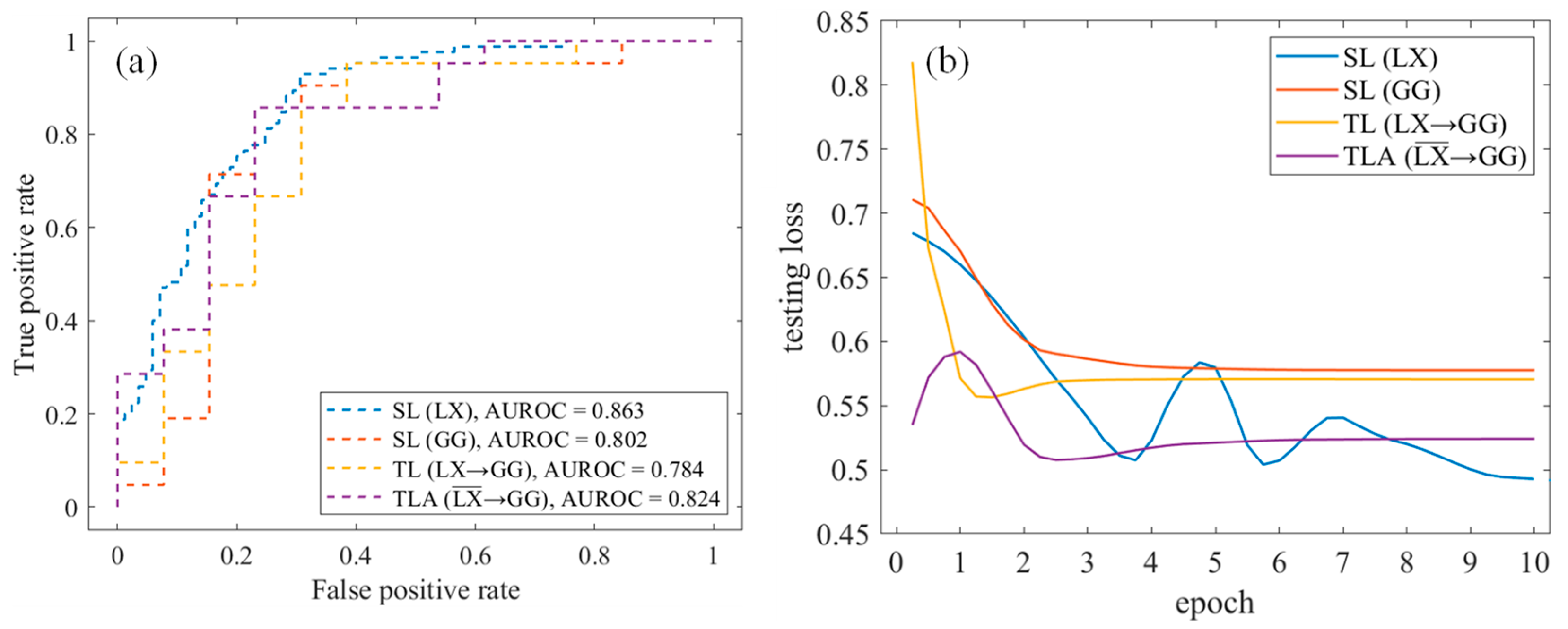
To evaluate the influence of the TLA on model performance, the experiments were implemented, and the results are listed in Table 4. The situation of the training and testing data set is on the left, and the mean value of evaluators (accuracy, AUROC, recall, precision, F1-score) is on the right. No transferring skills are applied in Experiment A; in Experiment B, the GG model is pretrained by the LX data set and fine-tuned with GG-labeled samples. In Experiment C, the GG model is pretrained by the data set with attributes ( L X ¯ ), that are reconstructed by VANs and then fine-tuned with GG-labeled samples.
It can be seen from Experiments A and B that the model performance improved by the TL is inappreciable. It can be seen more clearly from Figure 11a that the model performance actually decreased in AUROC when the TL strategy is applied. Moreover, in the early stage of training (Figure 11b), the loss of the TL strategy is larger than the SL. These results indicate that the sample attributes of the two study areas are quite different and that the model pretrained by LX is not suitable for GG. However, in Experiment C, the model performance is significantly improved by pretraining the model with the data, which were reconstructed by a VAEGAN with a CNN feature extractor. The TLA strategy increased the mean value of evaluators by about 7% compared with the SL and the TL. Meanwhile, in GG, the convergence loss of the TLA is lower than that of the TL and the SL, which indicates that the reconstructed data, L X ¯ , contain the representative of both areas, and the performance of the LSP models in sample-scarce areas can be improved by using the TLA.

5. Discussion

According to the above results, the prediction accuracy of the LSP models was improved by increasing the attribute similarity of the data sets by using the TLA strategy. In order to further explore the transferability of the TLA, the experiments were conducted with different combinations of the LSP models and the feature extractors in the VAEGAN. Additionally, another study area has been employed to assess the transferability of the TLA strategy, which is shown in the following discussion.

5.1. Comparison of LSP Model

The improvement in model performance in the previous section proves the effectiveness of CNN and TLA strategies in establishing LSP models with limited samples. However, different deep-learning models have different effects on evaluators in LSP [50]. Therefore, in order to validate the CNN framework proposed in this paper, the GRU model and the BiLSTM model are added. The hyperparameters and training parameters of these models are obtained by using the Bayesian optimization algorithm.
Table 5 shows the results of LX and GG in supervised learning. It can be seen that all the performance values of the models were decreased in sample-scarce areas, especially the GRU. In the comparisons, the BiLSTM model achieves excellent results in recall and F1-score. Additionally, the CNN is better than the others in AUROC, accuracy and precision, which makes the CNN the best in the mean value of the evaluators.

5.2. Evaluation and Comparison of the Model Transferability

To further explore the performance of the model with the strategy of TLA, this paper proposes the following models: GRU-VAEGAN and BiLSTM-VAEGAN, for example, operation [a] in Figure 5, replace the feature extractors in a VAEGAN from CNN to GRU (experiment D) and BiLSTM (experiment E), respectively. Next, five groups of experiments were conducted.
Table 6 and Figure 12 show the mean values of the above evaluators and ROC curves. When the TLA techniques (in Experiments C, D and E) were used, the performance values of the models are improved, especially the CNN. The best ROC curve of the TLA reaches the highest, 0.844, by comparing those with the SL (0.771) and the TL (0.772).
The loss during training is one of the evaluators reflecting the quality of the data set [19]. The training results are shown in Figure 13. For the LSP models, although GRU converges the fastest, the CNN model has the lowest converging loss. Additionally, BiLSTM is less stable than the others. For transferability (e.g., Figure 13a), the loss is much less in the early training stage when the TLA strategy is used, especially when a CNN is used as VAEGAN feature extractor. This indicates that the TLA technique is effective.
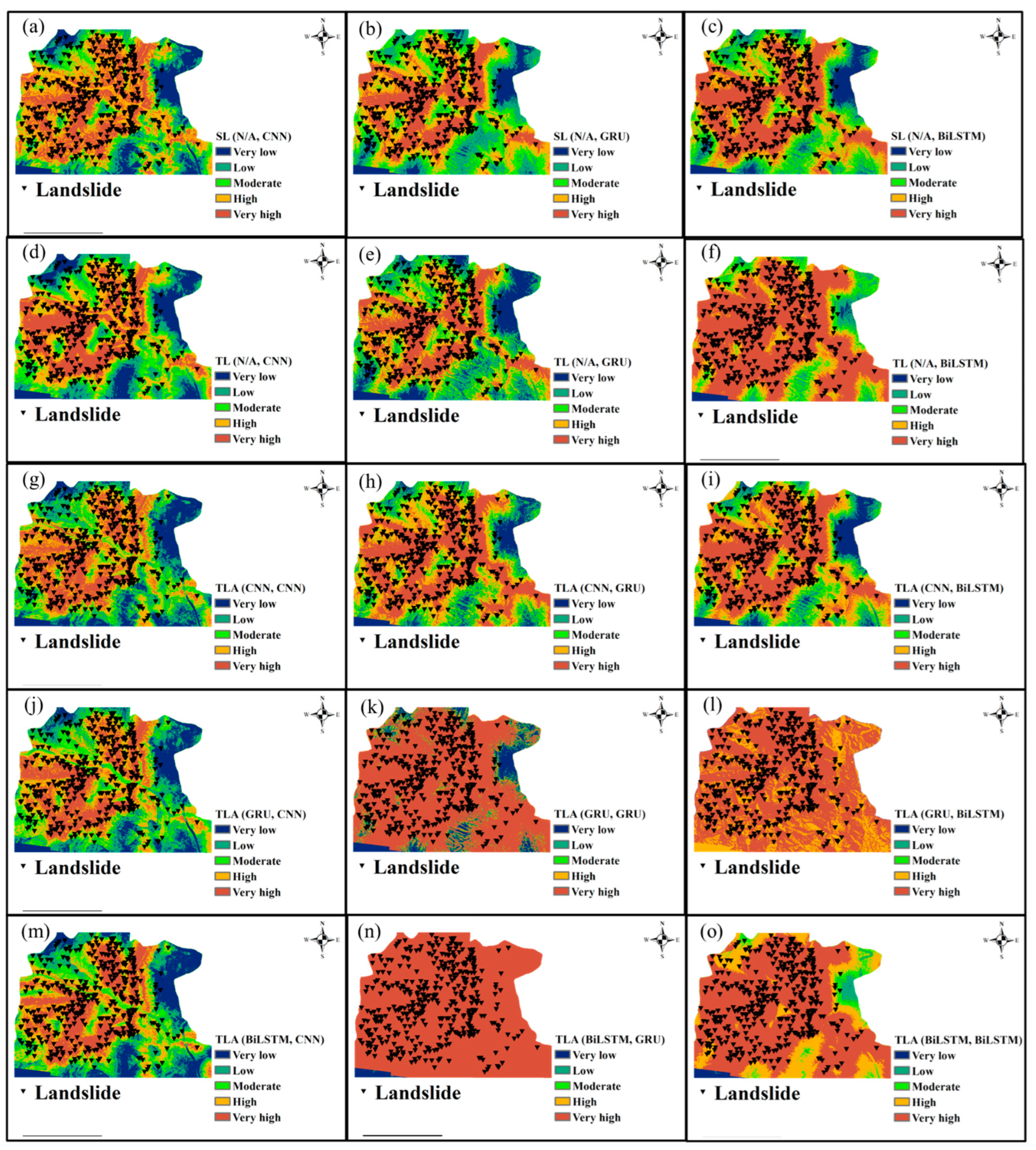
Figure 14 shows the LSMs in GG predicted by models. In Figure 14h,k,n, most grids in the study area are classified as in a very high susceptibility zone, which is inappropriate. It is indicated that the GRU is underfitting when the training samples are inadequate. The model performance seems to be improved by the TLA strategy. In fact, most samples of the testing data set are predicted as the “landslide”, increasing the F1-score and the mean value of evaluators. However, the AUROC and accuracy are poor. This conclusion also can be proved from another aspect. For the data set of the target domain (GG), when reconstructing the data by using a GRU-VAEGAN, the reconstructed data contain little attribute similarity and can even be seen as the noise and can decrease the effect of TLA strategy because of data-set bias. This indicates that the GRU is not a suitable feature extractor of a VAEGAN. In Figure 13a, in case TLA (GRU, CNN), at the beginning, the loss is higher than the losses of the other cases, indicating that the attribute similarity between the data set used to pretrain the model and the one of target domain is minor. The loss converges to a lower value because of the strong fitting ability of the CNN.
The LSMs of well-trained models should have higher landslide-density values (frequency ratios) in very high susceptibility zones than in other ones [29]. To qualitatively evaluate the model performance values, the FR method was used; the FR values in the high and very high susceptibility zones of each situation are shown in Figure 15. For the LSP models, the high and very high landslide susceptibility zones predicted by the CNN contained 75% of the historical landslides but only accounted for about 30% of the total area, reaching the highest FR value by comparing them with GRU and BiLSTM. For transferability, Figure 15b–d shows the FRs when the LSP model is the CNN, GRU and BiLSTM, respectively. Additionally, it can be concluded that compared with the SL and the TL, the TLA strategy can significantly improve the performance of an LSP model.

5.3. Application of Transfer Learning with Attribute in Other Study Area

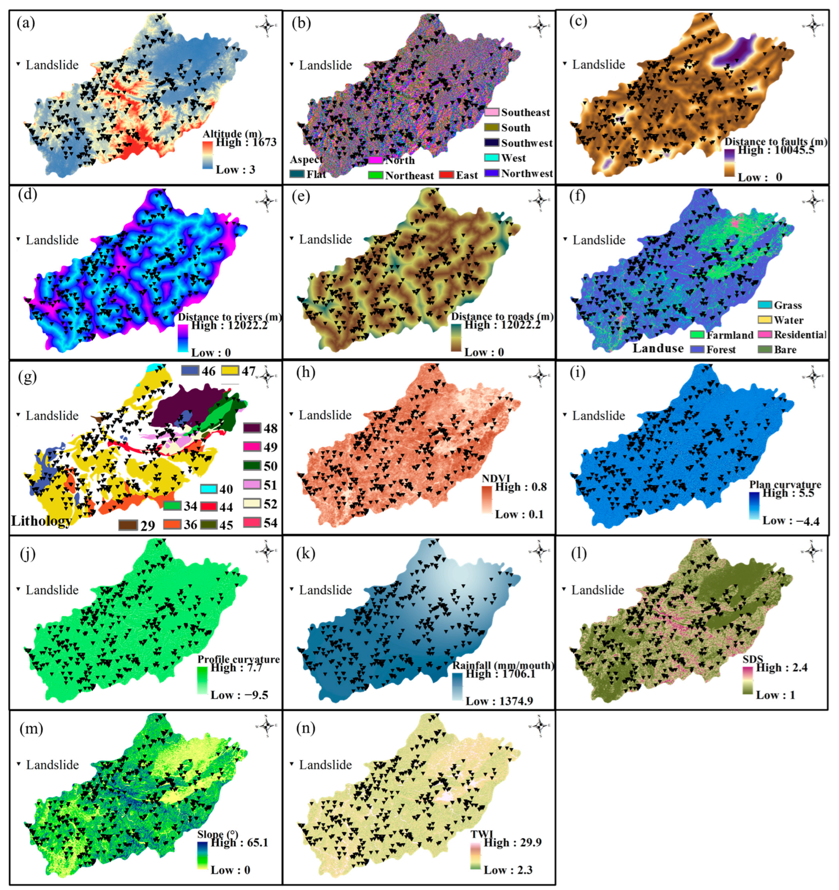
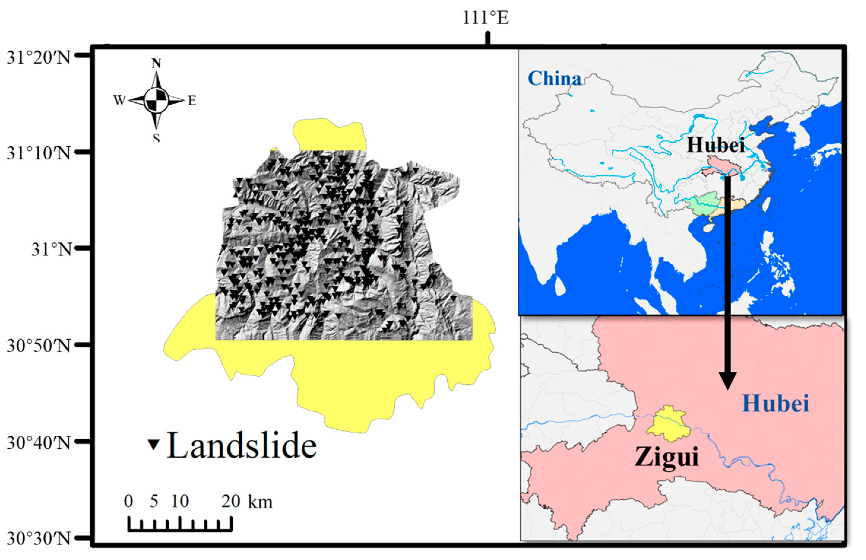
In order to further investigate the transferability of the TLA strategy between the areas with huge differences, Zigui County, Hubei Province, China, was added. Zigui County is located in the Three Gorges Reservoir Area (TGRA) of the Yangtze River Basin. Data on 409 historical landslides, as shown in Figure 16, were obtained from the landslide inventory. Additionally, the thematic maps of Zigui County can be found in Figure A2 of Appendix A.
The performed experiments are consistent with the previous ones, and the results are shown in Table 7 and Table 8. The AUROC is shown in Figure 17. In the SL, the CNN achieves the best results in evaluators. However, the CNN is also more sensitive to the data set with or without the attributes than the others. In Table 8, when the TL was applied, only the CNN model performance values decrease. This is because the distance between the two places is large, so the attributes of landslide-influencing factors are different (e.g., lithology and rainfall). Applying the TL strategy between the data sets with huge differences will reduce the model performance because the differences will be considered as noise for model training. However, the reconstructed data contain the attributes of both study areas; thus, the model performance values are increased when applying the TLA strategy.
The Figure 18 shows the training process of the models. As before, the BiLSTM takes longer convergence time and is less stable compared with the CNN and GRU. Furthermore, when the TLA technique is used, the training progress is more efficient and yields a lower convergence loss.
The LSMs of ZG predicted by the models are shown in Figure A3 of Appendix A. It can be seen that the LSMs predicted by GRU and BiLSTM contained more high and very high susceptibility zones compared to the CNN. Figure 19 shows the FRs in different situations, and this information helps to more clearly evaluate the rationality of these LSMs and the transferability of these techniques (TL and TLA). The model performance is improved by using the TLA, especially by pretraining the LSP models (the CNN) with the data reconstructed by the CNN-VAEGAN, indicating that the TLA strategy has strong compatibility regardless of the far distance between ZG and LX.
The evaluation of the models showed that the proposed TLA strategy can improve the performance of the LSP model in both GG and ZG. When the TLA strategy was applied, the evaluators of all the models were improved. Moreover, different feature extractor of the VAEGAN significantly affected the transferability in LSP. The reconstructed data contain more similar attributes of both study areas and improve the transferability when the feature extractor of the VAEGAN is a CNN, which facilitates efficient and reliable prediction in the sample-scarce area.

5.4. Findings and Limitations of This Study

At present, there are also some outstanding studies that have contributed to improving model performance in landslide susceptibility mapping [51], building damage assessment after earthquakes [52] and flood assessment [53] by applying the TL strategy. Unlike these studies, which directly gather knowledge from previous, similar situations (known as case-based reasoning) or select the data from a source area that has a similar distribution to the target area (known as domain adaptation) to complete the TL strategy, this study proposes the TLA strategy, which increases the attribute similarity between the source and target domain data sets. The TLA strategy achieves this by reconstructing the data of the source area according to the attributes of both the source area and the target area. Compared with case-based reasoning, the TLA strategy improves model performance in scarce-sample areas and achieves better prediction results. The goals of both domain adaptation and the TLA are to enhance model performance by using the samples that are more similar to the target domain distribution. However, the domain adaptation focuses more attention on selecting the similar distribution data from source domain, while the proposed TLA strategy reconstructs the source domain samples by using the VAEGAN to generate the data with attributes similar to those of the target domain. The comparisons of these two strategies in sample-scare areas deserve further investigation in future research.
To further explore the effect of sample size on the TLA strategy, several experiments were conducted in the GG and ZG study areas.
The GG study areas were assumed to have only 11, 22, 33, 44, 55, 66, 77 and 88 samples, separately. In each case, the samples were randomly selected from the landslide inventory, and the training and test data sets were divided in the ratio of 4:1. As shown in Figure 20, the model performance values are improved by increasing the number of training samples. Additionally, the LSP model yielded the best performance with 22 samples by applying the TLA strategy, compared to the SL and the TL.
Similarly, the ZG study areas were assumed to have only 51, 102, 153, 204, 255, 306, 357 and 409 samples, separately. As shown in Figure 21, the model performance was lower when the TL strategy was applied with a sample size of 102, compared to the SL. However, the model performance reached 0.809 at the mean value of evaluators by applying the TLA strategy, which exceeded the performance of the SL (0.796) and TL (0.734) strategies.
This study found out that the transferability of the TLA is also affected by the distance between the study areas. Compared to GG, the application of the TL strategy in ZG is less effective than the SL owing to the increase in the distance between the source and target domains, resulting in a greater difference in the attribute similarity of the landslide-influencing factors. The smaller the distance between the study areas (e.g., LX and GG), the more obviously the TLA strategy can improve the performance of the model. Although the increase in the distance reduces the similarity between the data sets (e.g., LX and ZG), the TLA strategy can still to some extent improve the performance of the model, which demonstrates the robustness of the proposed TLA strategy.
In summary, this parametric study shows that to obtain a reasonable landslide spatial model by using the TLA strategy, at least 55 and 102 properly selected sample points are required for the GG and ZG test data sets, respectively. These sample points resulted in a mean evaluator value of 0.762 and 0.809 for the GG and ZG test data sets, respectively.
Meanwhile, the proposed TLA also has the following limitations:
  • As the landslide prediction model in this study is limited to a deep-learning framework, hybrid deep-learning methods (e.g., hybrid deep-learning frameworks, hybrid deep-learning–machine-learning frameworks) are worth trying in order to improve the reliability and accuracy of LSMs.
  • Regarding the lack of considerations of the landslide range and spatial information, the landslide inventory in this paper consists of single points, which limits the input of LSP models limited to the 1D sequence format. The prospective research can focus on combining the information of remote-sensing images and explore the feature processing ability of CNNs in high-dimensional (landslide pixel spatial) data.

6. Conclusions

For the first time, the present study proposed a TLA strategy that was based on the VAEGAN models (CNN-VAEGAN, GRU-VAEGAN and BiLSTM-VAEGAN) in LSP, which can facilitate and expedite the training progress with limited landslide samples. The main conclusions were as follows:
  • The CNN frameworks were not only an excellent selection for the LSP model but also a worthwhile choice for a feature extractor for a VAEGAN in TLAs.
  • For the LSP in the SL strategy, the performance of the CNN was more reliable than that of the BiLSTM and GRU, which achieved the best performance in the mean value of evaluators (AUROC, accuracy, precision, recall, F1-score and FR) in three study areas.
  • For the transferability, the TLAs strategy developed in this research yielded better results in performance of landslide prediction models in sample-scarce areas, which surpassed the TL, reflecting the practicability and advantage of the methods proposed in this paper.

Author Contributions

M.L. contributed to the conceptualization, methodology, investigation, original draft preparation and data curation of the paper. S.T. contributed to the investigation, original draft preparation and supervision of the paper. G.C. contributed to the investigation, review and editing of the paper. D.B. contributed to the review of the paper. All authors have read and agreed to the published version of the manuscript.

Funding

This research received no external funding.

Data Availability Statement

The landslide-influencing factors, thematic maps of the study areas and LSMs were extracted and processed by ArcGIS 10.8. The paper used MATLAB 2022a to reconstruct the data with attributes. The main code is shown in the following link: https://github.com/linmmsbaby/TLAs (accessed on 18 October 2022).

Conflicts of Interest

The authors declare no conflict of interest.

Appendix A

Table A1. Description of the landslides in the study area.
Study AreaLandslide TypeCausation
LXMostly, the landslides are the small- and medium-scale falls. Additionally, there are the small-scale creeps and earth flows.Human engineering activities (e.g., house building, road construction, canal construction and mining) and heavy rainfall.
GGMostly, the landslides are the medium- and large-scale falls. There are also small-scale creeps.Landslides of soil slopes are caused by the erosion of concave and convex banks during the rainy season. The geology and topography (e.g., isolated peaks, tectonic fissures and solution fissures development section with poor vegetation development) are the main reasons for the landslides on rocky slopes.
ZGMostly, the landslides are the medium- and large-scale creeps. There are also small-scale falls and earth flows.The main reason for the creep is geological (the rocks and soils are multidimensional gravelly soils, with a loose structure and easy permeability). Additionally, the falls are related mainly to heavy rainfall and human activities such as mining.
Note: The scale ( × 10 4 m3) in landslide: large scale (100 to 1000), medium scale (10 to 100) and small scale (less than 10); the fall: large scale (10 to 100), medium scale (1 to 10) and small scale (less than 1); earth flow: large scale (20 to 50), medium scale (2 to 20) and small scale (less than 2).
Table A2. Description of the lithological formations in the study areas.
#SymbolUnit NameDescription
1 J 1 Ziliujing Formation, Xintiangou FormationPurple-red mudstone, sandstone, siltstone, conglomerate, shale and mudstone.
2 J 3 Suining FormationRed mudstone (or siltstone) with interbedded conglomerate and sandstone clasts.
29 T 3 Xiaoyunwushan FormationThick beds of quartz sandstone, conglomerate sandstone with interbedded gravel, sand and gravel, carbonaceous shale, coal seams and thin beds of coal.
31 P 1 Nandan Formation, Maping FormationGrayish-white clayey siltstone, microcrystalline limestone, bioclastic limestone and dolomitic limestone.
32 P 2 - 3 Heshan-longtan Formation, Sidazhai Formation, Gufeng Formation, Xixia FormationGraywacke, mudstone, sandstone, siliceous rock, shale with interbedded coal seams.
33 J 3 Shaximiao Formation, Qianfoya FormationThe lower part is dominated by fine-grained sandstone and shale with interbedded bands of mudstone and the bottom contains fine gravel. The upper part is characterized by alternating layers of mudstone and conglomeratic sandstone.
34NhDaganshan FormationQuartz-muscovite schist, muscovite-quartz schist, quartzite interbedded with carbonaceous phyllite, siliceous rock, shale, tuffaceous shale and layers of pyrite, with the base being quartzite interbedded with gravel.
35ZDoushantuo Formation, Dengying FormationCarbonaceous or phosphorite-siliceous dolomitic limestone and shale interbedded with carbonaceous shale and siliceous layers, and middle to thick-bedded to massive carbonate rock.
36 γ m i P t 3 Paleozoic mixed rockTwo-mica granite derived from the original mixed rock.
38 A r 3 Kongling group (including Xiaoyicun Formation and Gucunping Formation)The lower group consists mainly of black biotite schist, while the upper group is a combination of graphitic schist, marble, calcium-silicate rock and quartzite.
39ONanjingguan Formation, Honghuayuan Formation, Dawan Formation, Guniu Formation, Miaopo Formation, Baota FormationComposed mainly of bioclastic limestone, limestone, nodular fossiliferous limestone, calcareous shale and shale with interbedded shale.
40 3 Shuishi FormationComplex rhythmic layer of altered sandstone and shale and carbonaceous shale.
41 S 1 - 2 Xintan Formation, Luoreping Formation, Shamao Formation The main composition consists of yellow-green and gray-green thin layers of fine-grained sandy clay (siltstone) and muddy sandstone, with small amounts of fine sandstone and greywacke, mudstone interbedded. The sandstone increases in thickness in the upper part.
44 D 2 Guitou group (including Yangxi Formation and Laohutou Formation)Lower part consists of gravel, sand and gravel interbedded with sandstone, siltstone; upper part consists of quartz-rich gravel, conglomerate with gravel and sand, quartz sandstone, siltstone and siltstone with shale.
45 D 3 Maozifeng Formation, Changtuduo Formation, Dasai FormationCalcareous siltstone, siltstone with sandstone beds, bioclastic limestone and sandstone with shale beds.
46 γ π k 2 Late Cretaceous granodioriteGranite porphyry.
47 γ O 2 Middle Ordovician graniteGranular black mica granite with coarse and medium-sized grains.
48 K 2 Sanyajiang FormationVolcanic breccia, sandstone, siltstone, tuffaceous greywacke, rhyolite tuff, rhyolite, andesitic tuffaceous greywacke, andesite, pumice and lava flows.
49 ψ o P t 3 Paleozoic hornblende rockSplaying Schistose Gneiss.
50 C 1 Shidengzi Formation, Ceshui Formation, Xinmenqiao Formation, Dasaiba FormationThick layer of limestone, interbedded limestone, shale, sandstone, limestone, carbonate limestone, coal seams, shale-interbedded sandy mudstone and shale.
51 C 1 Ceshui FormationThe main composition is quartz sandstone and fine sandstone, interbedded with black shale and non-smoldering coal beds. In some local areas there are interbedded limestones and mudstones.
52 Qh f Dawanzhen FormationSand and gravel interbedded with clayey sand.
53NhLiantuo Formation, Nantuo FormationMainly grey-white, grey-green, purple-red sandstone and conglomerate, with conglomerate at the base; grey-green, purple-red to conglomeratic rock.
54JxQbYunkai group (including Fengdongkou Formation, Lankeng Formation and Shawanping Formation)A group of metamorphic rocks containing a complex of metamorphic volcanic rocks, metamorphic iron and phosphate mineral layers.
Figure A1. The heat maps of the correlation matrix of the landslide-influencing factors and one output variable for data sets in (a) LX, (b) GG and (c) ZG.
Land 12 00525 g0a1
Figure A2. Thematic maps of the Zigui County: (a) altitude, (b) aspect, (c) distance to faults, (d) distance to rivers, (e) distance to roads, (f) land use, (g) lithology, (h) NDVI, (i) plan curvature, (j) profile curvature, (k) rainfall, (l) SDS, (m) slope, (n) TWI.
Land 12 00525 g0a2
Figure A3. LSM of ZG using (ac) SL, (df) TL and (go) TLA.
Land 12 00525 g0a3

References

  1. Reichenbach, P.; Rossi, M.; Malamud, B.D.; Mihir, M.; Guzzetti, F. A review of statistically-based landslide susceptibility models. Earth-Sci. Rev. 2018, 180, 60–91. [Google Scholar] [CrossRef]
  2. Liu, Y.; Xu, C.; Huang, B.; Ren, X.W.; Liu, C.Q.; Hu, B.D.; Chen, Z. Landslide displacement prediction based on multi-source data fusion and sensitivity states. Eng. Geol. 2020, 271, 105608. [Google Scholar] [CrossRef]
  3. Wang, H.J.; Xiao, T.; Li, X.Y.; Zhang, L.L.; Zhang, L.M. A novel physically-based model for updating landslide susceptibility. Eng. Geol. 2019, 251, 71–80. [Google Scholar] [CrossRef]
  4. Park, J.Y.; Lee, S.R.; Lee, D.H.; Kim, Y.T.; Lee, J.S. A regional-scale landslide early warning methodology applying statistical and physically based approaches in sequence. Eng. Geol. 2019, 260, 105193. [Google Scholar] [CrossRef]
  5. Lin, S.; Zheng, H.; Han, B.; Li, Y.Y.; Han, C.; Li, W. Comparative performance of eight ensemble learning approaches for the development of models of slope stability prediction. Acta Geotech. 2022, 17, 1477–1502. [Google Scholar] [CrossRef]
  6. Lee, J.-H.; Sameen, M.I.; Pradhan, B.; Park, H.-J. Modeling landslide susceptibility in data-scarce environments using optimized data mining and statistical methods. Geomorphology 2018, 303, 284–298. [Google Scholar] [CrossRef]
  7. Chen, W.; Pourghasemi, H.R.; Naghibi, S.A. A comparative study of landslide susceptibility maps produced using support vector machine with different kernel functions and entropy data mining models in China. Bull. Eng. Geol. Environ. 2017, 77, 647–664. [Google Scholar] [CrossRef]
  8. Sun, D.L.; Wen, H.J.; Wang, D.Z.; Xu, J.H. A random forest model of landslide susceptibility mapping based on hyperparameter optimization using Bayes algorithm. Geomorphology 2020, 362, 107201. [Google Scholar]
  9. Wang, Y.; Fang, Z.; Hong, H. Comparison of convolutional neural networks for landslide susceptibility mapping in Yanshan County, China. Sci. Total Environ. 2019, 666, 975–993. [Google Scholar] [CrossRef]
  10. Krizhevsky, A.; Sutskever, I.; Hinton, G.E. ImageNet classification with deep convolutional neural networks. Commun. ACM 2017, 60, 84–90. [Google Scholar]
  11. Hakim, W.L.; Rezaie, F.; Nur, A.S.; Panahi, M.; Khosravi, K.; Lee, C.W.; Lee, S. Convolutional neural network (CNN) with metaheuristic optimization algorithms for landslide susceptibility mapping in Icheon, South Korea. J. Environ. Manag. 2022, 305, 114367. [Google Scholar] [CrossRef]
  12. He, Y.; Zhao, Z.A.; Yang, W.; Yan, H.W.; Wang, W.H.; Yao, S.; Zhang, L.F.; Liu, T. A unified network of information considering superimposed landslide factors sequence and pixel spatial neighbourhood for landslide susceptibility mapping. Int. J. Appl. Earth Obs. Geoinf. 2021, 104, 102508. [Google Scholar] [CrossRef]
  13. Wang, H.J.; Zhang, L.M.; Luo, H.Y.; He, J.; Cheung, R.W.M. AI-powered landslide susceptibility assessment in Hong Kong. Eng. Geol. 2021, 288, 106103. [Google Scholar] [CrossRef]
  14. Yi, Y.N.; Zhang, Z.J.; Zhang, W.C.; Jia, H.H.; Zhang, J.Q. Landslide susceptibility mapping using multiscale sampling strategy and convolutional neural network: A case study in Jiuzhaigou region. Catena 2020, 195, 104851. [Google Scholar] [CrossRef]
  15. Yang, Y.; Yang, J.T.; Xu, C.D.; Xu, C.; Song, C. Local-scale landslide susceptibility mapping using the B-GeoSVC model. Landslides 2019, 16, 1301–1312. [Google Scholar] [CrossRef]
  16. Zhu, Q.; Chen, L.; Hu, H.; Pirasteh, S.; Li, H.F.; Xie, X. Unsupervised Feature Learning to Improve Transferability of Landslide Susceptibility Representations. IEEE J. Sel. Top. Appl. Earth Obs. Remote Sens. 2020, 13, 3917–3930. [Google Scholar] [CrossRef]
  17. Al-Najjar, H.A.H.; Pradhan, B. Spatial landslide susceptibility assessment using machine learning techniques assisted by additional data created with generative adversarial networks. Geosci. Front. 2021, 12, 625–637. [Google Scholar] [CrossRef]
  18. Lei, H.J.; Han, T.; Zhou, F.; Yu, Z.; Qin, J.; Elazab, A.; Lei, B.Y. A deeply supervised residual network for HEp-2 cell classification via cross-modal transfer learning. Pattern Recognit. 2018, 79, 290–302. [Google Scholar] [CrossRef]
  19. Zhuang, F.Z.; Duan, K.Y.; Xi, D.B.; Zhu, Y.C.; Zhu, H.S.; Xiong, H.; He, Q. A Comprehensive Survey on Transfer Learning. Proc. IEEE 2021, 109, 43–76. [Google Scholar] [CrossRef]
  20. Deng, W.J.; Zheng, L.; Ye, Q.X.; Kang, G.L.; Yang, Y.; Jiao, J.B. Image-Image Domain Adaptation with Preserved Self-Similarity and Domain-Dissimilarity for Person Re-identification. arXiv 2017, arXiv:1512.09300v2. [Google Scholar]
  21. Larsen, A.B.L.; Sønderby, S.K.; Larochelle, H.; Winther, O. Autoencoding beyond pixels using a learned similarity metric. arXiv 2016, arXiv:1711.07027v3. [Google Scholar]
  22. Tian, Y.Y.; Xu, C.; Ma, S.Y.; Xu, X.W.; Wang, S.Y.; Zhang, H. Inventory and Spatial Distribution of Landslides Triggered by the 8th August 2017 MW 6.5 Jiuzhaigou Earthquake, China. J. Earth Sci. 2018, 30, 206–217. [Google Scholar] [CrossRef]
  23. Li, Y.; Yang, X.D.; Fang, H.; Yin, C.R.; Qu, X.Y. Zoning Atlas of Geological Disaster Susceptibility Levels in Typical Counties (Cities) in China; Science Press: Beijing, China, 2012. [Google Scholar]
  24. Ayalew, L.; Yamagishi, H. The application of GIS-based logistic regression for landslide susceptibility mapping in the Kakuda-Yahiko Mountains, Central Japan. Geomorphology 2005, 65, 15–31. [Google Scholar] [CrossRef]
  25. Huang, F.M.; Cao, Z.S.; Guo, J.F.; Jiang, S.H.; Li, S.; Guo, Z.Z. Comparisons of heuristic, general statistical and machine learning models for landslide susceptibility prediction and mapping. Catena 2020, 191, 104580. [Google Scholar] [CrossRef]
  26. Aditian, A.; Kubota, T.; Shinohara, Y. Comparison of GIS-based landslide susceptibility models using frequency ratio, logistic regression, and artificial neural network in a tertiary region of Ambon, Indonesia. Geomorphology 2018, 318, 101–111. [Google Scholar] [CrossRef]
  27. Chang, Z.L.; Du, Z.; Zhang, F.; Huang, F.M.; Chen, J.W.; Li, W.B.; Guo, Z.Z. Landslide Susceptibility Prediction Based on Remote Sensing Images and GIS: Comparisons of Supervised and Unsupervised Machine Learning Models. Remote Sens. 2020, 12, 502. [Google Scholar] [CrossRef] [Green Version]
  28. Lin, M.S.; Teng, S.; Chen, G.F.; Hu, B. Application of convolutional neural networks based on Bayesian optimization to landslide susceptibility mapping of transmission tower foundation. Bull. Eng. Geol. Environ. 2023, 82, 51. [Google Scholar] [CrossRef]
  29. Guo, Z.Z.; Shi, Y.; Huang, F.M.; Fan, X.M.; Huang, J.S. Landslide susceptibility zonation method based on C5.0 decision tree and K-means cluster algorithms to improve the efficiency of risk management. Geosci. Front. 2021, 12, 101249. [Google Scholar] [CrossRef]
  30. Pham, B.T.; Bui, D.T.; Indra, P.; Dholakia, M.B. Landslide Susceptibility Assessment at a Part of Uttarakhand Himalaya, India using GIS-based Statistical Approach of Frequency Ratio Method. Int. J. Eng. Res. Technol. 2015, 4, 338–344. [Google Scholar]
  31. Oh, H.J.; Pradhan, B. Application of a neuro-fuzzy model to landslide-susceptibility mapping for shallow landslides in a tropical hilly area. Comput. Geosci. 2011, 37, 1264–1276. [Google Scholar] [CrossRef]
  32. Wu, Y.L.; Ke, Y.T.; Chen, Z.; Liang, S.Y.; Zhao, H.L.; Hong, H.Y. Application of alternating decision tree with AdaBoost and bagging ensembles for landslide susceptibility mapping. Catena 2020, 187, 104396. [Google Scholar] [CrossRef]
  33. Atkinson, P.M.; Massari, R. Generalised linear modelling of susceptibility to landsliding in the central apennines, Italy. Comput. Geosci. 1998, 24, 373–385. [Google Scholar] [CrossRef]
  34. Moore, I.D.; Grayson, R.B.; Ladson, A.R. Digital terrain modelling: A review of hydrological, geomorphological, and biological applications. Hydrol. Process. 1991, 5, 3–30. [Google Scholar] [CrossRef]
  35. Pham, B.T.; Bui, D.T.; Prakash, I.; Dholakia, M.B. Rotation forest fuzzy rule-based classifier ensemble for spatial prediction of landslides using GIS. Nat. Hazards 2016, 83, 97–127. [Google Scholar] [CrossRef]
  36. Gong, P.; Liu, H.; Zhang, M.N.; Li, C.C.; Wang, J.; Huang, H.B.; Clinton, N.; Ji, L.Y.; Li, W.Y.; Bai, Y.Q.; et al. Stable classification with limited sample: Transferring a 30-m resolution sample set collected in 2015 to mapping 10-m resolution global land cover in 2017. Sci. Bull. 2019, 64, 370–373. [Google Scholar] [CrossRef] [Green Version]
  37. Pham, B.T.; Bui, D.T.; Dholakia, M.B.; Prakash, I.; Pham, H.V. A Comparative Study of Least Square Support Vector Machines and Multiclass Alternating Decision Trees for Spatial Prediction of Rainfall-Induced Landslides in a Tropical Cyclones Area. Geotech. Geol. Eng. 2016, 34, 1807–1824. [Google Scholar] [CrossRef]
  38. Bui, D.T.; Hoang, N.D. A Bayesian framework based on a Gaussian mixture model and radial-basis-function Fisher discriminant analysis (BayGmmKda V1.1) for spatial prediction of floods. Geosci. Model Dev. 2017, 10, 3391–3409. [Google Scholar]
  39. Arabameri, A.; Chen, W.; Loche, M.; Zhao, X.; Li, Y.; Lombardo, L.; Cerda, A.; Pradhan, B.; Bui, D.T. Comparison of machine learning models for gully erosion susceptibility mapping. Geosci. Front. 2020, 11, 1609–1620. [Google Scholar] [CrossRef]
  40. Dwyer, J.; Schmidt, G. The MODIS Reprojection Tool. In Earth Science Satellite Remote Sensing; Qu, J.J., Gao, W., Kafatos, M., Murphy, R.E., Salomonson, V.V., Eds.; Springer: Berlin/Heidelberg, Germany, 2006. [Google Scholar]
  41. Li, C.Y.; Wang, X.C.; He, C.Z.; Wu, X.; Kong, Z.Y.; Li, X.L. National 1:200,000 Digital Geological Map (Public Edition) Spatial Database. Geol. China 2019, 46, 1–10. [Google Scholar]
  42. Asadi, M.; Mokhtari, L.G.; Shirzadi, A.; Shahabi, H.; Bahrami, S. A comparison study on the quantitative statistical methods for spatial prediction of shallow landslides (case study: Yozidar-Degaga Route in Kurdistan Province, Iran). Environ. Earth Sci. 2022, 81, 51. [Google Scholar] [CrossRef]
  43. Xing, Y.; Yue, J.P.; Guo, Z.Z.; Chen, Y.; Hu, J.; Travé, A. Large-Scale Landslide Susceptibility Mapping Using an Integrated Machine Learning Model: A Case Study in the Lvliang Mountains of China. Front. Earth Sci. 2021, 9, 722491. [Google Scholar] [CrossRef]
  44. Nhu, V.H.; Mohammadi, A.; Shahabi, H.; Ahmad, B.B.; Al-Ansari, N.; Shirzadi, A.; Geertsema, M.R.; Kress, V.; Karimzadeh, S.; Valizadeh Kamran, K.; et al. Landslide Detection and Susceptibility Modeling on Cameron Highlands (Malaysia): A Comparison between Random Forest, Logistic Regression and Logistic Model Tree Algorithms. Forests 2020, 11, 830. [Google Scholar] [CrossRef]
  45. Zhou, Q.Q.; Si-Tu, Z.X.; Teng, S.; Chen, G.F. Convolutional Neural Networks–Based Model for Automated Sewer Defects Detection and Classification. J. Water Resour. Plan. Manag. 2021, 147, 04021036. [Google Scholar] [CrossRef]
  46. Dash, M.; Liu, H. Feature Selection for Classification. Intell. Data Anal. 1997, 1, 131–156. [Google Scholar] [CrossRef]
  47. Lin, M.S.; Teng, S.; Chen, G.F.; Lv, J.B.; Hao, Z.Y. Optimal CNN-based semantic segmentation model of cutting slope images. Front. Struct. Civ. Eng. 2022, 16, 414–433. [Google Scholar] [CrossRef]
  48. Thi-Ngo, P.T.; Panahi, M.; Khosravi, K.; Ghorbanzadeh, O.; Kariminejad, N.; Cerda, A.; Lee, S. Evaluation of deep learning algorithms for national scale landslide susceptibility mapping of Iran. Geosci. Front. 2021, 12, 505–519. [Google Scholar] [CrossRef]
  49. Garrido-Merchán, E.C.; Hernández-Lobato, D. Dealing with categorical and integer-valued variables in Bayesian Optimization with Gaussian processes. Neurocomputing 2020, 380, 20–35. [Google Scholar] [CrossRef] [Green Version]
  50. Yuan, R.; Chen, J. A hybrid deep learning method for landslide susceptibility analysis with the application of InSAR data. Nat. Hazards 2022, 114, 1393–1426. [Google Scholar] [CrossRef]
  51. Wang, Z.; Goetz, J.; Brenning, A. Transfer learning for landslide susceptibility modeling using domain adaptation and case-based reasoning. Geosci. Model Dev. 2022, 15, 8765–8784. [Google Scholar] [CrossRef]
  52. Lin, Q.; Ci, T.; Wang, L.; Mondal, S.K.; Yin, H.; Wang, Y. Transfer Learning for Improving Seismic Building Damage Assessment. Remote Sens. 2022, 14, 201. [Google Scholar] [CrossRef]
  53. Zhao, G.; Pang, B.; Xu, Z.; Cui, L.; Wang, J.; Zuo, D.; Peng, D. Improving urban flood susceptibility mapping using transfer learning. J. Hydrol. 2021, 602, 126777. [Google Scholar] [CrossRef]
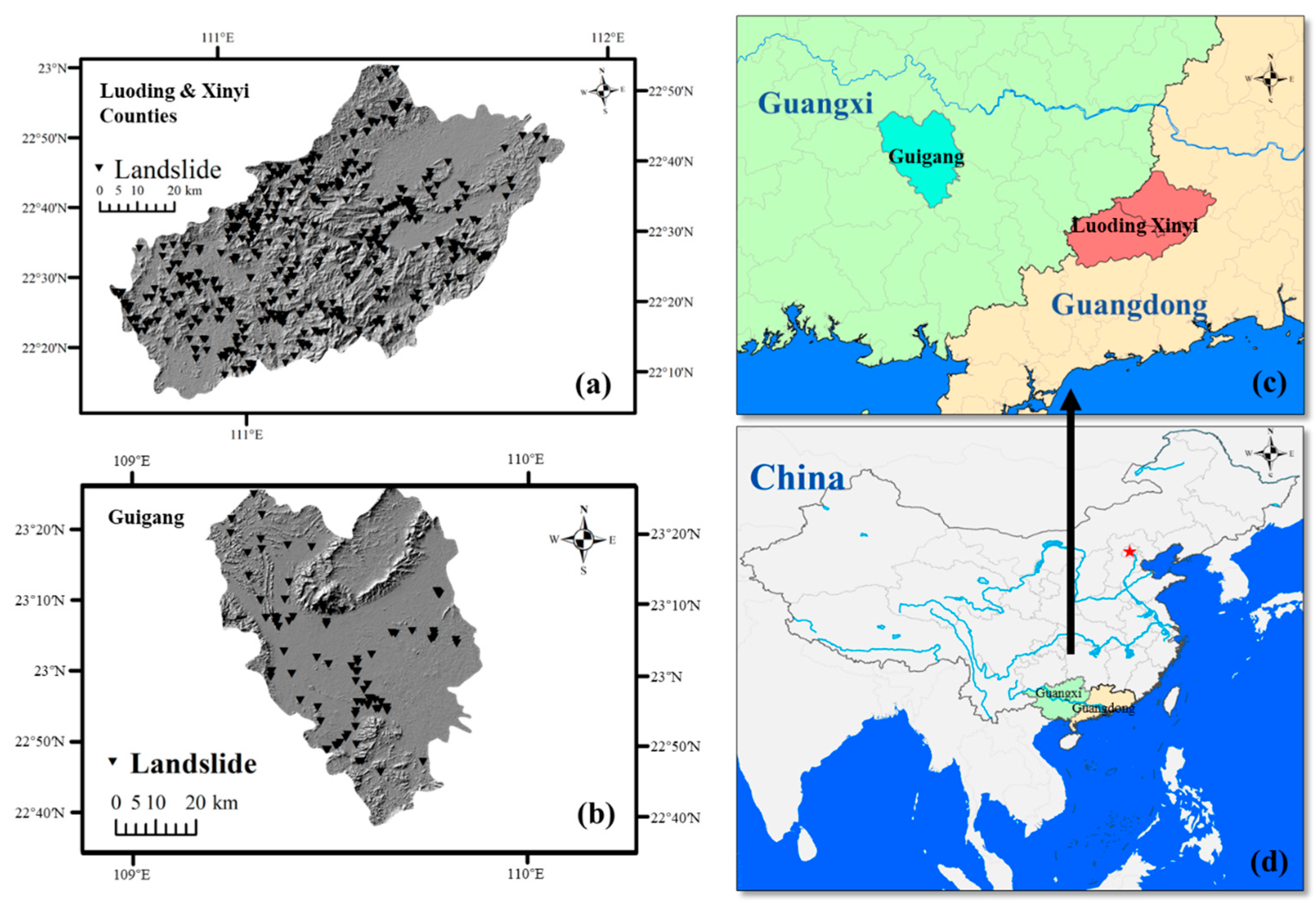
Figure 1. Landslide inventory maps of first two study areas in China. (a) the first one across Luoding County and Xinyi County (LX) of Guangdong Province, (b) the second one in Guigang County (GG) of Guangxi Province, (c) the locations of the study areas in Guangdong Province and Guangxi Province, (d) the locations of the two provinces in China.
Land 12 00525 g001
Figure 2. Thematic maps of the Luoding and Xinyi counties: (a) altitude (meter), (b) aspect, (c) distance to faults (meter), (d) distance to rivers (meter), (e) distance to roads (meter), (f) land use, (g) lithology, (h) normalized difference vegetation index (NDVI), (i) plan curvature, (j) profile curvature, (k) rainfall (mm/month), (l) surface roughness (so-called standard deviation of the slope—SDS), (m) slope (°), (n) topographic wetness index (TWI).
Land 12 00525 g002
Figure 3. Thematic maps of Guigang Province: (a) altitude (meter), (b) aspect, (c) distance to faults (meter), (d) distance to rivers (meter), (e) distance to roads (meter), (f) land use, (g) lithology, (h) normalized difference vegetation index (NDVI), (i) plan curvature, (j) profile curvature, (k) rainfall (mm/month), (l) surface roughness (so-called standard deviation of the slope, SDS), (m) slope (°), (n) topographic wetness index (TWI).
Land 12 00525 g003
Figure 4. Overview workflow in this study.
Land 12 00525 g004
Figure 5. Overview of a VAEGAN.
Land 12 00525 g005
Figure 6. The illustration map of generating the data with attributes by a VAE.
Land 12 00525 g006
Figure 7. Transfer learning and transfer learning with attributes.
Land 12 00525 g007
Figure 8. Importance of landslide-influencing factors, based on (a) LX and (b) GG.
Land 12 00525 g008
Figure 9. Selected CNN model by Bayesian optimization.
Land 12 00525 g009
Figure 10. LSMs generated by CNNs. (a) LX and (b) GG. SL = supervised learning.
Land 12 00525 g010
Figure 11. (a) AUROC curves and (b) training efficiency on validation set of SL, TL and TLA. The symbol “LX→GG” represents the fact that the LSP model is pretrained by the data set of LX and then fine-tuned by the data set of GG, and the L X ¯ represent the reconstructed data that contains the attributes of the data set in LX and the data set in target domain (e.g., GG).
Land 12 00525 g011
Figure 12. AUROC curves on testing data set of (a) CNN, (b) GRU and (c) BiLSTM. The contents in the bracket, such as (CNN, GRU), represent that the decoder of VAEGAN is CNN and that of LSM models is GRU, respectively.
Land 12 00525 g012
Figure 13. Training efficiency of (a) CNN, (b) GRU and (c) BiLSTM.
Land 12 00525 g013
Figure 14. LSMs of GG using (ac) SL, (df) TL and (go) TLA.
Land 12 00525 g014
Figure 15. FR values of LSMs (GG) in high and very high susceptibility zones: (a) comparison in LSP models, (b) comparison in transferability of CNN, (c) comparison in transferability of GRU, (d) comparison in transferability of BiLSTM.
Land 12 00525 g015
Figure 16. Landslide inventory maps of Zigui County.
Land 12 00525 g016
Figure 17. AUROC curves on testing data set of (a) CNN, (b) GRU, (c) BiLSTM.
Land 12 00525 g017
Figure 18. Training efficiency of (a) CNN, (b) GRU, (c) BiLSTM.
Land 12 00525 g018
Figure 19. FR values of LSMs (ZG) in high and very high susceptibility zones: (a) comparison in LSP model, (b) comparison in transferability of CNN, (c) comparison in transferability of GRU and (d) comparison in transferability of BiLSTM.
Land 12 00525 g019
Figure 20. The mean value of evaluators in different numbers of samples participating in the study area (GG, target area; LX, source area).
Land 12 00525 g020
Figure 21. The mean value of evaluators in different numbers of samples participating in the study area (ZG, target area; LX, source area).
Land 12 00525 g021
Table 1. The information about landslide-influencing factors used in this study [28].
#CategoryFactorsReason for SelectionData Source
1TopographyAltitudeSlope is closely related to the local altitude, so altitude is one of the factors that influence landslides [29].The digital elevation model (DEM) with a 30 m resolution of the study area can be downloaded from http://www.gscloud.cn/home (accessed on 23 June 2022).
2 Slope angleThis directly affects slope stability and has been widely used in landslide sensitivity analysis [9].DEM derivatives.
3 AspectThis is related to the landslides in that slopes in different orientations are differently affected by precipitation and solar radiation [30].DEM derivatives.
4 Plan curvatureThis reflects the rate of change of the aspect along the contour and thus can affect the flow of water across a surface [31].DEM derivatives.
5 Profile curvatureThis influences the acceleration and deceleration of flow through slope; thus, some valuable information about erosion and deposition is provided [32].DEM derivatives.
6 SDSThis is an index reflecting the degree of surface fluctuation and erosion intensity [33]. S D S = 1 / cos ( s l o p e ) .
7 TWITWI describes the topographic properties of hydrological processes in that both slope and local upslope contribution areas are considered [34]. T W I = L n ( S C A / tan β ) , where SCA is the specific catchment area ( m 2 / m ) and β is the slope angle (degree) of the position.
8EnvironmentalLand useLand use is a key factor in landslides and has an important influence on the stability of slopes thanks to vegetation cover [35].Land-use data are from a study in 2015 [36].
9 RainfallThis is a key landslide-inducing factor in that it can affect the shear strength of the slope [37].The rainfall (mm/month) raster data in the study area were obtained by using the inverse-distance weighting interpolation method [38] on rain stations (http://data.cma.cn/, accessed on 5 January 2022) in the vicinity of the study area.
10 NDVIThis reflects the greenness of an area and may alter the distribution of soil and hydrological processes on slopes [39].The NDVI data were obtained from the MOD13Q1 product, which were downloaded from https://search.earthdata.nasa.gov/search (accessed on 3 July 2022) and processed by the MODIS projection tool [40]. Furthermore, in order to minimize potential atmospheric effects, the NDVI data used in the paper are the average value of the entire year of 2015.
11 Distance to riversRivers affect slope stability in that they can cut and erode banks, and these actions reshape and sculpt the landscape. In addition, fluctuations in the water level greatly affect the groundwater level of the slope [29].The data come from the National Geomatics Center of China (http://www.ngcc.cn/ngcc/ (accessed on 20 May 2022), and the Euclidean distance tool of ArcGIS is used to obtain the river distance in the study area.
12 Distance to roadsThis is considered to be one of the most important human factors affecting the occurrence of landslides [7].The method of obtaining the road distance raster data is the same that for obtaining the river distance.
13GeologicalLithologyThe mechanical and hydrological properties of rock masses (such as permeability and friction angle) differ between lithological units, so this factor can greatly affect slope stability [37].Geological maps of the study area were obtained from the National 1:200,000 Digital Geological Map (Public Edition) of China [41]. The description of the lithological formations in the study areas are shown in Table A2 of Appendix A.
14 Distance to faultsThis has an important influence on the distribution and scale of landslides in the study area [30].The data on the locations of faults in the study area were obtained from the National 1:200,000 Digital Geological Map (Public Edition) Spatial Database of China [41], and The Euclidean distance tool of ArcGIS was used to obtain the fault distance in the study area.
Table 2. The best-selected parameters of CNNs.
GroupParametersSearch SpaceBest Value
CNN architectureConvolution kernel number [1, 5]3
Max pool layer number [0, 5]0
CNN hyperparametersConvolution kernel size [1, 6]6, 1, 4
Convolution kernel channel [8, 16]16, 32, 64
Max pool size [0, 5]0
Dropout rate [0.1, 0.7]0.2249
Training optionsInitial learning rate [0.001, 1]0.0059
Learn rate schedulepiecewise decay, constantpiecewise decay
Learn rate drop period [1, 10]2
Learn rate drop factor [0.1 0.9]0.1462
minibatch size [6, 30]30
Table 3. LSM model performance comparison in LX and GG (supervised learning).
Study AreaModelEvaluators
AUROCAccuracyPrecisionRecallF1-ScoreMean
LXCNN0.8630.7710.7880.7610.7750.792
GG0.8020.7350.8330.7140.7690.771
Note: Bold font is the best case.
Table 4. Transferring ability comparison of different methods (LX to GG).
TrainingTestingExperiment Model
CNN
LXLXA (SL)0.771
LX & GGGGB (TL)0.772
L X ¯ & GGC (CNN-VAEGAN)0.844
Note: the scores in the table represent the mean value of evaluators; boldface indicates the best case.
Table 5. LSM models performance comparison in LX and GG (supervised learning).
Study AreaModelEvaluators
AUROCAccuracyPrecisionRecallF1-ScoreMean
LXCNN0.8630.7710.7880.7610.7750.792
GRU0.8360.7710.7560.6940.7240.756
BiLSTM0.8320.7530.7090.8590.7770.786
GGCNN0.8020.7350.8330.7140.7690.771
GRU0.7840.5590.8000.3810.5160.608
BiLSTM0.7140.7060.7390.8100.7730.748
Note: Boldface indicates the best case.
Table 6. Comparison of the transferability of different models (LX to GG).
TrainingTestingExperimentModels
CNN GRUBiLSTM
GGGGA (SL)0.7710.6080.748
LX & GGB (TL)0.7720.7100.770
L X ¯ & GGC (CNN-VAEGAN)0.8440.6980.767
L X ¯ & GGD (GRU-VAEGAN)0.7830.6890.746
L X ¯ & GGE (BiLSTM-VAEGAN)0.7930.7080.783
Note: the scores in the table represent the mean value of evaluators; boldface indicates the best case.
Table 7. LSM models performance comparison in ZG (supervised learning).
Study AreaModelEvaluators
AUROCAccuracyPrecisionRecallF1-ScoreMean
ZGCNN0.8000.7470.7040.8520.7710.775
GRU0.7290.6910.6630.7770.7160.715
BiLSTM0.7540.7100.6890.7650.7250.729
Note: Boldface indicates the best case.
Table 8. Comparison of transferability of different models (LX to ZG).
TrainingTestingExperimentModels
CNN GRUBiLSTM
ZGZGA (Supervised Learning)0.7750.7150.729
LX & ZGB (TL)0.7530.7160.734
L X ¯ & ZGC (CNN-VAEGAN)0.8180.7300.731
L X ¯ & ZGD (GRU-VAEGAN)0.7940.7080.674
L X ¯ & ZGE (BiLSTM-VAEGAN)0.8040.7350.741
Note: the scores in the table represent the mean value of evaluators; boldface indicates the best case.
Disclaimer/Publisher’s Note: The statements, opinions and data contained in all publications are solely those of the individual author(s) and contributor(s) and not of MDPI and/or the editor(s). MDPI and/or the editor(s) disclaim responsibility for any injury to people or property resulting from any ideas, methods, instructions or products referred to in the content.