1. Introduction
1.1. Informal Green Space—A Retrofit for Urban Green Space
Based on scientific studies, green areas in the living environment positively affect one’s mood, helping to reduce stress and improve work productivity [
1,
2,
3,
4]. Urban green spaces (UGSs) provide a range of ecosystem services that can help resolve many problems of urbanization, such as urban heat islands, noise pollution, and air pollution [
5,
6,
7,
8], and offer physical and mental benefits for human health [
9,
10]. Although the UGSs could be used to define any vegetation within the urban area, the government and the city’s management staff usually recognize the formal green spaces (FGSs), such as urban parks, forest parks, and garden parks, as the spaces designed for public greenery services. However, with the increase in population residing in urban areas [
11], there is a dire need for contact with the natural environment due to the lack of FGSs. In the past decade, insufficient green areas and their unfair distribution to urban residents have been significant issues that have attracted remarkable attention [
12,
13,
14]. Large cities have a scarcity of FGSs, and the data show that big cities’ global average standard for UGS per capita is generally markedly lower than the recommended standard of 10 m
2/person [
15]. For example, the average UGS per capita is 4.5 m
2 in Tehran, Iran [
16]; 4 m
2 UGS per person [
17] in Kyoto, Japan; and only nearly 2 m
2 in Ho Chi Minh City (HCMC) and Hanoi, Vietnam [
18]. To account for this situation, cities increasingly aim to supplement and expand the green spaces in urban areas. Nevertheless, in recent years, many FGS projects have been postponed or cancelled due to the economic recession, financial constraints, the urgent need for other social development projects, and the heavy economic consequences of the pandemic. These observations have inspired research into the different types of vegetation in urban areas that can be used to supplement FGSs [
17,
19].
Recently, formerly neglected areas, such as vacant lots and wastelands, and urban agriculture have garnered increasing attention [
20,
21,
22,
23]. As the critical difference from FGSs, governing institutions have yet to officially recognize these spaces designated for forestry, gardening, recreation, and environmental protection. Any land used for recreational purposes is deemed informal and transitional [
24]. These areas are collectively called informal green spaces (IGSs) to maintain academic consistency and coherence. They are explicitly defined as socio-ecological entities instead of being solely cultural or biological. They can be found in developed [
19,
25] and developing nations and can be used to benefit the community while maintaining the budget for urban greenery preservation. The research has also pointed out that the management of IGSs with volunteer participation can improve the aesthetics of urban landscapes while meeting the needs of the residents [
17]. Studies have been conducted on residents’ perceptions and the distribution of UGSs and IGSs in Ichikawa City, highlighting the potential of IGSs as complements to FGSs and their role in alleviating the spatial and financial burden placed on the government [
19,
26]. Several studies about IGSs in developing countries such as Afghanistan and Morocco have also been conducted [
15,
27]. However, due to IGSs being smaller than large-scale urban parks and having irregular spatial continuations, they have been overlooked by governments because of the challenges in detecting and analyzing their distribution and because they are rarely widely used.
1.2. A New Method to Survey Informal Green Spaces
The traditional survey methods for green infrastructure use remote sensing imaging techniques to map and quantify green spaces in cities due to their many advantages, such as the ample area coverage, synoptic view, and repeatability, as discussed in previous studies [
28,
29,
30]. Nevertheless, small IGSs under large tree canopies are usually miscalculated or overlooked in the top-down view or can be archived with high-quality and expensive remote sensing products. To tackle this issue, Ta et al. [
31] proposed a survey method using Google Street View (GSV) combined with machine learning to automatically survey IGSs in large areas. The method takes advantage of new technology while reducing the drawbacks of the traditional survey methods using airborne (plane or satellite) images.
GSV, which allows users to freely change their field of view through point positioning along several streets in the United States, was first introduced in 2007 and became popular worldwide one year later, in 2008, after applying a computer algorithm that could blur people’s faces to protect their personal information. It was integrated into many platforms, such as Google Earth, Google Maps, and the Google Maps applications on both Android and Apple smartphones. Google encourages users to directly contribute their panorama photos to the GSV database to enrich its data. This feature and the development of high-quality cameras have allowed GSV to cover 16 million kilometers (according to Google in 2022) across 102 countries. As a result, numerous studies have considered GSV data as trustworthy sources to conduct surveys on various entities, ranging from neighborhood environments [
32] to street greenery [
33,
34,
35] and even solar radiation within street canyons [
36].
Besides GSV, machine learning was also introduced by Ta et al. as a tool to analyze and detect IGSs in complex scenarios instead of human labor [
31]. Machine learning, in which computers learn from past experiences (i.e., input data) and make predictions on par with the human brain’s abilities, has undergone extensive development since its introduction in 1959 by Arthur Samuel. This advanced method can classify images into components, such as humans, trees, skies, and cars, based on differences in pixel numbering, and has recently been used by many researchers due to its efficiency for urban street scenes [
37], the green view index [
38], and socioeconomic characteristics [
39]. Machine learning can significantly reduce the workload while ensuring high-quality performance and project progress. By creating a trustworthy model for computer learning, AI can be used to detect small objects (such as IGSs) in pictures more efficiently than a human could because of the AI tool can analyze pixels. Combining these two new technologies, the proposed method could be operated by any user and in any place around the world, so major cities around the world could use it and integrate IGSs into their urban green space systems as a retrofit for formal green spaces.
1.3. The Purpose of the Study
Nowadays, many governments worldwide aim to archive equal green spaces for every capita in major cities. That purpose hardly reaches only FGS, while IGS promise a bright potential as a supplement material for FGS in order to increase total UGS. Hence, to adapt to this desire, Ta et al. proposed a survey method to survey IGSs beneficial to integrate IGSs into the UGS system. One of the limits of the previous research on the new IGS survey method in 2021 was that it only proposed a theoretical base and mentioned the possibility of using it without practice and a comparison to evaluate its effectiveness [
31].
Therefore, this study focused mainly on IGSs and had three aims. The first aim was putting the IGS survey method theory, using machine learning to automatically detect IGSs in GSV photos, into practice by using the same study area, which was Ichikawa, Japan. Secondly, this study used ArcGIS to create a distribution map and density heatmap of Ichikawa to test the method’s effectiveness by comparing the results with the field survey results previously obtained from northern Ichikawa [
26]. Finally, the aim was to apply the method in a new study area, HCMC, Vietnam, to evaluate its ability to be used worldwide. Although the study was only conducted in two cities in Japan and Vietnam, the research results could demonstrate that this method could be helpful as a low-cost and supportive tool for urban environmental analyses.
This paper first introduces the study sites, Ichikawa city and HCMC, with their similar attributes before explaining the survey method and the modifications we made to further improve the method’s efficiency when applied. The results of training the model’s accuracy and the distribution map of Ichikawa city is presented, followed by a comparison with the previous research map. The two IGS maps of HCMC are explained detailed next before conducting a more comprehensive discussion about the content of this research.
2. Materials and Methodology
2.1. Study Sites
2.1.1. Ichikawa, Japan
Ichikawa City, located in northwest Chiba Prefecture, Japan, was selected as a study site (
Figure 1), since two field studies about IGSs were previously conducted here [
19,
26]. Ichikawa City covers an area of 57.45 km
2, with a population of approximately 485,852 (as recorded in 2020). Although this city has experienced high rates of population mitigation three times, the government did not organize its urban infrastructure. In addition, owing to its proximity to Tokyo, the influence of outer Tokyo, land re-adjustment processes, and railway construction in this city has been significantly strengthened. Currently, 70% of Ichikawa is an urbanized area, including accommodation, industrial, and commerce districts, while nearly 30% is an urbanization control area used to contain urban sprawl. As of 2016, the city provided 3.43 m
2 of green space per capita, despite the city government’s efforts to improve residents’ quality of life through several city plans since 2000 [
40,
41]. The opportunity to use green spaces also differs for each person relative to the requirement of the Urban Park Act of Japan, which requires a minimum of 10 m
2 of urban parks per capita. The city provides nearly 7 km
2 of green facilities for general greenery, including 3.45 km
2 of urban parks, 2.27 km
2 of public green open spaces, and 1.21 km
2 of private facility green spaces. Thus, the greenspace area per capita is only 7.28 m
2, far from meeting the above standard. The city is divided into various land use patterns: >60% comprises residential, trade, and industrial districts, and 30% comprises urbanization control areas with agricultural districts and forests. All industrial districts are located in the southern region, while the northern area includes all agricultural districts and forests and most urbanization control areas.
2.1.2. Tan Binh and Phu Nhuan Districts in Ho Chi Minh, Vietnam
Tan Binh and Phu Nhuan (TBPN) districts, located in the central area of HCMC, Vietnam, were selected as the second study sites (
Figure 2). The TBPN districts have an area of approximately 27.43 km
2, with a population of roughly 653,000 in 2021.
This study included these districts due to their shared characteristics with Ichikawa, Japan. First, the TBPN districts have the same influence as the central districts, similar to Tokyo’s effect on Ichikawa. These two districts were formally established in 1975 and are bordered by central districts, such as districts 1, 3, and 10. These districts also have industrial areas, mainly in the Tan Binh district, as well as a vital railroad leading to other regions. Accordingly, the infrastructure in the TBPN districts is severely fragmented, making it difficult for the government to provide adequate and equitable green spaces for the citizens, with plans until 2030 to designate nearly 3% of the total area for green infrastructure. UGSs in this area and the whole city have markedly changed, as the city is considered a developing city. Therefore, the planning and use of infrastructure regularly require a master city plan and individual actions. Second, cutting down trees in the central districts to obtain more space for city development increases the residents’ demand for green spaces. The urban areas only contain 54 km
2 of greenspace, equal to 1% of the total greenspace of the city. Therefore, the average green coverage of the urban zones remains as low as 1.95 m
2 per person. In some cases, this area decreases to 0.69 m
2 per person. According to the Department of Transport, the statistical analysis of HCMC revealed a rate of 13.7 m
2 per citizen [
42]. TBPN contains two of the ten large parks in HCMC, Gia Dinh Park, Hoang Van Thu Park, and some neighborhood parks. Hence, the number of people moving to TBPN for these UGSs has markedly increased in recent years. In the past two decades (2000–2020), the population of the TBPN districts has increased by more than 1.5-fold, and almost all residents have migrated from rural areas to TBPN in search of work. To date, no study has focused on exploring the use of IGSs as a retrofitting solution for this issue in Vietnam.
2.2. Google Street View Panorama Collection and Cube Map Conversion
In this study, all images collected by the Street View Download 360 program in Ichikawa and HCMC were pre-processed via cube map conversion to prepare the data for the next stage. The distance between the interval points was selected as 78 m, similar to the proposed 2020 study [
31], according to the size of the study sites. As the previous research indicates, the popular distances are 20 m [
33], 50 m [
34,
43], and 100 m [
44,
45]. A study site with an area <1000 m
2 generally uses a distance range of 20–50 m, whereas sites >400 km
2 use a distance of 100 m. Considering the actual situation, for a small distance, the field of view for every three consecutive photos will overlap, resulting in overcounting of the number of spots that have IGSs; large distances can leave a gap between two spots, resulting in reduced accuracy and effectiveness for this method. A distance of 78 m can considerably avoid the overlap issue and leaves an acceptable gap between the two spots. A network of points with 78 m intervals along the path was created in the study area, and the GSV photos were downloaded from these points. The downloaded photos are the latest uploads based on date, with the dates ranging from 2016 for alleys or small streets to 2020 for large areas with easy car movement. The program automatically eliminated almost all photos taken indoors. In addition, the panoramic images were in an equirectangular format, with objects near the side edges being strongly bent (
Figure 3). Therefore, the cube map conversion program was used to preserve and prevent distortions during the flattening process.
The cube map conversion process provides a method to reduce the distortion of the flattening process. The cubic format, or cube map, creates a cubic square surrounding the spherical panoramas and reflects the image onto the nearest face of the cube. Hence, after reflection on all six given faces (left, front, right, back, top, and bottom) with 90° field of view cameras (
Figure 4), the cubic square is displayed as an unfolded cube.
Using this method, all photo data from the Ichikawa and TBPN districts were converted using a Python program.
2.3. Setup Training Model and Semantic Segmentation
DeepLabV3+ was used to classify and detect green areas in the GSV images. In 2018 this network was introduced, and void convolution was used to control the resolution of the output feature map; therefore, striking a balance between the exactness and operation time [
37]. Using a set of sample pictures, this program was first trained to recognize, separate, and label IGSs in panoramic pictures. To serve as data for the model training process (i.e., sample pictures), 1000 photos were selected from Ichikawa’s dataset downloaded in the step above, under the condition that each possess one or more IGSs in different contexts, such as near forests, parks, cityscapes, and residential areas; these can be recognized using a regular view (i.e., viewed on screen without magnification). Subsequently, the IGSs were labelled manually by a graduate student who studied the landscape using the Labelme program (
Figure 5). A new model was generated through a training process using labelled images as the input data for machine learning. An evaluation program was run to check the model’s accuracy before being imported into DeepLab V3+ for the next step.
In this step, Deeplab V3+ used the provided model to automatically recognize and mark all IGSs in the cube map photos. This program processed all images in both research areas. Next, the photos containing IGSs were selected and copied with their coordinates.
2.4. Creating IGS Distribution and Density Maps
In this step, the photos containing IGSs obtained from the previous step were imported into ArcGIS to create distribution maps of IGSs in Ichikawa and the TBPN. The IGS distribution maps were established with more detailed documentation. A heat map displaying the density levels of IGSs in each area was also generated from the distribution map. To evaluate the efficiency of this method, the final map of Ichikawa was compared to data on the IGSs’ distribution recorded in the northern part of Ichikawa in 2020 [
26].
The following process was conducted to archive the final result (
Figure 6):
3. Results
3.1. Images Downloaded and Training Model Accuracy
A total of 24,553 photos were downloaded in both study areas, comprising 15,429 GSV images of Ichikawa and 9124 GSV images of the TBPN districts (
Table 1). In Ichikawa, the photos were used to assess the theoretical basis and compare it with the previous research [
19,
26] to improve our understanding of the IGSs. The images collected were of considerable high quality (in terms of photo resolution), with more than 80% of them measuring 2048 × 1024 pixels. In comparison, approximately 30% of the pictures of TBPN could be considered high-quality images. Given the quality of the images, the accuracy of the following steps was also affected, since the program could not clearly determine the shapes of the subjects in the picture, especially subjects near two edges.
The process was modified based on the application to improve the accuracy and generate detailed results. Compared with the method proposed [
31], this study included the cube map conversion before the training model and segmentation steps. As a result, the bending effect along the edges of the photos was reduce drastically. DeepLab V3+, which used a model created with 1000 photos, gave an accuracy rate of approximately 0.65 for the designated samples. This result indicated that the new model’s accuracy had a ~65% match with the masked (labelled) image given in the training process (
Figure 7). This means the program can detect IGSs in the photos, although in some cases, it will mistake objects of a similar size (small), shape (oval, rectangular, triangle), or color (light green to dark green) as IGSs, and it may overpass the IGSs in some photos.
Furthermore, the density heatmap was also generated to visualize the density of the IGSs, since the effect of the IGSs has a tight relationship with their spatial distribution and affects the group of residents. In addition, the HCMC was used to test the efficiency of the novel model in areas outside Japan. This map could be used as the base information for field research in the future.
3.2. Ichikawa, Japan
Based on the distribution map of north Ichikawa (i.e.,
Figure 8a) that was generated using our novel method, the IGSs were densely distributed into two-thirds of the area of northern Ichikawa City. Furthermore, high densities of IGSs were identified in the northeastern and northwestern parts of northern Ichikawa. A site to the south with few or no IGSs was also clearly observed.
A distribution map from a study on the distribution of IGSs in northern Ichikawa in 2020 [
26] generated from field survey data was used as a comparison. The map was obtained from an assessment of the typology of and perceptions of local residents about IGSs. A grid net of 500 m × 500 m was established with sample sites of approximately 2500 m
2 at each intersection along northern Ichikawa, and the mail-back kit was distributed in those sample sites. Each mail-back kit included a questionnaire survey and a brief explanation (with pictures to visually identify) about IGSs. A total of 120 sites were surveyed, and data on the land use, morphology, and vegetation were collected (
Figure 8b). The IGSs were found to cluster around two main areas, namely the east and west of northern Ichikawa, but were scattered in other areas.
In order to maintain unity with the previous research by Min et al. [
26], this study used the same criteria for identifying IGSs to create the training model created by a graduate student studying landscape architecture. As a result, all IGSs determined by the program were detected as having the exact definition of the field survey.
The two maps show several similar patterns in the distribution of the IGSs. These patterns could be seen at high density in the middle and lower parts of the east side of northern Ichikawa, with IGS percentages ranging from 20.1% to 100%. The center and south sides of this city’s northern part present many areas with little or no IGSs in both maps. However, the difference between them is shown clearly on the west side of this region. The map generated by the new method indicates dense IGSs here on the top part of the west side, which are hardly seen on the other map. The middle part of this region in the previous study showed two sample sites with 20% to 100% IGS percentages, but IGSs are scattered in the new maps.
Nevertheless, this new method can produce an IGS distribution map with more detailed documentation than the previously used methods while reducing the workload for the researchers.
For further comparison, this new method was found to collect more detailed data, with 3029 spots (each spot represents one photo) and could detect IGSs in 15,429 images of Ichikawa (
Table 1). This result showed the distribution of the IGSs south of Ichikawa; such data were not obtained in the previous research. The IGSs in this area were significantly fewer than those in northern Ichikawa City and tended to be located along the Edo River (
Figure 9a). A heatmap was created using ArcGIS to determine the density of IGSs in the city. The IGS density was calculated using the number of IGSs in 1 km
2 and was displayed through a color range of 10 grades, from light to dark purple. Here, the most vivid color indicates a dense area with 150–167 IGSs/km
2, while the lightest color indicates 1–16 IGSs/km
2 (
Figure 9b). Therefore, the hot spots of IGSs can be observed in this heatmap and are located in three places as described above: the top northwest, the northeast side, and along the Edo River in the south.
3.3. Tan Binh and Phu Nhuan Districts in HCMC, Vietnam
In the TBPN districts of HCMC, 204 spots were detected to have IGSs from a total of 9124 photos downloaded from the Google server (
Table 1). The distribution map of the IGSs revealed the average density, i.e., 9.9–14.9 IGSs per km
2, with primary concentrations in the eastern, southern, and northwestern parts. Of note, the central and northern parts did not have any IGSs, except for a few spots at the surrounding edges (
Figure 10a). This decreased rate was caused by several factors, including the many low-resolution, mislocated, nighttime, and indoor photos, making it difficult for the program to accurately recognize the objects in complex scenes. As depicted in the map in
Figure 8a, IGSs can be detected in all districts, except a large area in the north of Tan Binh district, at the Tan Son Nhat International Airport, which restricts people’s access. Another notable characteristic of the distribution of IGSs in TBPN is the straight line of IGSs east of the maps, which belongs to the Phu Nhuan district. IGSs exist on the side of the railway named the “railroad verge” [
17,
19]. The heatmap generated from the data derived using the same method as the Ichikawa case provides a clear view of the density of IGSs in the TBPN district. However, Ichikawa has density values ranging from 1 to 167 IGSs per km
2, while the TBPN district has IGS density values ranging from 1 to 25 IGSs per km
2, nearly seven times less than Ichikawa (
Figure 10b).
The same display method applies to this area: the dark purple indicates 22–25 IGSs/km
2, while the lightest pink indicates 1–2 IGSs/km
2. Thus, the hotspots are two areas south of the Tan Binh district (
Figure 11a,b) and the railway on the Phu Nhuan district’s east side (
Figure 12a,b). In addition, there are four hotspots with 10–12 IGSs/km
2 areas encircling the airport and two at the boundary of the Phu Nhuan district with other districts.
4. Discussion
IGSs are generally small areas that are widely dispersed; therefore, they are easily detected through detailed field surveys. However, mapping the IGS distribution in this way requires considerable time and effort. It is challenging to apply remote sensing methods using airborne technologies or satellites to survey IGSs, as it is difficult to separate and detect IGSs owing to their small size. In addition, most remote sensing devices remain inaccessible to non-experts, such as urban managers and planners, as detailed remote sensing products are generally expensive. Furthermore, the distinguishing characteristics of the profile view on the ground provides detailed information. It takes a long time to analyze such images, while the overhead view from remotely sensed images is quick but cannot fully reflect a pedestrian’s perspective (
Figure 13). Of note, studies have been conducted on this issue [
48,
49]. The issues above can obstruct municipal forest managers from planning and using IGSs to retrofit FGSs.
Street-level images, particularly GSV images, resemble the view of pedestrians, thereby providing a human-centric method to map the spatial distribution of IGSs. Such images have been used and have led to good results in studies of greenery classification in urban streetscapes based on analyses of green pixels in images [
48,
50], as well as studies on the distribution of small objects such as forest pests via the identification of distinctive nests [
51].
In addition, GSV is a convenient geospatial platform that is easy to use anywhere, providing ground-based panoramic photographs captured along streets, both online and through Google Earth. GSV only requires a simple interface that anyone can use with minimal effort (
Figure 14). Such simplicity addresses the limitations of the previous research and confirms GSV’s ability to produce the same results as field surveys while reducing the costs and safety risks [
52].
Despite the advantage of GSV’s perspective, it challenges the operator due to the immense quantity of photos, which number more than 50,000 in some cases. Applying a machine learning technique, such as semantic segmentation, effectively reduces the workload while ensuring the performance. Although the accuracy of this research could be low, it is also evident that this new method could operate well in both places—the city that the sample photos came from and a new city in a different country.
By applying the new method using GSV and semantic segmentation, robust surveys that will yield detailed results can be conducted while addressing the limitations that impede field surveys owing to the extensive study area and high research costs. The maps produced through this method gave more detail than the traditional ones. All of the photos with geotags attached to them from the beginning were imported into ArcGIS and pinned to the appropriate locations automatically. As a result, the maps were created with great detail while requiring less effort from the surveyors. We assessed the possibility of using IGSs to increase the total green space areas in dense urban areas without weighting the city’s economies, allowing every citizen to have an equal chance of experiencing green space.
This study also involved a practice check on the proposed method against previous research and consolidated a framework for future research to assess green spaces in dense urban areas.
There are some limitations in this research. The images downloaded from GSV have a wide range of resolutions; thus, the program made several mistakes when detecting IGSs in complicated contexts, mainly when the images contained many people or formal green spaces, such as parks. This problem could be resolved with the development of recording technology, which could provide more detailed photos. Even though limitations exist, this study proves that it is possible to continue studying and developing the method using GSV and machine learning and to apply it in more practical cases.
The small sample training set, which comprised only 1000 photos and was taken only from Ichikawa’s photo set, was another issue, ultimately resulting in a relatively low accuracy rate (>60%) not only for Ichikawa but also for the TBPN districts. For future research, a more extensive image database should be developed for training models, including 10,000–30,000 labelled photos collected from different places. Further, a closer interval network that could be used to obtain the GSV photos should be derived.
5. Conclusions
Studying the IGS distributions in HCMC, Vietnam, and Ichikawa, Japan, offers an excellent opportunity to improve our understanding of the situation regarding IGSs. Herein, a method was developed to create IGS maps by combining Google Street View (GSV) images and machine learning methods. This method has proven its effectiveness by taking advantage of the pedestrian view level to detect small and covered subjects from a top-down perspective. Additionally, after developing the model stage, this method can be operated easily by non-professional users. As a result, two IGS distribution maps were established in Chiba and HCMC. The maps in HCMC and the southern part of Ichikawa City were the first set, and for the northern part of Ichikawa we added new material in this study.
A total of 24,553 GSV images were downloaded from Street View Download 360 using a network of interval points along the road to detect the IGSs. The novel model proposed in this study for DeepLab V3+ was constructed from 1000 manually labelled pictures to recognize and mark IGSs in the GSV data. The IGS distribution maps and density heatmaps were produced from the output data from DeepLab V3+ using the ArcGIS software. This method produced results consistent with the previous fieldwork, required less effort, and could be performed automatically in any country. Therefore, this method can reduce the human risk and research costs compared with traditional field survey methods.
Based on the results of this study, the number of IGSs in Ichikawa, which is a city in a developed country, is significantly higher than that in the TBPN districts in HCMC, which are located in a developing country, owing to the large number of consistently high-quality GSV images that allow Deeplab V3+ to detect IGSs on-scene easily. Besides testing the effectiveness of the survey method, we proposed a hypothesis that developed countries have more IGSs than developing countries, as the master plans and urban planning are stable and are taken seriously for environmental protection. In contrast, in locations within developing countries, such as HCMC, there are vacant land spaces or voids with high potential for conversion to IGSs. Urban plans often change rapidly according to the speed of urbanization and socioeconomic development. Additionally, people take advantage of and encroach on public spaces for personal purposes [
53]. This result also shows that the green ratio of the cities can be assessed using this method based on the total area of public green spaces and IGSs instead of calculating the percentage of public green space as previously performed. On the other hand, the sum of IGSs and public green spaces may indicate a high level of global green space.
Although this method can be used globally, depending mainly on the quality of the GSV photos, it tends to work more efficiently in developed countries where GSV photos are of higher resolution and have higher geotagging accuracy than in developing countries. The GSV network is still lacking in some countries, such as China, Russia, and West Asian countries. It also cannot be used in situations requiring the newest data for specific areas because of the long GSV photo update intervals. Another limitation is the small image database used for the training models. Based on this study, only 1000 images in Ichikawa’s set of images provided relatively low accuracy (>60%). A more extensive image database should be developed for training models (for example, using approximately 10,000–30,000 labelled images) and in locations within a close-distance network.
Author Contributions
D.T.T. conceived, designed, and conducted the survey; utilized the program; and wrote the initial draft; K.F. provided support in terms of the research design, summarization, and revision of the article. D.T.T. finalized the paper. All authors have read and agreed to the published version of the manuscript.
Funding
This study was funded by the Landscape Planning Laboratory of the Graduate School of Horticulture, Chiba University, Matsudo.
Institutional Review Board Statement
Not applicable.
Informed Consent Statement
Not applicable.
Data Availability Statement
Not applicable.
Acknowledgments
The authors would like to thank their friends and supervisors for their technical support and coding advice throughout this research.
Conflicts of Interest
The authors declare no conflict of interest. The funding organizations had no role in the study’s design; in the writing of the manuscript; in the decision to publish the results; or in the collection, analysis, or interpretation of the data.
References
- McFarland, A.L. The Relationship between the Use of Green Spaces and Public Gardens in the Work Place on Mental Well-being, Quality of Life, and Job Satisfaction for Employees and Volunteers. HortTechnology 2017, 27, 187–198. [Google Scholar] [CrossRef]
- WHO Regional Office for Europe. Urban Green Spaces: A Brief for Action; WHO Regional Office for Europe: Copenhagen, Denmark, 2017; pp. 1–24. [Google Scholar]
- Ma, B.; Zhou, T.; Lei, S.; Wen, Y.; Htun, T.T. Effects of urban green spaces on residents’ well-being. Environ. Dev. Sustain. 2019, 21, 2793–2809. [Google Scholar] [CrossRef]
- Jabbar, M.; Yusoff, M.M.; Shafie, A. Assessing the role of urban green spaces for human well-being: A systematic review. GeoJournal 2022, 87, 4405–4423. [Google Scholar] [CrossRef] [PubMed]
- Onishi, A.; Cao, X.; Ito, T.; Shi, F.; Imura, H. Evaluating the potential for urban heat-island mitigation by greening parking lots. Urban For. Urban Green. 2010, 9, 323–332. [Google Scholar] [CrossRef]
- Cohen, P.; Potchter, O.; Schnell, I. The impact of an urban park on air pollution and noise levels in the Mediterranean city of Tel-Aviv, Israel. Environ. Pollut. 2014, 195, 73–83. [Google Scholar] [CrossRef]
- Klingberg, J.; Broberg, M.; Strandberg, B.; Thorsson, P.; Pleijel, H. Influence of urban vegetation on air pollution and noise exposure—A case study in Gothenburg, Sweden. Sci. Total Environ. 2017, 599, 1728–1739. [Google Scholar] [CrossRef]
- Oliveira, J.D.; Biondi, D.; Reis, A.R.N. The role of urban green areas in noise pollution attenuation. DYNA 2022, 89, 210–215. [Google Scholar]
- Keniger, L.; Gaston, K.; Irvine, K.; Fuller, R. What are the Benefits of Interacting with Nature? Int. J. Environ. Res. Public Health 2013, 10, 913–935. [Google Scholar] [CrossRef]
- Lee, A.C.K.; Maheswaran, R. The health benefits of urban green spaces: A review of the evidence. J. Public Health 2011, 33, 212–222. [Google Scholar] [CrossRef]
- United Nations. World Urbanization Prospects: The 2018 Revision, Key Facts; United Nations: New York, NY, USA, 2018. [Google Scholar]
- Wolch, J.R.; Byrne, J.; Newell, J.P. Urban green space, public health, and environmental justice: The challenge of making cities ‘just green enough’. Landsc. Urban Plan. 2014, 125, 234–244. [Google Scholar] [CrossRef]
- Rigolon, A.; Browning, M.H.E.M.; Lee, K.; Shin, S. Access to Urban Green Space in Cities of the Global South: A Systematic Literature Review. Urban Sci. 2018, 2, 67. [Google Scholar] [CrossRef]
- Shi, L.; Halik, U.; Abliz, A.; Mamat, Z.; Welp, M. Urban Green Space Accessibility and Distribution Equity in an Arid Oasis City: Urumqi, China. Forests 2020, 11, 690. [Google Scholar] [CrossRef]
- Status of Urban Green Space per Capita on Prefectural Basis. Available online: http://www.webcitation.org/query?url=https%3A%2F%2Fwww.mlit.go.jp%2Fcrd%2Fpark%2Fjoho%2Fdatabase%2Ft_kouen%2Fpdf%2F04_h26.pdf&date=2017-08-24 (accessed on 24 August 2017).
- Roodsari, E.N.; Hoseini, P. An assessment of the correlation between urban green space supply and socio-economic disparities of Tehran districts—Iran. Environ. Dev. Sustain. 2022, 24, 12867–12882. [Google Scholar] [CrossRef]
- Rupprecht, C. Informal Urban Green Space: Residents’ Perception, Use, and Management Preferences across Four Major Japanese Shrinking Cities. Land 2017, 6, 59. [Google Scholar] [CrossRef]
- Vietnam: The Big City Has a Scarcity of Green Park Space (in Vietnamese). Available online: https://kienthuc.net.vn/xa-hoi/viet-nam-thanh-pho-lon-khan-hiem-khong-gian-cong-vien-cay-xanh-1707394.html (accessed on 31 May 2022).
- Kim, M.; Rupprecht, C.D.D.; Furuya, K. Residents’ Perception of Informal Green Space—A Case Study of Ichikawa City, Japan. Land 2018, 7, 102. [Google Scholar] [CrossRef]
- Heckert, M.; Mennis, J. The economic impact of greening urban vacant land: A spatial difference-in-differences analysis. Environ. Plan. Econ. Space 2012, 44, 3010–3027. [Google Scholar] [CrossRef]
- Robinson, S.L.; Lundholm, J.T. Ecosystem services provided by urban spontaneous vegetation. Urban Ecosyst. 2012, 15, 545–557. [Google Scholar] [CrossRef]
- Smit, J.; Nasr, J. Urban agriculture for sustainable cities: Using wastes and idle land and water bodies as resources. Environ. Urban. 1992, 4, 141–152. [Google Scholar] [CrossRef]
- McLain, R.J.; Hurley, P.T.; Emery, M.R.; Poe, M.R. Gathering wild food in the city: Rethinking the role of foraging in urban ecosystem planning and management. Local Environ. 2014, 19, 220–240. [Google Scholar] [CrossRef]
- Rupprecht, C.D.D.; Byrne, A.J. Informal urban greenspace: A typology and trilingual systematic review of its role for urban residents and trends in the literature. Urban For. Urban Green. 2014, 13, 597–611. [Google Scholar] [CrossRef]
- Litt, J.S.; Tran, N.L.; Burke Thomas, A. Examining urban brownfields through the public health “macroscope”. Environ. Health Perspect. 2002, 110, 183–193. [Google Scholar] [CrossRef] [PubMed]
- Kim, M.; Rupprecht, C.D.D.; Furuya, K. Typology and Perception of Informal Green Space in Urban Interstices: A case study of Ichikawa City, Japan. Int. Rev. Spat. Plan. Sustain. Dev. 2020, 8, 4–20. [Google Scholar] [CrossRef] [PubMed]
- Hussainzad, E.A.; Yusofa, M.J.M.; Maruthaveeran, S. Identifying women’s preferred activities and elements of private green spaces in informal settlements of Kabul city. Urban For. Urban Green. 2021, 59, 127011. [Google Scholar] [CrossRef]
- Carreiras, J.M.; Pereira, J.M.; Pereira, J.S. Estimation of tree canopy cover in evergreen oak woodlands using remote sensing. For. Ecol. Manag. 2006, 223, 45–53. [Google Scholar] [CrossRef]
- Parmehr, E.G.; Amati, M.; Taylor, E.J.; Livesley, S.J. Estimation of urban tree canopy cover using random point sampling and remote sensing methods. Urban For. Urban Green. 2016, 20, 160–171. [Google Scholar] [CrossRef]
- Senanayake, I.P.; Welivitiya, W.D.D.P.; Nadeeka, P.M. Urban green spaces analysis for development planning in Colombo, Sri Lanka, utilizing THEOS satellite imagery—A remote sensing and GIS approach. Urban For. Urban Green. 2013, 12, 307–314. [Google Scholar] [CrossRef]
- Ta, D.T.; Nguyen, V.L.; Furuya, K. Assess the Distribution of Informal Green Space Using Google Street View in Ichikawa City, Japan. Landsc. Archit. Reg. Plan. 2021, 6, 87–92. [Google Scholar]
- Rundle, A.C.; Bader, M.D.M.; Richards, C.A.; Neckerman, K.M.; Teitler, J.O. Using Google Street View to Audit Neighborhood Environments. Am. J. Prev. Med. 2011, 40, 94–100. [Google Scholar] [CrossRef]
- Lu, Y. Using Google Street View to investigate the association between street greenery and physical activity. Landsc. Urban Plan. 2019, 191, 103435. [Google Scholar] [CrossRef]
- Lu, Y.; Yang, Y.; Sun, G.; Gou, Z. Associations between overhead-view and eye-level urban greenness and cycling behaviors. Cities 2019, 88, 10–18. [Google Scholar] [CrossRef]
- Li, X.; Zhang, C.; Li, W.; Kuzovkina, Y.A. Environmental inequities in terms of different types of urban greenery in Hartford, Connecticut. Urban For. Urban Green. 2016, 18, 163–172. [Google Scholar] [CrossRef]
- Li, X.; Ratti, C. Mapping the spatio-temporal distribution of solar radiation within street canyons of Boston using Google Street View panoramas and building height model. Landsc. Urban Plan. 2019, 191, 103387. [Google Scholar] [CrossRef]
- Li, T.; Jiang, C.; Bian, Z.; Wang, M.; Niu, X. Semantic Segmentation of Urban Street Scene Based on Convolutional Neural Network. In Proceedings of the 2020 International Conference on Machine Learning and Computer Application Journal, Shangri-La, China, 11–13 September 2020; IOP Publishing of Physics: Bristol, UK, 2020. [Google Scholar] [CrossRef]
- Ki, D.; Lee, S. Analyzing the effects of Green View Index of neighborhood streets on walking time using Google Street View and deep learning. Landsc. Urban Plan. 2021, 205, 103920. [Google Scholar] [CrossRef]
- Gebrua, T.; Krause, J.; Wang, Y.; Chen, D.; Deng, J.; Aiden, E.L.; Li, F.-F. Using deep learning and Google Street View to estimate the demographic makeup of neighborhoods across the United States. Proc. Natl. Acad. Sci. USA 2017, 114, 13109. [Google Scholar] [CrossRef]
- Ichikawa City Urban Planning Division. Urban Infra of Ichikawa Based on Data 2017; Ichikawa City Urban Planning Division: Ichikawa, Japan, 2017. [Google Scholar]
- Ichikawa City Urban Planning Division. Ichikawa Urban Master Plan 2013; Ichikawa City Urban Planning Division: Ichikawa, Japan, 2013. [Google Scholar]
- Saigon’s Urban Green Coverage Is Poor, but Little Is Done to Speed up Park Projects. Available online: https://saigoneer.com/saigon-news/16954-saigon-s-urban-green-coverage-is-poor,-but-little-is-done-to-speed-up-park-projects (accessed on 31 May 2022).
- Lu, Y.; Sarkar, C.; Xiao, Y. The effect of street-level greenery on walking behavior: Evidence from Hong Kong. Soc. Sci. Med. 2018, 208, 41–49. [Google Scholar] [CrossRef]
- Helbich, M.; Yao, Y.; Liu, Y.; Zhang, J.; Liu, P.; Wang, R. Using deep learning to examine street view green and blue spaces and their associations with geriatric depression in Beijing, China. Environ. Int. 2019, 126, 107–117. [Google Scholar] [CrossRef]
- Wang, R.; Lu, Y.; Zhang, J.; Liu, P.; Yao, Y.; Liu, Y. The relationship between visual enclosure for neighborhood street walkability and elders’ mental health in China: Using Street View images. J. Transp. Health 2019, 13, 90–102. [Google Scholar] [CrossRef]
- How to Use 360° Equirectangular Panoramas for Greater Realism in Games. Available online: https://onix-systems.medium.com/how-to-use-360-equirectangular-panoramas-for-greater-realism-in-games-55fadb0547da#:~:text=Panorama%20To%20Cubemap%20is%20a,to%20control%20the%20scene%20orientation. (accessed on 3 June 2022).
- Ta, D.T. Assess the Distribution of Informal Green Space Using Google Street View in Ichikawa City, Japan and Two Districts of Ho Chi Minh City, Vietnam. Master’s Thesis, Graduate School of Horticulture Chiba University, Matsudo, Japan, September 2022. [Google Scholar]
- Li, X.; Zhang, C.; Li, W.; Ricard, R.; Meng, Q.; Zhang, W. Assessing street-level urban greenery using Google Street View and a modified green view index. Urban For. Urban Green. 2015, 14, 675–685. [Google Scholar] [CrossRef]
- Yang, J.; Zhao, L.; Mcbride, J.; Gong, P. Can you see green? Assessing the visibility of urban forests in cities. Landsc. Urban Plan. 2009, 91, 97–104. [Google Scholar] [CrossRef]
- Li, X.; Zhang, C.; Li, W.; Kuzovkina, Y.A.; Weiner, D. Who lives in greener neighborhoods? The distribution of street greenery and its association with residents’ socioeconomic conditions in Hartford, Connecticut, USA. Urban For. Urban Green 2015, 14, 751–759. [Google Scholar] [CrossRef]
- Rousselet, J.; Imbert, C.E.; Dekri, A.; Garcia, J.; Goussard, F.; Vincent, B.; Denux, O.; Robinet, C.; Dorkeld, F.; Roques, A.; et al. Assessing species distribution using Google Street View: A pilot study with the pine processionary moth. PLoS ONE 2013, 8, e74918. [Google Scholar] [CrossRef] [PubMed]
- Berland, A.; Lange, D.A. Google Street View shows promise for virtual street tree surveys. Urban For. Urban Green. 2017, 21, 11–15. [Google Scholar] [CrossRef]
- Nguyen, T.B.; Samsura, D.A.A.; Krabben, E.V.D.; Le, A.D. Saigon-Ho Chi Minh City. Cities 2016, 50, 16–27. [Google Scholar] [CrossRef]
Figure 1.
Location of Ichikawa in Japan. The city belongs to the Chiba Prefecture, which lies in the Kantou region of Honshu island. It is located northwest of this prefecture, next to the Tokyo metropolitan area. The city’s area is 57.45 km2. The locations’ Japanese names come along with English names.
Figure 2.
The Tan Binh and Phu Nhuan districts are located in central Ho Chi Minh City, Vietnam. The locations’ Japanese names come along with English names.
Figure 2.
The Tan Binh and Phu Nhuan districts are located in central Ho Chi Minh City, Vietnam. The locations’ Japanese names come along with English names.
Figure 3.
Conversion process showing the (a) the equirectangular image (b) created by a flattened sphere photo recorded by a 360° camera with the object bent to the cube-map image.
Figure 3.
Conversion process showing the (a) the equirectangular image (b) created by a flattened sphere photo recorded by a 360° camera with the object bent to the cube-map image.
Figure 4.
The cube map conversion process reflects the image on each side of the photosphere (represented by the color sphere in the center) to the nearest side of the cube to minimize distortion in the final result of the flattening process [
46]. The sphere was divided into six parts and the numbers represented the order of each part of the sphere that reflected the corresponding cube side.
Figure 5.
Images processed by Labelme. The source image (a) was marked in all IGSs using the Labelme program and saved as a JSON file. (b) Visualization of the result, with the red zone representing IGSs and grey and black representing other areas.
Figure 5.
Images processed by Labelme. The source image (a) was marked in all IGSs using the Labelme program and saved as a JSON file. (b) Visualization of the result, with the red zone representing IGSs and grey and black representing other areas.
Figure 6.
Diagram outlining the process (modified after Ta et al., 2021 and Ta, 2022) [
31,
47]. Photos downloaded from the Google server were converted to cube map form before processing using Deeplab V3+. The results were used to create IGS distribution and density maps.
Figure 6.
Diagram outlining the process (modified after Ta et al., 2021 and Ta, 2022) [
31,
47]. Photos downloaded from the Google server were converted to cube map form before processing using Deeplab V3+. The results were used to create IGS distribution and density maps.
Figure 7.
Visualization of the evaluation result. The sample image (a) with manually marked IGSs serves as a reference to evaluate the accuracy of the result (b), which is generated using a new training model.
Figure 7.
Visualization of the evaluation result. The sample image (a) with manually marked IGSs serves as a reference to evaluate the accuracy of the result (b), which is generated using a new training model.
Figure 8.
Distribution maps of IGSs in northern Ichikawa. The map from this study (
a) indicates IGSs (red dots) with high densities in the northeastern and northern parts of the city, with lower densities in the southern parts of Ichikawa. The map (
b) from Minseo Kim’s research [
26] shows the percentage of IGSs found at each site shown in terms of the size and color of green circles, with the largest and darkest green shades indicating 50.1–100% and the smallest and brightest colors representing 0.04–2.5%.
Figure 9.
Distribution map (a) and density map (b) of IGSs in Ichikawa. The IGSs are concentrated in the northwest, east, and along the Edo River but are scattered in the city’s center and southeast. Southwest Ichikawa has a few IGSs, and some places have no IGSs. The hotspots in the density map are indicated by a dark purple color, representing a high density of IGSs in the northwest and northeast of Ichikawa.
Figure 10.
Distribution map (a) and density map (b) of IGSs in the TBPN districts in HCMC. The IGSs are scattered around two districts; however, there are two particular places: Tan Son Nhat International airport, which restricts the access of ordinary citizens, so no IGS was detected, and a straight line of IGSs at the east of the study areas, which are the IGSs along the railroad. The density heatmap with the dark purple display shows areas with high concentrations of IGSs located in the east and south of the TBPN districts.
Figure 11.
IGSs in Tan Binh’s hotspots (a) and a GSV image (b).
Figure 11.
IGSs in Tan Binh’s hotspots (a) and a GSV image (b).
Figure 12.
The railroad’s location in Phu Nhuan district (a) and its “railroad verge” area (b).
Figure 12.
The railroad’s location in Phu Nhuan district (a) and its “railroad verge” area (b).
Figure 13.
Differences in viewing perspectives in the same place in HCMC: (a) aerial view on Google Earth and (b) pedestrian view provided by GSV.
Figure 13.
Differences in viewing perspectives in the same place in HCMC: (a) aerial view on Google Earth and (b) pedestrian view provided by GSV.
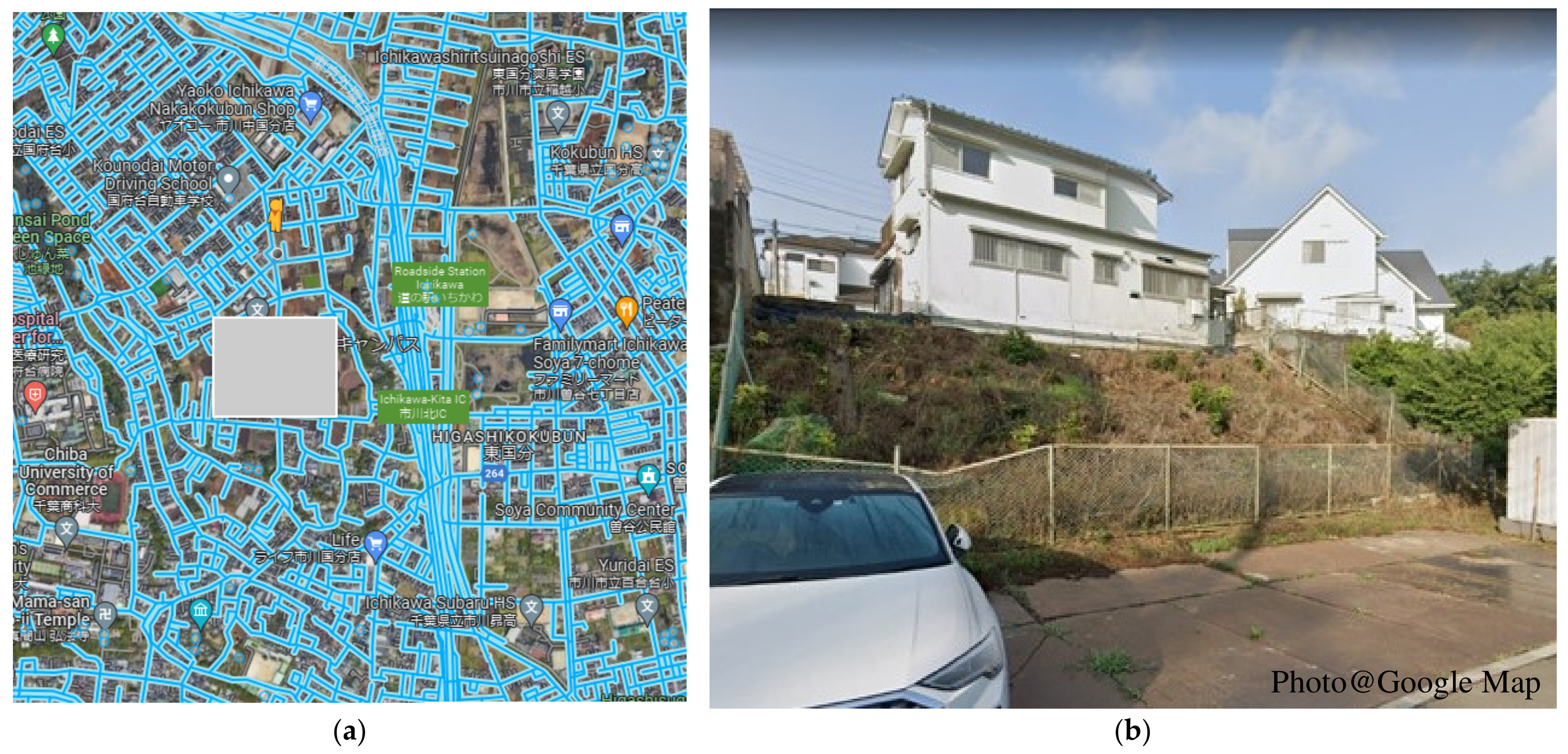
Figure 14.
Advantages of GSV in detecting and identifying IGSs: (a) a single person can perform this method, even with a drag-and-drop “pegman”; (b) IGSs can be easily observed in standard view. (The photos are taken from same location in Japan, so the names come with both English and Japanese).
Figure 14.
Advantages of GSV in detecting and identifying IGSs: (a) a single person can perform this method, even with a drag-and-drop “pegman”; (b) IGSs can be easily observed in standard view. (The photos are taken from same location in Japan, so the names come with both English and Japanese).
Table 1.
The quality level and number of photos collected in this study.
Table 1.
The quality level and number of photos collected in this study.
| Source | Location | Resolution (Pixels) | Total Photos Downloaded | Total Photos Have IGSs Detected |
|---|
| Google Street View | Ichikawa City, Japan | 2048 × 1024 * | ~80% | 15,429 | 3029 |
1344 × 672;
1408 × 449;
1664 × 832; | ~20% |
| Google Street View | Tan Binh and Phu Nhuan districts in HCMC, Vietnam | 1280 × 640;
1375 × 687;
1920 × 960;
2048 × 1024 | ~30% | 9124 | 204 |
| Lower resolutions ** | ~70% |
| Publisher’s Note: MDPI stays neutral with regard to jurisdictional claims in published maps and institutional affiliations. |
© 2022 by the authors. Licensee MDPI, Basel, Switzerland. This article is an open access article distributed under the terms and conditions of the Creative Commons Attribution (CC BY) license (https://creativecommons.org/licenses/by/4.0/).


