Optimal Regional Allocation of Future Population and Employment under Urban Boundary and Density Constraints: A Spatial Interaction Modeling Approach

Abstract

This paper develops an optimization modeling framework to select strategies of land development and population and employment densities for a growing metropolitan area. The modeling core involves a non-linear commuting model, which accounts for spatial structure variables and is empirically estimated by Tobit regression. This commuting model is then embedded into a non-linear optimization model that allocates increments in the population and employment (activities) to available land, while minimizing the total future commuting costs under various combinations of land expansion boundaries and population and employment densities. The resulting minimum cost surface is approximated via polynomial regression and combined with land development and congestion cost functions to derive the overall optimal strategy. These models are estimated and calibrated with data from the Census Transportation Planning Package (CTPP) and Auditor’s property database, and are applied to the Fredericksburg metropolitan area, Virginia. The results demonstrate that the optimal development densities are very sensitive to the congestion cost function. A land development strategy that allows for limited sprawl might be a smart policy to reduce both regional vehicle mile travel (VMT) and related congestion and pollution.

1. Introduction

1.1. Historical Overview of Urban Modeling

Accurately predicting the spatial pattern of population and economic activity is necessary for developing successful regional plans and policies. Computer-based urban simulation models originated in the U.S. in the 1950s’ metropolitan transportation studies and used geographic accessibility concepts. However, the attempts to build large-scale urban models failed over the next 15 years. After Lowry [1] introduced a comprehensive spatial interaction model called “The Lowry Model” to simulate location patterns of residential and commercial/service activities for a given pattern of basic (export manufacturing) employment locations, while accounting for accessibility, a renaissance in urban modeling took place, based on spatial interaction modeling (SIM), with initial formulations using the gravity model. During the 1960~1970s, the focus of SIM was primarily on population and activities. The 1980~1990s witnessed efforts at integrating land-use and transportation modeling. More recently, comprehensive models have involved environmental modeling, and the advent of the digital era, advances in computer technology, sophisticated spatial analysis methods, and the availability of big data, combined with geographic information systems (GIS), have generated new urban models.

In order to provide an appropriate background for this research, we critically review the literature on SIM, the relationship between SIM and planning optimization models, and the costs of urban sprawl and congestion. We then summarize the shortcomings of past research and outline the goals of this research.

1.2. Spatial Interaction Modeling: Structure and Variables

Spatial interaction modeling (SIM) represents various models that explain and predict spatial flows, including residence–workplace commuting, shopping travel, inter-city travel, migration, tourism, commodity flows, financial transactions, and various telecommunication forms. SIM ranges from the standard gravity model (GM), reflecting Newtonian physics, to entropy models to discrete spatial choice models. The basic GM is formulated as follows:

T_ij = kR_iW_j/D_ij^α

(1)

In this equation, T_ij is the flow from origin i to destination j, R_i and W_j are the measures of the sizes of the origin i and destination j, respectively, D_ij is the distance between them, and α is a positive parameter that represents the distance friction. The R_i and W_j variables are proxies for the abilities of the origin to generate flows and of the destination to attract them. Generalized versions of Equation (1) include several variables that characterize both the origin and destination, and several friction factors. This model has been termed as unconstrained SIM. The estimation of (1), subject to the given total outflows for all the origins and given total inflows for all the destinations, is termed as constrained or entropy SIM. The focus here is on the unconstrained case. These models consider aggregate flow data (e.g., the number of commuters between the origins and destinations). Another interpretation of SIM is related to discrete choice models (e.g., multi-nomial logit models), using disaggregate data at the level of the individual decision maker. Anas [2] argues that the gravity and discrete choice models are two equivalent views of the same problem. For reviews of the theory and applications of SIM, one can refer to the work of Sen and Smith [3], who discuss the theoretical foundations and practical applications of gravity models to commuting, and Nijkamp and Ratajczak [4], who review the relevance of gravitational principles in regional science and spatial economics, and address their application to trade flow analysis.

The above SIM approach suffers from the problem of independence from irrelevant alternatives. SIM models have been improved by incorporating variables that represent the effects of the spatial structure, thus eliminating the estimation bias of the friction parameters. Fotheringham [5] introduced a competing destination (CD) factor that measures the accessibility of any destination j to all (or a subset of) the other destinations. If the effect of CD is negative, competition to attract flows can be detected among the destinations; the closer destination j is to the other destinations, the smaller the flow terminating at j. If the effect of CD is positive, agglomeration effects can be observed among the neighboring destinations (e.g., a set of different brand stores within a shopping mall). Another approach to accounting for the spatial structure involves the intervening opportunities (IO) factor [6], which measures the accessibility of an origin to destinations located between the origin and the destination. IO measures the absorbing effects on the originating flow. Gitlesen and Thorsen [7] present an application of the CD concept to commuting modeling in Norway, while accounting for discontinuities in the road network.

Sirmans [8] is among the first to highlight the importance of incorporating various socio-economic determinants into SIM models, including cost, gender, race, income, age, and education and outlines the following points: (1) cost variables are expected to have a negative influence on commuting flows; (2) age variables are expected to have a negative influence on commuting flows, due to increased costs; (3) the higher the education level, the higher the commuting flows; (4) income variables are expected to have a positive influence on commuting flows; (5) race variables (percentages of minorities) are expected to have a negative influence on commuting flows. The results also point out that the determinants of commuting vary across gender.

Sandow [9] shows that women commute shorter distances than men. Sermons and Koppelman [10] also show that the presence of children, the occupation of the male worker in a household, and the last change in the female worker’s workplace are important determinants of gender differences in commuting behavior. Prashker et al. [11] investigated various factors that influence an individual’s choice of residence location, using a logit model, and showed the importance of area characteristics and commuting distance in selecting a residential location, with significant differences between genders. They also showed that commuting distance becomes less important with increasing income, education, and car ownership. O’Kelly et al. [12], using Irish data, show that commuting trip length varies by occupation and gender. Lin et al. [13] reviewed the impacts of socio-economic factors on commuting.

Another SIM research stream is the relationship between housing prices/locations, employment centers’ locations, and commuting. Kim et al. [14] developed an empirical model to show how housing prices, wages, and commuting times affect joint residential and workplace location choice. They show that residents trade lower housing costs for lower wages, and higher housing costs for higher wages. Wu [15] analyzed the impacts of employment and housing development on commuting in the Silicon Valley region and indicated that housing affordability and land-use patterns are important determinants of residential location choices and commuting flows, and that accessibility, local government expenditures, land availability, and ethnic background are important determinants of the spatial distribution of employment. Glenn et al. [16] show that commuting flows result not only from wage differentials and distances, but also from a spatial mismatch between the types of jobs and the categories of workers. Ahrens and Lyons [17], using a gravity model with Irish data, show that rising housing rents lead to longer commutes. Sohn [18] examined how commuting patterns reveal urban structures (where jobs and housings are located), by including locational variables (distance from the city center) for the origins and destinations of commuting flows in a modified gravity model.

1.3. Planning Optimization Models and Spatial Interaction Modeling

There have been various research efforts to design normative models for delineating more efficient urban patterns, including convex programming models that embed spatial interaction models within activity-allocation frameworks [19]. Kim [20] further expands this approach by adding alternative transportation systems. Some important works in this line of research include [21,22,23,24,25]. Prastacos’ POLIS model maximizes total locational surplus and combines the allocation of employment and a multi-modal transportation system. It is a programming formulation of the Lowry model and incorporates the location of basic employment with data from the San Francisco region.

Barber [26] uses the Lowry model reformulated in matrix form by Garin [27] to develop a linear goal programming model, which determines the basic employment distribution that minimizes deviations from target zonal populations. Using the newly distributed population, the model then estimates zone-specific service and retail employment. Barber [28] develops a linear programming model to allocate the future growth in basic employment to minimize total travel time. Basic employment, and hence basic land-use requirements, is the control variable, whereas service employment and population and their land-use requirements are not. The objective function reflects total travel time for all work- and home-based service trips.

More recent land-use allocation and transportation simulation models include those proposed by Ma et al. [29] and Samani et al. [30]. These models include gravity-based components of the ITLUP (integrated transportation and land-use planning) model, initially developed by Putnam [31]. Some recent studies focus on the relationship between accessibility and the spatial structure of economic activities. Wu et al. [32] evaluate the relationship between the spatial structure of medical resources and the accessibility of medical facilities in different traffic analysis zones and shed light on the potential optimal solutions for the spatial allocation and efficient utilization of medical services. Zhang et al. [33] scrutinize the relationship between the spatial pattern of roadway networks and the quality of business environments. Finally, one should mention the recent stream of multi-objective land-use optimization models, exemplified by [34,35]. However, these models do not incorporate the transportation system or transportation interactions (e.g., commuting), and built-up areas are not differentiated in terms of internal land use. The focus of these models is on sustainability and ecological protection.

1.4. Sprawl versus Compact City: Cost Assessment

The effect of urban sprawl on commuting patterns seems to be controversial. Some argue that sprawl has negative consequences for commuting, with longer commutes and congestion [36]. Ewing et al. [37] find no relationship between sprawl and commuting time. Weber and Sultana [38], using 1990 and 2000 Census Transportation Planning Package (CTPP) data for Birmingham, Alabama, differentiate workplace sprawl from residential sprawl, and examine the impact of employment sprawl on the commuting of White and Black workers. Their results show that workplace sprawl reduces commuting distances for those who commute to the sprawling areas and suggest that workers may be able to reduce their commutes as more workplaces relocate to suburban areas. However, workplace sprawl may increase commutes for those who may not be able to adjust their residential location. Variables found to influence commuting length include race, income, mode of transportation, location, population and household density, employment density, homeownership, and time leaving home for work [39].

Dunphy and Fisher [40] report that increasing density decreases the number of daily trips per person, but also assert that high density causes more congestion and pollution. Levinson and Kumar [41] test the influence of residential density on commuting patterns, and conclude that density is an important explanatory variable, with noticeable negative effects on the speed and distance of trips. They use 1980/1990 U.S. Census data and 1990/1991 Nationwide Personal Transportation Survey (NPTS) data. Auto travel time is negatively related to density below a density threshold (10,000 persons per square mile) and positively so above this threshold. O’Toole [42] indicates that there is no consensus about how much compact development reduces total driving and he suggests that the benefits of compact development are often likely to be overstated and its costs understated. The costs of compact development include loss of property rights, reduced geographic mobility, higher housing costs and lower home-ownership rates, higher taxes or reduced urban services to subsidize compact development, increased traffic congestion, and reduced economic mobility. Cambridge Systematics, Inc. [43] reports that congestion would be clearly a major result of a compact development plan and estimates that doubling densities from an average of 3000 people per square mile to an average of 7000 people would reduce per capita driving by less than 15 percent, but would still lead to a 100 percent increase in total vehicle travel miles. Without new road/highway expansion to accommodate this increased demand, there would be a large increase in regional congestion. Stevens [44] conducted a meta-regression analysis of the results of 46 studies to derive a clearer understanding of the influence of compact development on driving, and found a generally small, although significant, reduction in driving.

Air pollution has also been analyzed in the context of the sprawl/compactness debate. Emrath and Liu [45] show that the vehicle miles travelled (VMT) declines as the compactness of subdivisions increases, but with less efficient speeds. However, on balance, CO₂ emissions still tend to be lower in more compact developments. Stone [46], using data on 45 large U.S. metropolitan areas, shows that sprawling areas are associated with more ozone exceedances than more spatially compact metropolitan regions. Schindler and Caruso [47] develop a theoretical monocentric urban model to analyze the trade-off between traffic-based pollutant emissions and pollution exposure. Solving the model with parameters drawn from the literature, they find that emissions increase with sprawl and exposure increases with compactness, underscoring the difficulty in assessing compactness net benefits. Finally, Zhang et al. [48] show that there is a significant correlation between urban development patterns and PM_2.5 concentrations.

1.5. Summary and Research Goals

Although spatial interaction modeling of commuting has been the subjects of much urban research, there have not been many planning/optimization applications to residential and employment allocations that incorporate SIM. Both Barber’s and Prastacos’ models are essentially programming formulations of the Lowry model, where only basic employment is a control variable, with residential allocations automatically derived. In addition, few commuting models have incorporated SIMs and spatial structure factors. It is clear that improved SIMs should incorporate spatial structure effects in order to avoid the misspecification of conventional gravity models and that planning/optimization models should also consider land development costs and congestion/pollution costs, in addition to commuting costs.

Given the above shortcomings, the goals of this research are as follows:

• Develop a new SIM for commuting trip distribution, based on Tobit regression estimation [49] and including spatial structure variables measured by competing destinations (CD) [5] and intervening opportunity (IO) [6] factors. It is expected that incorporating these factors will better represent commuting behavior and commuting costs.
• Using the Tobit commuting SIM, develop a new commuting cost minimization model that simultaneously allocates target increments in the population and employment to geographical units across a city or metropolitan area under various scenarios of (a) population and employment densities (land consumption per resident and per employee) and (b) land availability in each geographical unit, as determined by the growth boundaries and environmental constraints. The results of this optimization include a minimum commuting cost surface, which is then to be estimated by polynomial regression, with the densities as independent variables.
• Combining the polynomial commuting cost model with estimated land development cost models and synthetic congestion cost models, develop a total cost minimization model to determine the optimal densities under various growth boundary scenarios and various parametric assumptions for the congestion cost functions.
• Use data on a specific U.S. metropolitan area to test the feasibility of the above-methodological goals. This would be a proof-of-concept goal, but is not intended to provide an actual plan for the local authorities of this metropolitan area.

2. Data and Methods

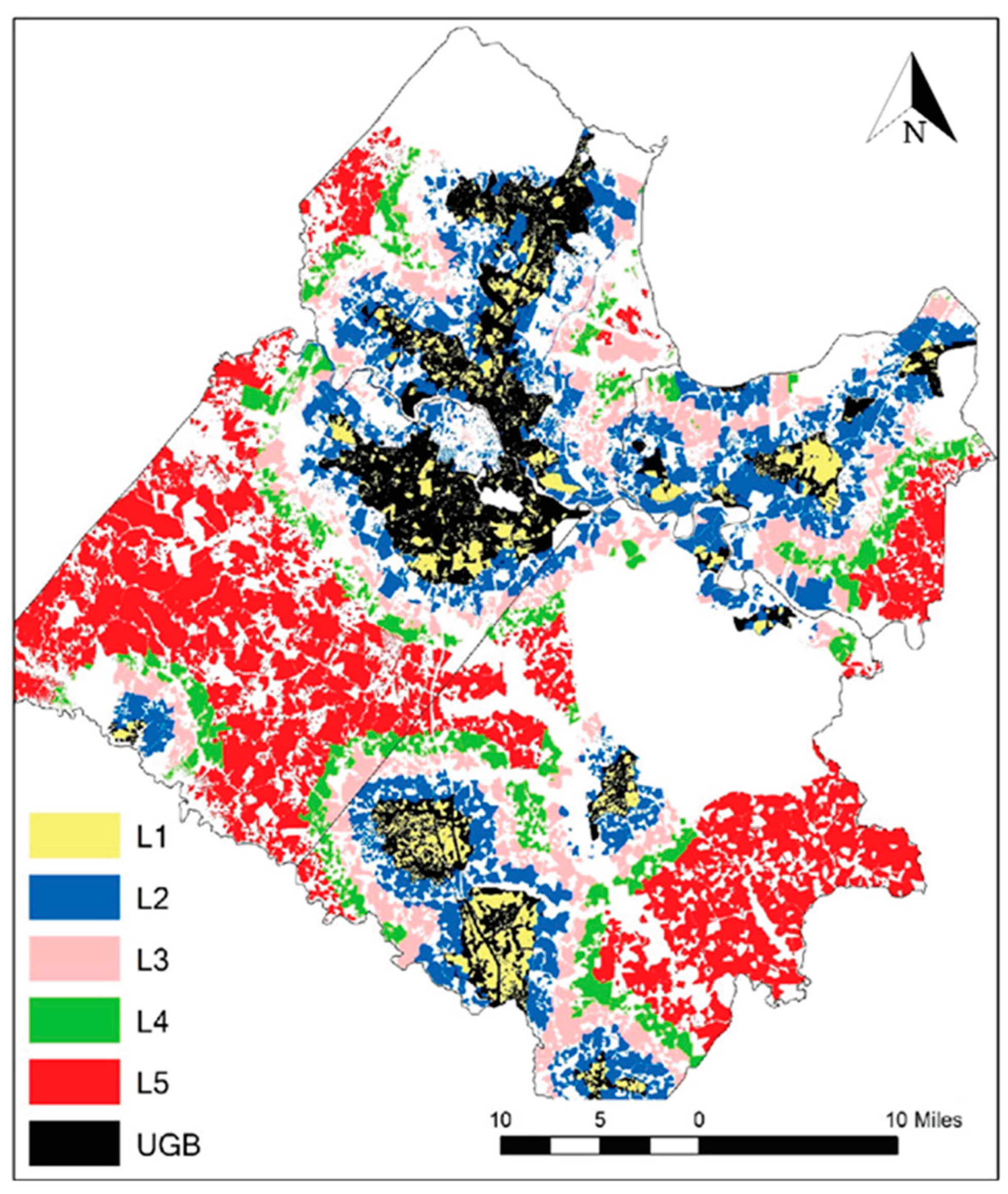
2.1. Overview of the Study Area

The Fredericksburg Area Metropolitan Planning Organization (FAMPO) was established in 1992, in accordance with Federal regulations, stating that “a metropolitan planning organization (MPO) shall be designated for each urbanized area with a population of more than 50,000 individuals.” To be classified as an urbanized area, a central place and any contiguous areas must have a density of at least 1000 persons per square mile. Based on the 1990 Census, an urbanized area consisting of the city of Fredericksburg and portions of Spotsylvania and Stafford counties met this threshold. FAMPO chose to expand its boundaries to include the three jurisdictions in their entirety. The Planning District 16 (George Washington Regional Commission—GWRC) in Virginia deals with FAMPO jurisdictions of two additional rural counties, King George and Caroline. For convenience, the terms “FAMPO region” and “George Washington Region” are used interchangeably in this paper. The location of FAMPO within Virginia is indicated in Figure 1.

The FAMPO region, because of its proximity to the rapidly growing suburbs of the Washington, D.C., metropolitan area (to the north) and the Richmond-Petersburg metropolitan area (to the south), is the fastest growing region in Virginia, with a 2006 population of 310,000 persons, nearly a third more than in 2000. The projections suggest that an additional 250,000 people will be living in FAMPO by 2035. As a result, the region is experiencing the growing pains related to sprawl, traffic safety and congestion. FAMPO’s central location and proximity to expanding employment opportunities has encouraged the significant migration of new residents, both to fill local jobs and to seek affordable housing and rural and lower density suburban lifestyles.

2.2. Data Sources

2.2.1. CTPP 2000

Most of the data are drawn from the 2000 Census Transportation Planning Package (CTPP), a set of special tabulations prepared for transportation planners, based on data from the decennial census. CTPP data are downloadable from the following website: CTPP Data—Transportation.org. It is the only Census product that summarizes data by place of work and provides information on travel flows between homes and workplaces. It provides summary tabulations for traffic analysis zones (TAZs) and other small geographic areas. The CTPP is divided into the following three parts: Part 1 includes residence-based data, summarizing worker and household characteristics; Part 2 includes place-of-work data; and Part 3 data includes data on commuting flows from residences to workplaces. The geographical unit of analysis in this research is the TAZ, and there are 188 TAZs in FAMPO. The year 2000 was the last year when the CTPP was produced by the Bureau of the Census, in collaboration with the Bureau of Transportation Statistics, using data from the Long Form survey (16% sampling). This decennial survey was cancelled by the U.S. Congress and replaced by the Annual Community Survey (ACS), with a sampling rate of 3%. Data derived from the ACS are more uncertain, hence the choice of the CTPP 2000 data. It is, however, important to emphasize that the goal of this paper is to present a new planning methodology and to use data to demonstrate its feasibility, and not to produce a plan to be used by FAMPO.

The 2000 population and employment distributions are mapped in Figure 2 and Figure 3. The highest population concentrations are located in the north of Stafford County (A); south of Route 3 and west of the I-95 interstate highway (B); and around the city of Fredericksburg, the center of the region (C). There are three employment clusters, which are as follows: the CBD of Fredericksburg (D); the Quantico military base located in the north of Stafford County (E); and Dahlgren, the site of a U.S. naval base located at the eastern corner of King George County (F).

Population and employment distribution across the FAMPO region are summarized by jurisdiction in

Table 1. FAMPO Region Population and Employment in 2000.

Jurisdiction	Population	%	Employment	%
Caroline	22,120	9.2%	1945	2.3%
Fredericksburg	19,275	8.0%	19,760	23.2%
King George	16,805	7.0%	9912	11.6%
Spotsylvania	90,405	37.5%	26,521	31.1%
Stafford	92,460	38.4%	27,059	31.8%
Total	241,065	100.0%	85,197	100.0%

. Two urban counties, Spotsylvania (37.5%) and Stafford (38.4%), function as major residential areas and also, together with the city of Fredericksburg, provide most of the regional employment (31.1% Spotsylvania; 31.8% Stafford; and 23.2% Fredericksburg).

Zone-to-zone and jurisdiction-to-jurisdiction flows for 2000 are summarized in

Table 2. Commuting Flows (Number of Commuters) in 2000.

			Flow	%
FAMPO	Internal		7125	10.61
	TAZ-to-TAZ		60,023	89.39
Jurisdiction	Caroline	Internal	1261	1.88
		Jurisdiction-to-Jurisdiction	203	0.30
	Fredericksburg	Internal	4056	6.04
		Jurisdiction-to-Jurisdiction	12,699	18.91
	King George	Internal	4314	6.42
		Jurisdiction-to-Jurisdiction	3173	4.73
	Spotsylvania	Internal	15,863	23.62
		Jurisdiction-to-Jurisdiction	6377	9.50
	Stafford	Internal	11,469	17.08
		Jurisdiction-to-Jurisdiction	7733	11.52
Total Flow			67,148	100%

. Fredericksburg displays high interactions with the other jurisdictions (18.91%), while Spotsylvania has the highest level of internal flows (23.62%). A high share of the people living in Stafford work there (17.08%).

2.2.2. Property Data

Real estate data have been collected from the planning departments of local governments and combined into a regional data set to maintain consistency and comparability. The collected assessment data all apply to 2006. The following variables are available for each record that characterizes a parcel: parcel I.D.; land use; total land value; total building value; total property value; size (acre); jurisdiction; TAZ I.D. Average values per parcel for size, land value, building value, and property value by jurisdiction are provided in Table 3. These data can be obtained from the following Tax Assessor Offices:

• Real Estate Taxes|Fredericksburg, VA—Official Website (fredericksburgva.gov);
• Stafford County, VA (staffordcountyva.gov);
• Assessment Office, Spotsylvania County, VA; Real Estate, Caroline County, VA;
• Real Estate, King George County, VA (kinggeorgecountyva.gov).

Table 3. Average Parcel Data in 2006.

	Residential Property				Workplace Property
Jurisdiction	Average Size (Acre)	Average Property Value (USD)	Average Land Value (USD)	Average Building Value (USD)	Average Size (Acre)	Average Property Value (USD)	Average Land Value (USD)	Average Building Value (USD)
Caroline	2.3658	220,462	47,598	162,618	5.3395	576,642	144,972	304,321
Fredericksburg	0.3525	260,831	53,914	178,740	1.2749	945,372	388,820	506,586
King George	3.2624	245,225	72,054	167,082	4.5400	517,810	196,227	271,619
Spotsylvania	1.3127	147,640	65,580	82,059	14.0769	3,717,248	3,330,981	386,267
Stafford	1.1375	372,153	102,621	269,531	3.3182	1,241,485	479,788	761,687
FAMPO	1.4254	247,782	77,390	167,696	8.3923	2,309,510	1,809,006	481,376

Table 3. Average Parcel Data in 2006.

	Residential Property				Workplace Property
Jurisdiction	Average Size (Acre)	Average Property Value (USD)	Average Land Value (USD)	Average Building Value (USD)	Average Size (Acre)	Average Property Value (USD)	Average Land Value (USD)	Average Building Value (USD)
Caroline	2.3658	220,462	47,598	162,618	5.3395	576,642	144,972	304,321
Fredericksburg	0.3525	260,831	53,914	178,740	1.2749	945,372	388,820	506,586
King George	3.2624	245,225	72,054	167,082	4.5400	517,810	196,227	271,619
Spotsylvania	1.3127	147,640	65,580	82,059	14.0769	3,717,248	3,330,981	386,267
Stafford	1.1375	372,153	102,621	269,531	3.3182	1,241,485	479,788	761,687
FAMPO	1.4254	247,782	77,390	167,696	8.3923	2,309,510	1,809,006	481,376

2.3. Variables

2.3.1. Dependent Variable

The TAZ-to-TAZ flow table from CTPP 2000 Part 3 includes a large number of zero values. The number of potential commuting connections (all records) is 35,344 (188 × 188), including 188 intra zonal flows. Among these connections, 90.2% (31,875) have zero flow values.

Table 4. Descriptive Statistics for Non-Zero Flows in 2000.

Variable	N	Mean	Standard Deviation	Minimum	Maximum
F: flow	3469	19.35	34.17	4.00	990.00
P: population	3469	2332.27	2659.69	15.00	15,730.00
E: employees	3469	1683.79	1687.31	4.00	6415.00
D: distance	3469	10.51	6.97	0.42	41.07

and

Table 5. Descriptive Statistics for Zero Flows in 2000.

Variable	N	Mean	Standard Deviation	Minimum	Maximum
F: flow	31875	0	0	0	0
P: population	31875	1167.99	1765.41	0	15,730.00
E: employees	31875	319.25	734.31	0	6415.00
D: distance	31875	18.76	9.25	0.70	50.53

present the descriptive statistics for these flows. Records with zero flows embody useful information, and therefore cannot be discarded in statistical analyses.

2.3.2. Independent Variables

The potential independent variables have been directly drawn from CTPP Parts 1 and 2 or are derived from these primary variables. These variables can be grouped as follows: Group A: residence-based variables (CTPP 2000 Part 1); Group B: workplace-based variables (CTPP 2000 Part 2); Group C: impedance variable; Group D: spatial structure variables.

Group A

The larger the population of a residential TAZ (P), the larger the commuting flow expected to originate from it. Gender differences have been shown to affect human behavior; therefore, the share of the male population (P_M_RES) is selected. Unemployment rates are also likely to have negative impacts on flows; therefore, the total (P_UNEMP_RES) and male (P_MUNEMP_RES) unemployment rates are selected. A high percentage of people driving alone to work implies more cars on the roads, and therefore larger commuting flows. High car-pooling rates can be expected to reduce flows; therefore, the following variables are selected:

-

Percentage of workers driving alone from their residence (P_DA_RES);

-

Percentage of workers carpooling from their residence (P_CP_RES);

-

Percentage of male workers driving alone from their residence (P_MDA_RES);

-

Percentage of male workers carpooling from their residence (P_MCP_RES).

Age variables, such as the percentages of residents aged 25 to 64 (P_AGE25_64) and of residents aged 65 + (P_AGE65PLUS), are likely to have positive and negative impacts on commuting flows, respectively. Employment occupation may have an effect on flows, although the direction of the effect is a priori unclear. The following variables are selected:

-

Percentage of residents in sales or service occupations (P_OCC1_RES);

-

Percentage of residents in clerical or administrative support occupations (P_OCC2_RES);

-

Percentage of residents in manufacturing, construction, or maintenance occupations (P_OCC3_RES);

-

Percentage of residents in professional, managerial, or technical occupations (P_OCC4_RES);

-

Percentage of male residents in sales or service occupations (P_MOCC1_RES);

-

Percentage of male residents in clerical or administrative support occupations (P_MOCC2_RES);

-

Percentage of male residents in manufacturing, construction, or maintenance occupations (P_MOCC3_RES);

-

Percentage of male residents in professional, managerial, or technical occupations (P_MOCC4_RES).

It has been argued that low-income minorities experience poor employment opportunities due to underprivileged accessibility. In order to test such effects, and particularly race impacts on travel patterns, the following variables are selected:

-

Percentage of Hispanic or Latino residents (P_HIS_RES);

-

Percentage of White residents (P_WHT_RES);

-

Percentage of Black or African American residents (P_BLK_RES).

A higher share of White residents within a population, probably associated in part with higher income, is likely to produce larger commuting flows. The share of disabled people (P_DIS_RES) is likely to have a negative relationship with flows. Income and earnings are likely to have a positive effect on flows. To test these hypotheses, the following variables are selected:

-

Percentage of resident households with an income of USD 75,000 or more in 1999 (P_HINC_RES);

-

Median resident household income (MHI_RES);

-

Percentage of resident workers with high earnings (USD 50,000+) in 1999 (P_HERN_RES);

-

Percentage of resident workers below the poverty level in 1999 (P_POV_RES);

Home ownership is measured by the following variables:

-

Percentage of households with self-owned housing (P_OWNSELF_RES);

-

Percentage of households with owned housing with and without a mortgage (P_OWN_RES).

High vehicle availability is measured by the percentage of households with 3 or more vehicles (P_3VEH_RES). High housing occupancy rates are measured by the percentage of occupied housing units (P_OCCU_RES). Higher education rates are measured by the percentage of residents with a bachelor’s degree or higher (HEDU_RES). These variables are also likely to have positive effects on commuting flows. Descriptive statistics for Group A variables across the 188 TAZs of FAMPO are presented in

Table 6. Descriptive Statistics for Group A Variables.

Variable	N	Mean	Median	Standard Deviation	Minimum	Maximum
P	188	1282.26	625.00	1903.91	0.0	15,730.0
P_DA_RES	188	0.7601	0.7782	0.1498	0.0	1.000
P_BLK_RES	188	0.1525	0.1165	0.1421	0.0	0.674
P_OCC1_RES	188	0.1618	0.1627	0.0844	0.0	0.600
P_OCC2_RES	188	0.1858	0.1920	0.0914	0.0	0.455
P_OCC3_RES	188	0.2150	0.2000	0.1140	0.0	0.580
P_OCC4_RES	188	0.1769	0.1700	0.1002	0.0	0.495
P_M_RES	188	0.4981	0.4912	0.0918	0.0	0.984
P_UNEMP_RES	188	0.0214	0.0165	0.0256	0.0	0.150
P_MUNEMP_RES	188	0.0189	0.0000	0.0305	0.0	0.200
P_CP_RES	188	0.1480	0.1334	0.1031	0.0	0.700
P_MDA_RES	188	0.7538	0.7802	0.1866	0.0	1.000
P_MCP_RES	188	0.1517	0.1303	0.1305	0.0	1.000
P_MOCC1_RES	188	0.1232	0.1172	0.1031	0.0	0.667
P_MOCC2_RES	188	0.0837	0.0817	0.0696	0.0	0.400
P_MOCC3_RES	188	0.3279	0.3094	0.1731	0.0	1.000
P_MOCC4_RES	188	0.2047	0.2000	0.1375	0.0	0.695
P_HIS_RES	188	0.0185	0.0000	0.0309	0.0	0.192
P_WHT_RES	188	0.7876	0.8220	0.1699	0.0	1.000
P_DIS_RES	188	0.1429	0.1250	0.1028	0.0	0.600
P_HINC_RES	188	0.4013	0.4006	0.2163	0.0	1.000
MHI_RES	188	54,720.88	52,675.00	18,921	0	109,770
P_HERN_RES	188	0.2071	0.2032	0.1140	0.0	0.5052
P_POV_RES	188	0.0218	0.0112	0.0331	0.0	0.250
P_OWNSELF_RES	188	0.1881	0.1667	0.1385	0.0	1.000
P_OWN_RES	188	0.7895	0.8546	0.2137	0.0	1.125
P_3VEH_RES	188	0.3406	0.3354	0.1614	0.0	0.769
P_OCCU_RES	188	0.9131	0.9486	0.1428	0.0	1.000
HEDU_RES	188	0.0384	0.0341	0.0381	0.0	0.388

.

Group B

The level of employment (EMP) at the workplace (destination) is likely to have a positive impact on attracted flows. It is also likely that higher rates of full-time workers lead to higher flows. This is measured by the percentage of people who worked 40+ hours per week in 1999 at their workplace (P_Full_EMP). Vehicle availability is also likely to increase commuting flows, and it is measured by the percentage of people with 2 or more vehicles at their workplace (P_Veh2plus_EMP). Variables that are likely to have a negative relationship with flows include the following:

-

Percentage of employees below the poverty level (P_BlwPov_EMP);

-

Mean travel time (MTT_EMP);

-

Percentage of workers with low earnings (P_LERN_EMP);

-

Percentage of workers that carpool (P_CarPool_EMP).

The percentages of workers with high earnings (P_HEARN_EMP), driving alone (P_DA_EMP), and arriving at the morning peak period (P_AM7_10_EMP) are likely to have positive effects on commuting flows. Type-of-industry variables are likely to have mixed impacts and include the following:

-

Percentage of workers in manufacturing (P_Mfg_EMP);

-

Percentage of workers in wholesale trade (P_WhlTrd_EMP);

-

Percentage of workers in retail trade (P_RetTrd_EMP);

-

Percentage of workers in service industries (P_serv_EMP);

-

Percentage of workers in public administration (P_Pub_EMP).

Descriptive statistics for these variables are presented in

Table 7. Descriptive Statistics for Group B Variables.

Variable	N	Mean	Median	Standard Deviation	Minimum	Maximum
EMP	188	453.1755	75.0000	964.605	0.0000	6415.0
P_Full_EMP	188	0.3321	0.3099	0.2435	0.0000	1.0000
P_Veh2Plus_EMP	188	0.7334	0.8265	0.2895	0.0000	1.0000
P_BlwPov_EMP	188	0.0364	0.0108	0.0698	0.0000	0.6667
MTT_EMP	188	24.712	25.000	15.369	0.0000	102.3
P_LERN_EMP	188	0.3681	0.3631	0.2498	0.0000	1.0000
P_CarPool_EMP	188	0.0883	0.0809	0.0923	0.0000	0.4000
P_Mfg_EMP	188	0.0379	0.0000	0.0948	0.0000	0.7500
P_WhlTrd_EMP	188	0.0192	0.0000	0.0480	0.0000	0.4000
P_RetTrd_EMP	188	0.0864	0.0106	0.1413	0.0000	1.0000
P_serv_EMP	188	0.3687	0.3637	0.3014	0.0000	1.0000
P_Pub_EMP	188	0.0327	0.0000	0.0777	0.0000	0.4427
P_Finan_EMP	188	0.0561	0.0000	0.1341	0.0000	1.0000

.

Group C

Distances have been computed as Euclidian distances (miles) between the zone centroids.

Table 8. Descriptive Statistics for Inter-TAZ Distances.

Variable	N	Mean	Median	Standard Deviation	Minimum	Maximum
D	35,344	17.947	17.380	9.379	0.420	50.530

provides descriptive statistics for the inter-TAZ distances (D).

Group D

The intervening opportunity (IO) and the competing destinations (CD) factors are based on employment. The CD factor measures the accessibility of destination j to other destinations in the neighborhood of j, while the IO factor measures the accessibility of origin i to other origins in the neighborhood of i. The following three different types of IO factors have been proposed by Guldmann [50]: the IO circle, IO sector, and IO corridor. In this research, the IO circle, as originally used by [6], is retained. The neighborhoods for the IO and CD factors of a given TAZ are circles of a 10-mile radius centered on the centroid of the TAZ. A higher IO factor is expected to reduce outgoing commuting flows (negative relationship), while the CD factor could have either negative or positive effects on commuting flows. A positive effect suggests the presence of agglomeration forces at the destination, and a negative one suggests the presence of competition forces. The IO and CD factors are defined mathematically as follows:

$$\mathrm{IO}={\displaystyle \sum _k{E}_k{d}_{ik}^{\gamma }}, \to k\ne i \mathrm{a}\mathrm{n}\mathrm{d} k \in \mathrm{N}\mathrm{e}\mathrm{i}\mathrm{g}\mathrm{h}\mathrm{b}\mathrm{o}\mathrm{r}\mathrm{h}\mathrm{o}\mathrm{o}\mathrm{d} \mathrm{o}\mathrm{f} \mathrm{T}\mathrm{A}\mathrm{Z} i$$

(2)

$$\mathrm{CD}={\displaystyle \sum _l{E}_l{d}_{jl}^{\epsilon }}, \to l\ne j \mathrm{a}\mathrm{n}\mathrm{d} l \in \mathrm{N}\mathrm{e}\mathrm{i}\mathrm{g}\mathrm{h}\mathrm{b}\mathrm{o}\mathrm{r}\mathrm{h}\mathrm{o}\mathrm{o}\mathrm{d} \mathrm{o}\mathrm{f} \mathrm{T}\mathrm{A}\mathrm{Z} j$$

(3)

In order to illustrate the computation of the IO and CD factors, one must consider Figure 4, with the origin TAZ 5 and destination TAZ 17. The neighborhood TAZs for TAZ 5, within a 10-mile radius, are {2,6,7,8}. Similarly, the neighborhood TAZs for TAZ 17 are {6,15,18}. The factors are computed as follows:

$${\mathrm{IO}}_{5,17}={\displaystyle \sum _{\begin{array}{l}k\ne 5\\ k\in \left\{2,6,7,8\right\}\end{array}}{E}_k{d}_{5,k}^{\gamma }}$$

(4)

$${\mathrm{CD}}_{5,17}={\displaystyle \sum _{\begin{array}{l}l\ne 17\\ l\in \left\{6,15,18\right\}\end{array}}{E}_l{d}_{17,l}^{\epsilon }}$$

(5)

2.4. Statistical and Optimization Methodology

Spatial interaction models (SIMs) of commuting flows are estimated with, as explanatory variables, the population P_i at the origin i, the employment E_j at the destination j, several socio-economic variables characterizing either i or j (X…, Y…), the distance d_ij, and competing destinations (CD_j) and intervening opportunity (IO_i) variables that characterize the spatial structure. If F_ij is the commuting flow between i and j, a general SIM can be calculated as follows:

$$F_{ij}=f(P_i,E_j,d_{ij},X,\dots ,Y,\dots ,\mathrm{C}{\mathrm{D}}_j,\mathrm{I}{\mathrm{O}}_i)$$

(6)

Tobin [49] analyzed household expenditures on durable goods, while taking into account the fact that expenditures cannot be negative. He proposed a regression method applied to data with censored values, which became known as the Tobit model. The basic dependent variable in this research, commuting flow, cannot be negative, and any examination of an actual flow matrix shows that many flows are equal to zero. The Tobit model is a reasonable approach to deal with this problem.

The conceptual basis for using the Tobit model is based on resident worker (RW) utility maximization. One must assume that the RW has a choice among multiple origin–destination (O–D) trips (by virtue of residential and employment location decisions), and that only one O–D trip turns out to be positive, with all the others turning out to be negative at the utility maximum. These negative values are not observed and become zero values in terms of actual trips. The observed flows can then be viewed as the sums of these individual commuting decisions, and the zero flow values represent the censored unobserved negative values. Therefore, the latent variable of the Tobit model captures both positive and negative sums of commuting flows. With standard regression approaches with only positive observed values, the information embodied in zero flow observations is lost. Ordinary least squares (OLS) estimation applied to a truncated sample will be biased and inconsistent. The Tobit model allows the explicit inclusion of zero commuting observations. This is particularly important if there are large volumes of zero observations.

The latent variable In the Tobit is specified as follows:

$${\widehat{F}}_{ij}=\beta x_{ij}+\epsilon$$

(7)

The actual flow $F_{ij}$ is defined as

$$\begin{array}{l}{F}_{ij}=\{\begin{array}{ll}{\widehat{F}}_{ij}=\beta x_{ij}+\epsilon & \mathrm{if} {\widehat{F}}_{ij}>0\\ 0& \mathrm{if}{\widehat{F}}_{ij}\le 0\end{array}\\ \epsilon ~N(0,{\sigma }^2)\end{array}$$

(8)

${\widehat{F}}_{ij}$ is the latent variable that represents the “desired” commuting flows, which can be negative. A Tobit linear commuting flow SIM can be formulated as follows:

$$F_{ij}=a_0+{\displaystyle \sum _i{a}_i{X}_i}+{\displaystyle \sum _j{b}_j{X}_j}+{\displaystyle \sum _{i,j}{c}_{ij}{Z}_{ij}}$$

(9)

where a_i, b_j, and c_ij are the parameters, X_i and X_j are the variables that characterize the origin i and destination j, Z_ij represents the impedance variables (e.g., distance, time and price) and F_ij is the commuting flow.

$P_i^0$ and $E_j^0$ represent the existing (base year) population and employment in zones i and j, respectively. The population and employment allocation problem involves the optimal allocation of total population and employment increments, $\Delta P_T$ and $\Delta E_T$, to all zones where land is available for a certain target year. x_i and z_j are the population and employment increments allocated to zones i and j, and Z and X are the corresponding vectors. In addition, ULP is the population density (land area per new resident), ULE is the employment density (land area per new employee), and LAND_i is the land available in zone i for new residents and new employees. The parameters ULP and ULE uniformly apply to all the geographical units. However, the model could be easily modified to test for spatially varying density scenarios. If C_ij is the fixed unit commuting cost between i and j, a general total commuting cost minimization model can be as follows:

$$\mathrm{Minimize} Z={\displaystyle \sum _{i,j}{C}_{ij}{F}_{ij}}$$

(10)

This is subject to

$${\displaystyle \sum x_i=\Delta P_T}$$

(11)

$${\displaystyle \sum z_j=\Delta E_T}$$

(12)

$$F_{ij}\ge {\widehat{F}}_{ij}(P_i^0+x_i,E_j^0+z_j,d_{ij},X\dots Y\dots ,\mathrm{C}{\mathrm{D}}_j\left(\mathit{Z}\right),\mathrm{I}{\mathrm{O}}_i\left(\mathit{X}\right))$$

(13)

ULP.xi + ULE.zi ≤ LAND_i

(14)

$$F_{ij}\ge 0 x_i\ge 0 z_j\ge 0$$

(15)

The objective (10) is to find the minimum total commuting cost. Constraint (11) guarantees that the sum of all increments in the population equals the total population increment, and constraint (12) ensures the same for employment. The Tobit constraint (13) defines the commuting flow between i and j, and constraint (15) guarantees that F_ij = 0 when the right-hand side of constraint (13) is negative. ULP and ULE are the given parameters in the optimization model, but can be varied in the context of scenario analyses. Constraint (14) simply states that the land to be used for new residents and employees in zone I cannot exceed the land available. In the specific case of the FAMPO region with 188 zones (TAZs), this model has 36,097 variables and 35,911 constraints.

However, minimizing the total commuting costs cannot be the sole objective of the model. Other costs need to be considered. For instance, compact development is assumed to reduce pollution emissions by reducing driving and housing a higher percentage of people in multi-family and mixed-use developments at more central locations, reducing utility costs and utilizing more transit and fewer highways. Land development costs would be smaller in such developments. However, some argue that compact developments can be more costly than often estimated [42], because compact cities may increase emissions by increasing roadway congestion. These costs are often neglected. In addition, compact development may entail higher housing costs and lower homeownership rates, reduced geographic and economic mobility, higher taxes, reduced urban services, higher consumer costs, etc. A more general cost function can then be stated as follows:

TOTAL COST = commuting cost (TCOM)

+ land development cost (LDC)

+ congestion cost (TCON)

(16)

All the costs in (16) were formulated in terms of both residential and employment densities, or, alternatively, in terms of unit land consumption per resident (ULP) and per employee (ULE). The higher the ULP and ULE, the lower the corresponding densities. Commuting costs and land development costs increase, and congestion costs decrease with ULP and ULE. These cost curves, and the total cost curve are illustrated in Figure 5. The LDC would include all annualized land/building costs for both employment and the population. The TCOM represents the annual commuting cost. The TCON represents the congestion costs for both the population and employment. Within the given ranges of ULP and ULE, the total cost function (TCD) will point to the optimal ULP and ULE that minimize the total cost.

3. Results

3.1. Tobit Regression

The estimation of the final Tobit model with SAS^TM procedure QLIM (qualitative and limited dependent variable models) is the outcome of a multi-step exploratory process. The first estimated model (Model 1) involved only three independent variables that appear in most gravity models, which are as follows: population (P), employment (EMP) and distance (D). All the coefficients turned out to be highly significant (p < 0.0001), with the expected positive sign for P and EMP, and the expected negative sign for D, and with R² = 0.297 and Pseudo-R² = 0.042. The Pseudo-R² is defined as follows:

$$R_{MF}^2=\frac{LRT}{LRT*}=\frac{(l_M-l_0)}{(l_{MAX}-l_0)}=1-\frac{l_M}{l_0},$$

(17)

where LRT is the likelihood ratio statistic; $l_M$ is the log-likelihood value of the model; $l_0$ is the log-likelihood value if the non-intercept coefficients are restricted to zero; $l_{MAX}$ is the maximum possible likelihood. One can refer to [51] for a discussion on the Pseudo-R² for limited dependent variable models.

The second step was to add the spatial structure variables IO and CD to Model 1. Since the IO and CD factors involve additional parameters (exponents of distance) that need to be estimated, a grid sensitivity analysis was conducted to search for the optimal parameter set. For both γ (IO factor) and ε (CD factor), the range (−2.0, 0) was selected, as typical in the literature, with a 0.1 increment. Hence, 400 combinations of γ and ε values were evaluated in this sensitivity analysis. The combination of γ = −0.1 and ε = −0.3 yielded the highest log-likelihood, as well as the highest Pseudo-R². All the five variables of this model (Model 2) turned out to be very significant (p < 0.0001), with a negative sign for IO (as expected) and a positive sign for CD, pointing to agglomeration effects at the destination.

The third step was to add socio-economic variables, as listed in Groups A and B, to Model 2. The following variables improved in Model 2 (significance and sign; overall performance) and were retained in Model 3: P_DA_RES, P_BLK_RES, P_OCC1_RES, P_OCC2_RES, P_OCC3_RES, P_OCC4_RES, P_Mfg_EMP, P_WhlTrd_EMP, P_RetTrd_EMP, P_Finan_EMP, P_serv_EMP, and P_Pub_EMP. However, none of the INCOME, GENDER and AGE-related variables turned out to be significant. For Model 3, R² = 0.355, and Pseudo-R² = 0.121.

The final model (Model 4) expands on Model 3 by introducing quadratic terms. The following significant quadratic terms were selected:

E2 = EMP * EMP

(18)

P2 = P * P

(19)

POPEMP = P * EMP

(20)

EMPCD = EMP * CD

(21)

Table 9. Tobit Parameter Estimation of Model 4.

Parameter	Estimate	Standard Error	t-Value	Approx Pr > |t|
Intercept	−80.267754	4.532873	−17.71	<0.0001
P	0.011133	0.000426	26.13	<0.0001
EMP	0.027680	0.001218	22.73	<0.0001
D	−3.966485	0.158067	−25.09	<0.0001
IO_E	−0.000324	0.000024329	−13.33	<0.0001
CD_E	0.000160	0.000035343	4.53	<0.0001
P_DA_RES	28.859800	3.679491	7.84	<0.0001
P_BLK_RES	9.602796	3.023634	3.18	0.0015
P_OCC1_RES	23.840650	6.515631	3.66	0.0003
P_OCC2_RES	12.881209	5.595655	2.30	0.0213
P_OCC3_RES	16.725051	4.991596	3.35	0.0008
P_OCC4_RES	17.346662	5.671378	3.06	0.0022
P_Mfg_EMP	36.628397	4.083194	8.97	<0.0001
P_WhlTrd_EMP	53.338335	7.888539	6.76	<0.0001
P_RetTrd_EMP	22.840645	3.075172	7.43	<0.0001
P_Pub_EMP	43.681025	5.569463	7.84	<0.0001
P_Serv_EMP	19.602157	1.794940	10.92	<0.0001
P_Finan_EMP	21.147896	2.754040	7.68	<0.0001
P2	−0.000000662	3.1856992 × 10−8	−20.78	<0.0001
E2	−0.000002661	0.000000158	−16.87	<0.0001
D2	0.048005	0.004843	9.91	<0.0001
POPEMP	0.000002331	0.000000113	20.68	<0.0001
EMPCD	−0.000000109	1.807805 × 10−8	−6.03	<0.0001
R-square	0.4657
Pseudo-R2	0.2394
Log-likelihood	−20,466

represents the parameter estimates of Model 4, with R² = 0.466, and Pseudo-R² = 0.239. Model 4 has stronger performance criteria than Model 3, pointing to the non-linear relationship between commuting flows and the variables P, EMP, D, and CD. The more workers that drive alone to their workplace (P_DA_RES), the higher the flow. The magnitude of this variable coefficient is relatively high (33.11). The share of Black citizens within a population (P_BLK_RES) also has a positive impact on flows. The Black population in the region is a highly educated and affluent middle-class community, hence its mobility and likely positive impact on flows. The occupation and industry variables display the expected signs. The more residents with sales or service (P_OCC1_RES) or clerical or administration (P_OCC2_RES) occupations, the larger the commuting flows. These occupations have stronger impacts than the other two occupations. The percentages of workers in manufacturing, wholesale trade, retail trade, fire, service, and public administration occupations all have positive impacts on commuting flows. Wholesale trade (P_WhlTrd_EMP) and public administration (P_Pub_EMP) have the largest coefficients, 90.08 and 89.72, respectively, followed by manufacturing (55.57), retail trade (45.22), finance industries (36.17), and service occupations (22.13). This result is consistent with the existence of large regional distribution centers, such as CVS and UPS, as well as government and military workers.

3.2. Minimizing Commuting Costs in the Allocation of Population and Employment

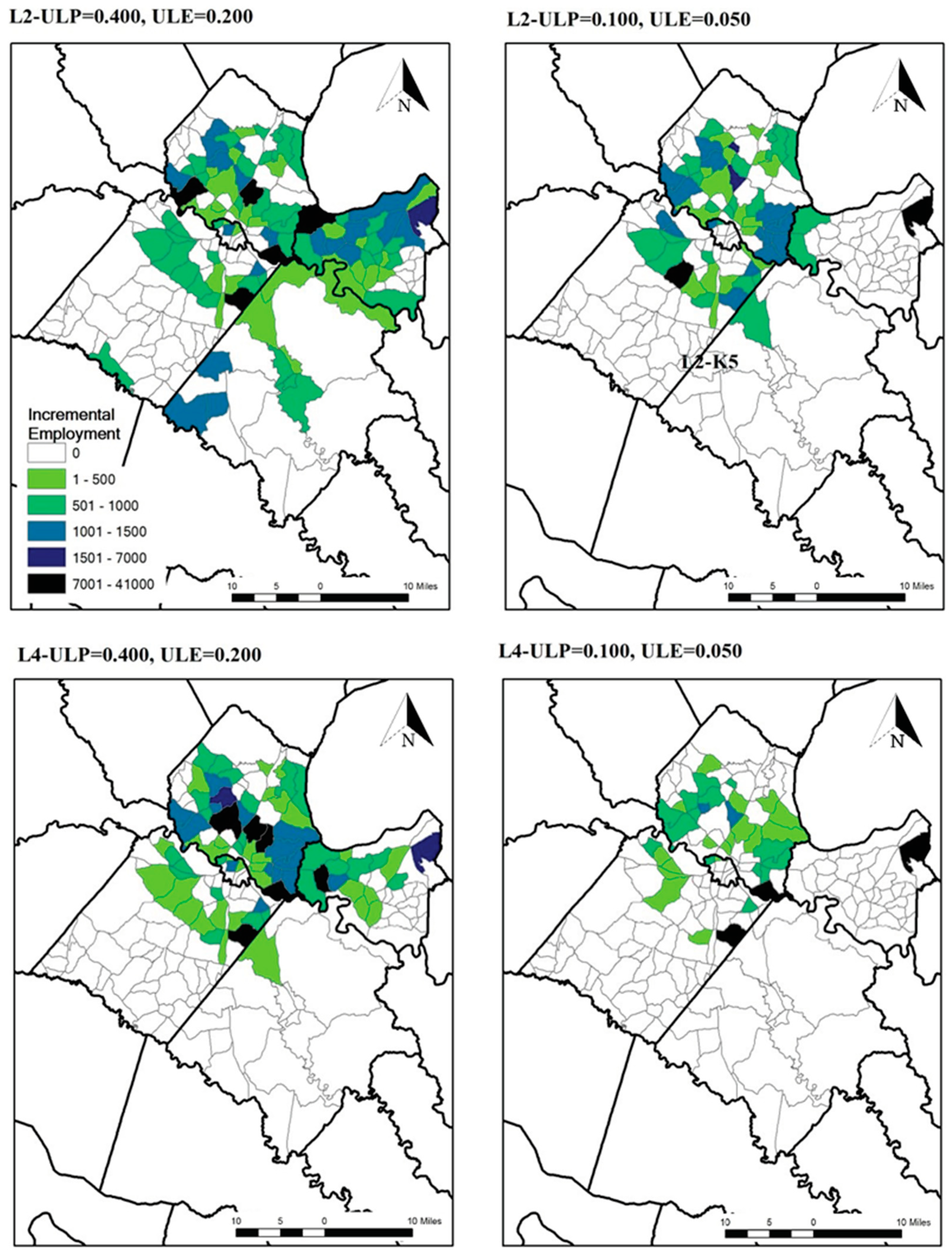
3.2.1. Scenarios

The control totals for population and employment for the horizon year 2035 were obtained from the Virginia Employment Commission (VEC) and the GWRC. The model allocates the total regional increments in the population and employment to the 188 TAZs of FAMPO, while assuming that the existing population and employment levels remain at their current locations. The existing and target population and employment levels are presented in

Table 10. Target Population and Employment.

Jurisdiction		2035
		Employment	Population
Caroline County		14,216	47,007
Fredericksburg		43,679	29,852
King George County		17,821	40,744
Spotsylvania County		62,551	236,885
Stafford County		69,574	238,208
Total GWRC (PD 16)		207,841	592,696
2000 (Existing)		Increments
Employment	Population	ΔE	ΔP
85,197	241,065	122,644	351,631

.

Vacant land is made available for any future housing and employment development, except in physically, environmentally, and historically sensitive lands. Developed/developable land is delineated using a geographical information system (GIS) and is classified into the following five categories: existing residential developed land, existing commercial developed land, existing industrial developed land, undevelopable land, and vacant developable land. Vacant developable land is selected for possible further development expansion.

Each jurisdiction in FAMPO has primary settlement/growth area boundaries in its comprehensive long-range plan. These boundaries are not exactly the same as the urban growth boundaries (UGB) that control urban expansion into farm and forest lands in Portland, Oregon. One can also refer to [52] for information on rigid vs. flexible boundaries in the context of urban growth/development boundaries and an application for delineation. They are not used to control growth, but rather to define long-term city boundaries. However, this land-use control tool functions rather well in managing urban growth in the region. It has been observed that new housing developments built since 2000 have taken place around and within these boundaries. The following five land development scenarios were initially considered: L1—within UGB (35,535 acres); L2—within UGB + 1.0 mile (171,241 acres); L3—within UGB + 2.0 mile (252,508 acres); L4—within UGB + 3.0 mile (305,921 acres); L5: all developable land (503,412 acres). These scenarios are illustrated in Figure 6. After initial exploratory modeling, the scenarios L1 and L5 were discarded as too restrictive and too unconstrained, respectively. The Scenarios L2 and L4 were then retained as sufficiently contrasted scenarios to provide insights into the impact of land availability.

While rural areas have higher average land consumption per resident (ULP) and employee (ULE), in the range of (2~3) acres, urban areas are characterized by denser developments in the range of (0.1~0.2) acres. All the areas of the FAMPO parcels of land currently occupied by the population and employment have been summed up at the TAZ level. Using the existing (2000) TAZ population and employment data, the following region-wide average densities have been derived: ULP = 0.429 acres and ULE = 0.223 acres. Using the increments $\Delta P$ and $\Delta E$ for population and employment, and the above density values, the total amount of land required by 2035 would be 178,199 acres. It is assumed that, in the future (target year 2035), the average ULP and ULE values will be smaller than the current values, and the following 9 × 9 grid of values is considered:

• ULP: (0.10–0.50) by 0.05 increments
• ULE: (0.05–0.25) by 0.025 increments

Except for the variables POP and EMP, which are endogenous to the optimization model, all the other variables of the Tobit model are also assumed to remain constant over time. It is also assumed that the share variables (P_DA_RES, P_BLK_RES, P_OCC1_RES, P_OCC2_RES, P_OCC3_RES, P_OCC4_RES, P_Mfg_EMP, P_WhlTrd_EMP, P_RetTrd_EMP, P_Pub_EMP, P_Serv_EMP, and P_Finan_EMP) remain constant and equal to their current values.

3.2.2. Model Formulation

The optimization model presented in Section 2.4 (Equations (10)–(15)) is adjusted as follows. First, the commuting travel costs are proxied by the total vehicle miles traveled (VMT). If D_ij is the distance between TAZs i and j, the objective function to be minimized is as follows:

$$Z={\displaystyle \sum _i{\displaystyle \sum _j{D}_{ij}{F}_{ij}}}$$

(22)

Second, Equation (13) is reformulated as Equation (23) by using the Tobit parameters presented in Table 9, in which $P_i^0$ is the existing 2000 population in TAZ i, $E_j^0$ is the existing 2000 employment level in TAZ j, ${(P_i^0+x_i)}^2$ is the square of the final population (existing plus increment) in TAZ i; ${(E_j^0+z_j)}^2$ is the square of the final employment level (existing plus increment) in TAZ j.

The model is a non-linear program because of the squares and products of the decision variables. The optimization is implemented with the general algebraic modeling system (GAMS) and with the non-linear solver CONOPT.

However, because of its non-linearity and non-convexity, this model only provides local optima, and a global optimum search is infeasible, due to the model size (36,097 variables and 35,911 constraints). In other words, the optimal solution obtained for any set of values for ULP and ULE may vary depending on the initial starting point of the optimization algorithm. Thus, the only way to deal with this problem is to repeatedly solve the model with the CONOPT solver, and to select the solution with the smallest objective function (OF) value. The results presented below are the outcomes of this process.

$$\begin{array}{l}{F}_{ij}\ge -80.267754+ 0.011133\cdot (P_i^0+x_i)+ 0.027680\cdot (E_j^0+z_j)- 3.966485D_{ij}^{}\\ -0.000324\cdot \left({\displaystyle \sum _{\begin{array}{l}k\ne i\\ k\in Neighborhood\_of\_i\end{array}}\left(E_k^0+z_k\right)D_{ik}^{-0.3}}\right)+0.000160\cdot \left({\displaystyle \sum _{\begin{array}{l}l\ne j\\ l\in Neighborhood\_of\_j\end{array}}\left(E_l^0+z_l\right)D_{jl}^{-0.1}}\right)\\ +28.859800\cdot {(P\_DA\_RES)}_i+ 9.602796\cdot {(P\_BLK\_RES)}_i\\ + 23.840650\cdot {(P\_OCC1\_RES)}_i+ 12.881209\cdot {(P\_OCC2\_RES)}_i\\ +16.725051\cdot {(P\_OCC3\_RES)}_i+ 17.346662\cdot {(P\_OCC4\_RES)}_i\\ + 36.628397\cdot {(P\_MFG\_EMP)}_j+ 53.338335\cdot {(P\_WhlTrd\_EMP)}_j\\ + 22.840645\cdot {(P\_\mathrm{Re}tTrd\_EMP)}_j+ 43.681025\cdot {(P\_Pub\_EMP)}_j\\ + 19.602157\cdot {(P\_Serv\_EMP)}_j+ 21.147896\cdot {(P\_Finan\_EMP)}_j\\ -0.000000662\cdot {(P_i^0+x_i)}^2-0.000002661\cdot {(E_j^0+z_j)}^2+ 0.048005D_{ij}^2\\ + 0.000002331\cdot (P_i^0+x_i)\cdot (E_j^0+z_j)-0.000000109\cdot (E_j^0+z_j)\cdot \left({\displaystyle \sum _{\begin{array}{l}l\ne j\\ l\in Neighborhood\_of\_j\end{array}}\left(E_l^0+z_l\right)D_{jl}^{-0.1}}\right)\end{array}$$

(23)

3.2.3. Optimization Results

In order to contrast the VMT minimization results between high- and low-density scenarios, two sets of ULP and ULE pairs, including (1) high density: ULP = 0.10; ULE = 0.050 and (2) low density: ULP = 0.40; ULE = 0.200, were selected among the 9 × 9 grid of values and combined with the L2 and L4 land development scenarios.

The optimal TAZ-to-TAZ flows have been summarized into jurisdiction-to-jurisdiction flows, as presented in

Table 11. Optimal Commuting Flows by Jurisdiction.

Scenario L2		To
ULP = 0.400	ULE = 0.200	CR	FR	KG	SF	SP
From	CR	1000	3830	4849	7395	4223
	FR	0	961	33	528	802
	KG	9	2205	5531	2891	2369
	SF	0	4481	1575	10,991	3796
	SP	40	5855	1545	6215	10,695
Scenario L2		To
ULP = 0.100	ULE = 0.050	CR	FR	KG	SF	SP
From	CR	29	1582	382	967	1463
	FR	0	812	0	341	562
	KG	0	350	92	20	282
	SF	0	2016	0	3251	1322
	SP	0	2848	0	1417	3936
Scenario L4		To
ULP = 0.400	ULE = 0.200	CR	FR	KG	SF	SP
From	CR	136	288	1349	2304	1415
	FR	0	780	48	472	592
	KG	0	813	1057	1405	919
	SF	0	3836	1146	9045	2751
	SP	0	4886	1544	5245	8266
Scenario L4		To
ULP = 0.100	ULE = 0.050	CR	FR	KG	SF	SP
From	CR	2	7	0	0	23
	FR	0	763	0	357	549
	KG	0	0	17	0	0
	SF	0	1787	0	4030	1170
	SP	16	4038	0	2075	3837

CR: Caroline; FR: Fredericksburg; KG: King George; SF: Stafford; SP: Spotsylvania.

. The optimal values of the OF, total flows and average commuting distance are summarized in

Table 12. Optimal Objective Function, Total Flow, and Average Commuting Distance.

Land Scenario		Density Scenario
		ULP = 0.400	ULP = 0.100
		ULE = 0.200	ULE = 0.050
L2	Objective function	838,777	113,647
	Total flows	81,819	21,671
	Average commuting distance	10.25	5.24
L4	Objective function	473,283	106,347
	Total flows	48,294	18,671
	Average commuting distance	9.80	5.70

. The OF and the total flow decrease with more land available and a higher density, which indicates that a land-use policy that confines new developments within UGBs would significantly increase regional VMT. This large flow increase leads to increased congestion and air pollution costs, which are addressed in Section 3.3.4.

Figure 7 displays the optimal TAZ-to-TAZ flows, while Figure 8 and Figure 9 present the optimal allocations of the incremental population and employment, respectively. As more land becomes available, the incremental population and employment tend to move away towards rural areas. In addition, as density increases, more people and jobs are located closer to the urban cores. An interesting observation is that, for a given density scenario, when less land is available (e.g., L2 rather than L4), this requires higher levels of commuting flows. The L2 UGB requirement leads to more spatial separation of population and employment than under less restrictive land-use controls (L4). Thus, a tight UGB strategy does not appear to be the best way to reduce VMT, and the resulting congestion and air pollution. Another interesting observation is that moving from low to high density and from L2 to L4 leads to the southern TAZs being more and more disconnected in terms of flows, with most of the inter-TAZ and inter-jurisdictional flows concentrated in the northern TAZs. Compact development scenarios evidently result in the highest volumes of commuting flows. This could be a justification for further transit development and use. Most of the observed commuting flows involve private car transportation, and other modes of transportation are not explicitly considered, because their shares are currently very small.

3.3. Minimizing All Costs in the Allocation of Population and Employment

3.3.1. Overview of Costs

The previous VMT-minimizing results demonstrate that density constraints are critical in determining the distribution of populations and employment, and therefore must be carefully considered. For any given land development strategy, the highest possible densities allow for minimizing commuting costs. However, commuting costs do not represent all urban and regional costs, which also include land development costs and congestion/pollution costs. The purpose of this section is to develop and optimize such an expanded cost function (TDC), taken as the sum of the commuting costs (TCOM), the total land development costs (LDC), and the total congestion costs (TCON).

3.3.2. Estimation of the Commuting Cost Surface

In Section 3.2.3, the total commuting cost (TCOM) was minimized under two density scenarios. However, it is now necessary to consider the variations in TCOM over a wider range of density values. A 9 × 9 grid analysis (ULP = 0.10~0.50 by 0.05 increments; ULE = 0.050~0.250 by 0.025 increments) of density scenarios is used to build up the relationship between the commuting cost and ULP and ULE. The general approach is to solve the VMT minimization model over these 81 density parameters (ULP, ULE) for land development strategies L2 and L4, and then to approximate the resulting cost surfaces through polynomial regression analysis. The normalized minimum VMT values for each pair of ULP and ULE are presented in

Table 13. Minimum Commuting Costs for a 9 × 9 grid of ULP and ULE values.

Normalized
Land Scenario L2		ULE
		0.050	0.075	0.100	0.125	0.150	0.175	0.200	0.225	0.250
ULP	0.10	12.21	15.05	17.09	17.17	17.23	19.56	20.26	21.67	22.12
	0.15	15.06	16.24	17.56	18.32	20.61	22.26	22.99	23.18	23.44
	0.20	26.31	27.15	28.03	28.16	28.42	28.92	29.06	29.15	29.55
	0.25	33.14	39.99	40.34	41.25	41.32	42.06	44.21	45.06	45.30
	0.30	40.62	46.95	53.61	57.55	59.47	61.18	62.55	64.59	66.17
	0.35	48.17	60.51	66.65	71.39	79.09	81.80	85.00	87.99	91.40
	0.40	53.13	64.22	70.87	78.52	80.79	85.27	90.12	100.00
	0.45	63.43	76.50	80.40
	0.50
Normalized
Land Scenario L4		ULE
		0.050	0.075	0.100	0.125	0.150	0.175	0.200	0.225	0.250
ULP	0.10	18.96	20.82	21.69	25.55	26.88	27.71	28.01	28.72	29.08
	0.15	23.10	23.41	26.63	29.99	32.82	36.03	36.15	36.26	36.39
	0.20	31.63	35.46	38.57	39.61	39.90	40.13	40.33	40.50	40.73
	0.25	39.40	40.17	41.09	41.72	42.26	42.71	43.14	43.56	43.97
	0.30	44.12	46.64	51.31	53.13	53.93	54.71	55.55	56.36	57.20
	0.35	48.18	51.69	56.12	65.54	69.32	71.19	71.22	72.31	73.40
	0.40	49.13	56.64	64.89	71.43	80.24	83.10	84.40	85.64	87.05
	0.45	51.15	59.24	65.18	74.43	81.43	83.41	85.23	86.67	88.28
	0.50	55.52	63.55	72.26	80.09	88.76	92.80	95.45	97.63	100.00

Note: Red cells correspond to unfeasible solutions.

. Normalized values provide a clearer picture of the variations in the minimum VMT. For Scenario L2, the maximum value (100) represents VMT = 930,741; for Scenario L4, the corresponding value is VMT = 560,790. VMT values under L2 are larger than those under L4. This is reasonable because L4 is less constraining (provides more location opportunities), which should lead to a lower VMT for any given set of (ULP, ULE) values.

The normalized commuting cost surfaces are illustrated in Figure 10. The surface for L2 displays sudden drops at certain values of ULP and ULE, due to infeasibility. The VMT values increase as the ULP and ULE increase. As expected, the VMT is minimized when the ULP and ULE are the smallest. The surfaces suggest that the VMT is more sensitive to the ULP than to ULE. The relationship between VMT and ULP and ULE for each land development strategy is estimated using a third-order cubic polynomial regression analysis and the results are presented in

Table 14. Results of 3rd Order Regression of TCOM over ULP and ULE.

Variables	Land Development Strategy
	L2	L4
Intercept	188,109 (1.71) *	100,497 (2.16) *
ULP	−3,410,307 (−3.34) **	−377,350 (−1.07)
ULE	2,816,147 (1.89) *	117,457 (0.17)
ULP × ULP	19,994,468 (5.65) **	3,921,962 (3.54) **
ULE × ULE	−14,772,237 (−1.68) *	2,136,213 (0.48)
ULP × ULE	−4,477,808 (−0.93)	878,521 (0.52)
ULP × ULP × ULP	−26,345,984 (−6.61) **	−5,919,163 (−5.02) **
ULE × ULE × ULE	31,053,141 (1.72) *	−3,265,161 (−0.35)
ULP × ULP × ULE	24,799,246 (3.94) **	9,630,043 (4.90) **
ULP × ULE × ULE	−6,222,188 (−0.62)	−13,204,059 (−3.36) *
R2	0.987	0.983

( ) t-statistics; * significant at 90% level, two-tailed test; ** significant at 99% level, two-tailed test.

.

As the models minimize the total commuter mile flows (Equation (22)), it is necessary to convert this quantity into the corresponding annual commuting cost, with the following equation:

$$TCOM=CPM\times ND\times {\displaystyle \sum _i{\displaystyle \sum _j{d}_{ij}{F}_{ij}}}$$

(24)

where CPM is the average commuting cost per person mile, and ND is the number of commuting days per year. CPM is estimated at USD 0.202 by dividing the 2005 purchases of cars and trucks and the spending on gas and oil (USD 988.2 billions), by the 2005 number of person travel miles (4884.557 billions of vehicle miles). In order to annualize the total commuting cost, the average number of workdays per year (ND) is calculated by assuming 2 weeks of vacation (10 days) and 10 days of federal holidays. Hence, ND = 240 days (50 weeks × 5 days–10 days).

3.3.3. Estimation of Land Development Costs

In order to develop land development cost functions for residence and workplace locations, with the ULP and ULE as determinants, parcel-level property values and developed acres data are drawn from the 2006 (4th quarter) Real Estate database that is used by local governments for tax assessment (Section 2.2.2). These data are aggregated at the TAZ level in order to match them with population and employment data. Land development cost functions, which involve acreage, population, and employees, are constructed as follows:

                                           Total property value (land + building) = f (residential acreage; population)

(25)

Total property value (land + building) = g (commercial + industrial + retail + office
acreage; employees)

(26)

The following three functional forms have been considered: (1) linear–linear; (2) log–log; and (3) log–linear. The log–log specification resulted in the highest R². However, because the ULP and ULE are the basic variables in the commuting flow function TCOM, the land development cost functions were re-estimated, in log–log form, with ULP and ULE as determinants, together with population P_2006 and employment E_2006. As the densities involve the ratios of acreages to population or employment, the same information is embodied in the new formulations. Furthermore, the exponents of P_2006 and E_2006 must be equal to 1 to avoid scale effects with regard to these variables. This homogeneity allows the estimated functions to be applied to any increment in the population and employment. The new regression results are presented in

Table 15. Regression Results for Land Development Cost Functions.

Land Development Cost (Residential)				Land Development Cost (Employment)
Intercept	11.218	262.90 (<0.0001)	R2 0.85	Intercept	10.810	93.39 (<0.0001)	R2 0.78
LN(P_2006)	1.000	Infty (<0.0001)		LN(E_2006)	1.000	Infty (<0.0001)
LN(ULP)	0.014	0.34 (0.7311)		LN(ULE)	0.502	10.40 (<0.0001)
RESTRICT	16.899	2.37 (0.0173)		RESTRICT	98.442	5.01 (<0.0001)

.

Therefore, the total cost of development for the increments $\Delta P$ and $\Delta E$ are as follows:

$$\mathrm{Population}: \mathrm{LDCP}=e^{11.218}\cdot \Delta P\cdot UL{P}^{0.014}$$

(27)

$$\mathrm{Employment}: \mathrm{LDCE}=e^{10.810}\cdot \Delta E\cdot UL{E}^{0.502}$$

(28)

In order to annualize these costs, the equivalent annual cost (EAC) formula obtained from the Board of Governors of the Federal Reserve System is used, with the following equation:

EAC = (Asset Price × IR)/(1 − (1 + IR)^(−N))

(29)

• IR = average mortgage interest rate over 1997~2006 = 6.71% = 0.0671
• N = number of periods = 30 years (normal mortgage payment period)

The annualized functions (27) and (28) are adjusted with the multiplier 0.078.

3.3.4. Congestion Cost Synthetic Functions

High-density, compact cities can entail traffic congestion costs, reduced urban services, air pollution and noise costs, etc. These costs can be assumed to decrease as density decreases. However, they are not easily statistically estimated due to the lack of necessary data. Here, these costs are assumed to be related to population, employment, and land consumptions, with the following synthetic functional forms:

TCONP = K1*∆P*(ULP** − b)

(30)

TCONE = K2*∆E*(ULE** − d)

(31)

where b, d, K1 and K2 are positive parameters.

Consistent with the theories, these costs decline with increasing ULP and ULE values (decreasing densities). The parameters K1 and K2 impact the height of the cost curves, whereas b and d impact their steepness.

3.3.5. Total Development Cost Minimization

Therefore, the annualized total development cost, TDC, is as follows:

TDC = TCOM + LDCP + LDCE + TCONP + TCONE

(32)

The allocated population and employment increments, ∆P and ∆E, are fixed. They are implicit in the commuting cost function, and explicit in the other functions, where they serve as given parameters. Hence, each of the cost components is only a function of the inverse densities ULP and ULE. Therefore,

TDC = TDC (ULP, ULE)

(33)

For instance, TDC with land strategy L2 is as follows:

$$\begin{array}{l}TDC=0.202\times 240\times (188109-3410307\times ULP+2816147\times ULE\\ +19994468\times UL{P}^2-14772237\times UL{E}^2-4477808\times ULP\times ULE\\ -26345984\times UL{P}^3+31053141\times UL{E}^3+24799246\times UL{P}^2\times ULE-6222188\times ULP\times UL{E}^2)\\ +\frac{(e^{11.218}\times \Delta P\times UL{P}^{0.014}\times 0.0671)}{(1-{(1+0.0671)}^{-30})}+\frac{(e^{10.810}\times \Delta E\times UL{E}^{0.502}\times 0.0671)}{(1-{(1+0.0671)}^{-30})}\\ +K1\times \Delta P\times UL{P}^{-b}+K2\times \Delta E\times UL{E}^{-d}\end{array}$$

(34)

A similar function for land strategy L4 is also easily formulated, but is not presented here. The optimal values ULP* and ULE* that minimize TDC depend upon the values of the congestion cost function parameters K1, K2, b, and d. The optimal ULP* and ULE* are obtained over the following grid of values for K1, K2, b, and d:

• K1 = 0.1, 0.3, 0.5;
• K2 = 0.1, 0.3, 0.5;
• b = 1.0, 3.0, 5.0;
• d = 1.0, 3.0, 5.0.

The optimal values of the development densities (ULP and ULE) are obtained by solving a simple two-variable optimization problem over a grid of 81 combinations of values for K1, K2, b, and d. In addition, the upper and lower bounds of the ULP and ULE are included in the model to be consistent with the bounds used in estimating the TCOM functions. The model is as follows:

Minimize TDC (ULP, ULE)

(35)

s.t.

0.100 ≤ ULP ≤ 0.500

(36)

0.050 ≤ ULE ≤ 0.250

(37)

For a given set of K1, K2, b, and d values, the optimal ULP and ULE values that minimize the total cost TDC are presented in

Table 16. Grid Analysis for Optimal ULP and ULE—L2 Case.

			K1
			0.1		0.3		0.5
K2	b	d	ULP	ULE	ULP	ULE	ULP	ULE
0.1	1.0	1.0	0.1000 L	0.0500 L	0.1000 L	0.0500 L	0.1000 L	0.0500 L
		3.0	0.1000 L	0.0805	0.1000 L	0.0805	0.1000 L	0.0805
		5.0	0.1000 L	0.2211	0.1000 L	0.2211	0.1000 L	0.2211
	3.0	1.0	0.1447	0.0500 L	0.1930	0.0500 L	0.2206	0.0500 L
		3.0	0.1443	0.0805	0.1917	0.0803	0.2186	0.0801
		5.0	0.1435	0.2213	0.1876	0.2212	0.2121	0.2209
	5.0	1.0	0.3135	0.0500 L	0.5000 U	0.0500 L	0.5000 U	0.0500 L
		3.0	0.3089	0.0793	0.5000 U	0.0763	0.5000 U	0.0763
		5.0	0.2952	0.2194	0.3594	0.2174	0.3989	0.2160
0.3	1.0	1.0	0.1000 L	0.0500 L	0.1000 L	0.0500 L	0.1000 L	0.0500 L
		3.0	0.1000 L	0.1108	0.1000 L	0.1108	0.1000 L	0.1108
		5.0	0.1000 L	0.2500 U	0.1000 L	0.2500 U	0.1000 L	0.2500 U
	3.0	1.0	0.1447	0.0500 L	0.1930	0.0500 L	0.2206	0.0500 L
		3.0	0.1439	0.1108	0.1905	0.1105	0.2168	0.1103
		5.0	0.1435	0.2500 U	0.1872	0.2500 U	0.2113	0.2500 U
	5.0	1.0	0.3135	0.0500 L	0.5000 U	0.0500 L	0.5000 U	0.0500 L
		3.0	0.3051	0.1090	0.5000 U	0.1042	0.5000 U	0.1042
		5.0	0.2932	0.2500 U	0.3551	0.2500 U	0.3917	0.2500 U
0.5	1.0	1.0	0.1000 L	0.0500 L	0.1000 L	0.0500 L	0.1000 L	0.0500 L
		3.0	0.1000 L	0.1285	0.1000 L	0.1285	0.1000 L	0.1285
		5.0	0.1000 L	0.2500 U	0.1000 L	0.2500 U	0.1000 L	0.2500 U
	3.0	1.0	0.1447	0.0500 L	0.1930	0.0500 L	0.2206	0.0500 L
		3.0	0.1438	0.1285	0.1899	0.1283	0.2158	0.1280
		5.0	0.1435	0.2500 U	0.1872	0.2500 U	0.2113	0.2500 U
	5.0	1.0	0.3135	0.0500 L	0.5000 U	0.0500 L	0.5000 U	0.0500 L
		3.0	0.3031	0.1265	0.5000 U	0.1205	0.5000 U	0.1205
		5.0	0.2932	0.2500 U	0.3551	0.2500 U	0.3917	0.2500 U

L: Lower bound; U: upper bound.

and

Table 17. Grid Analysis for Optimal ULP and ULE—L4 Case.

			K1
			0.1		0.3		0.5
K2	b	d	ULP	ULE	ULP	ULE	ULP	ULE
0.1	1.0	1.0	0.1000 L	0.0500 L	0.1000 L	0.0500 L	0.1000 L	0.0500 L
		3.0	0.1000 L	0.0810	0.1000 L	0.0810	0.1000 L	0.0810
		5.0	0.1000 L	0.2218	0.1000 L	0.2218	0.1000 L	0.2218
	3.0	1.0	0.1476	0.0500 L	0.2064	0.0500 L	0.2412	0.0500 L
		3.0	0.1470	0.0809	0.2048	0.0807	0.2387	0.0806
		5.0	0.1474	0.2223	0.2030	0.2227	0.2346	0.2228
	5.0	1.0	0.3399	0.0500 L	0.4456	0.0500 L	0.5000 U	0.0500 L
		3.0	0.3351	0.0801	0.4273	0.0794	0.5000 U	0.0787
		5.0	0.3248	0.2226	0.3991	0.2220	0.4423	0.2215
0.3	1.0	1.0	0.1000 L	0.0500 L	0.1000 L	0.0500 L	0.1000 L	0.0500 L
		3.0	0.1000 L	0.1108	0.1000 L	0.1108	0.1000 L	0.1108
		5.0	0.1000 L	0.2500 U	0.1000 L	0.2500 U	0.1000 L	0.2500 U
	3.0	1.0	0.1476	0.0500 L	0.2064	0.0500 L	0.2412	0.0500 L
		3.0	0.1466	0.1107	0.2037	0.1106	0.2368	0.1104
		5.0	0.1480	0.2500 U	0.2036	0.2500 U	0.2351	0.2500 U
	5.0	1.0	0.3399	0.0500 L	0.4456	0.0500 L	0.5000 U	0.0500 L
		3.0	0.3316	0.1097	0.4170	0.1089	0.4783	0.1081
		5.0	0.3243	0.2500 U	0.3973	0.2500 U	0.4391	0.2500 U
0.5	1.0	1.0	0.1000 L	0.0500 L	0.1000 L	0.0500 L	0.1000 L	0.0500 L
		3.0	0.1000 L	0.1281	0.1000 L	0.1281	0.1000 L	0.1281
		5.0	0.1000 L	0.2500 U	0.1000 L	0.2500 U	0.1000 L	0.2500 U
	3.0	1.0	0.1476	0.0500 L	0.2064	0.0500 L	0.2412	0.0500 L
		3.0	0.1465	0.1281	0.2032	0.1280	0.2360	0.1279
		5.0	0.1480	0.2500 U	0.2036	0.2500 U	0.2351	0.2500 U
	5.0	1.0	0.3399	0.0500 L	0.4456	0.0500 L	0.5000 U	0.0500 L
		3.0	0.3299	0.1272	0.4126	0.1262	0.4676	0.1254
		5.0	0.3243	0.2500 U	0.3973	0.2500 U	0.4391	0.2500 U

L: Lower bound; U: upper bound

with the land availability strategy L2 (UGB + 1-mile buffer) and L4 (UGB + 3-mile buffer), respectively. The results show that the optimal ULP and ULE vary, depending on the form of the congestion cost functions, which depend on the parameters K1, K2, b, and d. The ULP and ULE values marked with L and U represent the lower and upper bounds, respectively. The lower bound characterizes the highest density, and the upper bound demonstrates the lowest density.

For example, if K1 = 0.1, K2 = 0.1, b = 1.0, and d = 1.0 in the L2 case, then the optimal ULP and ULE values that minimize the total cost TDC are the lower bounds (ULP: 0.1000; ULE: 0.0500), which means that, for these congestion cost functions, the highest density strategy (compact development) for both residences and workplaces is optimal. However, if the congestion function is characterized by the parameters K1 = 0.1, K2 = 0.1, b = 5.0, and d = 5.0, then the optimal ULP and ULE values (ULP: 0.2952; ULE: 0.2194) demonstrate a lower density. Under this scenario, allowing sprawl to some extent may be the most appropriate strategy. It is also interesting to note that the optimal value of ULE hits its upper bound (ULE: 0.2500) in many cases, especially when d = 5.0 (steep function) and K2 ≥ 0.3 (higher intercept), representing a high congestion cost for workplace locations, which suggests that the suburbanization of workplaces can help to minimize TDC. When b = 1.0 (low steepness) for the congestion cost function for residential locations, ULP hits its lower bound (0.1000), irrespective of the values of the other parameters. Similarly, when d = 1.0 (low steepness) for the congestion cost function for workplace locations, ULE hits its lower bound (0.0500). These lower bounds point to the advisability of compact development for residences and workplaces. The results demonstrate that the form of the congestion function plays an important role in determining the optimal values of ULP and ULE.

4. Conclusions and Discussion

Using a Tobit commuting model that was empirically estimated with data for the FAMP region, Virginia, a normative planning model has been developed, incorporating alternative land development and density scenarios. Various growth management policy scenarios have been tested and compared. The results, expressed in terms of population and employment spatial patterns and expected commuting flows, demonstrate that tighter growth control policies increase system-wide commuting costs and flows, and do not necessarily reduce the average trip distances. The density constraints are critical in determining the distribution of populations and employment and must be carefully considered. The results also show that spatial structure variables are indeed important in estimating the Tobit model. The commuting cost minimization model has been expanded to include land development costs and congestion costs. The results demonstrate that the optimal development densities are very sensitive to the form of the congestion cost function and the land availability scenarios (growth boundaries). When the congestion function is not steep, a compact development strategy for residences and workplaces is advisable. However, with increasing steepness and level of the congestion functions, a land development strategy that allows for some sprawl minimizes the total urban development costs. The proposed optimization approach could be used for policy analysis. Since government policies, such as land-use controls and the provision of transportation infrastructure, play a major role in shaping cities, this approach could contribute to a better understanding of the dynamics of urban economies and allows planners to show the implications of policy scenarios to decision makers.

What are the contributions of this research to the literature on land-use pattern studies and policies? In the following section, we discuss three contribution areas, including spatial interaction modeling (SIM), land-use optimization, and the debate on sprawl versus compact development. First, the literature review in Section 1.2 shows that commuting SIMs that use data on commuting flows and land uses have a long history in both statistical estimation and policy simulation. However, we believe that the use of the Tobit model, which accounts for the information embodied in zero flows, the large number of potential residential and employment variables, and the spatial structure variables, all contribute to the innovative nature of this SIM. Second, the optimization framework that accounts for the commuting, land development, and congestion/pollution costs is, we believe, unique in the land-use optimization literature, as discussed in Section 1.3. We are not aware of similar research; therefore, it is not possible to compare the numerical results obtained here with those of similar research, as would be possible with alternative statistical regression models. While the literature presents many land-use simulation models, they are predictive but not normative, and recent land-use optimization models are ecologically oriented, and do not account for commuting interactions and costs. Third, this study sheds light on the complexity of the debate between urban sprawl and compact city development. While the costs of sprawl and congestion have been studied separately and in a discrete fashion (see Section 1.4), they have not been integrated into a comprehensive framework, as was the case in this study. This issue is further discussed below.

Contemporary American planning tends to support compact development strategies in general, because they align with some key planning principles, such as reduced transportation costs, improved public health, provision of affordable housing, reduced urban sprawl, conservation of land, and protection of the natural environment. Therefore, planners often tend to focus on the promotion of condensed development, along with extensive mixed-use development and extensive public transportation systems, as they are often found in European and Asian cities. This study questions the general notion of preferrable compact development strategies when setting up public policy directions and decision-making processes that incorporate all possible contexts and costs. The main arguments against compact development are the deterioration of and stress on infrastructure, lack of open space, negative impact on quality of life, higher housing costs, increased road congestion, increased noise and increased air and water pollution. Compact development can lead to higher land costs because of the limited land available, and it can be more costly to secure land to prepare it for compact development because it often involves building in already developed areas. On the other hand, compact development could lead to lower development costs because it allows for more efficient land use and infrastructure and takes advantage of the existing infrastructure. As for congestion costs, compact development could lead to higher congestion costs when the increased traffic congestion is caused by high population densities. However, compact development could also lead to lower congestion costs when it promotes the use of public and active transportation, which could eventually help to reduce traffic congestion. We believe that this study provides an innovative approach to optimal urban growth boundaries or urban capacity strategies, considering not only commuting costs, but also various other costs, such as land development costs and congestion costs, by applying empirical, analytical, or mathematical modeling approaches. We argue that a full spectrum of cost mechanisms should be examined in developing growth control policies and compact development strategies.

In the following section, we discuss the possible research extensions. First, population and employment could be disaggregated in terms of different industries, income level, ethnic background, gender, etc. Disaggregated model specifications might help us to better understand the spatial structure effects. Second, the model could be extended to include different types of trips, in addition to commuting trips. Shopping trips are prominently included in the Lowry model, but such data are more difficult to obtain. Third, the development cost functions could be extended to include utility, roadways, and other costs that are not reflected in property values. Fourth, congestion cost functions could be empirically estimated, if appropriate data become available. Fifth, the model could incorporate other transportation modes (e.g., transit), which might alter the conclusions reached in this research. Sixth, population and employment densities could vary across spatial units (TAZs), and could be made endogenous to the model, that is, becoming decision variables. This would increase the non-linearity of the optimization model and the complexity of its resolution. Seventh, the SIM could be used to determine the factors underlying the changes in commuting patterns, for instance before, during, and after a pandemic. Finally, the optimization methodology could be expanded to more comprehensively account for environmental factors. In the present approach, environmentally sensitive areas are simply excluded as candidates for development. Ecological indices, based on remote sensing and other data, could be developed, as proposed by Li et al. [53], and could act as constraints in the optimization process. In addition, explicit air quality constraints, as proposed in [54], could be set up to account for the pollution emissions from commuting traffic and economic activities. Such extensions, possibly formulated in a multi-objective optimization framework, could help us to analyze the trade-offs between economic and environmental factors.

References

1. Lowry, I.S. A Model of Metropolis; Rand Corporation: Santa Monica, CA, USA, 1964. [Google Scholar]
2. Anas, A. Discrete choice theory, information theory and the multinomial logit and gravity models. Transp. Res. Part B Methodol. 1983, 17, 13–23. [Google Scholar] [CrossRef]
3. Sen, A.; Smith, T. Gravity Models of Spatial Interaction Behaviour; Springer: Berlin/Heidelberg, Germany, 1995. [Google Scholar]
4. Nijkamp, P.; Ratajczak, W. Gravitational Analysis in Regional Science and Spatial Economics: A Vector Gradient Approach to Trade. Int. Reg. Sci. Rev. 2020, 44, 400–431. [Google Scholar] [CrossRef]
5. Fotheringham, A.S. A new set of spatial-interaction models: The theory of competing destinations. Environ. Plan. A 1983, 15, 15–36. [Google Scholar] [CrossRef]
6. Stouffer, S.A. Intervening opportunities and competing migrants. J. Reg. Sci. 1960, 2, 1–26. [Google Scholar] [CrossRef]
7. Gitlesen, J.P.; Thorsen, I. A Competing Destinations Approach to Modeling Commuting Flows: A Theoretical Interpretation and An Empirical Application of the Model. Environ. Plan. A Econ. Space 2000, 32, 2057–2074. [Google Scholar] [CrossRef]
8. Sirmans, C.F. Determinants of journey to work flows: Some empirical evidence. Ann. Reg. Sci. 1977, 11, 98–108. [Google Scholar] [CrossRef]
9. Sandow, E. Commuting behaviour in sparsely populated areas: Evidence from northern Sweden. J. Transp. Geogr. 2008, 16, 14–27. [Google Scholar] [CrossRef]
10. Sermons, M.; Koppelman, F.S. Representing the differences between female and male commute behavior in residential location choice models. J. Transp. Geogr. 2001, 9, 101–110. [Google Scholar] [CrossRef]
11. Prashker, J.; Shiftan, Y.; Hershkovitch-Sarusi, P. Residential choice location, gender and the commute trip to work in Tel Aviv. J. Transp. Geogr. 2008, 16, 332–341. [Google Scholar] [CrossRef]
12. O’Kelly, M.E.; Niedzielski, M.A.; Gleeson, J. Spatial interaction models from Irish commuting data: Variations in trip length by occupation and gender. J. Geogr. Syst. 2012, 14, 357–387. [Google Scholar] [CrossRef]
13. Lin, D.; Allan, A.; Cui, J. The impacts of urban spatial structure and socio-economic factors on patterns of commuting: A review. Int. J. Urban Sci. 2015, 19, 238–255. [Google Scholar] [CrossRef]
14. So, K.S.; Orazem, P.F.; Otto, D.M. The effects of housing prices, wages, and commuting time on joint residential and job location choices. Am. J. Agric. Econ. 2001, 83, 1036–1048. [Google Scholar] [CrossRef]
15. Wu, K.-L. Employment and Housing Development and Their Impacts on Metropolitan Commuting: An Empirical Study of the Development of the Silicon Valley Region of the San Francisco Bay Area. Ph.D. Thesis, City and Regional Planning. University of California at Berkeley, Berkeley, CA, USA, 1997. [Google Scholar]
16. Glenn, P.T.I.; Ubøe, J. Wage payoffs and distance deterrence in the journey to work. Transp. Res. Part B 2004, 38, 853–867. [Google Scholar] [CrossRef]
17. Ahrens, A.; Lyons, S. Do rising rents lead to longer commutes? A gravity model of commuting flows in Ireland. Urban Stud. 2020, 58, 264–279. [Google Scholar] [CrossRef]
18. Sohn, J. Are commuting patterns a good indicator of urban spatial structure? J. Transp. Geogr. 2005, 13, 306–317. [Google Scholar] [CrossRef]
19. Wilson, A.G.; Coelho, J.D.; Macgill, S.M.; Williams, H.C.W.L. Optimization in Locational and Transport Analysis; John Wiley: New York, NY, USA, 1981. [Google Scholar]
20. Kim, T.J. Alternative transportation modes in an urban land use model: A general equilibrium approach. J. Urban Econ. 1979, 6, 197–215. [Google Scholar] [CrossRef]
21. Boyce, D.E.; Lundqvist, L. Network equilibrium models of urban location and travel choices: Alternative formulations for the stockholm region. Pap. Reg. Sci. 2005, 61, 93–104. [Google Scholar] [CrossRef]
22. Kim, T.J. Integrated Urban System modeling: Theory and Practice; Martinus Nijhoff: Norwell, MA, USA, 1989. [Google Scholar]
23. Prastacos, P. An integrated land-use-transportation model for the San Francisco Region: 1. Design and mathematical structure. Environ. Plan. A 1986, 18, 307–322. [Google Scholar] [CrossRef]
24. Prastacos, P. An integrated land-use-transportation model for the San Francisco Region: 2. Empirical estimation and results. Environ. Plan. A 1986, 18, 511–528. [Google Scholar] [CrossRef]
25. Caindec, E.K.; Prastacos, P. A Description of POLIS. The Projective Optimization Land Use Information System; Working Paper 95-1; Association of Bay Area Governments: Oakland, CA, USA, 1995. [Google Scholar]
26. Barber, G.M. Urban population distribution planning. Ann. Assoc. Am. Geogr. 1977, 67, 239–245. [Google Scholar] [CrossRef]
27. Garin, R. A matrix formulation of the lowry model for intrametropolitan activity allocation. J. Am. Inst. Plan. 1966, 32, 361–364. [Google Scholar] [CrossRef]
28. Barber, G.M. Locating employment growth in urban areas to minimize travel time. Prof. Geogr. 1978, 30, 149–155. [Google Scholar] [CrossRef]
29. Ma, S.; Zhang, Y.; Sun, C. Optimization and Application of Integrated Land Use and Transportation Model in Small- and Medium-Sized Cities in China. Sustainability 2019, 11, 2555. [Google Scholar] [CrossRef]
30. Samani, A.R.; Mishra, S.; Lee, D.J.-H.; Golias, M.M.; Everett, J. A new approach to develop large-scale land-use models using publicly available data. Environ. Plan. B Urban Anal. City Sci. 2021, 49, 169–187. [Google Scholar] [CrossRef]
31. Putnam, S.H. Integrated Urban Models: Policy Analysis of Transportation and Land Use; Pion Limited: London, UK, 1983. [Google Scholar]
32. Wu, J.; Yi, T.; Wang, H.; Wang, H.; Fu, J.; Zhao, Y. Evaluation of Medical Carrying Capacity for Megacities from a Traffic Analysis Zone View: A Case Study in Shenzhen, China. Land 2022, 11, 888. [Google Scholar] [CrossRef]
33. Zhang, D.; Zhou, C.; Sun, D.; Qian, Y. The influence of the spatial pattern of urban road networks on the quality of business environments: The case of Dalian City. Environ. Dev. Sustain. 2021, 24, 9429–9446. [Google Scholar] [CrossRef]
34. Yuan, M.; Liu, Y.; He, J.; Liu, D. Regional land-use allocation using a coupled MAS and GA model: From local simulation to global optimization, a case study in Caidian District, Wuhan, China. Cartogr. Geogr. Inf. Sci. 2014, 41, 363–378. [Google Scholar] [CrossRef]
35. Wang, Z.; Gao, Y.; Wang, X.; Lin, Q.; Li, L. A new approach to land use optimization and simulation considering urban development sustainability: A case study of Bortala, China. Sustain. Cities Soc. 2022, 87, 104135. [Google Scholar] [CrossRef]
36. Clark, W.V.W.; Wang, W. Job access and commuting patterns: Balancing work and residence in Los Angeles. Urban Geogr. 2005, 26, 610–626. [Google Scholar] [CrossRef]
37. Ewing, R.; Pendall, R.; Chen, D. Measuring Sprawl and Its Transportation Impacts. Transp. Res. Rec. J. Transp. Res. Board 2003, 1831, 175–183. [Google Scholar] [CrossRef]
38. Weber, J.; Sultana, S. Employment Sprawl, Race and the Journey to Work in Birmingham, Alabama. Southeast. Geogr. 2008, 48, 53–74. [Google Scholar] [CrossRef]
39. Sultana, S. Racial variation in males commuting time: What does the evidence suggest? Prof. Geogr. 2005, 57, 66–82. [Google Scholar] [CrossRef]
40. Dunphy, T.; Fisher, K. Transportation, Congestion, and Density: New Insights. Transp. Res. Rec. 1996, 1552, 89–96. [Google Scholar] [CrossRef]
41. Levinson, D.M.; Kumar, A. Density and the Journey to Work. Growth Change 1997, 28, 147–172. [Google Scholar] [CrossRef] [PubMed]
42. O’Toole, R. The Myth of the Compact City: Why Compact Development Is Not the Way to Reduce Carbon Dioxide Emissions. Cato Inst. Policy Anal. 2009, 653. Available online: https://ssrn.com/abstract=1543980 (accessed on 18 January 2023). [CrossRef]
43. Cambridge Systematics, Inc. Moving Cooler: An Analysis of Transportation Strategies for Reducing Greenhouse Gas Emissions; Urban Land Institute: Washington, DC, USA, 2009. [Google Scholar]
44. Stevens, M.R. Does compact development make people drive less? J. Am. Plan. Assoc. 2017, 83, 7–18. [Google Scholar] [CrossRef]
45. Emrath, P.; Liu, F. Vehicle carbon dioxide emissions and the compactness of residential development. Cityscape A J. Policy Dev. Res. 2008, 10, 185–202. [Google Scholar]
46. Stone, B., Jr. Urban sprawl and air quality in large US cities. J. Environ. Manag. 2008, 86, 688–698. [Google Scholar] [CrossRef]
47. Schindler, M.; Caruso, G. Urban compactness and the trade-off between air pollution emission and exposure: Lessons from a spatially explicit theoretical model. Comput. Environ. Urban Syst. 2014, 45, 13–23. [Google Scholar] [CrossRef]
48. Zhang, D.; Zhou, C.; He, B.-J. Spatial and temporal heterogeneity of urban land area and PM2.5 concentration in China. Urban Clim. 2022, 45, 101268. [Google Scholar] [CrossRef]
49. Tobin, J. Estimation of relationships for limited dependent variables. Econom. J. Econom. Soc. 1958, 26, 24–36. [Google Scholar] [CrossRef] [Green Version]
50. Guldmann, J.-M. Competing destinations and intervening opportunities interaction models of inter-city telecommunication flows. Pap. Reg. Sci. 1999, 78, 179–194. [Google Scholar] [CrossRef]
51. Veall, M.R.; Zimmermann, K.F. Pseudo-R2 measures for some common limited dependent variable models. J. Econ. Surv. 1996, 10, 241–259. [Google Scholar] [CrossRef]
52. He, F.; Yang, J.; Zhang, Y.; Sun, D.; Wang, L.; Xiao, X.; Xia, J. Offshore Island Connection Line: A new perspective of coastal urban development boundary simulation and multi-scenario prediction. GIScience Remote Sens. 2022, 59, 801–821. [Google Scholar] [CrossRef]
53. Li, J.; Gong, J.; Guldmann, J.-M.; Yang, J. Assessment of Urban Ecological Quality and Spatial Heterogeneity Based on Remote Sensing: A Case Study of the Rapid Urbanization of Wuhan City. Remote Sens. 2021, 13, 4440. [Google Scholar] [CrossRef]
54. Gulmann, J.-M. Urban Land Use Allocation and Environmental Pollution Control: An Intertemporal Optimization Approach. Socio-Econ. Plan. Sci. 1979, 13, 71–86. [Google Scholar] [CrossRef]
Figure 1. State of Virginia and Location of Study Area (FAMPO) (green lines).
Land 12 00433 g001
Figure 2. FAMPO Population in 2000.
Land 12 00433 g002
Figure 3. FAMPO Employment in 2000.
Land 12 00433 g003
Figure 4. IO and CD Neighborhoods for TAZs 5 and 17.
Land 12 00433 g004
Figure 5. Commuting Cost, Land Development Cost, Congestion Cost, and Optimal Density.
Land 12 00433 g005
Figure 6. Land Development Scenarios with Buffers around UGBs.
Land 12 00433 g006
Figure 7. Optimal Zone–to–Zone Flows.
Land 12 00433 g007
Figure 8. Optimal Allocation of Incremental Population.
Land 12 00433 g008
Figure 9. Optimal Allocation of Incremental Employment.
Land 12 00433 g009
Figure 10. Commuting Cost Surface.
Land 12 00433 g010