Opportunities for Monitoring Soil and Land Development to Support United Nations (UN) Sustainable Development Goals (SDGs): A Case Study of the United States of America (USA)

Abstract

Land, including soil resources, makes important contributions to the United Nations (UN) Sustainable Development Goals (SDGs). However, there are challenges in identifying land/soil measurable information (e.g., indicators, metrics, etc.) to monitor the progress toward achieving these goals. This study examines the role of land/soil in selected SDGs (SDG 2: Zero Hunger; SDG 12: Responsible Consumption and Production; SDG 13: Climate Action; SDG 15: Life on Land) and provides practical examples on how to use geospatial analysis to track relevant qualitative and quantitative land/soil data using the contiguous United States of America (USA) as a case study. The innovative aspect of this study leverages geospatial technologies to track the intersection of land use/land cover (LULC) change and soil resources to quantify development trends within the overall land cover matrix to evaluate if these trends are sustainable. Classified land cover data derived from satellite-based remote sensing were used to identify the extent of developed areas in 2016 and the change in development areas since 2011. Most land development through time in the USA has caused losses (area loss of nearly 355,600 km², with projected midpoint losses of about 5.7 × 10¹² kg total soil carbon (TSC) and about $969B (where B = billion = 10⁹, USD) in social costs of carbon dioxide emissions, SC-CO₂). All ten soil orders present in the contiguous USA experienced losses from developments, which represents a loss for both biodiversity and soil diversity (pedodiversity). The contiguous USA experienced an increase in land/soil consumption between 2001 and 2016 at the expense of deciduous forest (−3.1%), evergreen forest (−3.0%), emergent herbaceous wetlands (−0.6%), and hay/pasture (−7.9%). These “new” land developments (24,292.2 km²) caused a complete projected midpoint loss of 4.0 × 10¹¹ kg TSC, equivalent to $76.1B SC-CO₂. States with the largest developed areas and the highest TSC losses with associated SC-CO₂ were Texas and Florida. The proposed methodology used in this study can be applied worldwide, at various spatial scales, to help monitor SDGs over time. With improved tools to monitor SDGs, progress on these SDGs may require linking the SDGs to existing or future international and national legal frameworks.

1. Introduction

Concerns for planetary well-being and sustainability caused 193 countries to adopt 17 UN SDGs with the hopeful realization of some actions by the year 2030 [1]. The SDGs are accompanied by various targets and indicators trying to provide some guidance to achieving SDGs [2]. Although land and soil resources are significant and relevant to the realization of most SDGs [3], Table 1 shows only examples of land/soil-related targets and indicators related to SDGs discussed in this study. Upon examination of Table 1, it should be noted the nonspecific descriptions of indicators. Previous research pointed out numerous challenges in identifying the relevant land and soil SDGs targets and indicators [4,5]. These challenges are rooted in the complex nature of soils in the landscape and their interactions which require a transdisciplinary perspective on indicator development using expert knowledge (Figure 1) [6,7]. Figure 1 shows the relationship between soil, land (land use/land cover), and their changes in time which can be analyzed using geospatial analysis.

The definition of an indicator in the SDG context implies a measurement that can be used to evaluate the goals and targets over time [8] and geographical space. Ideally, an indicator for SDGs would help quantify the impact of development on the environment. Several of the chosen indicators (Table 1) are a point-in-time measurement(s) that would need to be repeated to understand the progress or lack of progress towards a specific SDG and target (e.g., indicator 2.4.1 Proportion of agricultural area under productive and sustainable agriculture). Other indicators directly state that they are a measurement over time (e.g., indicator 13.2.2 Total greenhouse gas emissions per year). Soils have biological, physical, and chemical properties, which influence soil functions (e.g., nutrient cycling, etc.) and ecosystem services (ES) (e.g., provisioning, regulation/maintenance, and cultural). This wide range of information can be used to develop new indicators and to enhance the current list of SDGs indicators.

Table 1. Examples of land/soil-relevant Sustainable Development Goals (SDGs) and indicators from the “Global Indicator Framework for the Sustainable Development Goals and Targets of the 2030 Agenda for Sustainable Development” (adapted from Assembly, U.G. (2017) [2]). ¹

Sustainable Development Goals and Targets	Indicators
Goal 2. End hunger, achieve food security and improved nutrition and promote sustainable agriculture
2.4 By 2030, ensure sustainable food production systems and implement resilient agricultural practices that increase productivity and production, that help maintain ecosystems, that strengthen capacity for adaptation to climate change, extreme weather, drought, flooding and other disasters and that progressively improve land and soil quality.	2.4.1 Proportion of agricultural area under productive and sustainable agriculture.
Goal 12. Ensure sustainable consumption and production patterns
12.2 By 2030, achieve the sustainable management and efficient use of natural resources.	12.2.1 Material footprint, material footprint per capita, and material footprint per GDP. 12.2.2 Domestic material consumption, domestic material consumption per capita, and domestic material consumption per GDP.
Goal 13. Take urgent action to combat climate change and its impacts 2
13.2 Integrate climate change measures into national policies, strategies and planning.	13.2.2 Total greenhouse gas emissions per year.
Goal 15. Protect, restore and promote sustainable use of terrestrial ecosystems, sustainably manage forests, combat desertification, and halt and reverse land degradation and halt biodiversity loss
15.3 By 2030, combat desertification, restore degraded land and soil, including land affected by desertification, drought and floods, and strive to achieve a land degradation neutral world.	15.3.1 Proportion of land that is degraded over total land area.

¹ Sustainable Development Goal indicators should be disaggregated, where relevant, by income, sex, age, race, ethnicity, migratory status, disability and geographic location, or other characteristics, in accordance with the Fundamental Principles of Official Statistics, United Nations (UN) Resolution 68/261 [9]. ² Acknowledging that the United Nations (UN) Framework Convention on Climate Change (https://unfccc.int/) (accessed on 10 June 2023) [10] is the primary international, intergovernmental forum for negotiating the global response to climate change.

Table 1. Examples of land/soil-relevant Sustainable Development Goals (SDGs) and indicators from the “Global Indicator Framework for the Sustainable Development Goals and Targets of the 2030 Agenda for Sustainable Development” (adapted from Assembly, U.G. (2017) [2]). ¹

Sustainable Development Goals and Targets	Indicators
Goal 2. End hunger, achieve food security and improved nutrition and promote sustainable agriculture
2.4 By 2030, ensure sustainable food production systems and implement resilient agricultural practices that increase productivity and production, that help maintain ecosystems, that strengthen capacity for adaptation to climate change, extreme weather, drought, flooding and other disasters and that progressively improve land and soil quality.	2.4.1 Proportion of agricultural area under productive and sustainable agriculture.
Goal 12. Ensure sustainable consumption and production patterns
12.2 By 2030, achieve the sustainable management and efficient use of natural resources.	12.2.1 Material footprint, material footprint per capita, and material footprint per GDP. 12.2.2 Domestic material consumption, domestic material consumption per capita, and domestic material consumption per GDP.
Goal 13. Take urgent action to combat climate change and its impacts 2
13.2 Integrate climate change measures into national policies, strategies and planning.	13.2.2 Total greenhouse gas emissions per year.
Goal 15. Protect, restore and promote sustainable use of terrestrial ecosystems, sustainably manage forests, combat desertification, and halt and reverse land degradation and halt biodiversity loss
15.3 By 2030, combat desertification, restore degraded land and soil, including land affected by desertification, drought and floods, and strive to achieve a land degradation neutral world.	15.3.1 Proportion of land that is degraded over total land area.

¹ Sustainable Development Goal indicators should be disaggregated, where relevant, by income, sex, age, race, ethnicity, migratory status, disability and geographic location, or other characteristics, in accordance with the Fundamental Principles of Official Statistics, United Nations (UN) Resolution 68/261 [9]. ² Acknowledging that the United Nations (UN) Framework Convention on Climate Change (https://unfccc.int/) (accessed on 10 June 2023) [10] is the primary international, intergovernmental forum for negotiating the global response to climate change.

Figure 1. Monitoring the realization of the soil and land-related United Nations (UN) Sustainable Development Goals (SDGs) can be achieved using geospatial analysis of the intersection of land cover change and soil type.

Figure 1. Monitoring the realization of the soil and land-related United Nations (UN) Sustainable Development Goals (SDGs) can be achieved using geospatial analysis of the intersection of land cover change and soil type.

Because SDGs are based on the sustainable development (SD) concept, soil indicators need to relate to development. Soil is a component of land, which is described by land cover classes including types of development (Figure 1). For SDGs, the scale of analysis is at the global, national, or regional levels, and it is necessary to track overall land cover change to understand the status of a particular SDG (Figure 1). Additionally, the capacity of the land to sustainably support land uses largely depends on the soil resources and inherent soil properties. Just as land cover classes have different categories, soils are classified into types. These classifications can improve SDG indicator monitoring and reporting by disaggregating results by geographic location, land cover class, soil type, or in combination. For example, the pedodiversity (soil composition) of the contiguous USA includes ten soil orders, belonging to slightly weathered (Entisols, Inceptisols, Histosols, Andisols), moderately weathered (Aridisols, Alfisols, Vertisols, Mollisols), and strongly weathered soils (Spodosols, Ultisols) [11]. The country is dominated by moderately weathered soils (56.2%), especially Mollisols and Alfisols (Table S1, Figure 2).

Figure 2. General soil map of the contiguous United States of America (USA) from the SSURGO database [12] with state boundaries overlaid [13].

Figure 2. General soil map of the contiguous United States of America (USA) from the SSURGO database [12] with state boundaries overlaid [13].

Most of the previous research on the role of land/soil in SDGs highlights the need for expanding the list of indicators and enhancing already existing indicators related to various SDGs targets [4,5,7]. Jónsson et al. (2016) [7] described a stakeholder process to refine a set of indicators to represent sustainable management of soils in the nature, society and well-being, and economy dimensions [7]. An online Delphi survey was given to three different stakeholder groups (policymakers, scientists, and soil practitioners), with the purpose of evaluating 49 proposed indicators [7]. Thirty indicators, primarily focused on soils were selected (e.g., net C sequestration of soils, pedodiversity, bulk density, the economic value of soil ecosystem services, change in land use diversity, land tenure security, etc.) [7]. Most of the indicators were noted to be operational at the plot scale [7], even though they could be analyzed over larger spatial extents. The intent of the study by Jónsson et al. (2016) [7] was to support the UN SDGs through indicator development, however, the process did not appear to follow other processes that used a detailed conceptual framework to “operationalize” the SDGs targets through indicator selection [5]. This process takes each goal sub-target and applies sustainability concepts defined by “fundamental principles of environmental sustainability” (e.g., acceptable pollution emission rates, use of renewable/non-renewable resources that can be used sustainably) which can be measured by highly relevant indicators [5].

Typical land cover change research in the USA examines transitions in land cover categories over time to identify development areas and natural resource cycles (e.g., forest to agriculture) based on the availability of satellite-based remote sensing (approximately 1980′s-present) but neglects the impact of these changes on soil resources and change before the advent of satellite-based remote sensing [14]. The present study hypothesizes that current land/soil SDG indicators can be enhanced, and their list can be expanded to include geospatial analysis using widely available high-resolution land cover maps over time from satellite remote sensing and the various soil databases available at national and global scales. The proposed methods leverage previous efforts including the stakeholder-derived list of land/soil indicators [7] as well as the detailed indicator conceptual framework [5].

This study’s objectives were to: (1) enhance and expand the current land/soil indicators in selected SDGs (SDG 2: Zero Hunger; SDG 12: Responsible Consumption and Production; SDG 13: Climate Action; SDG 15: Life on Land); and (2) provide practical examples on how to use geospatial analysis to track relevant qualitative and quantitative land/soil indicators using the contiguous United States of America (USA) as a case study. The innovative aspect of this study is leveraging geospatial technologies to track the intersection of land use/land cover (LULC) change (Multi-Resolution Land Characteristics Consortium (MRLC)) [15] and soil resource data (State Soil Geographic (STATSGO) [16]; Soil Survey Geographic Database (SSURGO) [12]) to quantify development trends within the overall land cover matrix to evaluate if these trends are sustainable. Classified land cover data derived from satellite-based remote sensing was used to identify the extent of developed areas in 2016 and the change in development areas since 2011.

2. Materials and Methods

The complete accounting framework for monitoring SDGs is presented in Table S2 [17]. Table 2 is a subset of this accounting framework and describes steps in developing the newly proposed indicators to enhance the evaluation of SDGs and targets, which are primarily focused on current and future sustainable development, but need to consider past events that continue to impact the SDGs including climate change. This study examined four SDGs, and Table 2 details the process of developing geospatially enabled indicators for one of these SDGs. The development of geospatially enabled indicators has been described in “The SDGs Geospatial Roadmap” [18]. Although most of the newly proposed indicators in Table 2 use self-evident metrics (e.g., %, area) there is one that requires a detailed explanation: the social cost of CO₂ emissions (SC-CO₂).

Monetary values for soil organic carbon (SOC), soil inorganic carbon (SIC), and total soil carbon (TSC) in the contiguous USA were estimated using reported contents (kg m⁻²) of SOC, SIC, and TSC, which were obtained from Guo et al. (2006) [19] and valued based on EPA’s fixed (non-market) social cost of carbon (SC-CO₂) of $46 per metric ton of CO₂ [20] (Table S3). EPA’s SC-CO₂ value is intended to be a comprehensive estimate of climate change damages. However, the monetary value likely underestimates the true damages and costs associated with CO₂ emissions due to the exclusion of various important climate change impacts typically recognized in the scientific literature [20]. Area-normalized monetary values ($ USD m⁻²) were calculated using Equation (1), and total monetary values were summed over the appropriate area(s) (noting that a metric tonne is equivalent to 1 megagram (Mg) or 1000 kg, and SC = soil carbon, e.g., SOC, SIC, or TSC):

$$\frac{\mathrm{\$} \mathrm{U}\mathrm{S}\mathrm{D}}{{\mathrm{m}}^2}=\left(\mathrm{S}\mathrm{O}\mathrm{C}/\mathrm{S}\mathrm{I}\mathrm{C}/\mathrm{T}\mathrm{S}\mathrm{C} \mathrm{C}\mathrm{o}\mathrm{n}\mathrm{t}\mathrm{e}\mathrm{n}\mathrm{t},\frac{\mathrm{k}\mathrm{g}}{{\mathrm{m}}^2}\right)\times \frac{1 \mathrm{M}\mathrm{g}}{{10}^3 \mathrm{k}\mathrm{g}}\times \frac{44 \mathrm{M}\mathrm{g} \mathrm{C}{\mathrm{O}}_2}{12 \mathrm{M}\mathrm{g} \mathrm{S}\mathrm{C}}\times \frac{\mathrm{\$}46 \mathrm{U}\mathrm{S}\mathrm{D}}{\mathrm{M}\mathrm{g} {\mathrm{C}\mathrm{O}}_2}$$

(1)

For example, for the soil order Andisols, Guo, et al. (2006) [19] reported a midpoint SOC content of 10.7 kg m⁻² for the upper 2-m soil depth (Table S3). Using this SOC content in equation (1) results in a projected area-normalized SOC value of $1.80 m⁻². Multiplying the SOC content and its corresponding area-normalized value each by the total area of Andisols present in the contiguous USA (57,761.2 km²) results in an estimated midpoint SOC stock of 6.2 × 10¹¹ kg with the projected monetary value of $103.9B (Table S4).

Land use/land cover (LULC) changes in the contiguous USA were analyzed between 2001 and 2016 using classified land cover data from the Multi-Resolution Land Characteristics Consortium (MRLC) [15]. Changes in land cover, with their associated soil types, were calculated in ArcGIS Pro 2.6 [21] by comparing the 2001 and 2016 data, converting the land cover to vector format, and unioning the data with the soil layer in the Soil Survey Geographic (SSURGO) Database [12]. The total land that has been developed in the USA through time up to and including 2016 was also tracked; however, because some of that land development would have preceded the establishment of soil databases, the calculated results for developed areas, soil carbon losses, and the projected costs of associated CO₂ emissions underestimate their true values.

Table 2. New indicator conceptualization with examples of enhancing and adding land/soil indicators to one of the United Nations’ (UN) Sustainable Development Goals (SDGs) (adapted from Hák et al. (2016) [5]).

Type of Framework	Item
Policy Framework (Goal and Targets)	Goal 13. Take urgent action to combat climate change and its impacts.1
	Target 13.2 Integrate climate change measures into national policies, strategies and planning.
Conceptual Framework (Subtargets): Indicators Framework (Indicators)	Current Indicator 13.2.2 Total greenhouse gas emissions per year.
	Newly proposed additional geospatially enabled indicators: 1. Baseline soil organic C (SOC), soil inorganic C (SIC), total soil C (TSC), and associated social costs of C (SC-CO2) by soil type (an example is shown in Table S4) (Metric: kg, SC-CO2, $ USD; Scale: local, regional, national, global; Measurement frequency: annual). 2. Total soil carbon loss and associated social cost of CO2 emissions (SC-CO2, $ USD) from land development in the past (all developed areas) and recent developments over time (e.g., per year) by soil type (Metric: kg, area; Scale: local, regional, national, global; Measurement frequency: annual).
	3. Loss of land from land developments by soil type that could be used for potential soil carbon (C) sequestration over time (e.g., per year) (Metric: area; Scale: local, regional, national, global; Measurement frequency: annual).

¹ Acknowledging that the United Nations (UN) Framework Convention on Climate Change (https://unfccc.int/) (accessed on 10 June 2023) [10] is the primary international, intergovernmental forum for negotiating the global response to climate change.

Table 2. New indicator conceptualization with examples of enhancing and adding land/soil indicators to one of the United Nations’ (UN) Sustainable Development Goals (SDGs) (adapted from Hák et al. (2016) [5]).

Type of Framework	Item
Policy Framework (Goal and Targets)	Goal 13. Take urgent action to combat climate change and its impacts.1
	Target 13.2 Integrate climate change measures into national policies, strategies and planning.
Conceptual Framework (Subtargets): Indicators Framework (Indicators)	Current Indicator 13.2.2 Total greenhouse gas emissions per year.
	Newly proposed additional geospatially enabled indicators: 1. Baseline soil organic C (SOC), soil inorganic C (SIC), total soil C (TSC), and associated social costs of C (SC-CO2) by soil type (an example is shown in Table S4) (Metric: kg, SC-CO2, $ USD; Scale: local, regional, national, global; Measurement frequency: annual). 2. Total soil carbon loss and associated social cost of CO2 emissions (SC-CO2, $ USD) from land development in the past (all developed areas) and recent developments over time (e.g., per year) by soil type (Metric: kg, area; Scale: local, regional, national, global; Measurement frequency: annual).
	3. Loss of land from land developments by soil type that could be used for potential soil carbon (C) sequestration over time (e.g., per year) (Metric: area; Scale: local, regional, national, global; Measurement frequency: annual).

¹ Acknowledging that the United Nations (UN) Framework Convention on Climate Change (https://unfccc.int/) (accessed on 10 June 2023) [10] is the primary international, intergovernmental forum for negotiating the global response to climate change.

3. Results

3.1. SDG 2: Zero Hunger. By 2030, Ensure Sustainable Food Production Systems and Implement Resilient Agricultural Practices That Increase Productivity and Production, That Help Maintain Ecosystems, That Strengthen Capacity for Adaptation to Climate Change, Extreme Weather, Drought, Flooding and Other Disasters and That Progressively Improve Land and Soil Quality

Current indicator: 2.4.1 Proportion of agricultural area under productive and sustainable agriculture. According to our analysis, the proportion of the agricultural area is composed of hay/pasture (7.6%) and cultivated crops (19.6%). While it is not possible to determine sustainability from LULC proportions, monitoring the extent over time could determine if the same proportion of land remained under these uses. Additionally, this indicator gives little insight into how to measure and account for the other targets listed as part of this goal (e.g., adaptation to climate change, extreme weather, drought, flooding, etc.).

Newly proposed additional geospatially enabled indicators: 1. Baseline soil organic C (SOC), soil inorganic C (SIC), total soil C (TSC), and associated social costs of C (SC-CO₂) by soil type (an example is shown in Tables S4 and S5) (Metric: kg, SC-CO₂, $ USD; Scale: local, regional, national, global; Measurement frequency: annual). 2. Proportion of land use/land cover (LULC) classes by soil type (Metric: %; Scale: local, regional, national, global; Measurement frequency: annual). 3. Change in land use/land cover (LULC) classes by soil type per year (which can represent the change in the soil health continuum) (Metric: %, area; Scale: local, regional, national, global; Measurement frequency: annual). Important note: These indicators can be represented spatially to identify patterns and hotspots.

Justification: Geospatial analysis can provide useful qualitative and quantitative insights regarding this SDG. Sustainable food production requires soils that can support cultivation, which often have uneven and variable geographic distribution as demonstrated by the soil map of the contiguous USA (Figure 2). It is important to establish the soil C baseline to help evaluate future changes caused by land use (Newly proposed indicator 1; Table S4). Inherent soil fertility determines how the soil is being used by humans. For example, the land cover map of the contiguous US shows the spatial distribution of various food production systems (e.g., cultivated crops, pasture/hay, etc.) with quantitative data (area, km²) for each of the land cover classes (Figure 3,

Table 3. Land use/land cover (LULC) classes by soil order for the contiguous United States of America (USA) in 2016.

NLCD Land Cover Classes (LULC), Soil Health Continuum	2016 Total Area by LULC (km2)	Degree of Weathering and Soil Development
		Slight				Moderate				Strong
		Enti- sols	Incepti- sols	Histo- sols	Andi- sols	Verti- sols	Alfi- soils	Molli- soils	Aridi- sols	Spodo- sols	Ulti- sols
		2016 Area by Soil Order (% from Total Area in Each LULC)
Woody wetlands	309,846.5	16.1	21.1	16.5	0.1	3.1	12.2	6.5	0.2	8.4	15.7
Shrub/Scrub	1,166,120.8	20.3	7.6	0.1	0.8	2.1	7.8	26.5	31.6	0.7	2.5
Mixed forest	263,633.0	8.4	24.4	1.2	0.7	0.4	18.5	3.6	0.0	15.1	27.7
Deciduous forest	681,393.5	6.1	23.0	0.6	0.1	0.5	26.3	8.8	0.0	8.0	26.6
Herbaceous	920,694.4	22.4	8.5	0.1	0.4	3.6	9.8	39.3	12.2	0.7	2.9
Evergreen forest	635,864.7	9.8	21.3	0.7	6.3	0.7	16.0	15.7	1.4	6.1	22.2
Emergent herbaceous wetlands	90,187.3	22.2	9.3	23.3	0.2	3.5	6.5	29.1	1.3	2.1	2.5
Hay/Pasture	466,705.8	6.1	10.7	0.3	0.1	2.8	35.0	21.4	0.6	2.0	21.1
Cultivated crops	1,198,629.7	7.3	6.2	0.6	0.0	3.7	21.3	53.0	2.2	0.6	5.2
Developed, open space	202,064.1	10.5	12.7	0.8	0.5	2.0	22.3	22.1	2.9	4.4	21.8
Developed, medium intensity	41,815.2	21.2	12.1	0.8	0.3	4.0	20.2	20.2	4.3	3.4	13.4
Developed, low intensity	97,869.7	14.8	11.1	1.0	0.3	2.6	24.0	20.2	3.3	4.1	18.7
Developed, high intensity	13,994.2	25.2	10.2	0.7	0.2	4.7	19.4	20.1	3.3	3.0	13.3
Barren land	32,089.8	52.9	8.6	0.5	0.7	2.6	3.7	5.4	19.3	1.8	4.5
Total	6,120,908.6	13.4	12.5	1.6	0.9	2.4	17.2	27.8	8.8	3.4	12.0

Note: Inceptisols, Entisols, Andisols, Vertisols, Alfisols, Mollisols, Aridisols, Spodosols, and Ultisols are mineral soils. Histosols are most often organic soils. NLCD = National Land Cover Database.

and

Table 4. Land use/land cover and its change (2001–2016) in the contiguous United States of America (USA).

NLCD Land Cover Classes (LULC), Soil Health Continuum	2001 Area (km2)	2001 Area (%)	2016 Area (km2)	2016 Area (%)	Change in Area, 2001–2016 (%)
Woody wetlands	309,110.8	5.0	309,846.5	5.1	0.2
Shrub/Scrub	1,165,256.9	19.0	1,166,120.8	19.1	0.1
Mixed forest	263,018.3	4.3	263,633.0	4.3	0.2
Deciduous forest	702,955.7	11.5	681,393.5	11.1	−3.1
Herbaceous	912,457.6	14.9	920,694.4	15.0	0.9
Evergreen forest	655,866.3	10.7	635,864.7	10.4	−3.0
Emergent herbaceous wetlands	90,706.0	1.5	90,187.3	1.5	−0.6
Hay/Pasture	506,910.1	8.3	466,705.8	7.6	−7.9
Cultivated crops	1,152,707.2	18.8	1,198,629.7	19.6	4.0
Developed, open space	195,771.1	3.2	202,064.1	3.3	3.2
Developed, medium intensity	33,553.1	0.5	41,815.2	0.7	24.6
Developed, low intensity	91,255.2	1.5	97,869.7	1.6	7.2
Developed, high intensity	10,926.5	0.2	13,994.2	0.2	28.1
Barren land	32,067.0	0.5	32,089.8	0.5	0.1

Note: Change in the area was calculated as follows: ((2016 LULC Area − 2001 LULC Area)/2001 LULC Area) × 100%. NLCD = National Land Cover Database.

).

This information can also be analyzed by soil type. The productivity and sustainability of agriculture are dependent on soil type and management. For example, the availability of inherently fertile soils (e.g., Alfisols, Mollisols) enables cultivated crop production, with 53% of cultivated crops being grown on Mollisols and 21.3% on Alfisols (Table 3). When examining the soil map (Figure 2) and the land cover map (Figure 3), both Mollisols and Alfisols are found in the middle portion of the country, within the cultivated areas. Soil resources vary widely throughout the US as does the potential for sustainable and resilient food production. Therefore, highly productive areas are intensively used to produce food for less productive areas, causing the likely deterioration of soil resources. Geospatial analysis can also be used to evaluate the progress to improve land and soil quality over time. Land cover change analysis using two or more distinct points in time can show the trajectory of land use change by showing how the area (e.g., km²) of land cover categories varies over time. This allows the calculation of the percent and rate of change in how the land and soil resources are used. For example, Table 4 shows an overall deterioration in soil and land resources because of their conversion to development uses at the expense of forests and hay/pasture. Satellite-based land cover and soil data are typically available on a national and global basis.

3.2. SDG 12: Responsible Consumption and Production. 12.2 By 2030, Achieve Sustainable Management and Efficient Use of Natural Resources

Current indicators: 12.2.1 Material footprint, material footprint per capita, and material footprint per GDP. 12.2.2 Domestic material consumption, domestic material consumption per capita, and domestic material consumption per GDP.

These indicators are narrowly focused on the total quantity of raw materials consumed and the amount consumed on a per capita basis, however, the SDGs targets have a much wider implication. For example, soil and land resources are also natural resources that are subject to use and consumption. Future improvements to the indicators could include metrics that represent the sustainable use of land and soil resources.

Newly proposed additional geospatially enabled indicators: 1. Baseline soil organic C (SOC), soil inorganic C (SIC), total soil C (TSC), and associated social costs of C (SC-CO₂) by soil type (an example is shown in Table S4) (Metric: kg, SC-CO₂, $ USD; Scale: local, regional, national, global; Measurement frequency: annual). 2. Change in land footprint over time (e.g., per year) by soil type (which can represent the change in the soil health continuum) (Metric: %, area; Scale: local, regional, national, global; Measurement frequency: annual). 3. Change in C footprint over time (e.g., per year) by soil type and LULC (Metric: %, area; Scale: local, regional, national, global; Measurement frequency: annual). Important note: These indicators can be represented spatially to identify patterns and hotspots.

Justification: Geospatial analysis can be used to measure the consumption (the use of a particular resource) of soil and land resources by tracking changes in the areas of various land cover categories over time, which can be expressed in both an area and a percent (%) basis (

Table 5. Land use/land cover (LULC) change between 2001 and 2016 by soil order for the contiguous United States of America (USA).

NLCD Land Cover Classes (LULC), Soil Health Continuum	Change in Area, 2001-2016 (%)	Degree of Weathering and Soil Development
		Slight				Moderate				Strong
		Enti- sols	Incepti- sols	Histo- sols	Andi- sols	Verti- sols	Alfi- soils	Molli- soils	Aridi- sols	Spodo- sols	Ulti- sols
		Change in Area, 2001-2016 (%)
Woody wetlands	0.2	0.4	−0.5	1.7	0.1	1.6	0.1	0.4	0.0	0.1	−0.6
Shrub/Scrub	0.1	−0.3	7.5	21.1	28.6	−1.3	3.7	−2.8	−2.4	46.8	23.9
Mixed forest	0.2	−0.3	0.0	−1.5	−3.8	−0.5	0.6	−0.7	1.9	−0.7	1.2
Deciduous forest	−3.1	−4.3	−2.2	−3.3	1.0	−4.8	−2.2	−1.6	−1.1	−3.3	−4.7
Herbaceous	0.9	0.3	4.2	8.9	49.2	−5.6	1.4	−1.4	5.1	1.4	14.0
Evergreen forest	−3.0	−3.4	−5.2	−1.8	−7.4	1.2	−2.7	−4.2	−2.7	−2.8	1.0
Emergent herbaceous wetlands	−0.6	−1.8	2.8	−3.8	0.5	−7.1	−2.3	3.2	2.3	−6.0	4.6
Hay/Pasture	−7.9	−8.7	−6.8	−10.4	−6.3	−6.2	−7.7	−9.0	−6.4	−5.1	−8.1
Cultivated crops	4.0	4.7	3.9	−0.4	0.1	4.5	4.3	3.9	6.3	2.5	1.8
Developed, open space	3.2	2.5	2.7	3.1	0.3	3.8	3.0	2.7	10.3	1.7	4.1
Developed, medium intensity	24.6	16.3	18.4	21.9	10.1	34.6	27.9	23.9	33.5	26.5	36.8
Developed, low intensity	7.2	5.3	6.4	5.6	1.5	11.5	6.7	6.6	13.4	6.4	9.6
Developed, high intensity	28.1	16.1	22.5	30.1	15.4	34.5	35.7	29.3	47.7	29.4	39.8
Barren land	0.1	0.2	−0.8	9.2	0.3	3.3	−1.4	10.4	−1.3	−2.3	−5.9

Note: Inceptisols, Entisols, Andisols, Vertisols, Alfisols, Mollisols, Aridisols, Spodosols, and Ultisols are mineral soils. Histosols are most often organic soils. NLCD = National Land Cover Database.

). It is important to establish the soil C baseline to help evaluate future changes caused by land use (Newly proposed indicator 1, Table S4).

Considering the change in land cover over time for the US it can be concluded that there was an overall increase in developments which resulted in deterioration of soil health (Table 5). For example, when looking at overall changes between 2001 and 2016, there was a reduction in evergreen (−3.0%), deciduous forest (−3.1%), and emergent herbaceous wetlands (−0.6%) areas and an increase in the percent of developed areas ranging from 3.2% to 28.1%. Considering future population growth in the country, the reduction of hay/pasture (−7.9%) areas does not contribute to sustainable management. All ten soil orders experienced an increase in development at the expense of natural resources. Development in areas dominated by Histosols is problematic because these areas are associated with high-carbon wetland areas that often fall under state or federal protection. The increase of developments in highly productive agricultural soils (e.g., Mollisols and Alfisols), represents a non-sustainable consumption of areas that have high food production potential.

3.3. SDG 13: Climate Action. Take Urgent Action to Combat Climate Change and Its Impacts. 13.2. Integrate Climate Change Measures into National Policies, Strategies and Planning

Current indicator: 13.2.2 Total greenhouse gas emissions per year. There are several problems with this indicator. This indicator should be further defined as a total GHG footprint that includes specific sources of GHG emissions and should include GHG soil-based emissions from land conversions which are often ignored when considering the total GHG footprint. This indicator is focused on current and future yearly GHG emissions but does not account for past emissions. Often past emissions are difficult to quantify, however in the case of soil-based emissions from land developments, there is information about the spatial extent of developments and the soil types disturbed as part of the development process. Past emissions are important to consider and assign responsibility because they have already impacted climate change and need to be mitigated.

Newly proposed additional geospatially enabled indicators: 1. Baseline soil organic C (SOC), soil inorganic C (SIC), total soil C (TSC), and associated social costs of C (SC-CO₂) by soil type (an example is shown in Table S4) (Metric: kg, SC-CO₂, $ USD; Scale: local, regional, national, global; Measurement frequency: annual). 2. Total soil C loss and associated social cost of CO₂ emissions (SC-CO₂, $ USD) from land development in the past (all developed areas) and recent developments over time (e.g., per year) by soil type (Metric: kg, area; Scale: local, regional, national, global; Measurement frequency: annual). 3. Loss of land from land developments by soil type that could be used for potential soil carbon (C) sequestration over time (e.g., per year) (Metric: area; Scale: local, regional, national, global; Measurement frequency: annual). Important notes: These indicators can be represented spatially to identify patterns and hotspots (Figure 4, Figure 5 and Figure 6). The conversion of soil carbon to CO₂ is not the only GHG emission of importance for SDGs. With our examples that focus on soil and land development, however, CO₂ emissions will be very important.

Justification: The US is currently taking some limited climate change actions (https://www.georgetownclimate.org/) (accessed on 10 June 2023) [22], but none of them address soil-based GHG emissions from land conversions. Soils in the contiguous US are a significant reservoir of C (midpoint TSC storage of 1.1 × 10¹⁴ kg with an associated projected value of $19.3T of SC-CO₂ where T = trillion = 10¹², USD), which can be released as CO₂ gas upon soil disturbance, (e.g., land developments). It is important to establish the soil C baseline to help evaluate future changes caused by land use (Newly proposed indicator 1, Table S4). Geospatial analysis can determine the developed area (km²), types of soil resources that were disturbed by this development process, C loss (e.g., SOC, SIC, TSC), and the associated social costs of emissions. This study presents some examples of using geospatial data and analysis to determine damages to climate from soil-based emissions from land conversions.

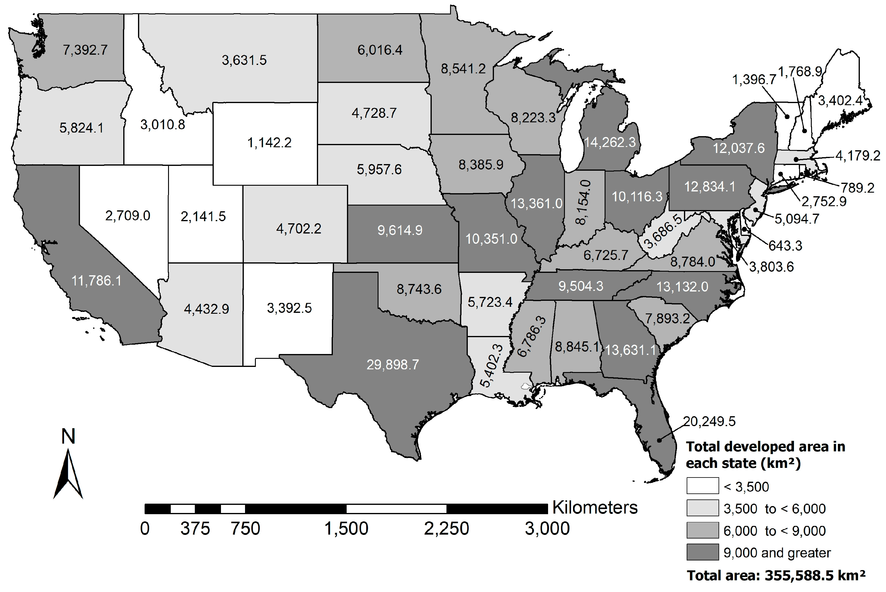
• (1) Damage to climate resulting from loss of land that could be used for potential soil carbon (C) sequestration because of land development within the contiguous USA, with a sum of 355,588.5 km² of land area converted to developments before and including 2016 (Figure 4, Table S6). The largest area losses from developments were found in Texas (29,898.7 km²), Florida (20,249.5 km²), Michigan (14,262.3 km²), and Georgia (13,631.1 km²) (Table S6). In addition, geospatial analysis can determine the amount of temporal change between two points in time. For example, between 2001 and 2016, new developments caused a total of 24,292.2 km² of conversion to developments (Figure S1, Table S7). The largest area losses from development were found in Texas (3888.7 km²), Florida (1676.3 km²), Georgia (1604.6 km²), and North Carolina (1166.7 km²) (Figure S1, Table S7). According to Table 4, there is limited land for nature-based C sequestration, with a total of 34.6% (19.1% shrub/scrub, 15% herbaceous, 0.5% barren land) available. Allocation of land for C sequestration efforts will be limited by projected sea level rise and additional development to accommodate population growth. Loss of land to developments in the contiguous USA is accompanied by GHG emissions and has a long-lasting reduction in C sequestration potential worldwide since CO₂ emissions are of a transnational nature. Variability in area losses to development in various US states illustrates a common issue of inequity in climate change where some states contribute more to GHG emissions and reduction in C sequestration potential because of development than others [23]. Previous research indicated a challenge in quantifying climate change inequity, which can be addressed by using geospatial analysis as demonstrated by this study. Figure 4 demonstrates this spatial inequity, with some states developing larger areas at the expense of current and future C sequestration and other ecosystem service benefits from undeveloped land.

The impact of land developments is not only limited to reduction of C sequestration potential worldwide but also creates local detrimental climate change impacts (e.g., urban heat islands, increased flooding, etc.). Increased impervious surface areas from developments can cause urban heat islands which amplify the impact of climate change on urban environments [24]. Increases in developed areas lead to more impervious areas which are more prone to climate-change-linked flooding [25].

Figure 4. Inequities in damages to climate because of loss of land for potential soil carbon (C) sequestration from developments (before and including 2016) in the contiguous United States of America (USA). Because some of the land development would have preceded the establishment of soil databases, the calculated results for developed areas underestimate their true values.

Figure 4. Inequities in damages to climate because of loss of land for potential soil carbon (C) sequestration from developments (before and including 2016) in the contiguous United States of America (USA). Because some of the land development would have preceded the establishment of soil databases, the calculated results for developed areas underestimate their true values.

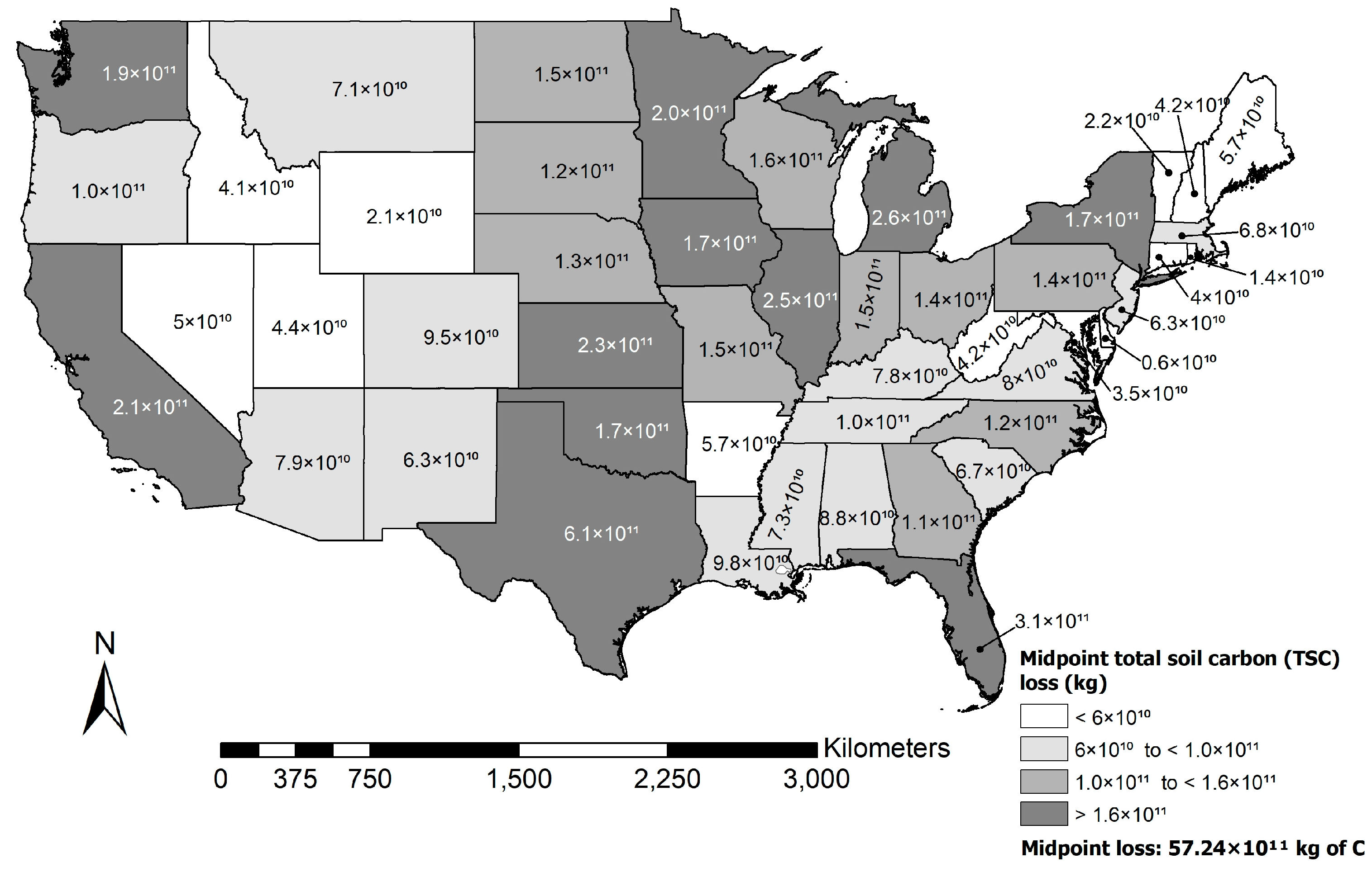
• (2) Damage to climate because of soil carbon (C) loss and associated emissions from land developments in the contiguous USA, with an estimated midpoint total of 57.2 × 10¹¹ kg of C losses (Figure 5, Table S6). The highest soil C losses occurred in Texas (6.1 × 10¹¹ kg C), Florida (3.0 × 10¹¹ kg C), Michigan (2.6 × 10¹¹ kg C), and Illinois (2.5 × 10¹¹ kg C) (Table S6). New development activity between 2001 and 2016 caused a total of 4.1 × 10¹¹ kg in C losses (Table S7, Figure S2). The highest midpoint soil C losses for this more recent time interval occurred in Texas (8.5 × 10¹⁰ kg C), Florida (2.7 × 10¹⁰ kg C), Illinois (1.6 × 10¹⁰ kg C), and Georgia (1.3 × 10¹⁰ kg C) (Table S7, Figure S2).

Variability in TSC loss from various US states illustrates a common issue of inequity in climate change where some states contribute more to GHG emissions than others [23]. Figure 5 demonstrates this spatial inequity, with some states having higher GHG emissions than others. When comparing TSC loss and climate-related disaster costs [26] there is a match between high TSC loss and these costs for the coastal states of Texas and Florida which have experienced high land development and are vulnerable to climate change damages. Given that GHG emissions are unconstrained by state or country boundaries, impacts from these emissions have a global impact, where there is a mismatch and inequity between the highest GHG emitters with limited climate risk and countries with low emissions and high climate vulnerability [23].

Figure 5. Inequities in damages to climate because of soil carbon (C) loss with associated emissions from developments (before and including 2016) in the contiguous United States of America (USA). Because some of the land development would have preceded the establishment of soil databases, the calculated results for soil C losses underestimate their true values.

Figure 5. Inequities in damages to climate because of soil carbon (C) loss with associated emissions from developments (before and including 2016) in the contiguous United States of America (USA). Because some of the land development would have preceded the establishment of soil databases, the calculated results for soil C losses underestimate their true values.

• (3) Damage to climate which can be measured as “realized” social costs of soil carbon (C) (SC-CO₂) released from the land development process before and including 2016 within the contiguous USA with a total midpoint projected value of $969.2B SC-CO₂ (Figure 6). The highest emission costs have occurred in Texas ($102.4B, 11% of total SC-CO₂), Florida ($50.3B, 5%), Michigan ($44.7B, 4.6%), and Illinois ($41.8B, 4.3%) (Figure 6, Table S6). From 2001 to 2016 new developments caused $76.1B in SC-CO₂ (Table S7). The highest costs for this more recent time interval occurred in Texas ($24.1B, 31.6%), Florida ($4.5B, 5.9%), Illinois ($2.7B, 3.5%), and Georgia ($2.2B, 2.9%) (Table S7, Figure S3).

The above estimates are based on a fixed social cost of CO₂ which does not reflect the actual market-based cost of climate-related disasters. Figure 6 shows that the states of Texas and Florida have the highest SC-CO₂ from developments based on the EPA fixed SC-CO₂ value [20]. According to the National and Atmospheric Administration (NOAA), the highest inflation-adjusted cumulative climate disaster market-based costs in less than a 30-year period (1980 to 2019) were reported for Texas (~$250B) and Florida (~$225B) [26]. This highlights the vulnerability of these coastal states to extreme climate and weather events, with Texas seeing the highest number of various types of disasters, and Florida’s disasters being largely from hurricanes [26]. The increase of developments in these climate change disaster-prone states may represent Reverse Climate Change Adaptation (RCCA) when developments are placed in vulnerable areas.

Figure 6. Damage to climate can be measured as “realized” social costs of soil carbon (C) (SC-CO₂) from developments (before and including 2016) in the contiguous United States of America (USA) using an avoided social cost of carbon (SC-CO₂) value of $46 per CO₂ metric ton, applicable until 2025 (2007 U.S. dollars, with an average discount rate of 3% [20]). The map shows inequities in SC-CO₂ distribution. Because some of the land development would have preceded the establishment of soil databases, the calculated results for the projected costs of associated CO₂ emissions underestimate their true values. Note: B = billion = 10⁹.

Figure 6. Damage to climate can be measured as “realized” social costs of soil carbon (C) (SC-CO₂) from developments (before and including 2016) in the contiguous United States of America (USA) using an avoided social cost of carbon (SC-CO₂) value of $46 per CO₂ metric ton, applicable until 2025 (2007 U.S. dollars, with an average discount rate of 3% [20]). The map shows inequities in SC-CO₂ distribution. Because some of the land development would have preceded the establishment of soil databases, the calculated results for the projected costs of associated CO₂ emissions underestimate their true values. Note: B = billion = 10⁹.

Additional information for newly proposed geospatially enabled indicators. Indicators may lack sufficient information to provide pathways to achieve SDG goals. Developments very often occur on different soil types which have different soil properties including soil C content. Additional information for Figure 4 shows that fertile soils had some of the highest area losses to development ((e.g., Alfisols, 22% of the total developed area in the contiguous USA) and Mollisols (21%)). The same soil types contributed almost half to the total TSC losses (Figure 5) and the corresponding social cost of CO₂ (Figure 6). Using fertile soils for urban development at the expense of nature or agriculture may indicate practices that are inconsistent with the concept of sustainable development.

3.4. SDG 15: Life on Land. Protect, Restore, and Promote Sustainable Use of Terrestrial Ecosystems, Sustainably Manage Forests, Combat Desertification, Halt and Reverse Land Degradation and Biodiversity Loss. 15.3 By 2030, Combat Desertification, Restore Degraded Land and Soil, Including Land Affected by Desertification, Drought and Floods, and Strive to Achieve a Land Degradation Neutral World

Current indicator: 15.3.1 Proportion of land that is degraded over total land area. This indicator can be calculated using a baseline of land cover type, soil C, and satellite-based (low resolution) productivity estimates based on vegetation indexes, followed by a change analysis over time to identify possible land degradation [26]. Conversion from pasture/hay to development removes the land area from any productive land use and is a form of land degradation. Specific metrics based on LULC over time could be combined with soil type information to better define and identify degraded land through its loss of productive use. Since the productivity of soils varies widely, leveraging soil spatial databases could greatly improve the evaluation of this indicator. Furthermore, this one general indicator does not address the other much more specific targets associated with this goal (e.g., drought and floods, etc.).

Newly proposed additional geospatially enabled indicators: 1. Baseline proportion of land by LULC class and soil type linked to the soil health continuum status to determine the amount of degraded land (Metric: area; Scale: local, regional, national, global; Measurement frequency: annual). 2. Loss of land from land developments by soil type over time (e.g., per year) (Metric: area; Scale: local, regional, national, global; Measurement frequency: annual). 3. Change in key land cover categories that represent the change in forest and agricultural land use over time (e.g., evergreen forest, deciduous forest, mixed forest, cultivated crops, hay/pasture) (Metric: %, area; Scale: local, regional, national, global; Measurement frequency: annual). 4. Loss of pedodiversity (soil diversity) over time (e.g., per year) from developments (example analysis output Table 5) (Metric: number and type of soils lost, %, area; Scale: local, regional, national, global; Measurement frequency: annual). Important note: These indicators can be represented spatially to identify patterns and hotspots.

Justification: Geospatial and remote sensing analysis in combination with soil databases can determine the baseline proportion of land by LULC class and soil type linked to the soil health continuum status to determine the amount of degraded land (Figure 3, Table 6). It is difficult to define land degradation, given the variety of soil types, climates, and land use/ disturbance history. Soil degradation can be potentially described in terms of soil health status [27]. Mikhailova et al. (2023) [28] proposed measuring and mapping the soil health continuum and its status by LULC class at the landscape level. It should be noted that the analysis results at the country level can mask the variability of land degradation within smaller spatial units (e.g., states) (Figure 3, Table 6). For example, the state of Indiana is more skewed toward LULC classes with lower soil health status (55.1% cultivated crops, 8.0% hay/pasture, 9.8% developed, and 0.1% barren) compared to the overall US soil health continuum (19.6% cultivated crops, 7.6% hay/pasture, 5.8% developed, and 0.5% barren) because of the high proportion of agriculturally productive soils under cultivated cropping (Alfisols and Mollisols). While this baseline is useful for understanding the land degradation status at any one point in time, it is necessary to track changes in LULC classes over time to understand the trajectory of the soil health continuum and land degradation. Land degradation neutrality can only be evaluated through analysis over time.

A geospatial and remote sensing analysis can also be used to measure protection efforts using the change in land covers over time. This analysis could be performed on any spatial scale (e.g., state or region), however, the overall sustainability of land covers at the country scale, provides a direct measure of the stability of key land uses. Table 5 shows that there is potentially limited protection of forest cover with the change in land cover analysis between 2001 and 2016, showing reductions in deciduous (−3.1%) and evergreen (−3.0%) forests. While there was a small increase in mixed forest (0.2%), this positive impact on sustainability was limited (Table 5). The reduction in pasture/hay (−7.9%) and increase in cultivated croplands (+4.0%) indicate further land degradation (Table 5). The increase in developments (ranging from 3.2% to 28.1% depending on the type of development) and in barren land (+0.1) are further indications that there is no halt or reversal in land degradation (Table 5). Land degradation neutrality (LDN) means “that the balance between ongoing land degradation and land restoration has to be zero” [29]. Land degradation neutrality was not observed in the contiguous US between 2001 and 2016. While this is an overall analysis of the country, a similar type of analysis could be conducted at finer spatial scales to help understand local trends. The limitation of relying on country-level analysis and averages, which are often used for SDGs, is that country-level trends can mask local variability, particularly when a country covers a large spatial extent. In the case of the contiguous USA, data for 48 states with a high degree of geographic variability are averaged overall. For example, Table 7 demonstrates this variability in land degradation when examining LULC changes for several states. There is a consistent trend in LULC changes for the contiguous USA and selected states that are likely associated with land degradation (e.g., reduction in hay/pasture, forest land cover types), with an increase in developed land classes. Overall Table 7, shows that there is land degradation over time with no sign of land degradation neutrality. Land degradation neutrality is connected to a loss of productive land and healthy soils [29], while LULC change analysis can be used to represent the soil health continuum as proposed by Mikhailova et al. (2023) [28]. Land degradation is often associated with agricultural land use and desertification while overlooking the impact of urbanization over time on land degradation [30]. However, landscape-scale analysis in various parts of the world has shown that urbanization can cause land degradation [31,32,33].

Table 6. The proportion of land use/land cover (LULC) in 2016 for selected states in the contiguous United States of America (USA).

NLCD Land Cover Classes (LULC), Soil Health Continuum	Soil Health Status	Contiguous USA	Florida	New Jersey	Texas	California	Michigan	Indiana
		Area, 2016 (% from Total Area)
Woody wetlands	Higher	5.1	26.9	18.3	2.7	0.3	22.5	2.2
Shrub/Scrub		19.1	5.1	0.7	40.3	33.5	1.5	0.1
Mixed forest		4.3	0.8	6.0	2.3	2.7	7.8	2.3
Deciduous forest		11.1	0.5	20.6	2.9	0.7	22.2	21.1
Herbaceous		15.0	3.3	0.6	16.4	15.5	2.7	0.7
Evergreen forest		10.4	20.2	4.5	5.5	26.3	5.2	0.3
Emergent herbaceous wetlands		1.5	6.6	4.6	0.8	0.9	1.1	0.3
Hay/Pasture		7.6	13.0	4.8	10.1	0.8	3.1	8.0
Cultivated crops		19.6	7.3	10.3	13.3	10.2	23.8	55.1
Developed, open space		3.3	8.0	13.1	2.8	3.1	4.9	5.5
Developed, medium intensity		0.7	2.3	5.0	0.8	2.0	1.3	1.1
Developed, low intensity		1.6	4.9	9.1	1.5	1.6	3.2	2.8
Developed, high intensity		0.2	0.7	2.0	0.3	0.6	0.5	0.5
Barren land	Lower	0.5	0.5	0.3	0.2	1.9	0.2	0.1

Note: NLCD = National Land Cover Database.

Table 6. The proportion of land use/land cover (LULC) in 2016 for selected states in the contiguous United States of America (USA).

NLCD Land Cover Classes (LULC), Soil Health Continuum	Soil Health Status	Contiguous USA	Florida	New Jersey	Texas	California	Michigan	Indiana
		Area, 2016 (% from Total Area)
Woody wetlands	Higher	5.1	26.9	18.3	2.7	0.3	22.5	2.2
Shrub/Scrub		19.1	5.1	0.7	40.3	33.5	1.5	0.1
Mixed forest		4.3	0.8	6.0	2.3	2.7	7.8	2.3
Deciduous forest		11.1	0.5	20.6	2.9	0.7	22.2	21.1
Herbaceous		15.0	3.3	0.6	16.4	15.5	2.7	0.7
Evergreen forest		10.4	20.2	4.5	5.5	26.3	5.2	0.3
Emergent herbaceous wetlands		1.5	6.6	4.6	0.8	0.9	1.1	0.3
Hay/Pasture		7.6	13.0	4.8	10.1	0.8	3.1	8.0
Cultivated crops		19.6	7.3	10.3	13.3	10.2	23.8	55.1
Developed, open space		3.3	8.0	13.1	2.8	3.1	4.9	5.5
Developed, medium intensity		0.7	2.3	5.0	0.8	2.0	1.3	1.1
Developed, low intensity		1.6	4.9	9.1	1.5	1.6	3.2	2.8
Developed, high intensity		0.2	0.7	2.0	0.3	0.6	0.5	0.5
Barren land	Lower	0.5	0.5	0.3	0.2	1.9	0.2	0.1

Note: NLCD = National Land Cover Database.

Table 7. Change in land use/land cover (LULC) between 2001 and 2016 in the contiguous United States of America (USA) and selected states.

NLCD Land Cover Classes (LULC), Soil Health Continuum	Soil Health Status	Contiguous USA	Florida	New Jersey	Texas	California	Michigan	Indiana
		Change in Area, 2001–2016 (%)
Woody wetlands	Higher	0.2	1.1	0.3	−0.7	0.2	0.5	0.4
Shrub/Scrub		0.1	14.5	−23.4	−2.8	2.0	52.9	63.5
Mixed forest		0.2	−0.6	−0.9	−1.5	−13.6	0.2	1.1
Deciduous forest		−3.1	24.0	−7.4	−6.8	−3.0	−0.8	−0.9
Herbaceous		0.9	5.4	9.5	0.6	10.5	−6.6	7.5
Evergreen forest		−3.0	−5.0	−1.5	0.2	−7.7	−5.7	−0.9
Emergent herbaceous wetlands		−0.6	−8.1	−2.0	−3.3	0.6	−7.7	−0.3
Hay/Pasture		−7.9	−7.6	−15.5	−4.5	−7.3	−5.2	−7.5
Cultivated crops		4.0	0.7	−4.0	6.6	2.4	0.3	0.3
Developed, open space		3.2	2.4	1.5	7.1	1.2	0.3	2.1
Developed, medium intensity		24.6	31.1	12.2	43.9	10.0	9.7	23.6
Developed, low intensity		7.2	9.2	4.4	14.4	3.6	1.9	5.5
Developed, high intensity		28.1	31.5	7.5	40.1	13.2	14.4	25.4
Barren land	Lower	0.1	−0.8	−11.9	−9.9	−0.3	−4.8	12.2

Note: NLCD = National Land Cover Database.

Table 7. Change in land use/land cover (LULC) between 2001 and 2016 in the contiguous United States of America (USA) and selected states.

NLCD Land Cover Classes (LULC), Soil Health Continuum	Soil Health Status	Contiguous USA	Florida	New Jersey	Texas	California	Michigan	Indiana
		Change in Area, 2001–2016 (%)
Woody wetlands	Higher	0.2	1.1	0.3	−0.7	0.2	0.5	0.4
Shrub/Scrub		0.1	14.5	−23.4	−2.8	2.0	52.9	63.5
Mixed forest		0.2	−0.6	−0.9	−1.5	−13.6	0.2	1.1
Deciduous forest		−3.1	24.0	−7.4	−6.8	−3.0	−0.8	−0.9
Herbaceous		0.9	5.4	9.5	0.6	10.5	−6.6	7.5
Evergreen forest		−3.0	−5.0	−1.5	0.2	−7.7	−5.7	−0.9
Emergent herbaceous wetlands		−0.6	−8.1	−2.0	−3.3	0.6	−7.7	−0.3
Hay/Pasture		−7.9	−7.6	−15.5	−4.5	−7.3	−5.2	−7.5
Cultivated crops		4.0	0.7	−4.0	6.6	2.4	0.3	0.3
Developed, open space		3.2	2.4	1.5	7.1	1.2	0.3	2.1
Developed, medium intensity		24.6	31.1	12.2	43.9	10.0	9.7	23.6
Developed, low intensity		7.2	9.2	4.4	14.4	3.6	1.9	5.5
Developed, high intensity		28.1	31.5	7.5	40.1	13.2	14.4	25.4
Barren land	Lower	0.1	−0.8	−11.9	−9.9	−0.3	−4.8	12.2

Note: NLCD = National Land Cover Database.

The diversity of soils (pedodiversity) is a component of biodiversity and can also be evaluated using a similar geospatial analysis. Evaluating the data on pedodiversity change between 2001 and 2016, it can be concluded that all ten soil orders lost areas to development (Table 5). Soil orders are the most general soil classification level and do not represent the many soil series within each soil order impacted by development. Some of these series, which can be linked to unique habitats, may have been endangered or lost to development. A more detailed analysis at a finer spatial scale could quantify these losses.

4. Discussion

4.1. Significance of the Results for Land/Soil-Related Sustainable Development Goals (SDGs)

4.1.1. Benefits and Limitations of Land/Soil-Related Sustainable Development Goals (SDGs) and Current Indicators

Benefits: United Nations (UN) Sustainable Development Goals are categorized as “soft law” or “no law” with non-binding targets, which are used as coordination efforts towards achieving sustainable development by 2030 by 193 countries [34] (Figure 7). Guzman and Meyer (2010) [34] define “soft law as those nonbinding rules or instruments that interpret or inform our understanding of binding legal rules or represent promises that in turn create expectations about future conduct” [34]. There are various reasons to use soft law in the international context, some of which include but are not limited to coordination efforts toward a goal, uncertainty of scientific knowledge, loss avoidance (e.g., lost reputation, etc.), and the necessity to “adjust expectations in the event of changed circumstances” [34,35]. Soft law often involves hortatory (encouraging) instead of legally binding obligations [34]. For example, as part of the UN SDG effort, specific goals (e.g., SDG Goal 13: Take urgent action to combat climate change and its impacts) and targets (e.g., 13.2 Integrate climate change measures into national policies, strategies, and planning) are used as a roadmap to help with voluntary planning processes to develop pledges to address the SDGs [36]. Statistics related to SDG indicators are being measured and reported on a voluntary basis (e.g., Indicator 13.2.2 Total greenhouse gas emissions per year), which may represent a form of disclosure as is commonly seen in corporate reporting [37]. It should be noted that SDG 13 refers to the United Nations (UN) Framework Convention on Climate Change (UNFCCC) (https://unfccc.int/) (accessed on 10 June 2023) [10] as the primary international, intergovernmental forum for negotiating the global response to climate change. The UNFCCC is regarded as hard law with soft law commitments. The US is currently taking some limited climate change actions (https://www.georgetownclimate.org/) (accessed on 10 June 2023) [22], but none of them address soil-based GHG emissions from land conversions.

The implementation method to address SDGs at the national and regional levels is not specified, which provides a wide range of opportunities for countries to develop new or participate in existing initiatives. For example, the concept of soil health is used both in the USA and the European Union (EU) to partially fulfill soil-related SDGs [38,39]. Soil health initiatives, which evolved from the soil quality concept [38,39], are important steps toward sustainable soil management, but they are often focused on farm-scale agriculture, therefore, ignoring other land uses (e.g., urbanization) affecting soil health. Most of the soil health indicators are challenging to use as a tool to evaluate the progress in the realization of SDGs, which often require geospatially-enabled indicators and monitoring (e.g., remote sensing techniques, etc.) at a national scale [18,39]. According to Lehmann et al. (2020) [39], there is a lack of soil-health indicators related to the climate-change functions of soils, such as GHG emissions and C sequestration, which is critical for UN SDG Goal 13: Take urgent action to combat climate change and its impacts.

The land degradation neutrality (LDN) concept is also used to aid with the realization of SDGs (especially SDG Goal 15, described in Table 1) in the global context [40]. Land degradation neutrality is an inspirational target, that focuses on sustaining land productivity, and maintaining ecosystem functions/services in order to provide for contemporary and future generations [27]. To achieve neutrality, there is a need to balance land degradation with land improvement using sustainable land management (SLM) and restoration [27].

The main benefit of SDGs as a soft law that it sets international responsibility [40] for sustainable development. This soft law helps outline international standards for monitoring sustainable development, which can impact national legislatures. Sustainable Development Goals are not the solution to the hard problems (especially the climate change crisis) but they are steps in the right direction of how to engage the international community to develop a global governance strategy for sustainable development [41,42].

Limitations: One of the main limitations of the SDGs is that they are broad in scope and can be overwhelming to conceptualize and implement. Land/soil resources play an important role in many SDGs, but there are currently almost no basic land/soil indicators available. Our research showed that the current indicators listed in the SDGs are not always sufficient to address the goals and targets. For example, for SDG 15, the indicator is “15.3.1 Proportion of land that is degraded over the total land area” (Table 1), which is too general and does not include information on soil types and LULC classes over time that allows evaluation of the land degradation neutrality and trajectory.

Sustainable Development Goals are designed to provide national-level guidance; however, many larger countries contain administrative units as large as other countries, making the use of country-level indicator statistics too ambiguous. When evaluating LULC and soil types on a country basis that covers a large geographic area and a large number of states (e.g., USA, etc.), tabular summaries “mask” (Table 6) the spatial aspects of where change is occurring. In this case, it may be necessary to analyze geospatially-linked information on a state (e.g., Table 6) or even smaller management unit (e.g., county) to be able to understand where change is occurring (hotspots) and what policy changes may be necessary to alter land management to meet SDGs [43]. Looking at only country-level statistics makes it impossible to attribute unsustainable development practices to locations and responsible parties. Given the transnational nature of development drivers (e.g., large-scale transnational land acquisitions, LSLAs), some aspects of SDGs need to be considered beyond the national level [44]. The research on LSLAs points to two contrasting views on sustainable development [44]. Large-scale agricultural production using LSLAs can be viewed as either threatening small-scale farming and SDGs, or positive to SDGs, by enabling modernization and improving production efficiency [44]. These limitations highlight the need for detailed and spatially explicit statistics in SDG analysis.

Unsustainable development has its roots in past land development decisions, which often create a pattern of unsustainable development behavior in the present time, and can influence future unsustainable development [45]. It is often based on outdated laws, and procedures (or a lack of them), which do not factor in climate change impacts (e.g., sea level rise, flooding, etc.) [45]. For example, a geospatial analysis of recent development in the state of Florida (FL) showed development growth around existing urban areas which are often prone to climate change disasters [45]. Past developments caused land/soil degradation and generated an unpaid debt [46] in the form of GHG emissions, generated social costs of emissions (e.g., SC-CO₂) from land/soil disturbance, and created losses of sequestration potential from land development. It is important to quantify these past losses in order to understand the magnitude and geospatial distribution of these losses to avoid unsustainable development in the future. This research demonstrated a method to quantify and map these losses, which can be used in climate change attribution science to address loss and damage (L&D) and other issues (e.g., equity, fairness, justice, etc.) [47,48].

Sustainable Development Goals (SDGs) are not free and come with costs, which are challenging to estimate, but failure to do so may result in the ultimate cost of inaction to humanity—ecocide and the end of the Anthropocene [49,50]. The concept of social costs is increasingly being used to estimate damages associated with GHG emissions (e.g., SC-CO₂), however, these costs are not assessed or recovered by any administrative entity in the USA [20]. This study demonstrated the use of SC-CO₂ with soil C storage and CO₂ emissions from land development in relation to SDG 13: Climate Action. Associating SC-CO₂ with stored soil C gives an estimate of “avoided” SC-CO₂ of emissions (C sequestration) contrasted with “realized” SC-CO₂ of emissions (CO₂ loss) from soil disturbance as a result of land development. Although historically severely degraded, soils in the contiguous US are still a significant source of C (midpoint 1.1 × 10¹⁴ kg of TSC with a midpoint social costs value of $19.3T), which can be released as CO₂ gas upon soil disturbance, (e.g., land developments). Table S5 reports minimum, midpoint, and maximum TSC storage by state and region. The US region with the highest midpoint TSC storage is the Northern Plains ($4.9T) (Table S5). It should be noted that soil and its TSC stocks are a limited resource.

Most land developments in the contiguous USA (before and including 2016) caused a midpoint of $969.1B (where B = billion = 10⁹, USD) in realized social costs of carbon dioxide emissions, SC-CO₂. These SC-CO₂ costs varied by state and region (Figure 6, Table S6), with the Midwest region having the highest midpoint realized SC-CO₂ from “old” developments ($250.3B, Table S6). The “new” land developments between 2001 and 2016 followed the same increasing trajectory, which caused a midpoint of $76.1B in realized SC-CO₂ and also varied by state and region (Table S7). The region with the highest realized SC-CO₂ values was the South Central region ($27.8B, Table S7). It is important to note that the highest realized SC-CO₂ shifted from the Midwest region to the South Central region when considering historical vs. more recent development trends (Tables S6 and S7). The highest SC-CO₂ values for both past and new developments were associated with the states of Texas (TX) and Florida (FL). The existing modus operandi (“business as usual”) for land development appears to internalize profits while externalizing SC-CO₂ costs worldwide [51]. Estimation of these past and recent emissions can be important evidence for climate change attribution science [52]. In addition, there is an inherent conflict between the need for development and sustainability because developments generate economic benefits, revenue, and taxes [53]. Last but not least limitations of the SDGs are that they are not binding and enforceable in the current international legal system, therefore they may be even weaker than soft law and resemble aspirational politics [54].

Indeed, it is possible that SDGs may retard progress on environmental issues such as climate change. The existing literature assumes that agreements on SDGs will promote actual environmental progress [55,56,57]. That is, the assumption is, in economic terms, that SDG is a complement to actual progress: the soft, aspirational SDGs will nudge the world toward the actual achievement of the aspirations [55,56,57].

However, it is probable that, at least in some instances, SDGs, rather than promoting progress, are instead a substitute for progress. Although SDGs usually have wonderful aspirations, they rarely impose specific requirements or mandatory schedules of achievement. The SDGs usually provide no specific timeline for how goals must be achieved; the only certainty is that the goal is to be achieved far in the future. A typical SDG will indicate as a goal some admirable improvement, like reducing GHGs, in the distant future. The politician who agrees to this SDG can then brag to constituents about being a dedicated environmentalist. However, the SDG requires the politician to do exactly nothing. The politician can reap the political benefits of seeming to protect the environment, but without bearing any of the necessary costs of actually achieving anything. For example, the politician need not impose costs on constituents such as by raising taxes, reducing the burning of fossil fuels, or limiting development and soil disturbance. Politicians can claim that they are doing something while doing nothing.

The SDG thus may sometimes retard actual environmental progress. Instead of a leader actually acting now to incur the necessary costs for protecting the environment, the leader attends an international conference of world leaders and agrees to vague, unmeasurable, unenforceable SDGs. The SDGs impress constituents and create the impression of progress. However, the leader then does nothing to achieve the SDG, imposing none of the costs on constituents that would be necessary for actual progress, but that would irritate the constituents. The politician gets political credit for being an environmentalist, but without the additional taxes, higher energy prices, or limits of development that would be necessary for actual progress. The ineffectual hot air of SDGs substitutes for the hard, costly work that actual progress would require. The SDG permits the leader to avoid incurring the political costs that would need to be incurred to improve sustainability and the environment while enjoying the political benefits of seeming to have achieved something.

This paper’s results section demonstrates that our approach would permit the creation of a much more precise SDG, with a precise, measurable final goal and precise, measurable intermediate waypoints for assessing progress toward the goal. But it’s uncertain whether politicians and other leaders would welcome SDGs that are specific and measurable. Such SDGs would render the politicians accountable for achieving the final goals and intermediate waypoints, forcing the politicians to impose the costs that would be necessary for achieving the goals. The real, measurable SDGs that our paper permits would require politicians to impose real sacrifice. Although such SDGs are the only path to real progress, politicians may shun them. Current SDGs tend to be vague aspirations for far in the future, rather than precise goals with precise, measurable timelines for achievement starting immediately. Political support for an SDG may evaporate if, as our results allow, the goal and the timeline of costs for achieving the goal are measured with precision.

So, SDGs may sometimes be a substitute for real progress; they may retard progress, rather than leading it. SDGs permit politicians and leaders to avoid using political capital to make the necessary hard choices about the environment. SDGs permit politicians to establish non-binding inspirational goals while doing nothing. Current SDGs please everybody: environmentalists enjoy the SDGs lofty goals, while those who care little about the environment bear no costs. SDGs may sometimes permit real solutions to environmental problems, with costly solutions, to be ignored.

4.1.2. Refining Land/Soil-Related Sustainable Development Goals (SDGs) and Indicators

Sustainable Development Goals provide an important framework for data collection and analysis enabling future disclosure and accountability as part of sustainable development. The results of these efforts can be used to evaluate the possibility of evolving SDGs from soft law into hard law, especially with regard to climate change [58]. The purpose of such efforts would be to hold states accountable for their past, ongoing conduct and prevent future damages [58].

This study provided examples of using land/soils directly or indirectly in four (Goals 2, 12, 13, and 15) out of 17 SDGs providing recommendations to enhance and expand the current land/soil indicators. Examples were provided using LULC and soil data for the contiguous USA. Technological advances using remote sensing and soil databases (and future soil database development) can be used to standardize the evaluation of SDG implementation worldwide on an ongoing basis (Figure 1), which could help identify opportunities for regional collaboration to address SDGs [59]. There is increasing research in linking satellite data to SDGs using “essential variables” (e.g., land cover, soil moisture, soil C) which include directly and indirectly related variables linked to climate and SDGs [60]. The current spatially explicit systems utilize remote sensing but do not utilize the wealth of information that can be derived from the intersection of LULC change and soil databases [59]. Analysis of the land cover change in urbanizing areas that examines the land consumption rate and population growth rate in relation to SDGs [61] could include soil databases to help prioritize land development that minimizes loss of soil C. The potential of integrating SDGs and ecosystem services [62] can provide cost/benefit analysis to help evaluate progress towards sustainable development.

Soil scientists play an important role in providing expert pedological knowledge on the subject of land/soil SDGs [63,64]. These experts can identify appropriate soil properties and functions to monitor progress toward related SDGs. The selection of soil properties could be expanded beyond typical metrics (e.g., SOC) by including SIC and TSC to avoid underestimation of soil C release across the full range of soil types. In order to assess the progress to meet SDGs, it is necessary to determine a current baseline environmental status. In addition, it may be insightful, where appropriate, to monitor past trends, rates of change, and hotspot locations of indicator values. This analysis can also reveal the drivers behind these variables. If these changes are found to be unsustainable within the SDG framework, there is a need to set binding targets and develop strategies for improvement. In addition, this knowledge could help drive management systems that suggest appropriate land uses aligned with soil and climate capabilities to improve sustainable use [65]. Spatially enabled SDG indicator monitoring, mandatory reporting, and auditing [66] will be needed to disseminate information to decision-makers.

5. Conclusions

This study examined the role that land/soil can play in multiple SDGs (SDG 2: Zero Hunger; SDG 12: Responsible Consumption and Production; SDG 13: Climate Action; SDG 15: Life on Land) and has provided example methods for how geospatial analysis can be used to track relevant qualitative and quantitative land/soil data using the contiguous United States of America (USA) as a case study. Although many currently used SDG targets and indicators are related to land/soil, they do not use land/soil metrics which makes them difficult to evaluate and track. To best support SDGs, land/soil metrics need to be scalable across a variety of spatial and temporal levels. Current indicators for the SDGs of this study have been evaluated, and new additional geospatially enabled indicators have been proposed and justified as enhanced metrics. These enhanced metrics will prove valuable for monitoring past trends and critical areas that may require protection from development, and ultimately for assisting in the attainment of the SDGs. With the ever-expanding sources of remotely sensed imagery and new deep-learning image classification techniques, it is possible to monitor land cover transitions linked to soil-based GHG emissions at detailed spatial scales in near-real time. These types of analysis need to be conducted by independent organizations that can monitor land cover changes on a global scale given the global scope of GHG emissions, instead of focusing on country-level analysis. This would also allow the standardization of spatially enabled indicators across country boundaries while providing equal opportunities to use the latest data sources and processing techniques.

Although land/soil information would be helpful in monitoring progress toward SDGs, political considerations may cause decision-makers not to use the information. An unscrupulous politician benefits from vague, unmeasurable goals extending far into the future because they provide cover for inaction. The improved metrics that this work offers both for establishing specific, detailed SDGs and for measuring progress toward them with precision may be rejected by politicians and other leaders. Sustainable Development Goals may currently be attractive to politicians and leaders precisely because they are soft and vague, and lack specific, measurable timelines for achievement. Current SDGs permit leaders to pose as environmental champions while doing nothing: imposing none of the costs that would be necessary to move forward. So current SDGs may retard progress, permitting leaders to substitute hot air for action. Support for SDGs may evaporate if, as this paper suggests, SDGs and timelines for achievement are made precise and measurable. Agreeing to a vague goal of goodness to be reached decades from now is one thing. Agreeing to goals that will require measurable cost and sacrifice now is another.

References

1. United Nations (UN). Transforming Our World: The 2030 Agenda for Sustainable Development; The Resolution Adopted by the General Assembly on 25 September 2015; United Nations: New York, NY, USA, 2015; 35p. [Google Scholar]
2. United Nations (UN) General Assembly. Global Indicator Framework for the Sustainable Development Goals and Targets of the 2030 Agenda for Sustainable Development; United Nations Statistics Division: New York, NY, USA, 2017; Available online: https://unstats.un.org/sdgs/indicators/indicators-list/ (accessed on 20 June 2023).
3. Keesstra, S.D.; Bouma, J.; Wallinga, J.; Tittonell, P.; Smith, P.; Cerdà, A.; Montanarella, L.; Quinton, J.; Pachepsky, Y.; Van Der Putten, W.H.; et al. Forum paper: The significance of soils and soil science towards realization of the UN sustainable development goals (SDGs). Soil Discuss. 2016, 2, 1–28. [Google Scholar] [CrossRef]
4. Bouma, J.; Montanarella, L.; Evanylo, G. The challenge for the soil science community to contribute to the implementation of the UN Sustainable Development Goals. Soil Use Manag. 2019, 35, 538–546. [Google Scholar] [CrossRef]
5. Hák, T.; Janoušková, S.; Moldan, B. Sustainable Development Goals: A need for relevant indicators. Ecol. Indic. 2016, 60, 565–573. [Google Scholar] [CrossRef]
6. Mikhailova, E.A.; Zurqani, H.A.; Post, C.J.; Schlautman, M.A.; Post, G.C. Soil diversity (pedodiversity) and ecosystem services. Land 2021, 10, 288. [Google Scholar] [CrossRef]
7. Jónsson, J.Ö.G.; Davíðsdóttir, B.; Jónsdóttir, E.M.; Kristinsdóttir, S.M.; Ragnarsdóttir, K.V. Soil indicators for sustainable development: A transdisciplinary approach for indicator development using expert stakeholders. Agric. Ecosyst. Environ. 2016, 232, 179–189. [Google Scholar] [CrossRef]
8. Singh, R.K.; Murty, H.R.; Gupta, S.K.; Dikshit, A.K. An overview of sustainability assessment methodologies. Ecol. Indic. 2012, 15, 281–299. [Google Scholar] [CrossRef]
9. United Nations (UN) General Assembly. Resolution 68/261. Fundamental Principles of Official Statistics. Resolution Adopted by the General Assembly on 29 January 2014. Available online: https://documents-dds-ny.un.org/doc/UNDOC/GEN/N13/455/11/PDF/N1345511.pdf?OpenElement (accessed on 26 July 2023).
10. United Nations (UN) Framework Convention on Climate Change. Available online: https://unfccc.int/ (accessed on 26 July 2023).
11. Brady, N.C.; Weil, R.R. The Nature and Properties of Soils, 13th ed.; Pearson Education Inc.: Upper Saddle River, NJ, USA, 2002; pp. 86–87. [Google Scholar]
12. Soil Survey Staff, Natural Resources Conservation Service, United States Department of Agriculture. n.d.a. Soil Survey Geographic (SSURGO) Database. Available online: https://nrcs.app.box.com/v/soils (accessed on 10 May 2023).
13. The United States Census Bureau. TIGER/Line Boundary Shapefiles. 2018. Available online: https://www.census.gov/geographies/mapping-files/time-series/geo/tiger-line-file.2018.html (accessed on 10 May 2023).
14. Auch, R.F.; Wellington, D.F.; Taylor, J.L.; Stehman, S.V.; Tollerud, H.J.; Brown, J.F.; Loveland, T.R.; Pengra, B.W.; Horton, J.A.; Zhu, Z.; et al. Conterminous United States land-cover change (1985–2016): New insights from annual time series. Land 2022, 11, 298. [Google Scholar] [CrossRef]
15. Multi-Resolution Land Characteristics Consortium—MRLC. Available online: https://www.mrlc.gov/ (accessed on 1 September 2022).
16. Soil Survey Staff, Natural Resources Conservation Service, United States Department of Agriculture. U.S. General Soil Map (STATSGO2). Available online: https://sdmdataaccess.sc.egov.usda.gov (accessed on 23 June 2023).
17. Groshans, G.R.; Mikhailova, E.A.; Post, C.J.; Schlautman, M.A.; Zhang, L. Determining the value of soil inorganic carbon stocks in the contiguous United States based on the avoided social cost of carbon emissions. Resources 2019, 8, 119. [Google Scholar] [CrossRef]
18. United Nations Committee of Experts on Global Geospatial Information Management (UN-GGIM). The SDGs Geospatial Roadmap. Prepared by the Inter-Agency and Expert Group on the Sustainable Development Goals Indicators. Statistical Commission. Fifty-Third Session, 1–4 March 2022. Item 3(a) of the Provisional Agenda Items for Discussion and Decision: Data and Indicators for the 2030 Agenda for Sustainable Development. Available online: https://unstats.un.org/unsd/statcom/53rd-session/documents/BG-3a-SDGs-Geospatial-Roadmap-E.pdf (accessed on 26 July 2023).
19. Guo, Y.; Amundson, R.; Gong, P.; Yu, Q. Quantity and spatial variability of soil carbon in the conterminous United States. Soil Sci. Soc. Am. J. 2006, 70, 590–600. [Google Scholar] [CrossRef]
20. EPA—United States Environmental Protection Agency. The Social Cost of Carbon. EPA Fact Sheet. 2016. Available online: https://19january2017snapshot.epa.gov/climatechange/social-cost-carbon_.html (accessed on 15 September 2022).
21. ESRI (Environmental Systems Research Institute). ArcGIS Pro 2.6. Available online: https://pro.arcgis.com/en/pro-app/2.6/get-started/whats-new-in-arcgis-pro.htm (accessed on 1 March 2023).
22. The Georgetown Law. Georgetown Climate Center. Available online: https://www.georgetownclimate.org/ (accessed on 26 July 2023).
23. Althor, G.; Watson, J.E.; Fuller, R.A. Global mismatch between greenhouse gas emissions and the burden of climate change. Sci. Rep. 2016, 6, 20281. [Google Scholar] [CrossRef]
24. Halder, B.; Bandyopadhyay, J.; Banik, P. Evaluation of the climate change impact on urban heat island based on land surface temperature and geospatial indicators. Int. J. Environ. Res. 2021, 15, 819–835. [Google Scholar] [CrossRef]
25. Ntelekos, A.A.; Oppenheimer, M.; Smith, J.A.; Miller, A.J. Urbanization, climate change and flood policy in the United States. Clim. Chang. 2010, 103, 597–616. [Google Scholar] [CrossRef]
26. National and Atmospheric Administration (NOAA). 2010–2019: A Landmark Decade of U.S. Billion-Dollar Weather and Climate Disasters. 2020. Available online: https://www.climate.gov/news-features/blogs/beyond-data/2010-2019-landmark-decade-us-billion-dollar-weather-and-climate (accessed on 20 August 2023).
27. Mekanizma, U.K. Land Degradation Neutrality Target Setting—A Technical Guide. Draft for Consultation during the Land Degradation Neutrality Target Setting Programme Inception Phase Global Mechanism of the UNCCD, Bonn, Germany, 2016; p. 68. Available online: https://knowledge.unccd.int/sites/default/files/2018-08/LDN%20TS%20Technical%20Guide_Draft_English.pdf (accessed on 10 June 2023).
28. Mikhailova, E.A.; Lin, L.; Hao, Z.; Zurqani, H.A.; Post, C.J.; Schlautman, M.A.; Post, G.C.; Shepherd, G.B.; Dixon, R.M. Quantifying damages to soil health and emissions from land development in the state of Illinois (USA). Land 2023, 12, 1567. [Google Scholar] [CrossRef]
29. Hannam, I. Soil governance and land degradation neutrality. Soil Secur. 2022, 6, 100030. [Google Scholar] [CrossRef]
30. Batunacun; Wieland, R.; Lakes, T.; Yunfeng, H.; Nendel, C. Identifying drivers of land degradation in Xilingol, China, between 1975 and 2015. Land Use Policy 2019, 83, 543–559. [Google Scholar] [CrossRef]
31. Coluzzi, R.; Bianchini, L.; Egidi, G.; Cudlin, P.; Imbrenda, V.; Salvati, L.; Lanfredi, M. Density matters? Settlement expansion and land degradation in peri-urban and rural districts of Italy. Environ. Impact Assess. Rev. 2022, 92, 106703. [Google Scholar] [CrossRef]
32. Bajocco, S.; De Angelis, A.; Perini, L.; Ferrara, A.; Salvati, L. The impact of land use/land cover changes on land degradation dynamics: A Mediterranean case study. Environ. Manag. 2012, 49, 980–989. [Google Scholar] [CrossRef]
33. Imbrenda, V.; Quaranta, G.; Salvia, R.; Egidi, G.; Salvati, L.; Prokopovà, M.; Coluzzi, R.; Lanfredi, M. Land degradation and metropolitan expansion in a peri-urban environment. Geomat. Nat. Hazards Risk 2021, 12, 1797–1818. [Google Scholar] [CrossRef]
34. Guzman, A.; Meyer, T.L. International soft law. J. Leg. Anal. 2010, 2, 171–225. [Google Scholar] [CrossRef]
35. Nadarajah, H. Fewer Treaties, More Soft Law: What Does It Mean for the Arctic and Climate Change. Arctic Yearbook. 2020. Available online: https://arcticyearbook.com/images/yearbook/2020/Scholarly-Papers/15_Nadarajah.pdf (accessed on 10 June 2023).
36. Brus, M.M. Soft Law in Public International Law: A Pragmatic or a Principled Choice? Comparing the Sustainable Development Goals and the Paris Agreement; Springer International Publishing: Cham, Switzerland, 2018; pp. 243–266. [Google Scholar]
37. LoPucki, L.M. Corporate greenhouse gas disclosures. UC Davis Law Rev. 2022, 56, 405. [Google Scholar]
38. Bonfante, A.; Basile, A.; Bouma, J. Targeting the soil quality and soil health concepts when aiming for the United Nations Sustainable Development Goals and the EU Green Deal. Soil 2020, 6, 453–466. [Google Scholar] [CrossRef]
39. Lehmann, J.; Bossio, D.A.; Kögel-Knabner, I.; Rillig, M.C. The concept and future prospects of soil health. Nat. Rev. Earth Environ. 2020, 1, 544–553. [Google Scholar] [CrossRef] [PubMed]
40. Dupuy, P.M. Soft Law and the International Law of the Environment. Mich. J. Int. Law 1990, 12, 420–435. Available online: https://repository.law.umich.edu/mjil/vol12/iss2/4 (accessed on 10 June 2023).
41. Byrnes, R.; Lawrence, P. Can soft law solve hard problems?: Justice, legal form and the Durban-mandated climate negotiations. Univ. Tasman. Law Rev. 2015, 34, 34–67. [Google Scholar]
42. Biermann, F.; Kanie, N.; Kim, R.E. Global governance by goal-setting: The novel approach of the UN Sustainable Development Goals. Curr. Opin. Environ. Sustain. 2017, 26, 26–31. [Google Scholar] [CrossRef]
43. Szabo, S.; Nicholls, R.J.; Neumann, B.; Renaud, F.G.; Matthews, Z.; Sebesvari, Z.; AghaKouchak, A.; Bales, R.; Ruktanonchai, C.W.; Kloos, J.; et al. Making SDGs work for climate change hotspots. Environ. Sci. Policy Sustain. Dev. 2016, 58, 24–33. [Google Scholar] [CrossRef]
44. Dell’Angelo, J.; D’Odorico, P.; Rulli, M.C. Threats to sustainable development posed by land and water grabbing. Curr. Opin. Environ. Sustain. 2017, 26, 120–128. [Google Scholar] [CrossRef]
45. Mikhailova, E.A.; Lin, L.; Hao, Z.; Zurqani, H.A.; Post, C.J.; Schlautman, M.A.; Post, G.C.; Shepherd, G.B.; Kolarik, S.J. Enhancing the definitions of climate-change loss and damage based on land conversion in Florida, USA. Urban Sci. 2023, 7, 40. [Google Scholar] [CrossRef]
46. Sanderman, J.; Hengl, T.; Fiske, G.J. Soil carbon debt of 12,000 years of human land use. Proc. Natl. Acad. Sci. USA 2017, 114, 9575–9580. [Google Scholar] [CrossRef]
47. Mikhailova, E.A.; Lin, L.; Hao, Z.; Zurqani, H.A.; Post, C.J.; Schlautman, M.A.; Post, G.C.; Shepherd, G.B. Delaware’s Climate Action Plan: Omission of source attribution from land conversion emissions. Laws 2022, 11, 41. [Google Scholar] [CrossRef]
48. Menton, M.; Larrea, C.; Latorre, S.; Martinez-Alier, J.; Peck, M.; Temper, L.; Walter, M. Environmental justice and the SDGs: From synergies to gaps and contradictions. Sustain. Sci. 2020, 15, 1621–1636. Available online: https://hdl.handle.net/10779/uos.23476370.v1 (accessed on 10 June 2023). [CrossRef]
49. Vorisek, D.L.; Yu, S. Understanding the Cost of Achieving the Sustainable Development Goals. World Bank Policy Research Working Paper 9164. 2020. Available online: https://documents1.worldbank.org/curated/en/744701582827333101/pdf/Understanding-the-Cost-of-Achieving-the-Sustainable-Development-Goals.pdf (accessed on 10 June 2023).
50. Stock, C. A Fifth core crime: Crime of ecocide as a new puzzle of the international criminal law. Yearb. Int. Eur. Crim. Proced. Law 2023, 1, 248–284. [Google Scholar] [CrossRef]
51. Filippelli, G.M.; Taylor, M.P. Addressing pollution-related global environmental health burdens. GeoHealth 2018, 2, 2–5. [Google Scholar] [CrossRef] [PubMed]
52. Burger, M.; Wentz, J.; Horton, R. The law and science of climate change attribution. Columbia J. Environ. Law 2020, 45, 57. [Google Scholar] [CrossRef]
53. Mikhailova, E.A.; Lin, L.; Hao, Z.; Zurqani, H.A.; Post, C.J.; Schlautman, M.A.; Post, G.C.; Shepherd, G.B. Conflicts of interest and emissions from land conversions: State of New Jersey as a case study. Geographies 2022, 2, 669–690. [Google Scholar] [CrossRef]
54. Duvic-Paoli, L.A. From aspirational politics to soft law?: Exploring the international legal effects of sustainable development Goal 7 on affordable and clean energy. Melbourne J. Int. Law 2021, 22, 1–23. [Google Scholar]
55. Kim, R.E. The nexus between international law and the sustainable development goals. Rev. Eur. Comp. Int. Environ. Law 2016, 25, 15–26. [Google Scholar] [CrossRef]
56. Pavoni, R.; Piselli, D. The sustainable development goals and international environmental law: Normative value and challenges for implementation. Veredas Direito 2016, 13, 13–60. Available online: https://ssrn.com/abstract=2919246 (accessed on 10 June 2023). [CrossRef]
57. Atapattu, S. From our common future to sustainable development goals: Evolution of sustainable development under international law. Wis. Int. Law J. 2018, 36, 215. [Google Scholar]
58. Keenan, P.J. International criminal law and climate change. Boston Univ. Int. Law J. 2019, 37, 89. [Google Scholar]
59. Giuliani, G.; Mazzetti, P.; Santoro, M.; Nativi, S.; Van Bemmelen, J.; Colangeli, G.; Lehmann, A. Knowledge generation using satellite earth observations to support sustainable development goals (SDG): A use case on land degradation. Int. J. Appl. Earth Obs. Geoinf. 2020, 88, 102068. [Google Scholar] [CrossRef]
60. Ballari, D.; Vilches-Blázquez, L.M.; Orellana-Samaniego, M.L.; Salgado-Castillo, F.; Ochoa-Sánchez, A.E.; Graw, V.; Turini, N.; Bendix, J. Satellite Earth observation for essential climate variables supporting Sustainable Development Goals: A review on applications. Remote Sens. 2023, 15, 2716. [Google Scholar] [CrossRef]
61. Song, W.; Cao, S.; Du, M.; Lu, L. Distinctive roles of land-use efficiency in sustainable development goals: An investigation of trade-offs and synergies in China. J. Clean. Prod. 2023, 382, 134889. [Google Scholar] [CrossRef]
62. Yin, C.; Zhao, W.; Ye, J.; Muroki, M.; Pereira, P. Ecosystem carbon sequestration service supports the Sustainable Development Goals progress. J. Environ. Manag. 2023, 330, 117155. [Google Scholar] [CrossRef]
63. Bouma, J. Soil science contributions towards sustainable development goals and their implementation: Linking soil functions with ecosystem services. J. Plant. Nutr. Soil Sci. 2014, 177, 111–120. [Google Scholar] [CrossRef]
64. Bouma, J. Contributing pedological expertise towards achieving the United Nations sustainable development goals. Geoderma 2020, 375, 114508. [Google Scholar] [CrossRef]
65. Liebig, M.A.; Herrick, J.E.; Archer, D.W.; Dobrowolski, J.; Duiker, S.W.; Franzluebbers, A.J.; Hendrickson, J.R.; Mitchell, R.; Mohamed, A.; Russell, J.; et al. Aligning land use with land potential: The role of integrated agriculture. Agric. Environ. Lett. 2017, 2, 170007. [Google Scholar] [CrossRef]
66. Sari, D.A.; Margules, C.; Lim, H.S.; Sayer, J.A.; Boedhihartono, A.K.; Macgregor, C.J.; Dale, A.P.; Poon, E. Performance auditing to assess the implementation of the Sustainable Development Goals (SDGs) in Indonesia. Sustainability 2022, 14, 12772. [Google Scholar] [CrossRef]
Figure 3. Land cover map of the contiguous United States of America (USA) for 2016 (based on data from MRLC [15]).
Land 12 01853 g003
Figure 7. The spectrum between soft and hard law (adapted from Nadarajah (2020) [35]).
Land 12 01853 g007