Abstract
Nowadays, climate change not only leads to riverine floods and flash floods but also to inland excess water (IEW) inundations and drought due to extreme hydrological processes. The Carpathian Basin is extremely affected by fast-changing weather conditions during the year. IEW (sometimes referred to as water logging) is formed when, due to limited runoff, infiltration, and evaporation, surplus water remains on the surface or in places where groundwater flowing to lower areas appears on the surface by leaking through porous soil. In this study, eight different machine learning approaches were applied to derive IEW inundations on three different dates in 2021 (23 February, 7 March, 20 March). Index-based approaches are simple and provide relatively good results, but they need to be adapted to specific circumstances for each area and date. With an overall accuracy of 0.98, a Kappa of 0.65, and a QADI score of 0.020, the deep learning method Convolutional Neural Network (CNN) gave the best results, compared to the more traditional machine learning approaches Maximum Likelihood (ML), Random Forest (RF), Support Vector Machine (SVM) and artificial neural network (ANN) that were evaluated. The CNN-based IEW maps can be used in operational inland excess water control by water management authorities.
1. Introduction
One of the main and permanent challenges of Carpathian Basin water management and the paradoxical hydrological situation is the consecutive occurrence of inland excess water (IEW) and drought at the same locations within years or even seasons.
The description and research into this phenomenon, which is the result of natural and anthropogenic processes, has a long history in domestic water management in Hungary. The definition of the term has constantly been changing in scientific literature, and to date, there is no single definition that can be considered exact [1]. Pálfai has collected over fifty definitions of IEW, thus highlighting the complexity of the phenomenon [2]. He brought the different interpretations together in the following formulation: “IEW is a specific type of water, a periodic but fairly permanent phenomenon in flat areas, covering a relatively large area”. Lászlóffy categorized IEW as all water that is produced from precipitation or groundwater in an area protected by embankments, and that has no natural outlet [3]. According to Rakonczai, “floodwaters generated in flat areas, mostly outside the exempted floodplains of rivers” are called IEW [4]. A distinction can be made between three technical definitions of IEW when inland floods occur: the area is covered by continuous water surfaces, slow water movement accumulates on the ground, and rising water levels in drainage systems [4,5,6]. According to the biological interpretation, IEW is formed “when there is more moisture in the pores in the soil layer than the vegetation can tolerate” [7]. From an economic point of view, “IEW is said to occur when damage is caused when the loss of yield due to flooding or soil saturation exceeds the value of the surplus yield of areas not affected by IEW” [4]. Crop losses are most at risk from IEW in the spring-summer period. Summer IEW is mostly caused by short periods of high-intensity or prolonged low-intensity rainfall, generating yield losses and economic damage [8].
Outside of the Carpathian basin, the phenomenon is also known, e.g., in other low-lying countries like the Netherlands, Poland, and Germany [9]. In other countries, these floods are often referred to as waterlogging [10] or ponding water [11]. Waterlogging is defined as the disruption of the water and oxygen balance in the soil when the root zone of a crop in a waterlogged soil is deprived of oxygen (hypoxia) and the chlorophyll content of the plant is reduced due to stress [10,12,13]. Compared to IEW, this is the process when the open water surface does not yet appear in remotely sensed data, but the plants show signs of stress even in the almost saturated soils. Such studies are commonly observed in irrigated agricultural areas, where soils are saturated with water, and damaging salt accumulations occur [14,15,16,17]. Pounding water is defined as water accumulating in closed depressions. This definition best approximates IEW [11]. Climate change models predict increased precipitation intensity in the Carpathian Basin, which potentially increases the risk of IEW in the future [18]. To effectively address the inundations and take measures to prevent them or mitigate their damage, it is important to understand where and why these natural hazards occur. The inundations can be very dynamic in nature. Depending on meteorological conditions (temperature, precipitation, wind speed) before, during, and after their development, they can quickly appear but also can disappear fast.
Significant advances have been made in the field of IEW research in recent years, which partly address the challenges listed above. With advances in remote sensing and geospatial information technology, synthetic mapping techniques have become increasingly sophisticated. As Awange et al. [19] have formulated, the essence of geospatial modeling is to combine different map layers selected for analysis in such a way as to obtain a new synthetic map layer that, based on the information of the original map layers, provides the user with completely new information. Bozán et al. [20] distinguished three main technical approaches to mapping IEW. Direct mapping is based on the geospatial processing of satellite imagery or aerial photographs. In this case, we see a snapshot of the current situation of the area under study and do not get information on the root causes. Synthetic mapping based on regression of dependent and independent factors allows for the analysis of cause-and-effect relationships but depends heavily on the quality of the databases used [21]. Spanoudaki et al. [22] formulated that there are several model frameworks available for the analysis of hydrological processes and their interpretation (e.g., MIKE SHE [23], MODFLOW [24]). Physics-based models are highly data-intensive and require reliable data sources. Therefore, the measurement and determination of IEW extent by field and/or remote sensing at the national scale is still subject to considerable uncertainty [25,26]. A third approach is integrated hydrological modeling based on the relationship between hydrological variables and IEW discharge. This type of dynamic modeling provides the most detailed information for estimating discharges [27].
To better understand IEW as a natural phenomenon but influenced by anthropogenic factors, it is necessary to follow the evolutionary process of its formation and disappearance. Therefore, studies over longer time series, with a high temporal resolution and over large areas, are required. Satellites can provide data for these studies, but it is essential to use as many of the available images as possible, even if they are partly cloudy. From a water management perspective, it is important to know the extent and duration of IEW inundations, especially in agricultural areas. In the presented work, we investigated which water surface delineation approach based on segmentation, supervised classification, and machine learning is the most effective procedure for creating IEW maps and studying inundation time series. For this purpose, we used multiple Sentinel-2 images with varying degrees of cloud cover. Continuous monitoring can also be used to understand the development of IEW, to mitigate the risk they pose to infrastructure and agriculture, and to understand how surplus water can be reused in periods of drought. We tested threshold-based segmentation of Normalized Difference Vegetation Index (NDVI), Normalized Difference Water Index (NDWI), and Modified Normalized Difference Vegetation Index (MNDWI) maps. We applied supervised classification using the more traditional machine learning models Maximum Likelihood (ML), Random Forest (RF), and Support Vector Machine (SVM). Finally, we applied an artificial neural network (ANN) and Convolutional Neural Network (CNN) to delineate IEW.
NDVI is a well-known, simple index for quantifying green vegetation. The index ranges between −1 and 1. The higher the value, the higher the chlorophyll content of the plants due to the sensitivity differences in the red and near-infrared bands. Lower values are useful for delimiting soil and water surfaces [28,29]. NDVI is one of the most popular indexes used in remote sensing studies [30]. NDWI was first proposed by McFeeters (1996) [31]. It uses the green and near-infrared bands of multispectral data. It is based on the principle that water bodies produce maximum reflection in the green band while showing minimum reflection in the NIR band. The MNDWI method was also used to extract water bodies; it is based on the normalized difference of the green and shortwave infrared bands [32]. Spectral indexes can be sensitive in built-up areas where reflectance from buildings can cause overestimated results [33].
Random forests are a common method for generating land cover classifications [34]. The classification consists of a combination of tree classes, where each tree class is generated using a random vector taken independently from the input. From the vector, and for each tree, the most popular class casts a vote for input classification and vector classification. RF uses a combination of the features of each class in the sample set to select the most popular voted class from all the tree predictors using the trees in the forest [35]. Random forests have been applied in many remote sensing applications [36], including wetland classification [37]. The Support Vector Machine uses a special type of function called “hyperplane” to divide the learning examples into two parts [38]. Such a function specifies to what extent an element belongs to a given class. If there are multiple classes, then multiple functions can be used to implement the classification. A comprehensive overview of the application of SVM and RF in remote sensing is given by Sheykhmousa et al. [39]. Maximum likelihood is a statistical estimation that is used to estimate the parameters of an assumed probability distribution based on some observed data. This is achieved by maximizing a likelihood function such that the set of observed data is the most likely given the hypothesized statistical model. The point in the parameter space that maximizes the likelihood function is called the maximum likelihood estimate. The logic of ML is both intuitive and flexible, and as such, the method has become a dominant tool for statistical inference [40]. The ML algorithm is implemented in many software packages for image processing and is often used as a conventional and robust baseline for classification studies [41,42,43].
Deep learning is a group of machine learning models that represent data at different levels of abstraction by means of multiple processing layers [44]. The simplest version of deep learning is a multi-layer perceptron (MLP) with a large number of hidden layers. MLP is a fully connected artificial neural network in which the parameters are updated in the training phase using the backpropagation algorithm [45]. ANNs have been successfully deployed to many geographic applications, for example, in satellite image classification [46,47] and landslide risk [48]. A special type of deep learning model is the convolutional neural network which was originally designed for computer vision problems. CNNs consist of a series of processing layers, where each layer is a set of convolution filters that detect image features. The early layers form feature detectors that are specialized to detect basic shapes like linear features, corners, or circles, while successive layers form higher-level feature detectors [49]. CNNs have been used in object detection and classification applications ranging from medical imaging to automated driving and remote sensing [50]. In remote sensing applications, the networks have, for example, been used for land use classification based on Sentinel-2 imagery [51], water segmentation [52], and human settlements mapping [53].
The aim of this study is to evaluate eight different machine learning approaches to derive IEW inundations from high-resolution Sentinel-2 imagery on three different dates in 2021. The first date was used to collect the training data, which was then applied to classify each acquisition. A detailed accuracy assessment was conducted to identify the most successful classification method.
2. Materials and Methods
2.1. Study Area
Our research is focused on one of the most vulnerable areas to IEW of the Carpathian Basin (Figure 1). The high clay content of the soil types, the many former buried riverbeds, and the lack of drainage makes this an area highly exposed to inundations. In terms of precipitation, the annual amount of 500–550 mm is not outstanding, but the intra-annual distribution is significant in late winter and early spring (up to 30–50% of the annual precipitation), which may result in the appearance of IEW due to the poor infiltration coefficient of the soils. The area is within the T34TDT tile of the Sentinel-2 satellite. Sentinel-2 is a constellation of two equal multispectral imaging satellites that provide optical data collected in thirteen spectral bands ranging from visible to shortwave infrared at different spatial resolutions from 10 m to 60 m [54]. In this research, 10 bands with a spatial resolution of 10 and 20 m were used. Data are collected from the study area at an average interval of three days. In our comparison, cloud-free images were acquired during the 2021 IEW period on 23 February 2021 and 7 March 2021, while a cloudy image was acquired on 20 March 2021.
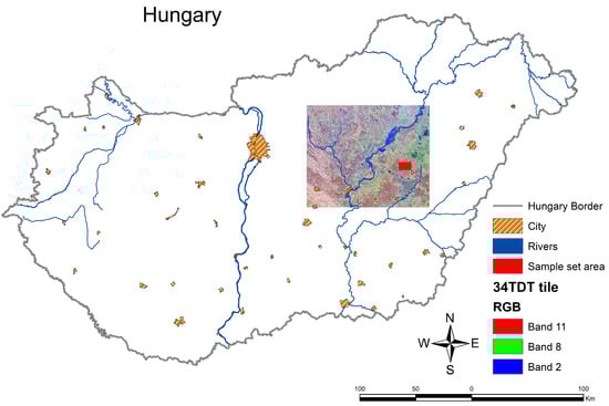
Figure 1.
The Sentinel-2 false-color composite (B11, B8, B2) of 23.02.2021, showing the 34TDT tile and the location of the study area.
2.2. Methodology
A complex methodology has been developed to derive temporary water bodies from Sentinel-2 multispectral high-resolution satellite data (Figure 2). Before applying the methods for the delineation of temporary water bodies, a preprocessing workflow was executed on each satellite image. All spectral bands were converted to a common resolution, resulting in a composite image with a spatial resolution of 10 m. In addition, the Scene Classification Layer (SCL), which is created by the data provider and is included with the image, was used to filter out most of the atmospheric disturbances. The SCL map was used to exclude areas covered by clouds and cloud shadows (classes 3, 8, 9, and 10). Permanent water surfaces, like fishponds, fishing lakes, spas, and thermal baths were also excluded from the study area by visual interpretation and digitizing (Figure 3).
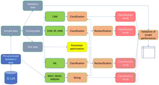
Figure 2.
Workflow for the evaluation of the optimal methodology for water delineation.
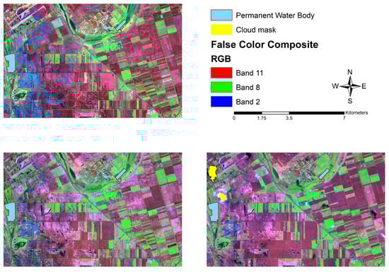
Figure 3.
Sentinel-2 false-color composite of the study area with permanent water bodies and cloud masks at three dates (23 February 2021 (upper left); 7 March 2021 (lower left); and 20 March 2021 (lower right)).
For each acquisition date, NDVI, NDWI, and MNDWI images were calculated using the following equations:
where Green, Red, NIR, and SWIR are, respectively, bands 3, 4, 8, and 11 of Sentinel-2.
The spatial resolution of the SWIR bands is 20 m, which requires a solution for the discrepancy between the resolution of the green and SWIR bands. One possibility would be to produce a 20 m resolution MNDWI by simply aggregating the green band from 10 m to 20 m, but for the sake of uniformity and more accurate delineation of water bodies, we decided to produce a 10 m resolution MNDWI by downscaling the SWIR band from 20 m to 10 m.
Threshold-based segmentation of NDVI, NDWI, and MNDWI was used to create binary (water–no water) maps. A threshold specifies the boundary between water and no water within the specific image. The water thresholds were determined visually on the first image (23 February 2021); NDVI: below 0.17; NDWI: above −0.31; MNDWI: above −0.36. To ensure minimum user intervention, for each acquisition date, the same threshold was used.
ML, RF, and SVM classification methods were used to create thematic maps with nine classes. The classes included the desired water class and other land cover classes. Some classes had a light and dark version when they were covered by cloud shadows. This “dark” class approach aims to improve the classification result. The thematic maps were reclassified to binary water maps to make them comparable with the index-based results. Geoinformatics software ArcGIS Pro 2.9.1 was used to classify the images using ML. The standard parameters were used to run the tool, meaning that all classes had the same a priori probability, and the reject fraction was set to 0, resulting in the classification of all pixels.
The sklearn python package [55] was used to apply the RF and SVM machine learning methods (available as Supplementary Materials Codes S1 and S2). For each method, the data was split into a training (80%) and a validation set (20%). Then the data was standardized by removing the mean and scaling to unit variance. For each of the classification methods, multiple parameters were tested using the grid search function of sklearn with 10-fold cross-validation. For the random forest classifier, the optimal result was reached with 200 trees and a maximum depth of 20. The Radial Basis Function was used for the Support Vector Machine method.
The third group of algorithms that we applied to extract shallow water bodies is the artificial neural network-based models. Two approaches were evaluated. The first approach was a fully connected artificial neural network that was fed with the same training set as was used with ML, RF, and SVM. The artificial neural network is a TensorFlow deep network implementation with 3 dense layers, with resp 16, 12, and 9 neurons, and 20% dropout layers after the first two dense layers (available as Supplementary Material Code S3). The first two layers use ReLu activation, while the last layer uses a softmax activation function. The learning rate of the Adam optimizer was set to 0.004. Also, for the ANN, we used grid search to optimize the hyperparameters. The optimum batch size was 32 with 30 epochs. The ANN resulted in a thematic map with nine classes that were reclassified to a binary water map. The second approach is a convolution neural network that was trained with a large number of examples of known permanent water bodies (Figure 4).
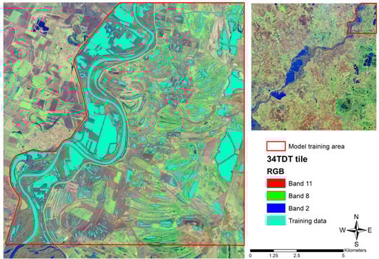
Figure 4.
CNN Model training data with the original Sentinel-2 color composite (upper right) and the digitized permanent water polygons (left).
The polygons were digitized based on visual inspection of the satellite image of the first acquisition date. The trained model was used to classify the images of each date to a binary water map. The deep learning functionality of ArcGIS Pro was used to classify the images with a convolutional neural network. ArcGIS Pro provides a user-friendly interface to deep-learning python libraries like Keras, TensorFlow [56,57], PyTorch [58], and Fastai [59]. The interface enables the specification of most but not all hyperparameters that are available in the libraries. The samples of the IEW patches were used to create 4794 chips of 32 × 32 pixels with an overlap of 16 pixels. Data augmentation was not applied. The labels had two categories: water and no water. The training data was used to train a U-net model [60] with the PyTorch implementation. We used a variable learning rate ranging from 6.3 × 10⁻⁶ to 6.3 × 10⁻⁵, and the number of epochs was maximized to 30 with a batch size of 4. Resnet-34 was applied as a backbone model, where only the weights of the fully connected tail of the model were retrained. After 23 epochs, the training reached its optimum. Experiments with many other combinations of hyperparameters were carried out, but they did not give better training results.
2.3. Validation
The validation of the classification methods was based on independent validation data sets that were manually digitized from the satellite images of the three acquisition date, and they did not overlap with the training samples (Figure 5). The reference polygons were converted to pixels with the same resolution as the model results, and error matrices were produced for each method and acquisition date. The validation metrics are overall user and producer accuracy, Kappa, and QADI [61].
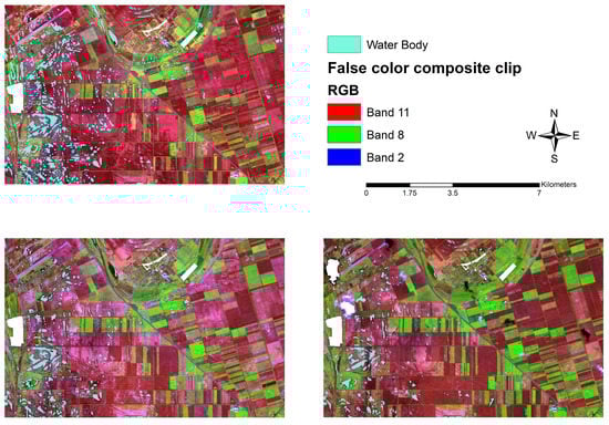
Figure 5.
Manually digitized validation water polygons on the satellite images of the three dates (23 February 2021 (upper left); 7 March 2021 (lower left); 20 March 2021 (lower right)).
3. Results
Eight different methods were applied to classify Sentinel-2 images of three different dates. For each method, an accuracy matrix was calculated, and metrics were derived to assess the quality of the classification. The classifications are shown on the result maps (Figure 6, Figure 7, Figure 8, Figure 9, Figure 10, Figure 11, Figure 12, Figure 13, Figure 14, Figure 15 and Figure 16) and tables (Table 1, Table 2, Table 3 and Table 4) using the following categories:
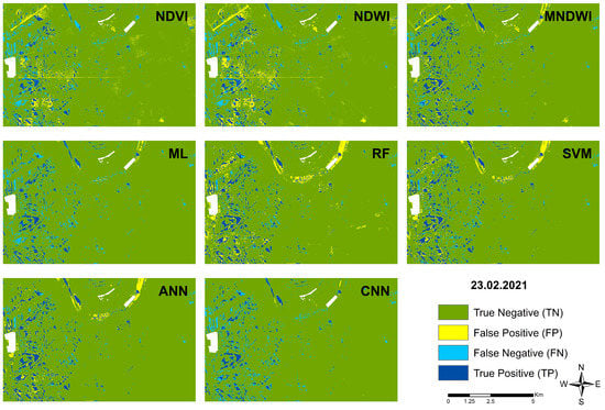
Figure 6.
Results of the different classifications on 23 February 2021.
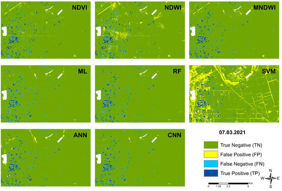
Figure 7.
Results of the different classifications on 7 March 2021.
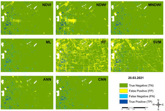
Figure 8.
Results of the different classification on 20 March 2021.
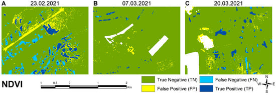
Figure 9.
Examples of classification errors of the NDVI model on different dates, including (A) runway of the airport 23 February 2021; (B) scattered buildings and roads. The white areas are the masked-out permanent water bodies 7 March 2021; and (C) errors due to cloud/shadow mask, 20 March 2021.
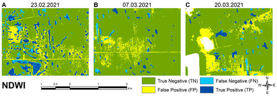
Figure 10.
Examples of NDWI model classification errors at different times. (A) scattered buildings and roads 23 February 2021; (B) bare soils adjacent to roads 7 March 2021; and (C) strong errors near the cloud and shadow mask 20 March 2021.
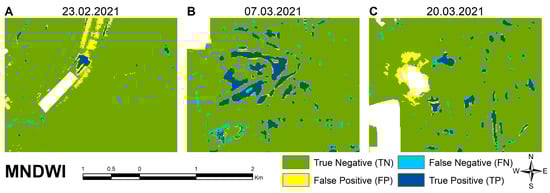
Figure 11.
Examples of MNDWI model classification errors at different times, including (A) Omission in reference map 23 February 2021; (B) shallow water 7 March 2021; and (C) errors near the cloud and shadow mask 20 March 2021.
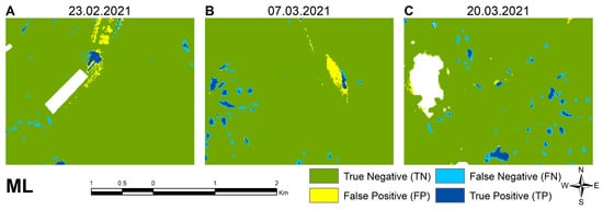
Figure 12.
Examples of maximum likelihood model classification errors at different times, including (A) Omission in reference map 23 February 2021; (B) shallow water 7 March 2021; and (C) cloud and shadow mask and shallow water 20 March 2021.
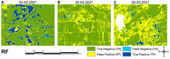
Figure 13.
Examples of random forest model classification errors at different times, including (A) Relatively small omissions 23 February 2021; (B) extreme overclassification in general 20 March 2021; and (C) Extreme overclassification around the cloud and shadow mask 20 March 2021.
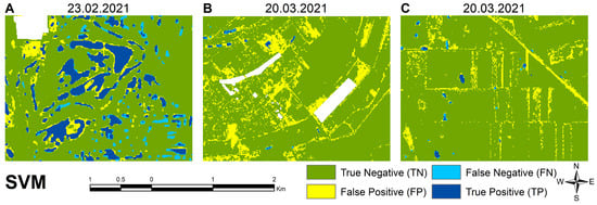
Figure 14.
Examples of support-vector machine model classification errors at different times, including (A) Relatively small omissions 23 February 2021; (B) extreme overclassification 20 March 2021; (C) extreme overclassification 20 March 2021.
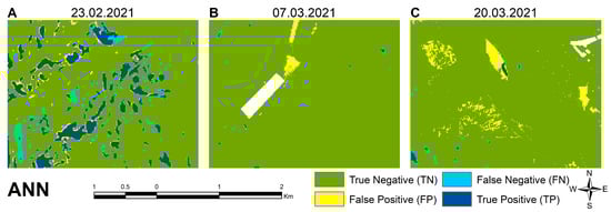
Figure 15.
Examples of artificial neural network model classification errors at different times, including (A) Relatively small omissions 23 February 2021; (B) some overclassification 20 March 2021; and (C) some overclassification due to atmospheric disturbances 20 March 2021.
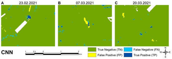
Figure 16.
Examples of convolutional neural network model classification errors at different times, including (A) Omissions of water detection 23 February 2021; (B) some overclassification 7 March 2021; and (C) some overclassification and minor omissions 20 March 2021.

Table 1.
Statistical comparison of methods for the first acquisition date.
Table 2.
Statistical comparison of methods for the second date.
Table 3.
Statistical comparison of methods for the third acquisition dates.
Table 4.
Aggregated results of the accuracy assessment.
- TN (True Negative–dark green): areas where no water was identified on the reference map and the model-generated map;
- TP (True Positive–dark blue): where water has been identified on the reference map and by the model;
- FP (False Positive–yellow): where no water was identified in the reference map, but the model identified water:
- FN (False Negative–light blue): where water was identified in the reference map but not by the model.
We will first present the results of each classification method per acquisition date, followed by a detailed analysis of the problematic areas per method.
3.1. Results of the Total Study Area
Figure 6 shows the result water maps of the first acquisition date. The first row shows the approaches based on the segmentation of index maps using thresholds. As expected, NDVI presented a mixed result since the thresholds were selected based on the index values of the first date. It is clear that the deeper water patches in the validation area are well-defined. These are the true positives. The shallower water patches are not always correctly delineated, and therefore, the number of false negative values (FN, light blue) is nearly equal to the correctly extracted water pixels. The NDWI classification is very similar to the NDVI classification. The properly classified water and non-water pixels are almost the same for the two methods. However, the NDWI method is more sensitive to the built-up environment, with bare soils appearing as false positives. Among the index-based methods, the MNDWI index performed best, especially on the first acquisition date. The number of true positives is much higher than false negatives, which means that shallower water surfaces are better delineated. The second row shows the results of the traditional machine learning models. The ML classification shows good agreement with the validation data. There are quite a lot of missing waterbodies though. Presumably the classification has not been able to perfectly delineate shallow inundations. The RF method detects the water patches quite well, but with some overclassification of water in the northern part of the area. The SVM performed similarly to RF. The hyperplane classification performed relatively well, with well-defined water pixel values and false positives appearing in close proximity to IEW. The third row gives the results of the deep learning models. For the ANN network, we used the same sample set as for the traditional machine learning models (ML, RF, SVM). In general, this model does not misclassify many water bodies, also not in built-in areas, as has been shown in the other methods. The false negative rate is almost the lowest here compared to the other models. The CNN model result for the first date shows that the water bodies are correctly classified but that quite a few inundations are omitted, resulting in a high number of false negatives.
On the second date, MNDWI also performs better than the other two indices (NDVI, NDWI), but the built-up environment (roads, buildings) continues to be misclassified as water surfaces (Figure 7). The ML model still performs well, and the RF model worked surprisingly well compared to the first date. The delineation of water surfaces has improved greatly as both FN and FP almost completely disappeared. The SVM model became completely unstable, and as with the NDVI and NDWI indices, the built-up environment (road, buildings) was identified as a water surface. The deep learning models achieved similarly good results as on the first date.
In the third image, large atmospheric disturbances (clouds, cloud shadows) occur, so it is important to investigate how the models respond to cloud masking and atmospheric interference (Figure 8). The indices performed poorly compared to the first two dates, especially NDWI, where misidentified water surfaces appear abundantly, especially around the cloud masks and on bare soil. For the traditional machine learning models, the RF and SVM classifications have become completely unstable, and many misidentified water surfaces appear in the study area. ML performed well with hardly any false positives. Among deep learning models, ANN is only minimally sensitive to atmospheric disturbances. CNN is not at all sensitive.
3.2. Detailed Analyis of Classiciation Methods
On the first date (23 February 2021), it is clearly visible that the NDVI approach properly delineated the deeper water patches in the validation area. These are the true positives in Figure 9A. The shallower water patches are often omitted, and therefore, the number of false negative values is nearly equal to the correctly extracted water pixels. The sensitivity of the index to low pixel values is shown by the incorrect identification of the runway of the former Kunmadaras airport in the north-western area as water (Figure 9A), as well as the misclassification of other linear facilities (roads) and built-up areas (Figure 9B). Note that the white areas are masked-out permanent water bodies. Increasing the threshold value to include more IEW patches was not possible because this also increased the number of false positive pixels, as can be seen on the first acquisition date. The pixels misidentified as water surfaces also occur next to the cloud mask, which shows the sensitivity of the index to atmospheric disturbances (Figure 9C).
The results for the NDWI classification are very similar to the NDVI classification on the first date (Figure 6). The properly classified water and non-water pixels are almost the same for the two methods. However, the NDWI method is more sensitive to the built-up environment, with bare soils appearing as false positives. They are noticeable near water spots and linear features (Figure 10A). On the second date, besides the increase of properly delineated (deep) water pixels, a lot of pixels were incorrectly identified: built-up areas and bare soils have often been classified as water (Figure 10B). On the date with atmospheric disturbances, extreme overestimation of the water bodies occurred in areas with bare soils and around the masked-out clouds (Figure 10C).
Among the index-based methods, for the total validation area, the MNDWI index performed best, especially on the first acquisition date (Figure 6). A larger misclassified patch is visible in the northern area (Figure 11A), which may be due to errors in the reference map or an imperfectly chosen threshold. On the second date, some minor overclassification of water happened in the immediate vicinity of the water surfaces, which can also be attributed to the aforementioned causes (Figure 11B). The number of true positives is high, and the number of false negatives value is low. This confirms the accuracy of the chosen threshold. On the third date, overall, the results improved further with a small number of false negatives due to missed shallow water. False positives appear in places other than for NDVI and NDWI, for example, near the cloud mask (Figure 11C).
The detailed analysis of the ML classification of the first date shows good agreement with the validation data, although there are quite some shallow inundations missed. There are some false positives only in the northern areas (Figure 12A). On the second date, there are more properly classified water pixels, while only some linear patches in the north, which may have been omitted from the validation data set. False negatives occur around disappearing IEW patches (Figure 12B). Similarly, the third image shows a good match for the water patches but lacks detection of shallower water around the deeper patches. Contrary to the index-based methods, the areas around clouds are not misclassified as water by maximum likelihood (Figure 12C). Considering that the training sample set is constructed based on the first acquisition date, the model performs consistently well on all three dates and is not at all sensitive to the built-up environment, as were the indexes.
The RF method detects the water patches quite well on the first two dates but with extreme overclassification of water on the last date. On the first date, the method detects almost all water, although it can be noted that the delineation of shallow inundation was not perfect during the training (Figure 13A). On the second date, RF performed very well, with almost no false positives. Figure 13B shows that on the last date, the model became completely unstable. The number of false positives is very high, and they are found almost everywhere in the image, as surfaces such as the built-up environment (roads, dirt roads, buildings) and bare soils. Areas around the cloud mask are also misclassified as water (Figure 13C).
The detailed analysis of the SVM shows the same behavior as for RF. On the first date, SVM shows well-defined water pixel values and false positives appearing in close proximity to inland excess water (Figure 14A). On the second and third dates, the proximity of the classes interfered with the positive delineation of the water surfaces, resulting in a very high number of false positives. Similar to the result of the RF model for the image with atmospheric disturbances, built-up areas (Figure 14B) and almost the entire road network were classified as water surfaces (Figure 14C).
On the first date, most of the water was properly identified by the ANN model, although this method shows some false negatives for shallow inundations adjacent to deeper water (Figure 15A). On the second date, a small number of false negatives appeared next to a large number of properly detected water pixels. The model shows good performance, although some misclassification occurred in the northern areas (Figure 15B). In the third image, water pixels continue to be detected well, but due to atmospheric disturbances, thin clouds or cloud shadows were mixed up as water in patches in the central part of the image (Figure 15C).
As with the other methods, the CNN model has difficulties with delineating shallow inundation resulting in scattered false negatives distributed equally over the total validation area. However, the number of false positives is limited to a small section in the northern area (Figure 16A). On the second date, IEW patches are detected, although the shallow water at their boundaries is missing in the classification result. Similar to the ANN result, a large patch in the northern part of the area is wrongly detected, probably due to an error in the validation data (Figure 16B). On the last date, almost all individual IEW patches are properly detected, with some omissions along their borders. The model is insensitive to atmospheric disturbances due to clouds and shadows. Also, their boundaries show only some minimal anomalies (Figure 16C).
3.3. Validation Results
When comparing the methods, we used several accuracy metrics to select the best classification approach. In terms of overall accuracy, we found that due to the asymmetrical class distribution (high number of non-water pixels), each method performs well above 90% in almost all cases. Consequently, we added other metrics, such as the widely used Kappa index (K) and the QADI index (QADI), that are less sensitive to class asymmetry [61], and Sensitivity (S) and Precision (P) [62] (Table 1, Table 2 and Table 3).
where:
P0 is the relative observed agreement among the classification result and the reference, and Pe is the hypothetical probability of chance agreement.
where:
A is the degree of disagreement between the classification result and the reference, and Q quantifies the difference in the pixel count for each class between the classified map and reference data. QADI ranges between 0 and 1, where values below 0.1 are considered good accuracy and values below 0.05 are considered excellent.
Table 1 shows the statistical results of the eight different methods at the first date. Among the indices, the MNDWI performed the best (K: 0.67; S: 0.71; P: 0.68). The other two indices (NDVI, NDWI) performed worse by a difference of almost 0.2, except for the QADI value, where the MNDWI performed 0.03 better.
Regarding the thresholds, it is worth mentioning that the two indices are more sensitive to built-up areas (linear facilities, buildings). Therefore, the number of false positive pixels (NDVI: 25519; NDWI: 33471) is much higher than for MNDWI (17,715). Among the traditional machine learning models (ML, RF, SVM), SVM performed the best in terms of Kappa index (K: 0.64), but the other two models did not score much lower (ML K:0.58; RF K:0.61). However, in terms of QADI, the ML model performed better (QADI: 0.031) due to the order of magnitude lower number of wrongly classified water pixels (FP: 4845). The Kappa index for the ANN was the highest compared to all other models (K: 0.68). On this date, except for the precision, all metrics of ANN were the highest. The CNN model ranks average in terms of overall results, but it has the best precision score (P: 0.94), meaning that the proportion of correctly identified water pixels among all identified water pixels is the highest.
Compared to the first acquisition date, the metrics for the second date show varying results (Table 2). Some of the models, for example, SVM, showed overfitting to the training data of the first date. Among the indices, the NDVI and MNDWI result improved.
The NDWI results are similar to the first date. ML performed slightly worse and RF slightly better (e.g., ML K: 0.56; RF K:0.66). ANN produced comparable results, with fewer misclassified water and no water pixels (FN: 7682; FP: 8784), so its QADI score improved (QADI: 0.019). On this date, the CNN model performed better compared to the first date, with an average Kappa value (0.65) and a precision value still above 0.90 (P: 0.91), which shows the stability of the model compared to the other results except for RF (P: 0.92). Table 3 shows the statistical results of the classifications of the last date. The image had atmospheric disturbances (cloud, cloud shadow), which were masked out as much as possible during preprocessing using the SCL layer. The image was deliberately included in the study because we wanted to know how the applied methods could cope with lower-quality input data and how they behave when the data is preprocessed with the standard cloud mask. Regarding the indices, NDWI performed poorly (e.g., K: 0.33). The NDVI and MNDWI underperformed for almost all indices compared to the second date, and false positives appeared around the cloud mask. Among the traditional models, ML performed even a little worse compared to the second date, but its results were still acceptable (K: 0.5; P: 0.83; S: 0.37; QADI: 0.013). In contrast, the RF and SVM model results were far worse. They were not capable of handling atmospheric disturbances because they were not part of the training set. Meanwhile, ANN is slightly, and CNN almost completely, insensitive to the remaining clouds, with the results being just a little weaker compared to the second date.
Table 4 shows the aggregated results by averaging the accuracy metrics for the acquisition dates. Amongst the indices, MNDWI performed the best (K: 0.66; P: 0.68; QADI: 0.023). Between the traditional machine learning models, ML showed the highest scores (K: 0.55; P: 0.83; QADI: 0.020), and among neural networks, CNN showed the best metrics (K: 0.61; P:0.9; QADI: 0.020).
4. Discussion
Based on the accuracy assessment, the CNN pixel-based model provided the most balanced results. It is less sensitive to the cloud boundary effect and performed consistently with minimal user intervention. The index-based approaches show that even though we used ground surface reflectance imagery, the variation of the reflectance due to atmospheric changes requires adaptation of the threshold for each date. One way to reduce the dependency on the accurate determination of thresholds might be to apply an ensemble approach using multiple water indices for the determination of the thresholds [63]. The traditional machine learning models also have problems with the clouds/shadows in the last image. Obviously, an important application of the classification of satellite imagery is to monitor the development of inland excess water over longer time periods. Therefore, it is essential that the quality of the classification is consistent between images and that the need for human intervention in image processing is minimized.
The detailed assessment of the accuracy of the models also showed that even when deep water was properly identified, a slight deviation between the model result and the reference data could be observed. The thin boundary around the delineated water surfaces might appear due to two reasons. First, the reference data is created by visual interpretation of the water surface on satellite images. The reference polygons may be digitized too conservatively, meaning that the actual water patches are larger than digitized. The second reason might be that the model was not able to learn the boundary of thin shallow water, muddy water, or almost saturated soil from the training data. Mahdianpari [64] also reported inaccuracies in their CNN classification of deep and shallow water, and different types of wetlands, and they also found that, compared to RF, the CNN gave a much higher accuracy.
Obviously, clouds and shadows always cause difficulties in multispectral satellite imagery-based monitoring. In our research, we used the standard SCL layer to mask different types of clouds and shadows. The mask is not perfect, and this was also confirmed by the results of several classification methods. A possible solution would be to use a different cloud–shadow detection algorithm [65,66]. IEW occurs in periods when atmospheric disturbances are common. Therefore, to be able to include as many images as possible in the workflow, it is required to find a solution to reduce the effect of clouds and shadows. Even though the CNN method is the least sensitive to atmospheric disturbances, improved cloud and cloud shadow masking could increase the accuracy of the classifications. Another effect that could impact the classifications is sun glint. Each of the three images was visually inspected for sun glint, and no large disturbances were found. In small areas, it may have disturbed the classifications, but since the effects were not obvious, the influence on the overall results is regarded as small.
The index-based methods are fast and simple to implement but give problems due to the sensitivity of the threshold to temporal changes in the atmosphere [63]. Other approaches give better results but are more complicated, slower, and/or need better hardware. This is especially relevant for neural network-based approaches that require a large amount of training data and high-end computers for training.
A further improvement of the CNN classification method might be possible by the inclusion of other data sets like geomorphology, soil characteristics, and the indices that were used as standalone methods in this research (e.g., MNDWI). As shown by [67], this would increase the number of input features and may reduce the number of wrongly classified water and no water pixels.
In other research on the classification of IEW patches, it is common to include “vegetation in water” and “saturated soil” classes next to the “water” and “dry soil” classes [68,69]. It was decided not to include these two classes because it was regarded as impossible to create high-quality training and validation data for the intermediate classes by visual identification on satellite imagery. Even in the field, it is extremely difficult to determine precisely where the fuzzy boundary between these classes is. Furthermore, a large set of training data is required, which is difficult and expensive to collect in the field. In this respect, only drone-based acquisition may be helpful in collecting enough high-quality data.
5. Conclusions
The goal of our research was to find the most efficient method for inland excess water classification of Sentinel-2 satellite images with minimal user intervention. The methodological study carried out on the 34TDT tile of the selected optical satellite has shown the influence of the training methods, image quality, and type of algorithm. The most accurate and best results can be obtained by using a convolutional neural network model, considering the causal relationships that influence the onset and cessation of IEW. Further improvements of the IEW monitoring approach could include the addition of other optical satellite imagery (e.g., Landsat 8/9, Planet) or radar data (e.g., Sentinel-1), which would allow for a higher frequency and more detailed time series analysis. The use of additional natural factors (topography, soils, hydrometeorology) and the inclusion of other layers (e.g., MNDWI index) could further refine the results.
Continuous monitoring of IEW using AI may provide the opportunity to predict the development and persistence of IEW events and support water management. We are confident that the presented methodology can help in future time series analyses, as well as in the prevention of inland flooding, mitigation of damage, and indirectly in the sustainable use of IEW in agriculture and water management.
Supplementary Materials
The following supporting information can be downloaded at: https://www.mdpi.com/article/10.3390/land12010036/s1, Code S1: rf_sat_classify_n_class_Land.py; python code to run the random forest model. Code S2: svm_sat_classify_n_class_Land.py; python code to run the support vector machine model. Code S3: ann_sat_classify_n_class_Land.py; python code to run the artificial neural network model.
Author Contributions
Conceptualization, B.K., C.B. and B.V.L.; methodology, B.K. and B.V.L.; software, B.K. and B.V.L.; validation, B.K.; writing—original draft preparation, B.K, C.B. and B.V.L.; writing—review and editing, B.K. and B.V.L.; visualization B.K. All authors have read and agreed to the published version of the manuscript.
Funding
This research was funded by the MATE KÖTI ÖVKI “18K020007, Research for the improvement of agricultural water management (irrigation management, inland excess water management, land use rationalization)”, and the MATE Researcher Training Programme 2019–2022.
Data Availability Statement
All data can be downloaded from the EU Copernicus program (https://www.copernicus.eu/en, accessed on 15 November 2022).
Conflicts of Interest
The authors declare no conflict of interest.
References
- Van Leeuwen, B.; Tobak, Z.; Kovács, F. Sentinel-1 and -2 Based near Real Time Inland Excess Water Mapping for Optimized Water Management. Sustainability 2020, 12, 2854. [Google Scholar] [CrossRef]
- Pálfai, I. Definitions of inland excess waters. Vízü. Közl. 2001, 83, 376–392. (In Hungarian) [Google Scholar]
- Lászlóffy, W. The Tisza: Water Works and Watermanagement in the Tisza Water System; Akadémiai Kiadó Zrinyi: Budapest, Hungary, 1982; 609p. (In Hungarian) [Google Scholar]
- Rakonczai, J.; Farsang, A.; Mezősi, G.; Gál, N. Conceptual background to the formation of inland excess water. Földr. Közl. 2011, 35, 339–350. (In Hungarian) [Google Scholar]
- Rakonczai, J.; Bódis, K. Application of Geoinformatics to the Quantitative Assessment of Environmental Change; Magyar Földrajzi Konferencia kiadványa: Budapest, Hungary, 2001. (In Hungarian) [Google Scholar]
- Kozák, P. The Evaluation of Inland Excess Water on the Hungarian Lowland’s South-East Part, in the Framework of European Water Management. Ph.D. Thesis, University of Szeged, Szeged, Hungary, 2006; p. 86. Available online: https://doktori.bibl.u-szeged.hu/id/eprint/1679/3/Disszert%C3%A1ci%C3%B3.pdf (accessed on 15 November 2022). (In Hungarian).
- Salamin, P. Study on domestic inland excess water management. Hidrológiai Közlöny 1942, 1–6, 85. (In Hungarian) [Google Scholar]
- Szatmári, J.; Van Leeuwen, B. Inland Excess Water—Belvíz—Suvišne Unutrašnje Vode; Szegedi Tudományegyetem: Szeged, Hungary; Újvidéki Egyetem: Újvidék, Srbija, 2013; p. 154. [Google Scholar]
- Kuti, L.; Kerék, B.; Vatai, J. Problem and prognosis of excess water inundation based on agrogeological factors. Carpth. J. Earth Environ. Sci. 2006, 1, 5–18. [Google Scholar]
- Wallender, W.W.; Tanji, K.K. Agricultural Salinity Assessment and Management; American Society of Civil Engineers (ASCE): Reston, VA, USA, 2011. [Google Scholar] [CrossRef]
- Asselman, N.E.M.; Middelkoop, H. Floodplain sedimentation: Quantities, patterns and processes. Earth Surf. Process. Landf. 1995, 20, 481–499. [Google Scholar] [CrossRef]
- Yeung, E.; van Veen, H.; Vashisht, D.; Paiva, A.L.S.; Hummel, M.; Rankenberg, T.; Steffens, B.; Steffen-Heins, A.; Sauter, M.; de Vries, M.; et al. A stress recovery signaling network for enhanced flooding tolerance inArabidopsis thaliana. Proc. Natl. Acad. Sci. USA 2018, 115, E6085–E6094. [Google Scholar] [CrossRef]
- Fukao, T.; Barrera-Figueroa, B.E.; Juntawong, P.; Peña-Castro, J.M. Submergence and Waterlogging Stress in Plants: A Review Highlighting Research Opportunities and Understudied Aspects. Front. Plant Sci. 2019, 10, 340. [Google Scholar] [CrossRef]
- Besten, N.D.; Steele-Dunne, S.; de Jeu, R.; van der Zaag, P. Towards Monitoring Waterlogging with Remote Sensing for Sustainable Irrigated Agriculture. Remote Sens. 2021, 13, 2929. [Google Scholar] [CrossRef]
- Houk, E.; Frasier, M.; Schuck, E. The agricultural impacts of irrigation induced waterlogging and soil salinity in the Arkansas Basin. Agric. Water Manag. 2006, 85, 175–183. [Google Scholar] [CrossRef]
- Valipour, M. Drainage, waterlogging, and salinity. Arch. Agron. Soil Sci. 2014, 60, 1625–1640. [Google Scholar] [CrossRef]
- Hassan, M.S.; Mahmud-ul-islam, S. Detection of Water-logging Areas Based on Passive Remote Sensing Data in Jessore District of Khulna Division, Bangladesh. Int. J. Sci. Res. Publ. 2014, 4, 702–708. [Google Scholar]
- Mezösi, G.; Meyer, B.C.; Loibl, W.; Aubrecht, C.; Csorba, P.; Bata, T. Assessment of regional climate change impacts on Hungarian landscapes. Reg. Environ. Chang. 2012, 13, 797–811. [Google Scholar] [CrossRef]
- Joseph, L.A.; Kiema, K.; John, B. Environmental Science and Engineering. In Environmental Geoinformatics, Image Interpretation and Analysis; Prentice Hall: Hoboken, NJ, USA, 2013; Chapter 10; pp. 145–155. [Google Scholar] [CrossRef]
- Bozán, C.; Takács, K.; Körösparti, J.; Laborczi, A.; Túri, N.; Pásztor, L. Integrated spatial assessment of inland excess water hazard on the Great Hungarian Plain. Land Degrad. Dev. 2018, 29, 4373–4386. [Google Scholar] [CrossRef]
- Túri, N.; Körösparti, J.; Kajári, B.; Kerezsi, G.; Zain, M.; Rakonczai, J.; Bozán, C. Spatial assessment of the inland excess water presence on subsurface drained areas in the Körös Interfluve (Hungary). Agrokémia Talajt. 2022, 71, 23–42. [Google Scholar] [CrossRef]
- Spanoudaki, K.; Stamou, A.I.; Nanou-Giannarou, A. Development and verification of a 3-D integrated surface water–groundwater model. J. Hydrol. 2009, 375, 410–427. [Google Scholar] [CrossRef]
- Graham, N.D.; Refsgaard, A. MIKE SHE: A distributed, physically based modelling system for surface water/groundwater interactions. In Proceedings of the Modflow 2001 and Other Modeling Odysseys-Conference Proceedings 2001, Fort Collins, CO, USA, 11–14 September 2001; pp. 321–327. [Google Scholar]
- Restrepo, J.I.; Montoya, A.M.; Obeysekera, J. A Wetland Simulation Module for the MODFLOW Ground Water Model. Groundwater 1998, 36, 764–770. [Google Scholar] [CrossRef]
- Slagter, B.; Tsendbazar, N.-E.; Vollrath, A.; Reiche, J. Mapping wetland characteristics using temporally dense Sentinel-1 and Sentinel-2 data: A case study in the St. Lucia wetlands, South Africa. Int. J. Appl. Earth Obs. Geoinf. 2020, 86, 102009. [Google Scholar] [CrossRef]
- Hird, J.N.; DeLancey, E.R.; McDermid, G.J.; Kariyeva, J. Google Earth Engine, Open-Access Satellite Data, and Machine Learning in Support of Large-Area Probabilistic Wetland Mapping. Remote. Sens. 2017, 9, 1315. [Google Scholar] [CrossRef]
- Kozma, Z.; Jolánkai, Z.; Kardos, M.K.; Muzelák, B.; Koncsos, L. Adaptive Water Management-land Use Practice for Improving Ecosystem Services—A Hungarian Modelling Case Study. Period. Polytech. Civ. Eng. 2022, 66, 256–268. [Google Scholar] [CrossRef]
- Kriegler, F.; Malila, W.; Nalepka, R.; Richardson, W. Preprocessing transformations and their effect on multispectral recognition. In Proceedings of the 6th International Symposium on Remote Sensing of Environment 1969, Ann Arbor, MI, USA, 13–16 October 1969; pp. 97–131. [Google Scholar]
- Rouse, J.W.; Haas, R.H.; Schell, J.A.; Deering, D.W. Monitoring Vegetation Systems in the Great Plains with ERTS (Earth Resources Technology Satellite). In Proceedings of the 3rd Earth Resources Technology Satellite Symposium 1973, Greenbelt, Philippines, 10–14 December 1973; SP-351. pp. 309–317. [Google Scholar]
- Huang, S.; Tang, L.; Hupy, J.P.; Wang, Y.; Shao, G.F. A commentary review on the use of normalized difference vegetation index (NDVI) in the era of popular remote sensing. J. For. Res. 2021, 32, 1–6. [Google Scholar] [CrossRef]
- McFeeters, S.K. The use of the Normalized Difference Water Index (NDWI) in the delineation of open water features. Int. J. Remote Sens. 1996, 17, 1425–1432. [Google Scholar] [CrossRef]
- Xu, H. Modification of normalised difference water index (NDWI) to enhance open water features in remotely sensed imagery. Int. J. Remote Sens. 2006, 27, 3025–3033. [Google Scholar] [CrossRef]
- Du, Y.; Zhang, Y.; Ling, F.; Wang, Q.; Li, W.; Li, X. Water Bodies’ Mapping from Sentinel-2 Imagery with Modified Normalized Difference Water Index at 10-m Spatial Resolution Produced by Sharpening the SWIR Band. Remote Sens. 2016, 8, 354. [Google Scholar] [CrossRef]
- Breiman, L. Random forests. Mach. Learn. 2001, 45, 5–32. [Google Scholar] [CrossRef]
- Breiman, L. Statistical Challenges in Astronomy. Random For. Find. Quasars 2003, 16, 243–254. [Google Scholar] [CrossRef]
- Belgiu, M.; Drăguţ, L. Random forest in remote sensing: A review of applications and future directions. ISPRS J. Photogramm. Remote Sens. 2016, 114, 24–31. [Google Scholar] [CrossRef]
- Mahdavi, S.; Salehi, B.; Granger, J.; Amani, M.; Brisco, B.; Huang, W. Remote sensing for wetland classification: A comprehensive review. GISci. Remote Sens. 2018, 55, 623–658. [Google Scholar] [CrossRef]
- Cortes, C.; Vapnik, V. Support-vector networks. Mach. Learn. 1995, 20, 273–297. [Google Scholar] [CrossRef]
- Sheykhmousa, M.; Mahdianpari, M.; Ghanbari, H.; Mohammadimanesh, F.; Ghamisi, P.; Homayouni, S. Support Vector Machine Versus Random Forest for Remote Sensing Image Classification: A Meta-Analysis and Systematic Review. IEEE J. Sel. Top. Appl. Earth Obs. Remote. Sens. 2020, 13, 6308–6325. [Google Scholar] [CrossRef]
- Richards, J.; Jia, X. Remote Sensing Digital Image Analysis, 4th ed.; Springer: Berlin/Heidelberg, Germany, 2006; pp. 359–388. [Google Scholar]
- Szabó, L.; Deák, M.; Szabó, S. Comparative analysis of Landsat TM, ETM+, OLI and EO-1 ALI satellite images at the Tisza-tó area, Hungary. Landsc. Environ. 2016, 10, 53–62. [Google Scholar] [CrossRef]
- Sisodia, P.S.; Tiwari, V.; Kumar, A. Analysis of Supervised Maximum Likelihood Classification for remote sensing image. International Conference on Recent Advances and Innovations in Engineering (ICRAIE-2014), Jaipur, India, 9–11 May 2014; pp. 1–4. [Google Scholar] [CrossRef]
- Molnár, V.; Simon, E.; Szabó, S. Species-level classification of urban trees from worldview-2 imagery in Debrecen, Hungary: An effective tool for planning a comprehensive green network to reduce dust pollution. Eur. J. Geogr. 2020, 11, 33–46. [Google Scholar] [CrossRef]
- LeCun, Y.; Bengio, Y.; Hinton, G. Deep learning. Nature 2015, 521, 436–444. [Google Scholar] [CrossRef]
- Graupe, D. Principles of Artificial Neural Networks, 3rd ed.; World Scientific Publishing Company: Singapore; University of Illinois: Chicago, IL, USA, 2013; p. 384. [Google Scholar] [CrossRef]
- Jiang, W.; He, G.; Long, T.; Ni, Y.; Liu, H.; Peng, Y.; Lv, K.; Wang, G. Multilayer Perceptron Neural Network for Surface Water Extraction in Landsat 8 OLI Satellite Images. Remote Sens. 2018, 10, 755. [Google Scholar] [CrossRef]
- Devi, M.S.; Chib, S. Classification of Satellite Images Using Perceptron Neural Network. Int. J. Comput. Intell. Res. 2019, 15, 1–10. [Google Scholar]
- Bravo-López, E.; Del Castillo, T.F.; Sellers, C.; Delgado-García, J. Landslide Susceptibility Mapping of Landslides with Artificial Neural Networks: Multi-Approach Analysis of Backpropagation Algorithm Applying the Neuralnet Package in Cuenca, Ecuador. Remote. Sens. 2022, 14, 3495. [Google Scholar] [CrossRef]
- Pritt, M.; Chern, G. Satellite Image Classification with Deep Learning. In Proceedings of the 2017 IEEE Applied Imagery Pattern Recognition Workshop (AIPR), Washington, DC, USA, 10–12 October 2017; pp. 1–7. [Google Scholar] [CrossRef]
- Goodfellow, I.; Bengio, Y.; Courville, A. Deep Learning; The MIT Press: Cambridge, MA, USA, 2016; 800p, Available online: http://www.deeplearningbook.org (accessed on 15 November 2022).
- Sánchez, A.-M.S.; González-Piqueras, J.; de la Ossa, L.; Calera, A. Convolutional Neural Networks for Agricultural Land Use Classification from Sentinel-2 Image Time Series. Remote Sens. 2022, 14, 5373. [Google Scholar] [CrossRef]
- James, T.; Schillaci, C.; Lipani, A. Convolutional neural networks for water segmentation using sentinel-2 red, green, blue (RGB) composites and derived spectral indices. Int. J. Remote. Sens. 2021, 42, 5338–5365. [Google Scholar] [CrossRef]
- Corbane, C.; Syrris, V.; Sabo, F.; Politis, P.; Melchiorri, M.; Pesaresi, M.; Soille, P.; Kemper, T. Convolutional neural networks for global human settlements mapping from Sentinel-2 satellite imagery. Neural Comput. Appl. 2020, 33, 6697–6720. [Google Scholar] [CrossRef]
- Drusch, M.; Del Bello, U.; Carlier, S.; Colin, O.; Fernandez, V.; Gascon, F.; Meygret, A. Sentinel-2: ESA’s optical high-resolution mission for GMES operational services. Remote Sens. Environ. 2012, 120, 25–36. [Google Scholar] [CrossRef]
- Pedregosa, F.; Varoquaux, G.; Gramfort, A.; Michel, V.; Thirion, B.; Grisel, O.; Blondel, M.; Prettenhofer, P.; Weiss, R.; Dubourg, V.; et al. Scikit-learn: Machine Learning in Python. J. Mach. Learn. Res. 2011, 12, 2825–2830. [Google Scholar]
- Abadi, M.; Agarwal, A.; Barham, P.; Brevdo, E.; Chen, Z.; Citro, C.; Corrado, G.S.; Davis, A.; Dean, J.; Devin, M.; et al. TensorFlow: Large-Scale Machine Learning on Heterogeneous Systems. 2015. Available online: https://arxiv.org/pdf/1603.04467.pdf (accessed on 15 November 2022).
- Chollet, F. Keras. 2015. Available online: https://github.com/fchollet/keras (accessed on 15 November 2022).
- Paszke, A.; Gross, S.; Massa, F.; Lerer, A.; Bradbury, J.; Chanan, G.; Killeen, T.; Lin, Z.; Gimelshein, N.; Antiga, L.; et al. PyTorch: An Imperative Style, High-Performance Deep Learning Library. Cornell University. 2019. Available online: https://arxiv.org/pdf/1912.01703v1.pdf (accessed on 15 November 2022).
- Howard, J.; Gugger, S. Fastai: A Layered API for Deep Learning. Information 2020, 11, 108. [Google Scholar] [CrossRef]
- Ronneberger, O.; Fischer, P.; Brox, T. U-Net: Convolutional Networks for Biomedical Image Segmentation. In Medical Image Computing and Computer-Assisted Intervention—MICCAI 2015; Navab, N., Hornegger, J., Wells, W., Frangi, A., Eds.; Springer: Berlin/Heidelberg, Germany, 2015; Volume 9351. [Google Scholar] [CrossRef]
- Feizizadeh, B.; Darabi, S.; Blaschke, T.; Lakes, T. QADI as a New Method and Alternative to Kappa for Accuracy Assessment of Remote Sensing-Based Image Classification. Sensors 2022, 22, 4506. [Google Scholar] [CrossRef] [PubMed]
- Maksimovic, V.; Lekic, P.; Petrovic, M.; Jaksic, B.; Spalevic, P. Experimental analysis of wavelet decomposition on edge detection. Proc. Est. Acad. Sci. 2019, 68, 284. [Google Scholar] [CrossRef]
- Wen, Z.; Zhang, C.; Shao, G.; Wu, S.; Atkinson, P.M. Ensembles of multiple spectral water indices for improving surface water classification. Int. J. Appl. Earth Obs. Geoinf. 2020, 96, 102278. [Google Scholar] [CrossRef]
- Mahdianpari, M.; Rezaee, M.; Zhang, Y.; Salehi, B. Wetland Classification Using Deep Convolutional Neural Network. In Proceedings of the IGARSS 2018—2018 IEEE International Geoscience and Remote Sensing Symposium, Valencia, Spain, 22–27 July 2018. [Google Scholar] [CrossRef]
- Hagolle, O.; Huc, M.; Desjardins, C.; Auer, S.; Richter, R. MAJA Algorithm Theoretical Basis Document; Zenodo: Geneve, Switzerland, 2017. [Google Scholar] [CrossRef]
- Frantz, D.; Haß, E.; Uhl, A.; Stoffels, J.; Hill, J. Improvement of the Fmask algorithm for Sentinel-2 images: Separating clouds from bright surfaces based on parallax effects. Remote. Sens. Environ. 2018, 215, 471–481. [Google Scholar] [CrossRef]
- Parajuli, J.; Fernandez-Beltran, R.; Kang, J.; Pla, F. Attentional Dense Convolutional Neural Network for Water Body Extraction From Sentinel-2 Images. IEEE J. Sel. Top. Appl. Earth Obs. Remote. Sens. 2022, 15, 6804–6816. [Google Scholar] [CrossRef]
- Mucsi, L.; Henits, L. Creating excess water inundation maps by sub-pixel classification of medium resolution satellite images. J. Environ. Geogr. 2010, 3, 31–40. [Google Scholar] [CrossRef]
- Balázs, B.; Bíró, T.; Dyke, G.; Singh, S.K.; Szabó, S. Extracting water-related features using reflectance data and principal component analysis of Landsat images. Hydrol. Sci. J. 2018, 63, 269–284. [Google Scholar] [CrossRef]


Disclaimer/Publisher’s Note: The statements, opinions and data contained in all publications are solely those of the individual author(s) and contributor(s) and not of MDPI and/or the editor(s). MDPI and/or the editor(s) disclaim responsibility for any injury to people or property resulting from any ideas, methods, instructions or products referred to in the content. |
© 2022 by the authors. Licensee MDPI, Basel, Switzerland. This article is an open access article distributed under the terms and conditions of the Creative Commons Attribution (CC BY) license (https://creativecommons.org/licenses/by/4.0/).