Article

Sensitivity Analysis in Mean Annual Sediment Yield Modeling with Respect to Rainfall Probability Distribution Functions

by
César Antonio Rodríguez González
1,*,
Ángel Mariano Rodríguez-Pérez
1,
Raúl López
2,
José Antonio Hernández-Torres
1 and
Julio José Caparrós-Mancera
1
1
Higher Technical School of Engineering, Campus “El Carmen”, University of Huelva, 21007 Huelva, Spain
2
Fluvial Dynamics Research Group (RIUS), University of Lleida, 25003 Lleida, Spain
*
Author to whom correspondence should be addressed.
Land 2023, 12(1), 35; https://doi.org/10.3390/land12010035
Submission received: 24 November 2022 / Revised: 4 December 2022 / Accepted: 18 December 2022 / Published: 22 December 2022
(This article belongs to the Special Issue Quantification of Soil Erosion and Sediment Transport in Basins)

Abstract

:
An accurate estimation of the mean annual sediment yield from basins contributes to optimizing water resources planning and management. More specifically, both reservoir sedimentation and the damage caused to infrastructures fall within its field of application. Through a simple probabilistic combination function implemented in hydrometeorological models, this sediment yield can be estimated on a planning and management scale for ungauged basins. This probabilistic combination methodology requires the use of probability distribution functions to model design storms. Within these functions, SQRT-ET max and log-Pearson type III are currently highlighted in applied hydrology. Although the Gumbel distribution is also relevant, its use has progressively declined, as it has been considered to underestimate precipitation depth and flow discharge for high return periods, compared to the SQRT-ET max and log-Pearson III functions. The quantification of sediment yield through hydrometeorological models will ultimately be affected by the choice of the probability distribution function. The following four different functions were studied: Gumbel type I with a small sample size, Gumbel type I with a large sample size, log-Pearson type III and SQRT-ET max. To illustrate this, the model with these four functions has been applied in the Alto Palmones basin (South Iberian Peninsula). In this paper, it is shown that the application of Gumbel function type I with a small sample size, for the estimation of the mean annual sediment yield, provides values on the conservative side, with respect to the SQRT-ET max and log-Pearson type III functions.

1. Introduction

Sediment emission from a basin is a natural process. The cause that generates it, soil erosion by water, is a process that usually has some form of anthropic influence. This influence can increase soil erosion, for example due to deforestation, inappropriate cultivation practices, or even socio-cultural factors. Erosion can also be reduced with suitable erosion control techniques, such as crops with a small slope or terracing [1,2]. In any case, its quantification is essential for different reasons, from the loss of soil nutrients [3] and water resources management [4], to the contamination of groundwater and aquifers due to the introduction of pollutants [5], which are all affected in the first instance by surface erosion. The intervention of public authorities is essential [6]. In this sense, the legislative and instrumental activity of the administration constitutes a tool of direct influence in the medium and long term. Institutional efforts have been made from different countries. At the European level, for example, the Resolution of the European Parliament on soil protection (2021/2548(RSP)) of April 28 [7] constitutes a declaration of intentions regarding soil protection. Decision-making in the field of soil protection requires adequate models that estimate erosion and sediment yield [8,9].
The need to quantify sediment yield gives rise to a series of models. In the first place, and for the calculation of the average soil loss per unit of area, the USLE model arises [10]. This is one of the first models for the agro-hydrological management of watersheds. This model was revised with the appearance of RUSLE and RUSLE2, which are widely used in agriculture and forestry to guide conservation planning, inventory erosion rates and estimate sediment delivery [8,11]. This model is already used with different options for soil conservation practices. Another model in this context of interest is the SWAT model (Soil and Water Assessment Tool) [12,13], although its application has some limitations for basins with steep slopes, which are very common in the Iberian Peninsula [14]. The so-called modified version (i.e., MUSLE) was proposed to quantify the emission associated with a specific precipitation event [15,16]. This parametric model can be applied for a wide variety of climates, soils, types of vegetation and other conditions, making it convenient to adjust the parameters for certain cases [17,18,19,20].
Other models of a statistical type for gauged basins make it possible to predict the specific sediment yield and the work of Rodríguez et al. [21] in Spain must be noted. Due to certain restrictions, such as the size of the basin, this type of model is not always applicable to the study area. For ungauged basins, we can use mathematical models, as in the work of Hrissanthou [22], where three mathematical models for sediment yield estimation are defined, including soil and stream erosion. From the discrete mathematical models of the probabilistic type, some are based on the MUSLE parametric model and assign probabilities to different intervals of return periods (hereinafter T). It is in this type of model for ungauged basins in which the present study is framed. Among these models, the formulation of García and Robredo [23] for torrential basins should be highlighted, as it is one of the first known formulations. In the field of hydrological engineering, with specific assigned probabilities and restricted to certain T, a formulation can be found for catchments in southern Spain [24]. In any case, both intrinsically to the MUSLE model and implicitly in statistical models, rainfall and runoff are the agents that cause erosion and subsequent emission of sediments [25,26]. For an ungauged basin, the presence of rainfall in the MUSLE model will be the input of the rainfall-runoff model that allows us to obtain the peak flow discharge and the total runoff volume. There are different options for the excess rainfall or effective rainfall estimation, although it is common to use the USDA-SCS curve number (hereinafter CN) method. To model the rainfall-runoff process and obtain the outflow hydrograph, it is also common to use, among other possible options, the SCS unit hydrograph model. Both models are included in the HEC-HMS software [27,28].
The influence of the rainfall data set (in the form of a hyetograph) will continue throughout the modeling, crucially affecting the estimated value of the total sediment yield [29]. The input of the data that characterizes a precipitation event is usually given in the form of a synthetic storm hyetograph or observed storm hyetograph, if continuous recording using an automatic rain gauge is possible [30]. The synthetic storm hyetograph takes different compositions, depending on the construction method used [31], but its approximately triangular shape is accepted as valid and proven [32]. It is common to use the alternating block method, which allows us to obtain an approximately triangular hyetograph with a central block that stands out [33]. This type of hyetograph is also included in the HEC-HMS software [34]. The data that allow the development of synthetic storm hyetographs require the application of a probability distribution function. There are a large number of probability distribution functions that can be used in hydrology with different types of data [35,36,37]. The aim of this research is to carry out a sensitivity analysis of a hydrometeorological-based model for mean annual sediment yield estimation, with respect to rainfall probability distributions. Specifically, we investigated the scope of variation in the results when applying four different function types. We are not aware of previous research in the above context. The rainfall dataset is the same for the selected distributions. The following distributions selected for the analysis were chosen based on their habitual use in statistical hydrology in the modeling of extreme events: (i) Gumbel type I with a small sample size (hereinafter GBS); (ii) Gumbel type I with a large sample size (hereinafter GBL); (iii) log-Pearson type III (hereinafter LP3); and (iv) SQRT-exponential type distribution of maximum (hereinafter SQRT-ET). The SQRT-ET, unlike the other selected functions, is specifically designed to model extreme precipitation (and not maximum flow discharge). The study area is the Alto Palmones basin (Figure 1), located in the Andalusia region (southern Spain) [38]. The mean annual sediment yield has been estimated with a specific probabilistic combination methodology. Based on a comparative analysis, we intended to detect how the mean annual sediment yield varies according to the rainfall probability distribution function selected. It should be noted that for the purpose of interpreting the results of this analysis, the focus of this study corresponds to the safe-side criterion (in a planning, management or engineering context). Therefore, the contribution of this comparative analysis is two-fold and is as follows: (i) to quantify the influence of the different probability distribution functions (sensitivity analysis itself) and (ii) to identify those functions that give predictions on the conservative side.

2. Materials and Methods

2.1. Applied Methodology

The stated methodology includes the processes that correspond to the sensitivity analysis of a model used to estimate the mean annual sediment yield from a basin. Figure 2 shows the operations and its organic relationships. The basic information that is required includes the rainfall dataset [39], the digital terrain model of the basin (DMT), thematic maps (geology, vegetation and slopes) [40,41], detailed information on soil textures by sub-basins, drainage systems, including sub-basins, and flow routing reaches [24]. The selection of the study area is based on previous knowledge regarding its particular idiosyncrasy. The catchment presents a problem related to the presence of medium-elevated erodible soils. This study uses the results of the application of a MUSLE-based model in the selected basin as basic information [24]. It is important to emphasize that, given the specific objective of this research, the calibration or validation of this model is out of the scope of this study. Different works have already studied the application and calibration of the MUSLE model [19,20]. The methodology applied in this project can be used with any basin. The probabilistic model manages the whole process. Figure 2 shows the simplified hydrometeorological procedure (only indicates the main operations). The application of the MUSLE model is reiterated and subordinated to the T parameter from the probabilistic model. The tools used include QGIS for mapping works [42], and HEC-HMS for hydrometeorological simulation [27,28,43]. The factors of the MUSLE model, integrated in HEC-HMS, are estimated in a semi-distributed way in the different delimited sub-basins (Figure 3d). The outlet sediment graphs required by the probabilistic model are also obtained with HEC-HMS [44,45].

2.2. Rainfall Probability Distribution Functions

For this case study, a modification of the Gumbel functions has been implemented. The Gumbel functions used are distinguished based on the the size of the sample: finite or infinite (n). Most of the authors in the field of hydrology, including Gumbel [46], assume n to be infinite. As a result, the scale and position parameters are a function just of the Euler–Mascheroni constant (γ), and not of n [33,35,47].
Section 2.2.1 to Section 2.2.4 present a summary of the formulation of each distribution function. Only accumulated frequency distribution functions and their parameters are explained. Among the possible options, the employed goodness-of-fit test is the Kolmogorov–Smirnov test with Lilliefors criteria [48,49]. Different works have demonstrated how to test the goodness-of-fit using the χ2 test [50,51]. In general, fitting distributions can be accomplished by the following two methods: (i) the method of moments or (ii) method of maximum likelihood [33]. In this study, parameters are defined analytically based on the method of moments for the functions GBS, GBL and LP3. The SQRT-ET function requires numerical methods for an adjustment with regional parameters [52,53]. To clarify the equations, the parameters of each function are differentiated with an individual index for each case.

2.2.1. Gumbel Type I (Small Sample Size)

The GBS is firstly defined by Gumbel [46]. Historically, there are different nomenclatures for this function, e.g., type I extreme value, Fisher–Tippett [54], log-Weibull distribution and double exponential function. Nevertheless, according to Gumbel [46,55], the scale and position parameters that refer to small samples present an additional difficulty when calculating the logarithms (Equation (4)). The series of elements and parameters of scale and position of the GBS equations depend on n. The GBL simplification, where the parameters are a function of the arithmetic average, the variance in the sample and γ 0.57721 [56], is valid for large samples where n → ∞. According to Lettenmaier and Burges [57], there are some problems when using GBL functions for small samples in hydrology. For this reason, it is recommended to use this simplification only in the case of large samples. The accumulated distribution function for both GBS and GBL equations is defined in Equation (1), where the probability of obtaining a lower value than the variable x is as follows:
F ( x ) = e e α ( x β )  
where α = the scale parameter; β = the position parameter. Parameters in their general form for GBS are as follows:
α ( n ) = σ y S x  
β ( n ) = x ¯ μ y α ( n )  
where Sx = the typical deviation in the sample (rainfall dataset in the case study); x ¯ = the arithmetic average of the sample; σ y   = the typical deviation in the series of values y i ; μ y = the arithmetic average of the series of values y i . The value of y i is calculated as follows:
y i = ln ( ln ( 1 + n i ) )  
where i is the position of the data in series between 1 and n, and ln is the natural logarithm.

2.2.2. Gumbel Type I (Large Sample Size)

This GBL function is defined with infinite n for the parameters α and β of the Equation (1). In this case, the scale and position parameters are formulated considering that n → ∞; thus, μ y = γ 0.57721 ; σ y = / 6 1.28254 . Then, the parameters of GBL can be formulated, as shown in Equations (5) and (6). Therefore, the parameters that define GBL are formulated as follows:
α ( ) = π 6 S x   1.28254 S x  
β ( ) = x ¯ γ α ( ) x ¯ 0.57721 α ( )  
where all the variables are already defined.

2.2.3. Log-Pearson Type III

The LP3 function is considered a type of Pearson function. It is also defined as the three-parameter gamma distribution [33]. These functions were defined before the Gumbel functions; nevertheless, their application in hydrology took place later [58,59]. The definition of the method of moments, together with the use of computational techniques, allows us to achieve a viable adjustment with the rainfall dataset or the flow discharge registered [60]. Currently, the LP3 function is widely used in hydrology. The accumulated function of distribution LP3 (Equation (7) has a formulation that can be simplified to a reduced variable (Equation (8)).
G ( y ) = 0 y y ( γ ( L P 3 ) 1 ) e y Γ ( γ ( L P 3 ) ) d y  
y = ln x X 0 β ( L P 3 )  
The solution of the accumulated function (Equation (7)) is obtained by series expansion as a function of the parameters γ ( L P 3 ) ; β ( L P 3 ) ;   X 0 and the gamma function Γ [36]. Chow [33] uses a reduced variable (y = ln x). The application of the method of moments to adjust LP3 requires previously obtaining the logarithm of the values of the rainfall dataset. The mean of these logarithm data is calculated ( X ¯ y ) , in addition to the standard deviation ( S y ) and skewness coefficient ( C s ( y ) ). In addition, with these values, it is possible to calculate the parameters of the LP3 function as follows:
γ ( L P 3 ) = ( 2 C s ( y ) ) 2  
β ( L P 3 ) = C s ( y ) S ( y ) 2  
X 0 = X ¯ ( y ) 2 S ( y ) C s ( y )
where all the variables are already defined.

2.2.4. SQRT-Exponential Type Distribution of the Maximum

This function was developed in Japan to model extreme rainfalls [61]. The distribution is based on the following principles of application in hydrology regarding precipitation characterization: (i) independence between the rainfall events, (ii) the hyetographs follow a triangular distribution, and (iii) independence between maximum intensity and storm duration [52]. This function is commonly used in the field of hydrological engineering in Spain [62,63]. The basic formulation according to Etoh and Murota [61] is as follows:
F ( x ) = e k ( S Q R T ) ( 1 + α ( S Q R T ) x ) e α ( S Q R T ) x
where k ( S Q R T ) and α ( S Q R T ) are the parameters of frequency and the parameters of scale, respectively. To determine both parameters in this study, the Ferrer [53] method is used, which is as follows:
k ( S Q R T ) = e ( i = 0 6 a i ( ln C v i ) )
I 1 = e ( i = 0 6 b i ( ln k ( S Q R T ) ) )
α ( S Q R T ) = I 1 2 x ¯ ( k ( S Q R T ) 1 e K ( S Q R T ) )
where ai and bi are tabulated parameters used to adjust the dependence relationships with the covariance Cv.

2.3. Probabilistic Combination Model

To estimate the mean annual sediment yield, a probabilistic combination function is used. The formulation includes hyetographs, hydrographs and sediment graphs for different T. It also assigns a probability of occurrence that refers to a series of intervals established in the model. All the established intervals between T have decreasing probabilities. The probability of occurrence in a year for each interval is estimated as 1/Ti+1 − 1/Ti. This model also integrates a rainfall distribution function for each annual yield. The MUSLE model is applied in a semi-distributed way at sub-basin scale (Figure 3b). The use of the HEC-HMS tool allows us to combine the hydrometeorological calculations with MUSLE [64]. The application of MUSLE is reiterated for a series of T.
The probability distributions are defined based on annual maximum daily rainfall datasets. For this reason, the scope of this model is limited by a minimal value of T of 2 years. The usage of lower T is not representative with this model, since it has been defined for an annual precipitation dataset. Additionally, there is no higher limit of T. It should be taken into account that the use of very high values of T (e.g., >100 years) implies the assumption of temporal invariance of the climate, soil, land use and vegetation characteristics for excessively long periods. Notwithstanding the above, it should be taken into account that for T > 100 years, its contribution to the annual yield is very low. In this study, to analyze the formulation, a value of T up to 200 years is considered for safety reasons. This is due to the fact that functions LP3 and SQRT-ET have a relative influence that is slightly more relevant for high T, due to its higher peak discharges (water flow and sediment) regarding the GBS and GBL functions. According to different studies [24], the intervals and probabilities are respectively modifying. The general formulation of the probabilistic combination function is as follows:
Y T = i = m n 1 ( 1 2 ( Y T i + Y T i + 1 ) ( 1 T i 1 T i + 1 ) )
where YT = the mean annual sediment yield for the whole basin (Mg); YTi = the sediment yield that corresponds to a design storm with a return period Ti for the entire basin (Mg); and m, n and n−1 are the first, last and penultimate values of the adopted T series, respectively. For Equation (16) and for the particular case of T intervals between 2, 5, 10, 15, 25, 50, 75, 100, 140 and 200 years (i.e., m = 2, n = 200, and n − 1 = 140 years), by replacing the probabilities for each interval ( i . e . ,   1 / T i 1 / T i + 1 ) and replacing the sediment yielded by a design storm with a return period Ti (i.e., YTi), a simplified version can be obtained, which is as follows:
Y T 0.15 Y 2 + 0.2 Y 5 + 0.067 Y 10 + 0.03 Y 15 + 0.0233 Y 25 + 0.0133 Y 50 + 0.005 Y 75 + 0.0031 Y 100 + 0.0025 Y 140 + 0.0011 Y 200
where the coefficient that affects each YTi can be used to assess its contribution to the mean annual sediment yield. The value of each YTi in the present work is obtained by applying the MUSLE model in a semi-distributed way using sub-basins. YTi depends on the hydrological connection for each case. By varying the MUSLE factors in each sub-basin, and where is a predominant channel, transport and sedimentation processes are triggered in some reaches. For simple cases of small and almost homogeneous basins, the MUSLE factors are considered to be uniform. The definition of the MUSLE model [15,16] in each sub-basin is as follows:
Y = 11.8   ( Q   q p ) 0.56   K ( L S ) C P
where Y = the sediment yield for each sub-basin, referred to as a single rainfall event (Mg) (for hypothetically homogeneous basins, Y = Y T i is the sediment yield for the entire basin); Q = the runoff volume (m3); qp = the peak flow discharge (m3·s−1); and K, LS, C and P are the erodibility, slope length and steepness, crop/vegetation and management, respectively, and support the conservation practice factors analogous to the USLE model [8,10,11].

2.4. Study Area

2.4.1. Location

The selected catchment applied in the methodology is the Alto Palmones basin, located in Andalusia, a region in southern Spain (see Figure 1). The basin of this river drains into the Charco Redondo reservoir. The Charco Redondo reservoir receives the sediments from the basin of the Alto Palmones, as well as from different nearby basins. In the high areas, it reaches 601 m asl, while in the low areas, it does not exceed 81 m asl. The area of the catchment is 5458 ha. The average slope of the basin is 20%, but with a very irregular distribution, reaching more than 72% in large zones located in the north, northeast and southwest areas of the basin. The length of the main channel is 14.7 km and its mean slope is 2.6%.

2.4.2. Climatology and Rainfall Dataset

The climate and average thermo-pluviometric regime of the study area is Mediterranean with mild winters. The mean annual precipitation of the Alto Palmones basin is slightly higher than 1200 mm. The basin is located in one of the rainiest areas of Spain. This annual precipitation depth value contrasts to the mean regional climate of Andalusia. The average annual temperature of the basin is approximately 16.5–17 °C, which is lower than the temperature recorded for the majority of Andalusia. The climate of the basin has been classified as a sub-humid/humid Mediterranean climate of the Campo de Gibraltar [65]. Regarding extreme rainfall, the area of the Campo de Gibraltar presents high values in comparison to the Mediterranean areas, but is also very irregular. A series of annual maximum 24 h rainfall values for this work were obtained from the meteorological station of Castellar de la Frontera “Pueblo Nuevo” (latitude: 36°17′18″; longitude: −5°25′02″). This is the only meteorological station that allowed us to collect a reliable dataset. The dataset was obtained from AEMET [39]. A statistical summary of the dataset is shown in Table 1. More detailed information on the selected rainfall data series can be found in Section 3.1.

2.4.3. Geology, Soils, Forest Cover and MUSLE Parameters

To develop this section, the following research sources were used: the environmental database from the Regional Government of Andalusia (Junta de Andalucía) [40], IGME Geological Map ([41]), and information related to the Alto Palmones basin included in previous works [24]. Regarding the relevant information related to the soil, the most appropriate methodology must integrate global information from a database of environmental information, including special information related to soils and their usage [66]. For this work, detailed information related to edaphic units, and the necessary characteristics used to define the parameter K of the MUSLE model (soil structure, permeability and % organic material) were obtained from a soil analysis. The basin is part of the southernmost mountains of the Penibetic range (Betic mountain system). The basin comprises terrain from the Lower Miocene and Paleogene periods. All the geological units present in the basin are part of specific geological units from the Campo de Gibraltar. Particularly, in reference to the IGME Geological Map [41], there are two numbered units that serve as geological units, including 102 and 104. Regarding the soils (closely linked to the geological base), they are divided into two edaphic units. One of them has a sandy texture, and the other has a predominantly clayey texture. The presence of silts in the basin of Alto Palomes is limited in relation to previous textures. The two different defined edaphic units are as follows:
  • Algibe sands, which include soils with a sandy-loam texture on the “Algibe” lithological units present in the basin. They are taxonomically described as Eutric Cambisols, Chromic Luvisols and Lithosols with Dystric Cambisols and Rankers. They belong to the USDA Inceptisol Order. Their presence in the areas of greater relief of the basin is clear.
  • Clays of the Campo de Gibraltar include clayey soils, with the texture, composition and development characteristics of the corresponding lithological units of the Campo de Gibraltar. They are taxonomically described as Chromic Vertisols and Vertic Cambisols with Calcic Cambisols, Calcareous Regosols and Pellic Vertisols. They belong to the Vertisol Order of the USDA. They are very clearly present in the areas of the basin with lower slopes.
The most representative values of textures are displayed in Table 2.
The calculation of the MUSLE factors requires environmental information [24,40,41], as well as the use of a geoprocessing tool (QGIS in this case [42]). To apply the MUSLE model at sub-basins scale using HEC-HMS, it is mandatory to obtain a representative average value for each sub-basin using an area-weighted arithmetic mean, including the following:
1.
The K factor (erodibility) for each unit of soil is computed using the four parameters included in Table 3. The weighing according to the area of each unit of soil for each sub-basin allows us to obtain the representative value of the K factor for the sub-basins. The values displayed in Table 2 and Table 3 are obtained by textural sampling of the soils [24]. The use of vectorial information from thematical maps of soils and lithological units [40,41] is useful to delimitate the corresponding units and their division by sub-basins.
2.
The LS factor (slope length and steepness) is calculated in various phases. For the purposes of study, a digital elevation model (DEM) is available. The model has a resolution of 5 m. It was obtained by automatic stereo-correlation from the 2013 photogrammetric flight of the Spanish Aerial Orthophotography National Plan. It was created with a resolution of 50 cm/pixel [40]. The phases of the process comprise the following:
a.
A slope map is obtained with QGIS [42].
b.
Using the algorithm `r.watershed’ provided by GRASS [42] for QGIS, the LS factor is obtained in a distributed manner by the development of a geo-process with this algorithm.
c.
Using the raster calculator from QGIS, the average values of the LS for the sub-basins are obtained.
3.
The C factor (crop/vegetation) is calculated in different steps, which are as follows:
a.
The use of a vectorial environmental database for soil uses [40]. It allows us to obtain a previous coverage map. The information used for the previous map is vectorial and is from 2018.
b.
The use of orthophotos to corroborate the previous information, including orthophotos from the region of Andalusia, with a resolution of 0.5 m. These orthophotos were generated by the Spanish National Geographic Institute in 2016.
c.
The use of fieldwork and a general inventory categorized by vegetation layers to determine the parcels [24].
d.
C factor values assignation by parcels inside each sub-basin and estimation by sub-basins with QGIS [42]. To develop the calculations with HEC-HMS [44], the average value of C is implemented for each sub-basin.
4.
The P factor (conservation practice) was assigned a value of 1 due to the fact that there are no crops in any of the parcels. There is just one agricultural parcel in sub-basin 6. This crop is not relevant, since it is dedicated to cultivating fodder in a forest context. Due to the physical characteristics and the administrative environmental protection, that restricting viable or permitted land uses [38], it is not currently used for agriculture purposes (nor is such use likely in the future).
The basin of Alto Palmones presents a good forest example of protective vegetal cover. The basin presents vegetation typical of a Mediterranean subhumid phytoclimatic region with an Atlantic trend (type IV (V)), according to the phytoclimatic types [67]. By strata, the most important stratum is the wooded vegetation. The predominant species are Quercus suber, Quercus faginea, Quercus canariensis, Pinus halepensis and Pinus pinea. Flanking the main channel of the Alto Palmones, there is a strip ofriparian vegetation thataffects the flow conditions. Thus, it may be considered in relation to the HEC-HMS model, especially in the propagation or routing reaches, including the changes in Manning’s roughness coefficient n [68]. The region has different protection characteristics, including the riparian vegetation [38]. Figure 3 shows the basic thematic cartography and the values of the MUSLE factors K, L·S, C and P for each sub-basin.

2.4.4. Basin Lag Time and Curve Number

To carry out hydrometeorological calculations with HEC-HMS, it is necessary to estimate the time of concentration, basin lag time and curve number for each sub-basin. Seven sub-basins were considered according to the drainage network and homogeneity of each sub-basin. The time of concentration can be interpreted as the time between the end of excess or effective rainfall and the end of direct or surface runoff. The time of concentration for each sub-basin has been estimated using the Témez formula [69], a proven methodology for application in the Iberian Peninsula.
t c = 0.3 L 0.76 J 0.19
where tc = the time of concentration (h); L = the length of the main channel of the studied basin (km); J = the average slope of the main channel of the studied basin (km·km−1). In this work, the basin lag time is considered as the time difference between the center of the mass of excess or effective rainfall (net hyetograph) and the peak of the hydrograph (e.g., synthetic unit hydrograph). The lag time of each sub-basin has been estimated according to Equation (19), adopting the empirical relationship observed in Spanish basins [69] (tlag = 0.35tc).
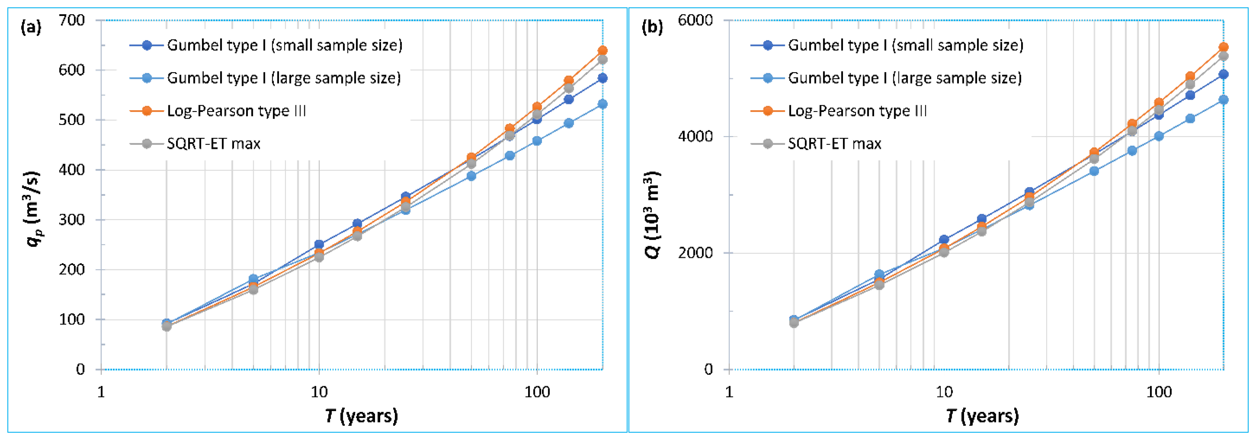
The precipitation loss function used for effective rainfall estimation is the USDA-SCS curve number method (Figure 2). To calculate the CN, the area-weighted arithmetic mean for each sub-basin has been obtained, result of the parceling each sub-basin according to the combination of the different soil type and land cover categories present. Therefore, the pertinent subdivision of each sub-basin is also necessary for this purpose. The original USDA-SCS tables have been used for the CN assignment values [28]. Applying the precipitation loss function (CN) and the rainfall-runoff model (unit hydrograph) to each sub-basin gives the corresponding values of runoff volume (Q) (i.e., net precipitation depth multiplied by sub-basin area) and the maximum instantaneous value of the outflow hydrograph (qp). Figure 4 shows the variation in Q and qp (for the whole basin) with the return period for the four distribution functions.

3. Results and Discussion

3.1. Definition and Adjustment of Probability Distribution Functions

By applying the equations explained in Section 2 (i.e., Equations (1)–(15)) to the registered annual maximum 24 h rainfall series for the period 1972–2021, the four equations for the case study have been obtained. Table 4 shows a selected sample of the most relevant parameters of each probability distribution function.
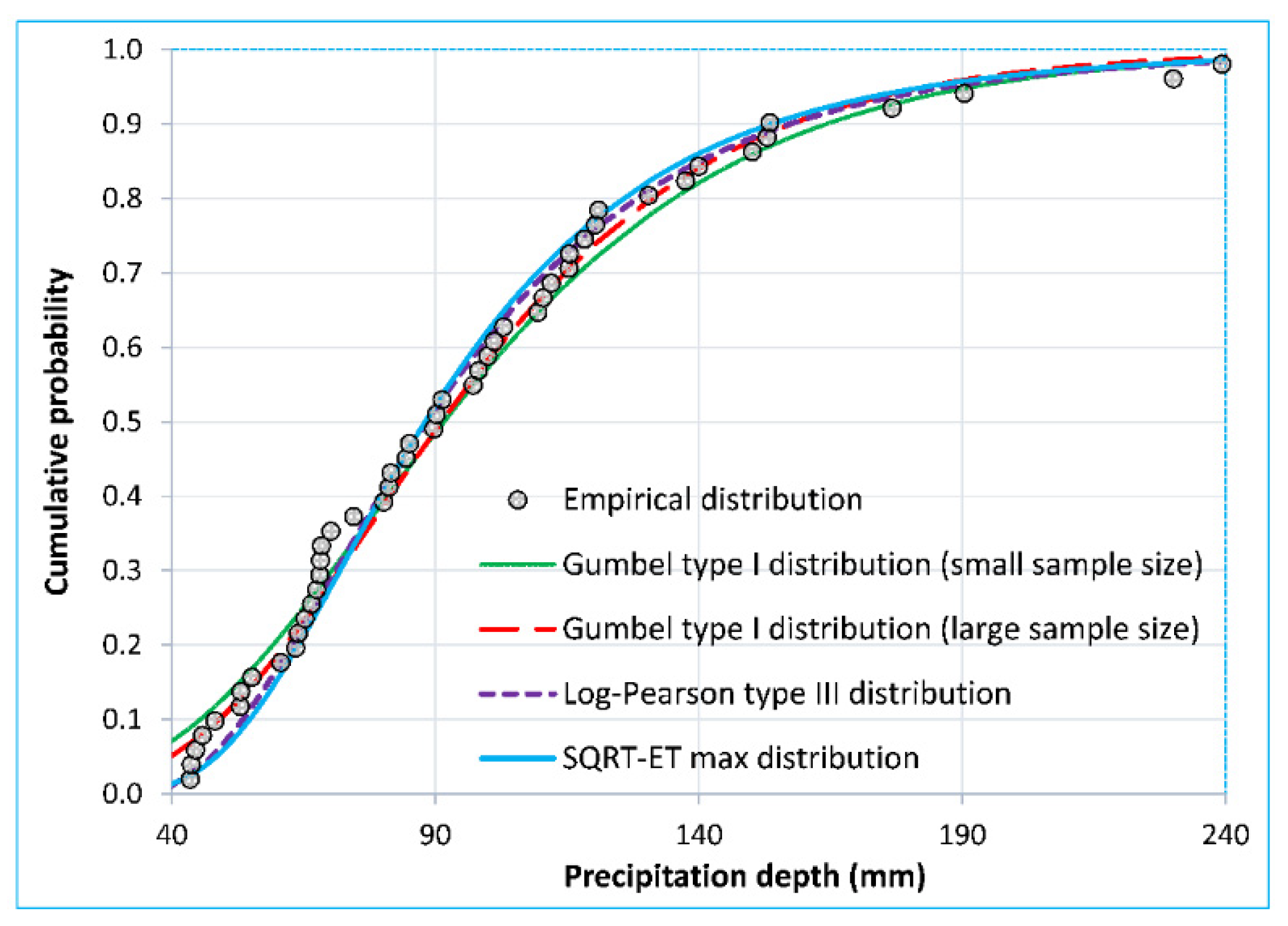
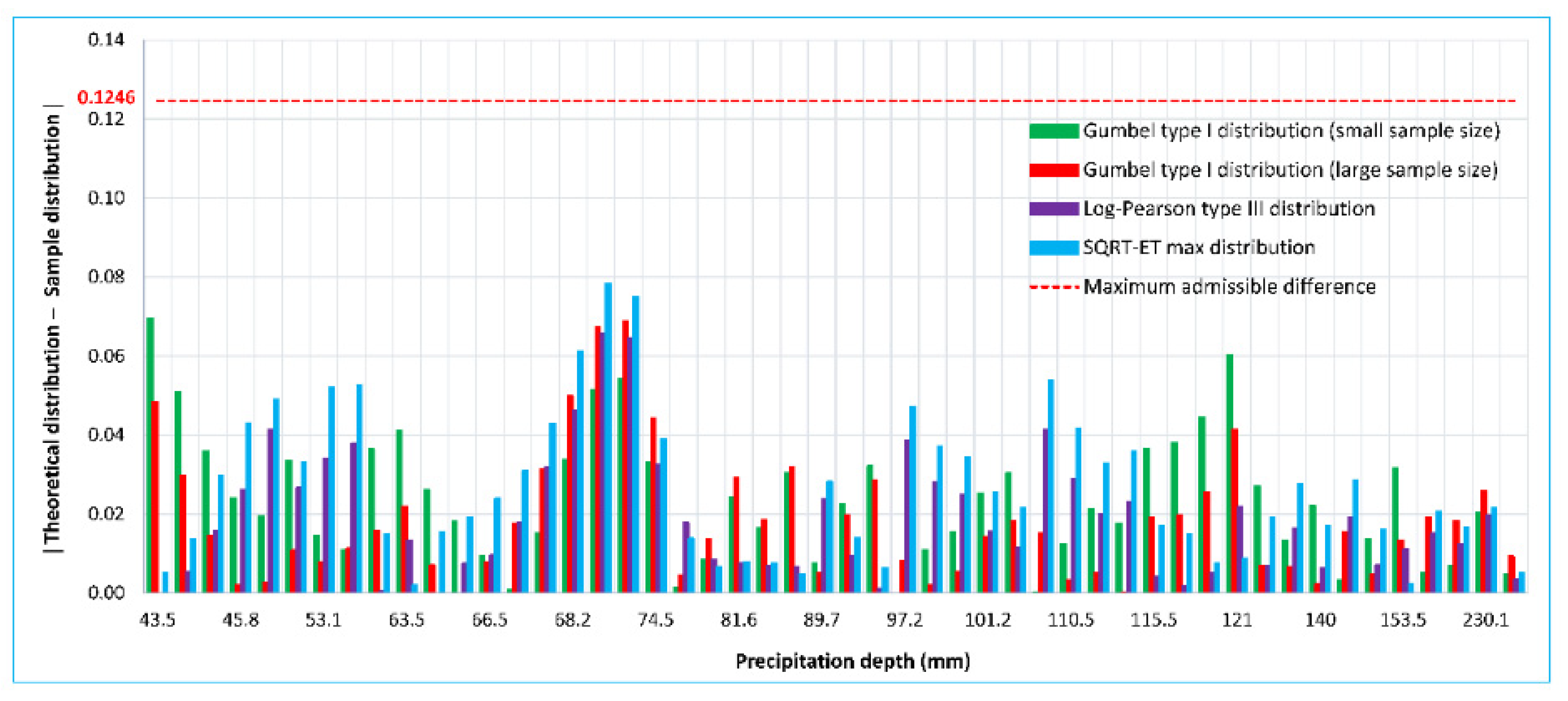
To evaluate the goodness-of-fit of the four analyzed functions, the Kolmogorov–Smirnov test (with Lilliefors criteria) is used [49]. For this purpose, the sample frequency according to the Weibull distribution should be considered [70]. Additionally, the Shapiro–Wilk test is ruled out due to the size of the sample (i.e., 50 datasets) [71]. According to [48], for n = 50 and a significance level (α) of 0.05, the maximum allowed difference is 0.1246. Due to the fact that the maximum absolute differences between the sample and theoretical distributions are located in the range 0.0690–0.0802, the goodness-of-fit is acceptable for the four functions. Among the four functions, the Gumbel type I function demonstrates the lowest difference between the sample and theoretical Weibull frequencies. Additionally, the GBS shows a difference of 0.0695 and GBL shows a value of 0.0690. Nevertheless, the LP3 and SQRT-ET present acceptable differences. The lowest adjustment appears for return periods shorter than 1.40 years for the four functions, but T values less than 2 years are not used in the probabilistic model, as explained in Section 2. Figure 5 displays a visual version of these results.
The defined distributions present small differences, as can be observed in Figure 6, where the comparison between maximum 24 h rainfall (mm) and the return period (years) for each function is shown. The intersections between the different graphics determine the changes in dominance among the functions. This dominance refers to the maximum values of rainfall for equal return periods.
Regarding the differences between functions, some conclusions can be stated. According to Figure 5, the higher differences occur for the lowest frequencies. The main differences between the distributions are evident for the first and smallest value of the series corresponding to 43.5 mm. This value has a frequency of 0.025 for the SQRT-ET and 0.089 for GBS. Furthermore, around 70 mm, a singular accumulation of values in the empirical distribution is observed. Nevertheless, these data are correct. They correspond to rainfalls between 68.1 mm and 74.5 mm. These rainfalls are numerous compared to other ranges of rainfalls. This produces a relevant increment in the sample frequency. Moreover, it must be taken into account that the study area is influenced by the Mediterranean climate. It implies relevant variations regarding the rainfall series. For this singularity, the Kolmogorov–Smirnov test (including the Lilliefors modification [48]) affects the GBS, LP3 and SQRT-ET distributions. On the contrary, the GBL presents its higher value for this test in the first dataset of the series (i.e., 43.5 mm). Nonetheless, it represents just a slight difference regarding the aforementioned singularity. Thus, it is possible to state that, regarding the control of the adjustment in this singularity interval, there are not large differences between the four distributions. Figure 7 shows the maximum differences between the analyzed empirical and theoretical distributions.
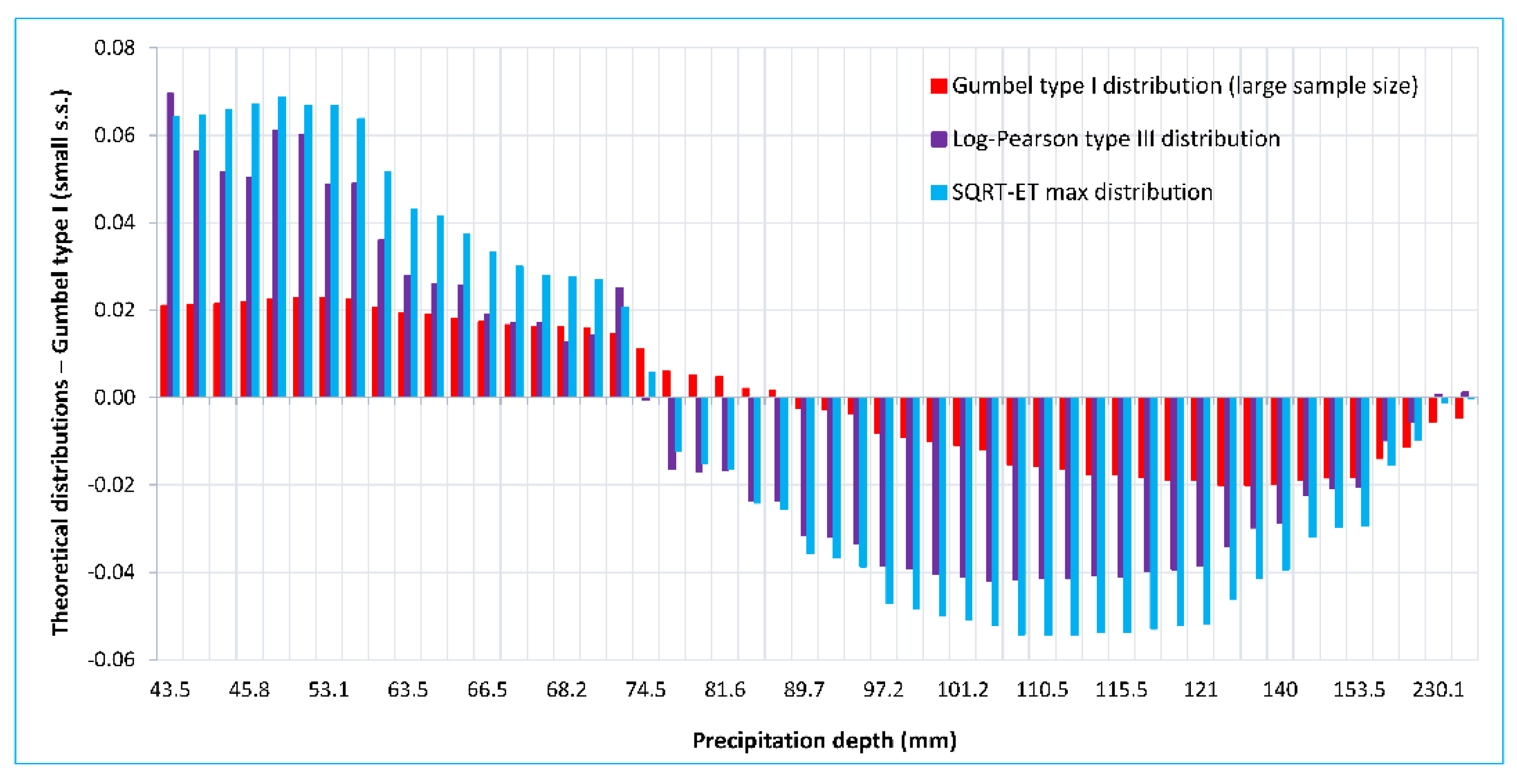
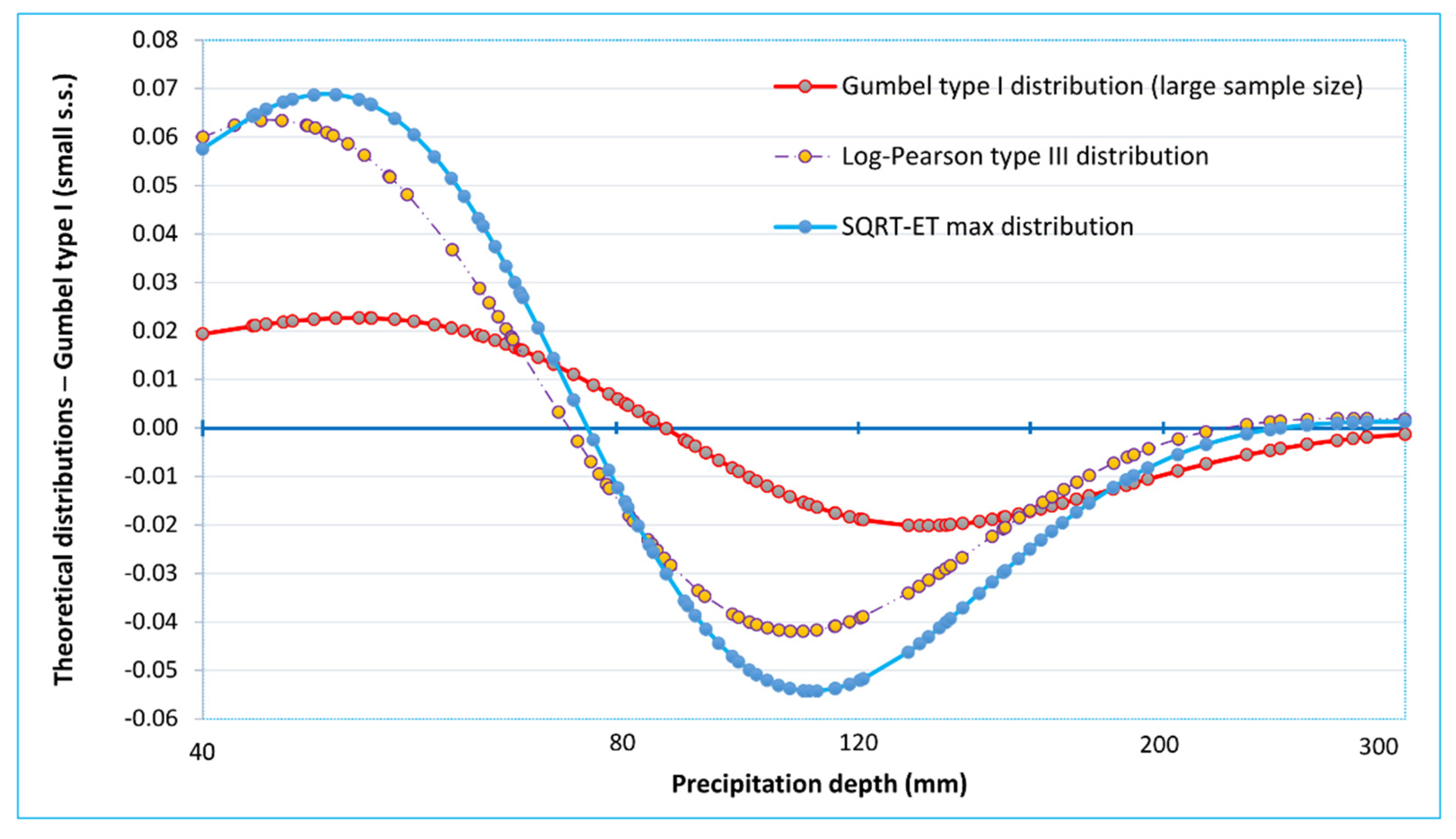
By analyzing Figure 7, it is possible to detect a decreasing trend regarding these differences between the sample and theoretical frequencies, as the precipitation depth increases. Nevertheless, these differences are too irregular and inconclusive to establish a tendency line. Consequently, Figure 8 is obtained by comparing the differences between the frequencies of the theoretical GBS distribution. This distribution is used as a reference with regard to the other three distributions and includes the precipitation depth on the horizontal axis.
A variable trend can be observed in Figure 8, demonstrating sign alternations regarding the differences, as well as an oscillatory and irregular shape. To better identify the change in tendencies, the scale of the horizontal axis of Figure 8 is modified (log scale), thereby obtaining Figure 9. The representation of precipitation depth is not limited to the sample and is extended to T = 500 years. Each point of the distribution represents the difference in its theoretical frequency with the distribution from the GBS.
The differences between the GBS (used as a reference) and the other three distributions show a progressive sign change, from positive to negative. In the case of LP3 and SQRT-ET, about 230–245 mm, the differences are positive again. In contrast, for the GBL, the differences are negative from 87 mm and they do not change.
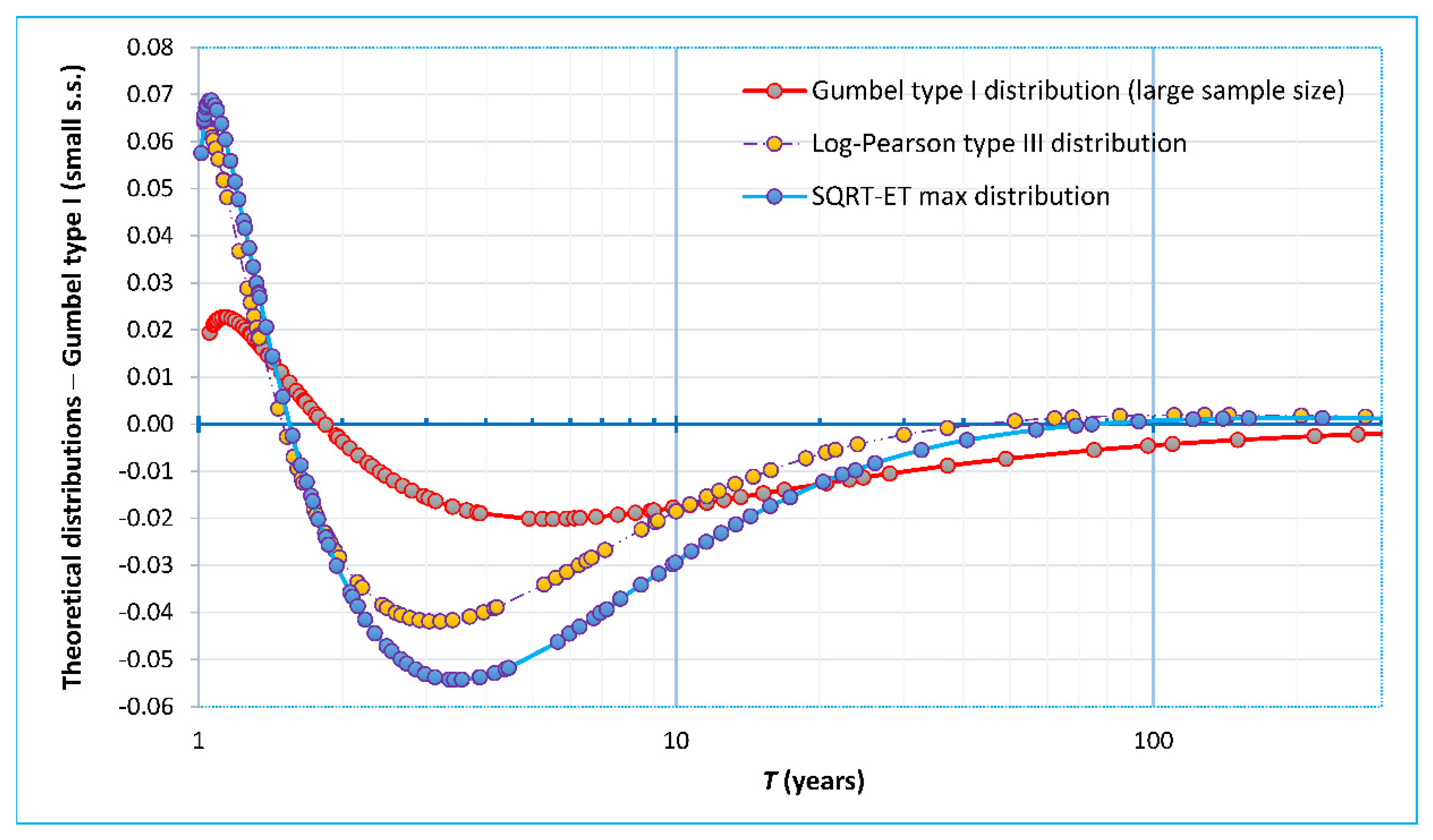
In Figure 10, each point of the distribution represents the difference in its theoretical frequency with the distribution from the GBS for a given return period (T). In Figure 10, it can be observed that for low values of T (until 51 years for LP3, and 57 years for SQRT-ET), the differences between theoretical frequencies, with regard to the GBS, are negative.
From Figure 9 and Figure 10, it can be concluded that the GBS provides larger values of annual maximum 24 h rainfall for a specific range of T. In the case of the LP3, this range could be between T = 1.5 and 51 years. In the case of the SQRT-ET, this range could be between T = 1.5 and 74 years. In the case of the GBL, since T = 2 years, the GBS provides larger values of annual maximum 24 h rainfall. Intervals shorter than T = 2 years are not relevant for the calculation with the probabilistic model, as explained in Section 2.3.

3.2. Sediment Yield for Different Return Periods

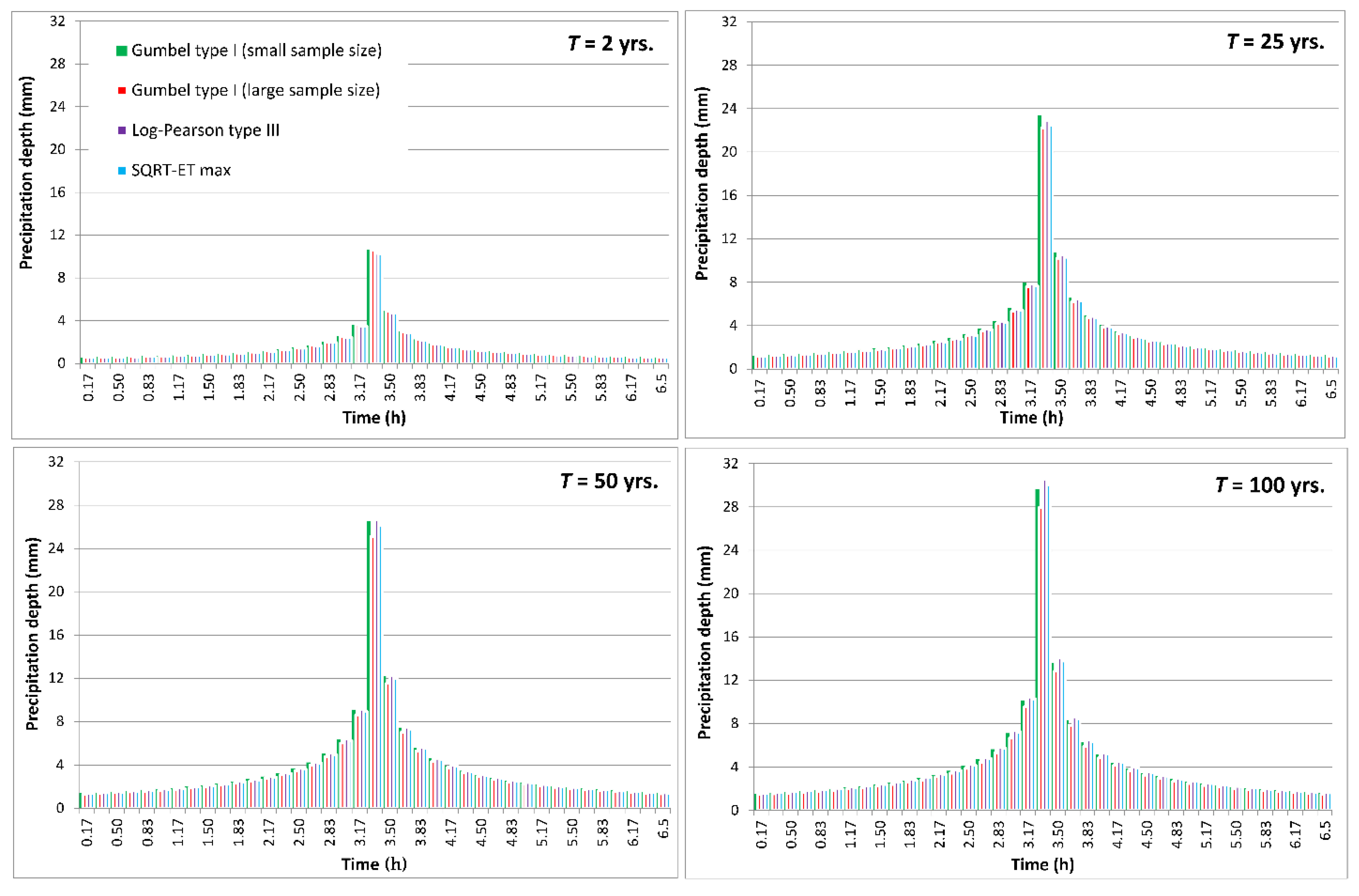
According to the developed methodology (Figure 2), to estimate the mean annual sediment yield, it is necessary to calculate the yield for each of the return periods that represent the extremes of the defined intervals. This computing process is performed separately for each probability distribution function. The four distribution functions and the series of T = 2, 5, 10, 15, 25, 50, 75, 100, 140 and 200 years must be combined in order to produce 40 design hyetographs. Figure 11 shows, as an example, the selection of four different T values (2, 25, 50 and 100).
According to Figure 11 for T < 50 years, the design hyetographs of the GBS present higher values. The hegemony of the hyetographs that correspond to the LP3 is evident when T = 50 years, approximately. This is emphasized as T increases. It implies that the values of the flow discharge obtained with the LP3 when T > 50 years will be larger than the other distributions. The sediment yield is coupled to the flow discharge, but not linearly [24]. For this reason, the emission of sediment is also higher for a design storm of T ≥ 50 years, if it is calculated according to the LP3. Nevertheless, the value of the total mean annual sediment yield of the basin calculated according to the LP3 is not the largest of the four functions.
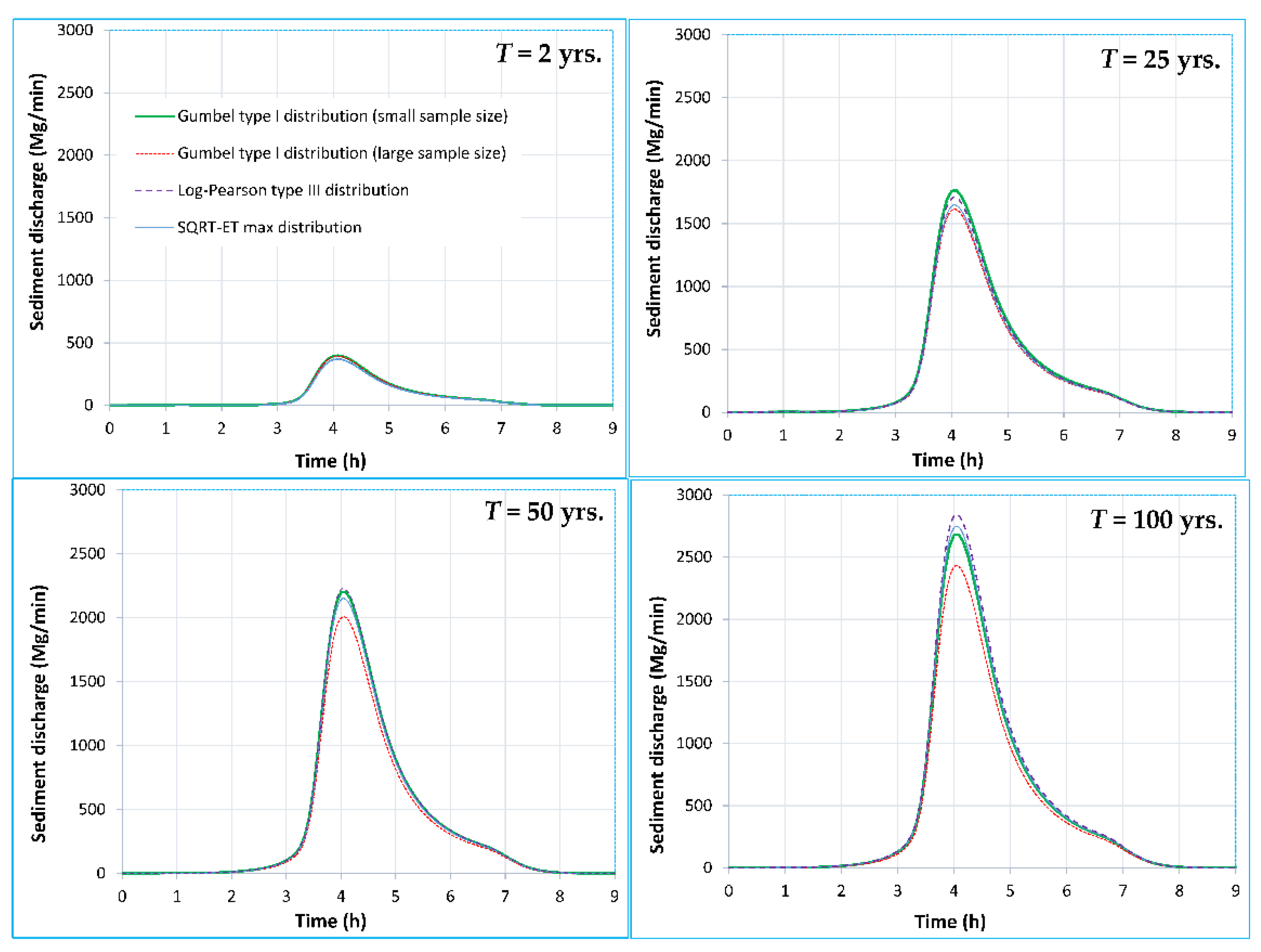
To demonstrate the first statement, the MUSLE model is implemented for the basin of Alto Palmones. Applying the HEC-HMS [27], it is possible to obtain the output sediment graphs for the basin according to each T and associated distribution function. The capability and robustness of HEC-HMS for the calculation of sediment yield has been demonstrated by Pak et al. [44]. Additionally, the influence of steep slopes does not limit its use. Other tools such as SWAT, as indicated by Rivera-Toral et al. [14], may present problems for slopes > 25% regarding the topographic factor.
To corroborate the second statement, the results of the mean annual sediment yield are presented in Section 3.3. Previously, sediment graphs for the T series used in this study were required. Figure 12 shows the sediment graphs according to the four distribution functions and a selected T series.
The application of Equation (16) requires the sediment graphs that correspond to T = 2, 5, 10, 15, 25, 50, 75, 100, 140 and 200 years. Indeed, to calculate the volume of sediments emitted, the curve of the sediment graph that corresponds to each return period Ti is integrated. The total mean annual sediment yield is doubly coupled to T [24] by the runoff generated by the different design storms, but also by the probability of occurrence associated with these design storms. This will affect the relationship between the mean annual yield and return period, meaning it will be non-linear, as can be observed in Section 3.3.
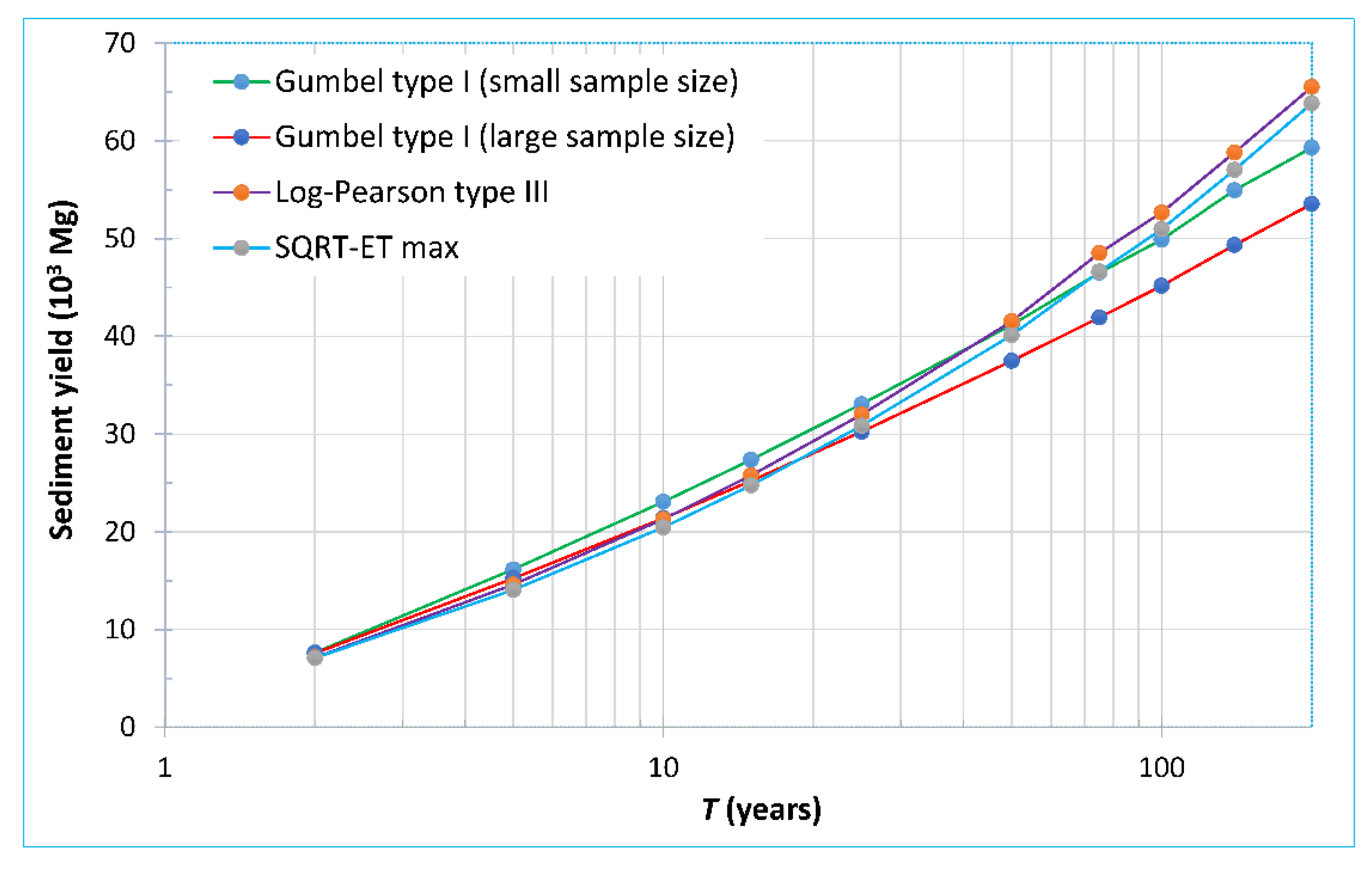
It is possible to prove that for values of T < 25 years, GBS provides the larger values of sediment emission. Since T = 50 years, the hegemony of the LP3 stands out and increases according to the return period. The emission results follow a non-linear trend, as mentioned in the previous paragraph. Figure 13 shows the sediment yield values for the four probability distribution functions as a function of the return period.
By analyzing Figure 13, it is possible to observe the clear non-linear performance in the emission-return period ratio. The higher emission values are obtained for T < 50 years with the GBS, and for T > 50 years for LP3. Furthermore, it can be observed that for T < 50 years, in the case study, GBS shows yield values on the conservative side; moreover, LP3 presents higher values of sediment yield for T > 50 years. Nevertheless, LP3 does not imply a larger total mean annual sediment yield. For further analysis, the results from Section 3.3 are needed.

3.3. Mean Annual Sediment Yield According to Each Distribution Function

As explained in Section 2.3, to calculate the sediment yield for a single rainfall event, HEC-HMS is used, which has the MUSLE model implemented (i.e., Equation (18)). The total mean annual sediment yield (Mg) is calculated with the application of Equation (16), or in a simpler way, with Equation (17). Table 5 shows the partial and total results of the application of Equations (16) and (17) for the four distribution functions studied in combination with the T series considered.
According to the previous statements and results, it is possible to determine which is the preferable probability distribution function to estimate the mean annual sediment yield of the study basin. In the case of ungauged basins (with respect to sediment emission) and for practical applications (e.g., design, operation or maintenance of infrastructures), the safe or conservative function (i.e., higher values) usually prevails. In this sense, the GBS data function provides the highest value (25,940 Mg·ha−1·y−1), and the SQRT-ET function presents the lowest (23,512 Mg·ha−1·y−1). Regarding the LP3, which is frequently used in the USA and other countries [35,59], the GBS data function provides a mean annual yield value that is 6.7% higher. With regard to the SQRT-ET function, which is frequently used in Spain [52,62], the differences reach 10%, for which the GBS obtained the highest value. The results must be analyzed cautiously, due to the fact that T values < 2 years and > 200 years have not been considered. Furthermore, the study area imposes its own restrictions (geological, edaphic, climatic and biologic ones). It is not possible to infer a law; thus, it is not possible to state a function. Nevertheless, there is mathematical certitude regarding the case study. In the context of hydrometeorological estimation of sediment yield, the LP3 and SQRT-ET functions do not provide higher values than those obtained with the GBS. Moreover, GBL presents results that are not on the safe or conservative side compared to LP3, or that are not relevant regarding SQRT-ET (Table 5). Some researchers advocate the abandonment of the Gumbel function in statistical hydrology. In this regard, Lettenmaier and Burges [57] propose to avoid the use of the GBL function (i.e., infinite sample assumption) and replace it with the GBS function (i.e., finite sample assumption). This approach is corroborated by the findings of the present research, and we, therefore, cannot justify the abandonment of the Gumbel function per se, but recommend that the sample size should be taken into account in the calculation of the distribution (i.e., as is the case for the GBS function given by Equations (2)–(4)). Indeed, according to our results, for the special case of the hydrometeorological estimation of sediment yield, the use of the GBS function would be preferable compared to the other functions analyzed, if the aim is to obtain predictions on the safe side. Even so, the differences between the predicted sediment yield values are only moderate (maximum value of 10%), which does not allow us to categorically discourage the use of any of the distribution functions analyzed.

4. Conclusions

In this study, mean annual sediment yield from a basin is estimated by applying a hydrometeorological methodology in which a probability distribution function for different intervals formed by a series of selected return periods is required. All the analyzed distribution functions present good adjustments to the sample data, even though the Gumbel type I function with a large sample size presents a slight advantage in the Kolmogorov–Smirnov test (considering the Lilliefors correction). The common simplification method for the Gumbel type I function, where the amount of data from the sample is considered to be infinite [47,50] (even by Gumbel [46]), which also implies the use of μy = 0.5772 and βy = 1.2825, does not translate into an advantage when calculating the mean annual sediment yield. Nevertheless, due to the minimal differences between the distributions, the usage of a safety coefficient of 1.07 can solve this issue.
The estimation of the mean annual sediment yield based on safe-side criteria can be approached by applying the probability distribution functions for different intervals of the return periods selected. In particular, for the case study, the used formulation and the considered intervals for T, the use of the Gumbel type I function (small sample size) resulted in the highest values. The difference in the estimated value of the total mean annual sediment yield between the four distribution functions ranged between 1% and 10%. These differences refer to some of the possible combinations of pairs of compared functions. In any case, these differences are only slight or moderate considering the general limitations in the predictive power of the model. However, based on these results, it is possible to advise against the generic abandonment of the Gumbel function per se. The highest differences occurred between the Gumbel type I (small sample size) and the SQRT-ET max functions (closely followed by Gumbel type I (large sample size)). Consequently, the log-Pearson type III and SQRT-ET max functions are not the most reliable for any of the cases from an engineering point of view (e.g., conservative side) when estimating the mean annual sediment yield using hydrometeorological methods for a generic ungauged basin.

Author Contributions

Conceptualization, C.A.R.G.; methodology, C.A.R.G. and Á.M.R.-P.; software, C.A.R.G., J.J.C.-M. and J.A.H.-T.; formal analysis, C.A.R.G., Á.M.R.-P. and R.L.; investigation, C.A.R.G. and R.L.; resources, C.A.R.G. and Á.M.R.-P.; data curation, Á.M.R.-P., J.J.C.-M. and J.A.H.-T.; writing—original draft preparation, C.A.R.G. and R.L.; writing—review and editing, R.L. and C.A.R.G.; visualization, R.L., Á.M.R.-P., J.J.C.-M. and J.A.H.-T.; supervision, R.L.; project administration, C.A.R.G. All authors have read and agreed to the published version of the manuscript.

Funding

This research received no external funding.

Data Availability Statement

Data are contained within the article. The tool files used for this study are available upon request from the corresponding author.

Acknowledgments

The authors would like to thank Deryck J. Barker Fraser for the translation of the manuscript. The third author acknowledges the support of the Catalan Government through the Fluvial Dynamics Research Group (RIUS 2017 SGR 459).

Conflicts of Interest

The authors declare no conflict of interest.

References

  1. Nearing, M.A.; Xie, Y.; Liu, B.; Ye, Y. Natural and anthropogenic rates of soil erosion. Int. Soil Water Conserv. Res. 2017, 5, 77–84. [Google Scholar] [CrossRef]
  2. Quine, T.A.; Walling, D.E.; Zhang, X. Tillage erosion, water erosion and soil quality on cultivated terraces near Xifeng in the Loess Plateau, China. Land Degrad. Dev. 1999, 10, 251–274. [Google Scholar] [CrossRef]
  3. Mishra, P.K.; Rai, A.; Abdelrahman, K.; Rai, S.C.; Tiwari, A. Land Degradation, Overland Flow, Soil Erosion, and Nutrient Loss in the Eastern Himalayas, India. Land 2022, 11, 179. [Google Scholar] [CrossRef]
  4. Butt, M.J.; Waqas, A.; Mahmood, R. The combined effect of vegetation and soil erosion in the water resource management. Water Resour. Manag. 2010, 24, 3701–3714. [Google Scholar] [CrossRef]
  5. Gemitzi, A.; Petalas, C.; Tsihrintzis, V.A.; Pisinaras, V. Assessment of groundwater vulnerability to pollution: A combination of GIS, fuzzy logic and decision making techniques. Environ. Geol. 2006, 49, 653–673. [Google Scholar] [CrossRef]
  6. Halbac-Cotoara-Zamfir, R.; Smiraglia, D.; Quaranta, G.; Salvia, R.; Salvati, L.; Giménez-Morera, A. Land degradation and mitigation policies in the Mediterranean region: A brief commentary. Sustainability 2020, 12, 8313. [Google Scholar] [CrossRef]
  7. European Parlament. Procedure File: 2021/2548(RSP)|Legislative Observatory. 2021. Available online: https://oeil.secure.europarl.europa.eu/oeil/popups/ficheprocedure.do?reference=2021/2548(RSP)&l=en (accessed on 5 November 2022).
  8. Djoukbala, O.; Hasbaia, M.; Benselama, O.; Mazour, M. Comparison of the erosion prediction models from USLE, MUSLE and RUSLE in a Mediterranean watershed, case of Wadi Gazouana (NW of Algeria). Model. Earth Syst. Environ. 2019, 5, 725–743. [Google Scholar] [CrossRef]
  9. Busari, M.A.; Kukal, S.S.; Kaur, A.; Bhatt, R.; Dulazi, A.A. Conservation tillage impacts on soil, crop and the environment. Int. Soil Water Conserv. Res. 2015, 3, 119–129. [Google Scholar] [CrossRef] [Green Version]
  10. Wischmeier, W.H.; Smith, D.D. A Universal Soil-Loss Equation to guide conservation farm planning. Trans. 7th Int. Congr. Soil Sci. 1960, 1, 418–425. [Google Scholar]
  11. RUSLE2. Conservation Planning, Inventory Erosion Rates and Estimate Sediment Delivery. NRCS, USDA, USA. Available online: https://fargo.nserl.purdue.edu/rusle2_dataweb/About_RUSLE2_Technology.htm (accessed on 11 November 2022).
  12. Akoko, G.; Le, T.H.; Gomi, T.; Kato, T. A review of SWAT model application in Africa. Water 2021, 13, 1313. [Google Scholar] [CrossRef]
  13. Gassman, P.W.; Sadeghi, A.M.; Srinivasan, R. Applications of the SWAT model special section: Overview and insights. J. Environ. Qual. 2014, 43, 1–8. [Google Scholar] [CrossRef] [PubMed]
  14. Rivera-Toral, F.; Pérez-Nieto, S.; Ibáñez-Castillo, L.A.; Hernández-Saucedo, F.R. Aplicabilidad del Modelo SWAT para la estimación de la erosión hídrica en las cuencas de México. Agrociencia 2012, 46, 101–105. Available online: http://www.scielo.org.mx/scielo.php?script=sci_arttext&pid=S1405-31952012000200001&lng=es&nrm=iso (accessed on 4 September 2022).
  15. Sadeghi, S.H.R.; Gholami, L.; Khaledi Darvishan, A.; Saeidi, P. A review of the application of the MUSLE model worldwide. Hydrol. Sci. J. 2014, 59, 365–375. [Google Scholar] [CrossRef] [Green Version]
  16. Williams, J.R.; Berndt, H.D. Sediment yield prediction based on watershed hydrology. Trans. ASAE 1977, 20, 1100–1104. [Google Scholar] [CrossRef]
  17. Arekhi, S.; Shabani, A.; Rostamizad, G. Application of the Modified Universal Soil Loss equation (MUSLE) in prediction of sediment yield (Case study: Kengir Watershed, Iran). Arab. J. Geosci. 2012, 5, 1259–1267. [Google Scholar] [CrossRef]
  18. Berteni, F.; Dada, A.; Grossi, G. Application of the MUSLE model and potential effects of climate change in a small alpine catchment in northern Italy. Water 2021, 13, 2679. [Google Scholar] [CrossRef]
  19. Pongsai, S.; Schmidt Vogt, D.; Shrestha, R.P.; Clemente, R.S.; Eiumnoh, A. Calibration and validation of the Modified Universal Soil Loss Equation for estimating sediment yield on sloping plots: A case study in Khun Satan catchment of northern Thailand. Can. J. Soil Sci. 2010, 90, 585–596. [Google Scholar] [CrossRef] [Green Version]
  20. Odongo, V.O.; Onyando, J.O.; Mutua, B.M.; Becht, R. Sensitivity analysis and calibration of the Modified Universal Soil Loss Equation (MUSLE) for the upper Malewa catchment, Kenya. Int. J. Sediment Res. 2013, 28, 368–383. [Google Scholar] [CrossRef]
  21. Rodríguez, A.; García, J.L.; Robredo, J.C.; López, D. Specific sediment yield model for reservoirs with medium-sized basins in Spain: An empirical and statistical approach. Sci. Total Environ. 2019, 681, 82–101. [Google Scholar] [CrossRef]
  22. Hrissanthou, V. Estimate of sediment yield in a basin without sediment data. Catena 2005, 64, 333–347. [Google Scholar] [CrossRef]
  23. García, C.; Robredo, J.C. Metodología para la evaluación de la emisión interanual de sedimentos por una cuenca vertiente. Rev. Montes 1996, 45, 22–24. [Google Scholar]
  24. Rodríguez, C.A.; Rodríguez-Pérez, Á.M.; Mancera, J.; Torres, J.; Carmona, N.; Bahamonde García, M. Applied methodology based on HEC-HMS for reservoir filling estimation due to soil erosion. J. Hydrol. Hydromech. 2022, 70, 341–356. [Google Scholar] [CrossRef]
  25. Williams, J.R. Sediment-yield prediction with universal equation using runoff energy factor. In Present and Prospective Technology for Predicting Sediment Yield and Sources; US Department of Agriculture, Agriculture Research Service: Washington, DC, USA, 1975; pp. 244–252. [Google Scholar]
  26. Lu, J.; Zheng, F.; Li, G.; Bian, F.; An, J. The effects of raindrop impact and runoff detachment on hillslope soil erosion and soil aggregate loss in the Mollisol region of Northeast China. Soil Tillage Res. 2016, 161, 79–85. [Google Scholar] [CrossRef]
  27. HEC–HMS (Hydrologic Engineering Center–Hydrologic Modeling System), 4.10 [Computer Software] ed; Army Corps of Engineers: Davis, CA, USA, 2022; Available online: http://www.hec.usace.army.mil/ (accessed on 10 October 2022).
  28. HEC-HMS (Hydrologic Engineering Center–Hydrologic Modeling System). Technical Reference Manual. CN Tables. Available online: https://www.hec.usace.army.mil/confluence/hmsdocs/hmstrm/cn-tables (accessed on 14 November 2022).
  29. Shi, W.; Chen, T.; Yang, J.; Lou, Q.; Liu, M. An improved MUSLE model incorporating the estimated runoff and peak discharge predicted sediment yield at the watershed scale on the Chinese Loess Plateau. J. Hydrol. 2022, 614, 128598. [Google Scholar] [CrossRef]
  30. Chimene, C.A.; Campos, J.N.B. The design flood under two approaches: Synthetic storm hyetograph and observed storm hyetograph. J. Appl. Water Eng. Res. 2020, 8, 171–182. [Google Scholar] [CrossRef]
  31. Watt, E.; Marsalek, J. Critical review of the evolution of the design storm event concept. Can. J. Civ. Eng. 2013, 40, 105–113. [Google Scholar] [CrossRef]
  32. Yen, B.C.; Chow, V.T. Design hyetographs for small drainage structures. J. Hydraul. Div. 1980, 106, 1055–1076. [Google Scholar] [CrossRef]
  33. Chow, V.T.; Maidment, D.R.; Mays, L.W. Applied Hydrology; McGraw-Hill: New York, NY, USA, 1988. [Google Scholar]
  34. Ilić, A.; Plavšić, J.; Radivojević, D. Rainfall-runoff simulation for design flood estimation in small river catchments. Facta Universitatis. Ser. Archit. Civ. Eng. 2018, 16, 029–043. [Google Scholar] [CrossRef] [Green Version]
  35. Maity, R. Probability Distributions and Their Applications. In Civil and Environmental Engineering; Springer: Singapore, 2018; pp. 93–143. [Google Scholar] [CrossRef]
  36. Haan, C.T. Statistical Methods in Hydrology, 2nd ed.; Iowa State University Press: Ames, IA, USA, 2002. [Google Scholar]
  37. Stedinger, J.R.; Vogel, R.M.; Foufoula-Georgiou, E. Chapter 18. Frequency analysis of extreme events. In Handbook of Hydrology; Editor in Chief David R. Maidment; McGraw-Hill: New York, NY, USA, 1993. [Google Scholar]
  38. Ministerio Para la Transición Ecológica y el Reto Demográfico. Gobierno de España. Reserva Natural Fluvial Alto Palmones. Available online: https://www.miteco.gob.es/es/agua/temas/delimitacion-y-restauracion-del-dominio-publico-hidraulico/Catalogo-Nacional-de-Reservas-Hidrologicas/informacion/andalucia/alto-palmones/default.aspx (accessed on 8 November 2022).
  39. Ministerio Para la Transición Ecológica y el Reto Demográfico. Gobierno de España. Agencia Estatal de Meteorología. Available online: https://www.aemet.es/en/serviciosclimaticos (accessed on 3 September 2021).
  40. Consejería de Agricultura, Ganadería, Pesca y Desarrollo Sostenible. Junta de Andalucía. Catálogo de la Red de Información Ambiental de Andalucía (REDIAM). Available online: https://www.juntadeandalucia.es/medioambiente/portal/acceso-rediam (accessed on 29 November 2022).
  41. Ministerio de Ciencia de Innovación. CSIC. Instituto Geológico y Minero de España. Gobierno de España. Información Geocientífica del IGME. Available online: http://info.igme.es/catalogo/default.aspx?lang=spa (accessed on 11 November 2022).
  42. QGIS. A Free and Open Source Geographic Information System. Available online: https://www.qgis.org/en/site/ (accessed on 8 November 2022).
  43. Steinmetz, A.A.; Beskow, S.; Terra, F.D.S.; Nunes, M.C.M.; Vargas, M.M.; Horn, J.F.C. Spatial discretization influence on flood modeling using unit hydrograph theory. RBRH 2019, 24, 1–12. [Google Scholar] [CrossRef] [Green Version]
  44. Pak, J.H.; Fleming, M.; Scharffenberg, W.; Gibson, S.; Brauer, T. Modeling surface soil erosion and sediment transport processes in the upper North Bosque River Watershed, Texas. J. Hydrol. Eng. 2015, 20, 04015034. [Google Scholar] [CrossRef]
  45. Pak, J.H.; Ramos, K.; Fleming, M.; Scharffenberg, W.; Gibson, S. Sensitivity Analysis for Sediment Transport in the Hydrologic Modeling System (HEC-HMS). Proc., Joint Federal Interagency Conf. 2015. Available online: https://acwi.gov/sos/pubs/3rdJFIC/Contents/2A-Pak.pdf (accessed on 8 November 2022).
  46. Gumbel, E.J. The return period of flood flows. Ann. Math. Stat. 1941, 12, 163–190. Available online: https://www.jstor.org/stable/2235766 (accessed on 9 November 2022). [CrossRef]
  47. Wanielista, M.; Robert, K.; Ron, E. Hydrology: Water Quantity and Quality Control; John Wiley and Sons: Hoboken, NJ, USA, 1997. [Google Scholar]
  48. Molin, P.; Abdi, H. New Table and Numerical Approximations for Kolmogorov-Smirnov/Lilliefors/van Soest Normality Test; University of Bourgogne: Dijon, France, 1998; Available online: https://personal.utdallas.edu/~herve/MolinAbdi1998-LillieforsTechReport.pdf (accessed on 24 October 2022).
  49. Lilliefors, H.W. On the Kolmogorov-Smirnov test for normality with mean and variance unknown. JASA 1967, 62, 399–402. [Google Scholar] [CrossRef]
  50. Huang, Y.P.; Lee, C.H.; Ting, C.S. Improved estimation of hydrologic data using the chi-square goodness-of-fit test. J. Chin. Instig. Eng. 2008, 31, 515–521. [Google Scholar] [CrossRef]
  51. Coronado-Hernández, Ó.E.; Merlano-Sabalza, E.; Díaz-Vergara, Z.; Coronado-Hernández, J.R. Selection of hydrological probability distributions for extreme rainfall events in the regions of Colombia. Water 2020, 12, 1397. [Google Scholar] [CrossRef]
  52. Zorraquino, C. La función SQRT-ET max. Revista de Obras Públicas 2004, 3447, 33–37. [Google Scholar]
  53. Ferrer, F.J. El Modelo de Función de Distribución SQRT et MAX en el Análisis Regional de Máximos Hidrológicos. Aplicación a Lluvias Diarias. Ph.D. Thesis, Universidad Politécnica de Madrid, Madrid, Spain, 1996. [Google Scholar]
  54. Carter, D.J.T.; Challenor, P.G. Methods of fitting the Fisher-Tippett type 1 extreme value distribution. Ocean Eng. 1983, 10, 191–199. [Google Scholar] [CrossRef]
  55. Gumbel, E.J. Les valeurs extrêmes des distributions statistiques. Annales de l’institut Henri Poincaré 1935, 5, 115–158. Available online: http://www.numdam.org/item/AIHP_1935__5_2_115_0.pdf (accessed on 9 November 2022).
  56. Lehmer, D.H. Euler constants for arithmetical progressions. Acta Arith. 1975, 27, 25–142. [Google Scholar] [CrossRef] [Green Version]
  57. Lettenmaier, D.P.; Burges, S.J. Gumbel’s extreme value I distribution: A new look. J. Hydraul. Eng. 1982, 108, 502–514. [Google Scholar] [CrossRef]
  58. Pearson, K. Contributions to the mathematical theory of evolution. Philos. Trans. R. Soc. 1894, 185, 71–110. [Google Scholar] [CrossRef] [Green Version]
  59. Huynh, N.P.; Thambirajah, J.A. Applications of the log Pearson type-3 distribution in hydrology. J. Hydrol. 1984, 73, 359–372. [Google Scholar] [CrossRef]
  60. Bobee, B.B.; Robitaille, R. The use of the Pearson type 3 and log Pearson type 3 distributions revisited. Water Resour. Res. 1977, 13, 427–443. [Google Scholar] [CrossRef]
  61. Etoh, T.; Murota, A.; Nakanishi, M. SQRT-exponential type distribution of maximum. In Hydrologic Frequency Modeling; Springer: Dordrecht, The Netherlands, 1987; pp. 253–264. [Google Scholar]
  62. Ferrer, F.J. Recomendaciones Para el Cálculo Hidrometeorológico de Avenidas. Ed. CEDEX, Spain. 2000. Available online: https://hispagua.cedex.es/node/92786 (accessed on 24 October 2022).
  63. Ministerio de Fomento. Dirección General de Carreteras. Gobierno de España. Máximas Lluvias Diarias en la España Peninsular. Ed. Secretaría de Estado de Infraestructuras y Transportes, Spain. 1999. Available online: https://www.mitma.gob.es/recursos_mfom/0610300.pdf (accessed on 24 October 2022).
  64. Kaffas, K.; Hrissanthou, V. Annual sediment yield prediction by means of three soil erosion models at the basin scale. In Proceedings of the 10th World Congress of EWRA “Panta Rhei”, Athens, Greece, 5–9 July 2017; pp. 5–9. Available online: https://www.ewra.net/ew/pdf/EW_2017_58_46.pdf (accessed on 10 November 2022).
  65. Gómez-Zotano, J.; Alcántara-Manzanares, J.; Olmedo-Cobo, J.A.; Martínez-Ibarra, E. La sistematización del clima mediterráneo: Identificación, clasificación y caracterización climática de Andalucía (España). Rev. Geogr. Norte Gd. 2015, 61, 161–180. [Google Scholar] [CrossRef] [Green Version]
  66. Trinh, T.; Kavvas, M.L.; Ishida, K.; Ercan, A.; Chen, Z.Q.; Anderson, M.L.; Nguyen, T. Integrating global land-cover and soil datasets to update saturated hydraulic conductivity parameterization in hydrologic modeling. Sci. Total Environ. 2018, 631, 279–288. [Google Scholar] [CrossRef] [PubMed]
  67. Allue Andrade, J.L. Atlas Fitoclimático de España. Taxonomías; Ministerio de Agricultura Pesca y Alimentación: Madrid, Spain, 1990. [Google Scholar]
  68. Dysarz, T.; Wicher-Dysarz, J. Application of Hydrodynamic Simulation and Frequency Analysis for Assessment of Sediment Deposition and Vegetation Impacts on Floodplain Inundation. Pol. J. Environ. Stud. 2011, 20, 1441–1451. Available online: http://www.pjoes.com/Application-of-Hydrodynamic-Simulation-r-nand-Frequency-Analysis-for-Assessment-r,88695,0,2.html (accessed on 11 November 2022).
  69. Témez, J.R. Facetas del cálculo hidrometeorológico y estadístico de máximos caudales. Rev. Obras Públicas 2003, 3430, 47–51. [Google Scholar]
  70. Lai, C.-D.; Murthy, D.N.; Xie, M. Weibull distributions and their applications. In Springer Handbooks; Springer: Berlin/Heidelberg, Germany, 2006; pp. 63–78. [Google Scholar] [CrossRef]
  71. Razali, N.M.; Wah, Y.B. Power comparisons of Shapiro-Wilk, Kolmogorov-Smirnov, Lilliefors and Anderson-Darling tests. JOSMA 2011, 2, 21–33. [Google Scholar]
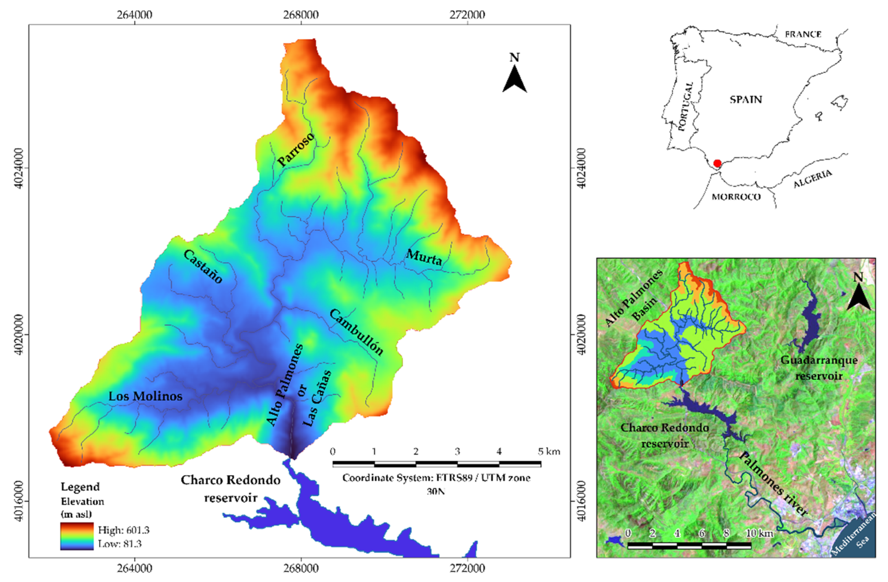
Figure 1. Location of the Alto Palmones basin.
Land 12 00035 g001
Figure 2. Flow chart of the applied methodology. Only the main operations have been represented.
Land 12 00035 g002
Figure 3. Thematic maps: (a) slope map, (b) land-cover map, (c) geological and soil map; (d) MUSLE factors.
Land 12 00035 g003
Figure 4. (a) Peak flow discharge (qp), and (b) runoff volume (Q) during return period for the probability distribution functions and for the whole basin.
Land 12 00035 g004
Figure 5. Cumulative probability against precipitation depth for the probability distribution functions.
Land 12 00035 g005
Figure 6. Precipitation depth against return period for the probability distribution functions.
Land 12 00035 g006
Figure 7. Differences between theoretical and sample distributions (absolute value) against precipitation depth.
Land 12 00035 g007
Figure 8. Differences between theoretical distributions with respect to Gumbel type I with a small sample size (small s.s.), as a reference, against precipitation depth.
Land 12 00035 g008
Figure 9. Differences between theoretical distributions with respect to Gumbel type I with a small sample size (small s.s.), as a reference, against precipitation depth. Log scale is used for horizontal axis.
Land 12 00035 g009
Figure 10. Differences between theoretical distributions with respect to Gumbel type I with a small sample size (small s.s.), as a reference, against return period.
Land 12 00035 g010
Figure 11. Design hyetographs for T = 2, 25, 50 and 100 years. The blocks that correspond to GBS are highlighted in green.
Land 12 00035 g011
Figure 12. Total outlet sediment graphs for the study basin. T = 2, 25, 50, and 100 years.
Land 12 00035 g012
Figure 13. Mean annual sediment yield for the study basin against return period.
Land 12 00035 g013
Table 1. Statistical variables of the annual maximum 24 h rainfall dataset.
Sample Size
n
Mean
(mm)
Standard Deviation (mm)CovarianceSkewness Coefficient
5098.6245.150.460.24
Table 2. Soil units (texture).
Sandy AlgibeCampo de Gibraltar Clays
Diameter (mm)Percentage Lower Than
0.000500
0.0009615
0.0021040
0.0051545
0.012050
0.0634256
0.17063
0.259075
0.59585
1100100
Table 3. Soil units (K definition).
PropertiesType of Soil
Sandy AlgibeClays of the Campo de Gibraltar
Soil textureSandy loamClayey
Soil structureSimple grain, weak and thinCrumbly and lumpy on the surface. Arranged in blocks below the surface.
Percent of organic matter1.721.93
Soil permeabilityModerateVery slow
K factor0.300.41
Table 4. Characteristic parameters of the probability distribution functions.
Gumbel Type I with a Small Sample SizeGumbel Type I with a Large Sample SizeLog-Pearson Type IIISQRT-ET Max
α (n)β (n)α ()β ()β (LP3)γ (LP3)X0 (LP3)α (SQRT)k (SQRT)
0.0259777.49910.028478.30370.052167.50270.98180.499369.3027
Table 5. Mean annual sediment yield estimation and comparative analysis.
Interval
(Years)
Probability of
Occurrence a
Average
Yield b (Mg)
Sediment Yield
Per Interval c (Mg·y−1)
GBSGBLLP3SQRT-ETGBSGBLLP3SQRT-ET
2–50.30035,70734,20832,58431,71110,71210,26297759513
5–100.10058,83554,91153,84451,7555884549153845175
10–150.03375,65869,86970,60867,8062522232923542260
15–250.02790,63783,15886,63983,4132417221823102224
25–500.020111,345101,598110,285106,4592227203222062129
50–750.007131,540119,114135,093130,102877794901867
75–1000.003144,622130,639151,789146,387482435506488
100–1400.003157,266141,779167,217161,991449405478463
140–2000.002171,394154,354186,507181,300367331400388
Total sum of mean annual sediment yield (Mg) 25,93724,29724,31323,509
a Calculated as ( 1 T i 1 T i + 1 ) ; b Calculated as 1 2 ( Y T i + Y T i + 1 ) ; c Calculated as ( 1 T i 1 T i + 1 ) 1 2 ( Y T i + Y T i + 1 ) .
Disclaimer/Publisher’s Note: The statements, opinions and data contained in all publications are solely those of the individual author(s) and contributor(s) and not of MDPI and/or the editor(s). MDPI and/or the editor(s) disclaim responsibility for any injury to people or property resulting from any ideas, methods, instructions or products referred to in the content.