Spatial Pattern of Soil Erosion in Relation to Land Use Change in a Rolling Hilly Region of Northeast China

Abstract

The black soil region in Northeast China is one of the major grain-producing areas of China. Soil erosion in the black soil region caused by natural factors and anthropic activities has attracted much attention, especially in a rolling hilly region. Compared with natural factors, the land use factor of cropland encompasses the most easily optimized measures. Jiutai County of Changchun City, located in the hilly areas of Northeast China, was taken as an example to calculate the soil erosion modulus using the Revised Universal Soil Loss Equation model. The overall soil erosion status of cultivated land in the study area was mainly slight and light, the proportion of cultivated land affected by extremely intensive and severe erosion was relatively small, and the average soil erosion modulus was 7.09 t·hm⁻²·a⁻¹ in 2019. In view of spatial distribution characteristics of soil erosion revealed by the spatial aggregation and hot spot analysis, the most serious soil erosion intensity was concentrated in the southeast and northeast sloping farmland over 8°. With the increase in elevation and topographic slope, the proportion of slight and light soil erosion gradually decreased, which was closely related to the increase in soil erodibility caused by the space–time migration of soil organic carbon caused by the interaction of hydraulic and tillage erosion in complex topographic areas. The Geographically Weighted Regression model was introduced to explore the driving factors and superposition mechanism of farmland soil erosion in the hilly region of Northeast China. Based on the relationship between soil erosion and landscape fragmentation, landscape fragmentation was an important driving force promoting soil erosion, sediment yield, and sediment transport. This paper is committed to providing a basis for accurately deploying regional soil and water conservation measures and formulating macro land management policies.

1. Introduction

Soil erosion has become a major factor driving soil degradation processes [1], affecting soil and nutrient loss at original sites and accumulation at deposition sites [2,3]. Soil erosion results in nutrient loss through the denudation of surface soil and soil organic matter, which not only leads to land degradation and fertility loss but also influences the corresponding biogeochemical cycles (the siltation and eutrophication of water environment, enhancement of flooding, and decrease or increase in CO₂ emissions) [4]. For example, Hancock and Wells using a flume experiment suggested that soil organic carbon (SOC) is enriched in eroded sediment [5]. Soil erosion alters the biological process of SOC mineralization resulting in the loss of C from the soil to the atmosphere [6]. The disturbance of soil erosion in the terrestrial carbon cycle also restricts the buffering effect of the soil ecosystem on climate change and further affects the global ecosystem security [7,8]. China is one of the countries with the worst soil erosion phenomenon in the world [9], according to the Ministry of Water Resources, which issued the second national soil erosion remote sensing survey results showing that the national soil erosion area reached 3.56 million km². Moreover, the problem of soil erosion in the black soil area of Northeast China has attracted extensive attention [10,11].

Soil erosion is derived from the joint effect of natural and human influencing factors [12]. Land use is the most important predictor of soil erosion susceptibility, which can slow down or speed up soil erosion, depending on the specific situation [13]. Irrational land use is one of the substantial factors that accelerate regional soil erosion [14]. Understanding the impact of land use changes on soil erosion is crucial for exploring the mechanism of regional erosion and identifying the driving forces of anthropogenic controllable erosion [15,16,17]. Most studies regarding the response of soil erosion to land use change focus on the estimation of soil erosion of different land use types [18,19], but an exploration of the response of land use intensity and landscape fragmentation to soil erosion is lacking. Therefore, building on the spatial characterization of soil erosion patterns and the identification of erosion hotspots, the impacts of land use intensity and farmland landscape fragmentation on the spatial differentiation characteristics of arable land soil erosion were identified, and scientific land management methods were adopted to control regional soil erosion and improve soil quality, which is conducive to the sustainable use of land resources and achieving regional sustainable development.

The inherently fertile black soils (Mollisols) account for nearly 6.9% of the Earth’s land area. Tremendous black soils all over the world are suffering soil erosion and soil degradation due to unreasonable management and prolonged agricultural production [20,21]. However, black soil is also an abundant organic carbon (OC) pool; thus, any loss of black SOC due to global climate change is likely to produce considerable feedback [22]. The black soil region of Northeast China is crucial for grain production in China but has been threatened by intensive and extensive soil erosion due to long-term intense cultivation activity after the transformation from forest to cropland. Therefore, this paper selected the Jiutai District of Changchun City, which is located in the rolling hilly region of Northeast China. In the past few decades, although it is an important commodity grain production base in China, it has experienced severe degradation in physical [23], chemical [24], and biological properties [25], which provides a platform for examining the separated effects and influence mechanism of land use change on soil erosion, and is vital for the subsequent sustainable, optimal management of black soils in Northeast China.

In this paper, Jiutai County of Changchun City, located in the black soil region of Northeast China, was taken as an example area to carry out the soil erosion modulus using the Revised Universal Soil Loss Equation (RUSLE) and then to recognize the erosion hot spots. The Geographical Weighted Regression (GWR) model was introduced to discuss the key driving factors and superposition mechanism of farmland soil erosion in the hilly region of Northeast China and to analyze the control mechanism of land use intensity and landscape fragmentation index on farmland soil erosion. This paper is committed to providing a basis for accurately deploying regional soil and water conservation measures and formulating macro land management policies.

2. Materials and Methods

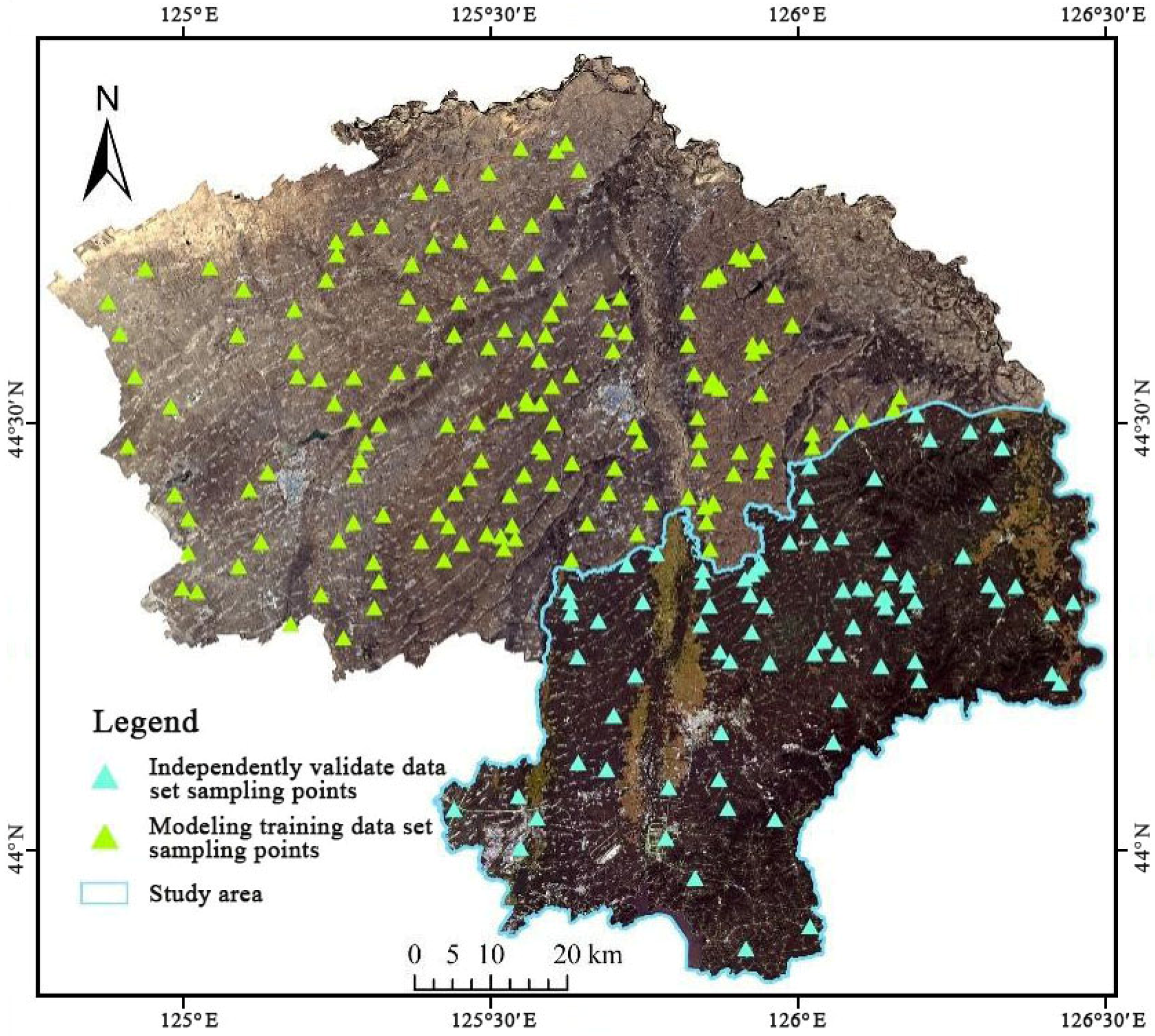
2.1. Study Area, Soil Sampling and Analysis

Jiutai County of Changchun City is located in typical low mountain and hilly terrain, roughly between 43°50′ N–44° 31′ N latitude and 125°24′ E–126°29′ E longitude. The coverage area of Jiutai County has reached about 3 km² and belongs to the monsoon climate zone. The soil in the study site is classified as Mollisols with a texture of clay loam (USDA, Taxonomy).

As the SOC data used in the calculation of the soil erodibility factor in the RUSLE model used in this paper were obtained through remote sensing inversion, to ensure accuracy, the collection range of soil samples was expanded (Figure 1). A total of 240 soil plots were collected by a shovel with depths of 0–30 cm. At each sampling plot within a radius of 2 m, five sites, four sampling points at the corners, and one sampling point at the center of the sampling plot, were selected. The soil samples within the five sampling sites were mixed and placed in a sealed plastic bag to indicate the soil properties of each plot while the spatial coordinates of the plot center were recorded in GPS (Garmin Etrex32X, Bern, Switzerland).

The collected soil samples were dried continuously in an oven at 60 °C for 72 h until constant weight and ground through a 2 mm sieve. The next steps were removing the plant roots and other substances from the sample and further grinding it through a 100 µm screen to determine the SOC content. The determination method of the total carbon content of the soil samples was the dry firing method using a VarioMax CN analyzer (Elementar GmbH, Berlin, Germany). For the soil samples with evident reactions under the treatment of 10% HCl solution, the inorganic carbon content was determined by the pressure calcium meter method. Finally, the SOC content was obtained by subtracting the inorganic carbon content from the total carbon content.

2.2. Data Sources

The Sentinel-2 (S2) remote sensing image data used in this paper were from the European Space Agency and the United States Geological Survey website during 2018–2020. L1C multispectral image data with good quality and less than 10% cloud cover were selected and the Sen2Cor plug-in (ESA released to produce L2A data) was used for atmospheric correction to determine the range of bare cultivated land and SOC inversion. A seamless mosaic tool was employed to merge the multispectral images through Environment for Visualizing Images software. The NDVI is utilized in numerous studies due to its simple estimation, easy availability, and cancellation of noise that is caused due to solar angle, topographic illumination, and clouds [26,27,28]. In this paper, the normalized difference vegetation index (NDVI) was computed by the S2 remote sensing image dataset established above to represent the vegetation cover condition.

NDVI = (Band8 − Band4)/(Band8 + Band4)

(1)

The time node representing 2019 was selected to calculate the erosion triggering factors and amounts of soil erosion. The rainfall from 1986 to 2015 was provided by WorldClim with a spatial resolution of 5 km. Soil texture data were obtained from the 250 m × 250 m rasterized SoilGrids dataset with soil depths of 0–30 cm. The soil data at depths of 0–30 cm were estimated via the weighted depth average method. To determine the terrain factor in the RUSLE model, ALOS DEM data, which have a spatial resolution of 30 m and are derived from NASA EARTHDATA, were selected. On this basis, topographic raster data such as slope gradient, slope length, and slope aspect in the study area were obtained by QGIS 3.10 software.

Based on the first national detailed land survey in 1996 and the unified land survey database in 2019, the land use maps were visually interpreted by using the images from the United States Geological Survey. The accuracy of land use classification was above 90%, and the Kappa coefficient was approximately 0.85. The land use data of the above two years provided the basis for social and economic data, such as the proportion of residential area and road network density, and land use conditions, such as land use intensity and land use landscape fragmentation in the GWR model. The land use intensity mentioned above refers to the efficiency of land resource utilization. In this paper, land use intensity was quantitatively described as four different grades according to land use types (

Table 1. Land use intensity assignment of different land use types.

Land Use Types	Unused Land	Forest, Grassland and Water	Arable Land	Construction Land
Land use intensity grading index	1	2	3	4

In this paper, “construction land” refers to the land used for building buildings, structures, land as a production base, and living place.

). Considering the possibility of multiple land use types distributed in the same grid cell, multiple values of land use intensity are in the same grid cell. Therefore, the land use intensity analysis model should be adopted to calculate the comprehensive land use intensity index of the grid cell as follows:

$$Q_j=100\times \left({\displaystyle \sum }_{i=1}^n{q}_i\times p_i\right)$$

(2)

where $Q_j$ refers to the comprehensive index of land use intensity of the jth grid unit, n is the number of land use intensity grading, $q_i$ refers to the Grade I land use intensity index in the grid unit, and $p_i$ is the ratio of the Grade I land use intensity to the total area of the grid.

Landscape fragmentation is an index of landscape fragmentation in the landscape pattern index, which can reflect the complexity of landscape spatial structure and the degree of human interference to the landscape to a certain extent. In this paper, patch density, edge density, and aggregation index were calculated by Fragstats 4.2 software. The comprehensive index of cultivated land landscape fragmentation degree was obtained after the weight of three indices was calculated by the analytic hierarchy process.

2.3. RUSLE Model

RUSLE, which has been widely applied in multiple previous studies [29,30,31], is a statistical relationship model for predicting the amount of soil erosion, which can correlate the amount of soil erosion and its influencing factors (such as climate condition, soil properties, topography conditions, vegetation cover, and human activities), and can be flexibly modified in terms of the local conditions of influencing factors [32]. Five factors are used in the RUSLE model to estimate the annual average soil loss [33] as follows:

A = R × K × LS ×C × P

(3)

where A indicates the annual average soil erosion modulus (t hm⁻² a⁻¹), R is the rainfall erosivity factor (MJ mm hm⁻² h⁻¹ a⁻¹) linked to the amount of rainfall, and K is the soil erodibility factor (t hm² h hm⁻² MJ⁻¹ mm⁻¹), which is closely related to soil properties. L and S are the slope length and the slope gradient factor, respectively, C is the vegetation cover management factor, and P is the erosion control practice factor. Many researchers in the Northeast Black Soil Region have established local applicable methods for calculating the factors of the RUSLE model [34,35].

2.3.1. Rainfall Erosivity Factor (R)

R characterizes the source power of the rain to create erosion. R was calculated using the method of Zhang and Fu (2003) [36], which is defined using daily rainfall data as follows:

$$R=\epsilon X^{\alpha }$$

(4)

where R indicates the mean rainfall erosivity factor (MJ mm hm^–2 h^–1 a^–1); X indicates the average annual rainfall (mm); ε and α are model parameters, ε = 0.0668, α = 1.6266; and the determination coefficient is 0.828.

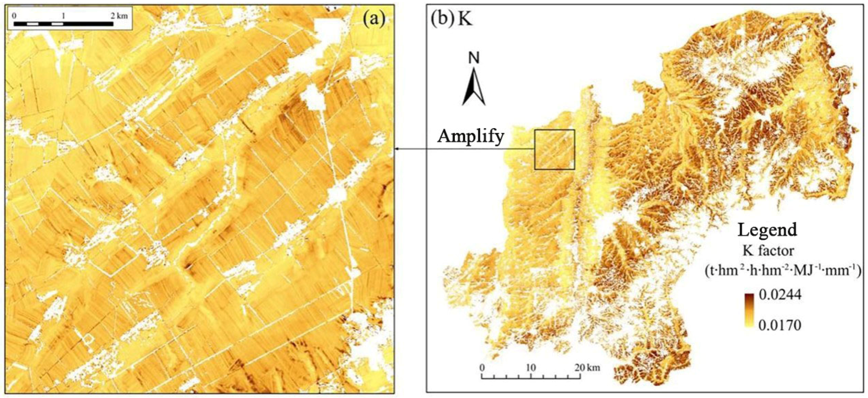
2.3.2. Soil Erodibility Factor (K)

K represents the soil vulnerability to erosion, which indicates the soil sensitivity to denudation separated under raindrop splash, fluctuation, and transportation by runoff. K is sensitive to the texture, structure, OC, hydraulic properties, and wettability of the soil. Many methods for calculating K are available, but the most generally used is the EPIC model based on the soil texture and SOC data [37,38,39]:

$$K=\left\{0.2+0.3exp\left[-0.0256SAN\frac{1-SIL}{100}\right]\right\}\times {\left(\frac{SIL}{CLA+SIL}\right)}^{0.3}\times \left(1-\frac{0.25C}{C+exp(3.72-2.95C}\right)\times \left(1-\frac{0.7S_{n1}}{S_{n1}+exp(-5.51+22.9S_{n1}}\right)$$

(5)

where SAN, SIL, and CLA indicate the sand (0.05–2.0 mm), silt (0.002–0.05 mm), and clay (<0.002 mm) contents (%), respectively, and C is the SOC content (%), $S_{n1}=1-SAN/100$. By multiplying by the coefficient 0.1317, K can be expressed as an SI metric (t hm² h hm⁻² MJ⁻¹ mm⁻¹).

SOC data: S2 remote sensing image data during 2018–2020 were used to construct the bare cropland SOC inversion model. Ten bands covering visible bands (Band2, Band3, and Band4), red-side bands (Band5, Band6, and Band7), near-infrared bands (Band8, Band8A), and shortwave infrared bands (Band11, Band12) were used as an explanatory variable for SOC prediction. The SOC data were the dependent variable in spectral modeling. Coordinate information was used to link soil SOC data from sampling sites with remote sensing spectral information. Model calibration and validation were carried out in R 4.0.3. To evaluate the uncertainty of SOC prediction, different datasets were used for model calibration and cross-validation in 100 repeated simulations. The coefficient of determination (R²) and root mean square error (RMSE) of the measured and predicted values were used to evaluate the performance of the model.

2.3.3. Slope Length and Steepness Factor (LS)

LS is an acceleration factor that reflects the effects of slope length and slope gradient on soil erosion. The estimation method proposed by McCool (1989) [40] and Liu et al., 1994 [41] was comprehensively adopted and applied in the black soil area of Northeast China. The calculation formula is as follows:

$$S=\left\{\begin{array}{c}10.8sin\theta +0.03, \theta <5°\hfill \\ 16.8sin\theta -0.5, 5°\le \theta \le 10°\hfill \\ 21.9sin\theta -0.96, \theta >10°\hfill \end{array}\right.$$

(6)

where θ denotes the slope angle (°).

$$L={\left(\frac{\lambda }{22.13}\right)}^m$$

(7)

$$m=\left\{\begin{array}{c}0.2, \theta \le 0.5°\hfill \\ 0.3, 0.5°<\theta \le 1.5°\hfill \\ 0.4, 1.5°<\theta \le 2.5°\hfill \\ 0.5, \theta >2.5°\hfill \end{array}\right.$$

(8)

where m and λ are the slope length index and the slope length (m), respectively. Among them, 22.13 is the slope length of the standard plot. The LS factors were calculated by the DEM data, and the specific calculation process was achieved by using ArcGIS 10.3 software.

2.3.4. Cover and Management Factor (C)

C represents the erosion control ability of different surface cover types [42]. In the RUSLE model, C is calculated from various subfactors, namely, prior land use, canopy cover, surface cover, surface roughness, and soil moisture [43]. In this paper, the following calculation method was selected for estimating C factor using vegetation cover value [44]:

$$V=\frac{NDVI-NDV{I}_{min}}{NDV{I}_{max}+NDV{I}_{min}}$$

(9)

$$\left\{\begin{array}{c}C=1,0\le V\le 0.001\\ C=0.6508-0.34361\log V,0.001<V\le 0.783\\ C=0,V>0.783\end{array}\right.$$

(10)

where V is the vegetation cover, calculated by retrieval NDVIs derived from the S2 images; NDVI_max is the maximum value (NDVI value of pure vegetation pixel), and NDVI_min is the minimum value (NDVI value of pure bare soil pixel).

2.3.5. Support Practice Factor (P)

P represents an inhibiting factor that reflects the effects of support practices (such as terracing and contour tillage) on soil erosion [45]. Based on previous research results and the actual situation of the research area, the p value of the whole research area was set to 1 in this paper.

2.4. GWR Model

First, before regression weighted analysis, the need for soil erosion risk research and land use factor analysis were considered, and spatial grid units were taken as the basic unit of the study to achieve the purpose of information space statistics. Now, the whole research area was divided into 3 km × 3 km grid cells, and each grid cell was assigned a unique identifier, totaling 445 spatial grid cells.

GWR analysis was first presented by Brunsdon [46] and has been widely used by society and natural scientists [47,48,49]. The GWR model has been mostly applied in urban planning [47,50], environmental science studies [49], geological and geographical remote sensing [51], agricultural sciences [52], and geosciences in some cases [53].

GWR offers better spatial variation as a local function among dependent and independent variables compared with OLSR as a general trend in the entire study area. The general GWR is defined by the following equation [46]:

$$Z_i={\alpha }_0\left(x_i,y_i\right)+{{\displaystyle \sum }}_{k=1}^p{\alpha }_k\left(x_i,y_i\right)w_{ik}+{\epsilon }_{i}i=1,2,\text{…},n$$

(11)

In this paper, Z_i is the explained variable and represents the soil erosion risk index of the ith grid unit. The coordinate of the target region i is $\left(x_i,y_i\right)$, which represents the coordinate of the center point of the ith grid cell. ${\mathsf{\alpha }}_0\left(x_i,y_i\right)$ is the intercept term, K is the explanatory variables value, and ${\mathsf{\alpha }}_k\left(x_i,y_i\right)$ is the first K regression parameter of the ith sampling point and represents the regression parameter of the ith grid cell. $w_{ik}$ is the observed value of explanatory variable $w_k$ at position $\left(x_i,y_i\right)$, ${\mathsf{\epsilon }}_i$ is the random error of the ith sampling point.

In the GWR model, the calculation of the spatial weight matrix is the core content, which represents the spatial dependence of data. The calculation of the weight matrix is closely related to the type and bandwidth of the kernel function. In this paper, Bi-Square function, which has more computational advantage when facing regression analysis with a high degree of data dispersion, was selected. The calculation formula is as follows:

$${\mathrm{W}}_{ij}=e^{\frac{{\left(d_{ij}/b\right)}^2}{2}}$$

(12)

$${\mathrm{W}}_{ij}=\left\{\begin{array}{c}{\left(1-{\left(d_{ij}/b\right)}^2\right)}^2\\ 0, d_{ij}>b\end{array}\right.,d_{ij}\le b$$

(13)

where b is the bandwidth, that is, the parameter for calculating the weight value based on the spatial distance; $d_{ij}$ is the actual spatial distance between observation point j and sampling point i.

In terms of optimal bandwidth selection, this paper adopted the AIC criterion with a higher optimization degree but a relatively complex calculation compared with the cross-validation method. The calculation formula is as follows:

$${\mathrm{AIC}}_c\left(b\right)=2n\ln \widehat{\sigma }+n\ln 2\pi +n\left(\frac{n+tr\left(S\right)}{n-2-tr\left(S\right)}\right)$$

(14)

where n is the number of sample points; $\widehat{\sigma }$ is the maximum likelihood estimate of the variance of the random error term, $\mathsf{\sigma }=\frac{RSS}{n-tr\left(S\right)}.$ The predicted amount of soil erosion in 2019 was used as the dependent variable with a spatial scale of 3 km × 3 km. The selection of explanatory variables considered the three aspects of nature, social economy, and land use that affect soil erosion. Finally, nine explanatory variables were selected to construct the explanatory index system, namely, elevation (X1), slope (X2), precipitation (X3), SOC content (X4), vegetation coverage (X5), change in the proportion of residential areas (X6), change in road network density (X7), change in land use intensity (X8), and change in landscape fragmentation degree of cropland (X9). X6–X9 indicators indicate the change values, which refer to those change values from 1996 to 2019. The impact of land use intensity and land use landscape fragmentation on the spatial distribution of soil erosion was further studied from the perspective of land use.

In this paper, SPSS 22.0 software was used to conduct preliminary data tests on the nine explanatory variables through the tolerance and variance inflation factor (VIF), and the calculation formula is as follows:

$$VIF=\frac{1}{1-R_i^2}$$

(15)

where $R_i^2$ is the square value of the determination coefficient. The larger the VIF is, the smaller the tolerance between explanatory variables.

3. Results and Discussion

3.1. SOC Inversion Based on Multi-Temporal S2 Remote Sensing Image and Composite Soil Pixels

3.1.1. Determination of the Scope of Bare Cultivated Land

NDVImax and NDVImin composite data were established using S2 remote sensing image series data. To determine the critical threshold of bare soil, the NDVI characteristics of farmland, forest, and construction land were statistically calculated. According to the 2019 land use type map, 2000 validation points were randomly selected from each land use category, and the NDVI values of these sampling points were extracted from the NDVI composite data. For the NDVImin combination, the NDVI value representing farmland was between 0.10 and 0.24, which can be clearly distinguished from the forest area. The NDVImax value of construction land was generally lower than that of farmland and forest. Therefore, “NDVImax > 0.75” excluded the construction land area and the range of bare soil was delimited by combining “NDVImax > 0.75” and “0.10 < NDVImin < 0.24” (Figure 2).

To determine the optimal time window, the first step was to use the planting period of the main crops in the study area determined in the FAO crop calendar. In the second step, according to the investigation of 100 bare croplands in the study area, an NDVI threshold of 0.10–0.24 was set and used to remove green vegetation pixels, which was consistent with the study of Shi et al., 2020 [54]. The third step was that NDVI alone was not sufficient to extract bare land pixels, and the Natural Burn Ratio 2 (NBR2) [55] threshold was used to remove soil pixels contaminated by crop residues. The time evolution map of the NDVI in 2019 was plotted with the 2000 cultivated land sampling points mentioned above. Considering that although a similar NDVI distribution occurred in April and October, corn straw remained in the field after the crop harvest in October, so determining the NBR2 threshold was necessary to remove soil pixels further contaminated by crop residue. By comparing the distribution of NBR2 values in the two periods, the NBR2 threshold of 0.075 was used. Castaldi et al., 2019 showed that an NBR2 value of 0.075 was the most appropriate threshold for building a good SOC prediction model [55]. In addition, a study in northern Germany found that this threshold guaranteed a relatively high bare soil coverage, indicating that the NBR2 = 0.075 threshold was suitable for various environments. The above study proved that NBR2 = 0.075 was practical for removing noise pixels affected by environmental pollution. In this paper, NDVI and NBR2 thresholds were combined to perform the extraction of bare cropland for each single-date data image in a predetermined optimal time window. Then, the processed single-date images were filled into the range of bare farmland, and the multitemporal bare soil composite data were obtained by averaging the reflectance of bare soil repeatedly occurring in each pixel.

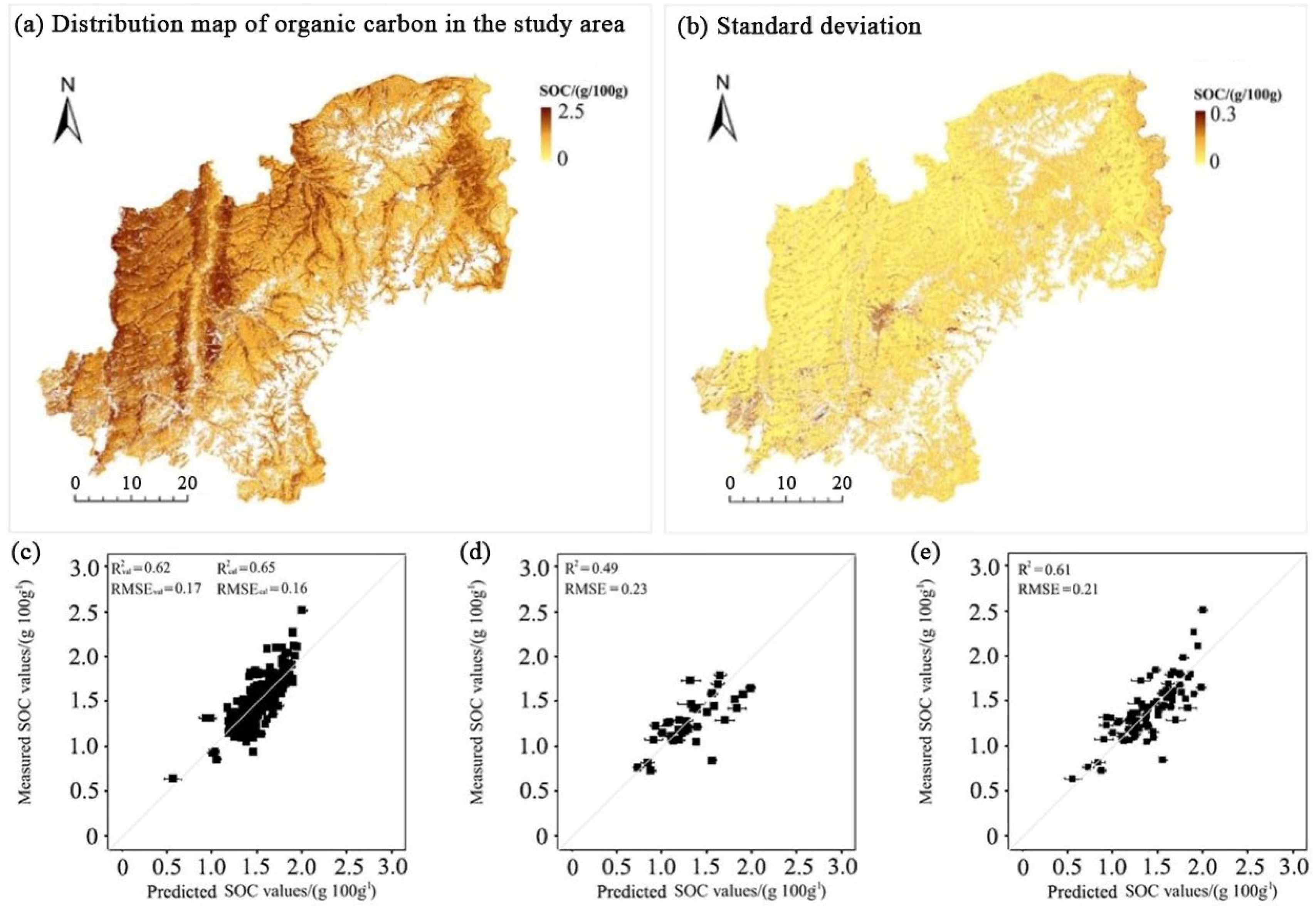
3.1.2. SOC Inversion

A scatter plot was made by a one-to-one correspondence of the “GGplot2” function in R4.0.3 software, as shown in Figure 3. Figure 3c reveals the verification results of the PLSR model based on bare soil composite data developed by the multitemporal S2 remote sensing spectrum improved compared with the PLSR model based on single-date S2 remote sensing data, and the SOC prediction model developed by multitemporal bare soil composite data performed better. R² = 0.53 (2018), 0.59 (2019), and 0.51 (2020) increased to 0.62 (multitemporal), and the RMSE remained almost unchanged. In this paper, the mathematical relationship between spectral information and soil composition was used, but the effects of agricultural activity factors on the modeling effect were ignored, which is also an aspect where further research needs to be improved. Figure 3c,d reveal that compared with the modeling training dataset, the accuracy test results obtained from the independent validation dataset decreased, R² decreased from 0.62 to 0.49, and RMSE increased from 0.17 to 0.23, possibly due to the decreased sample numbers and narrow range of SOC content. Therefore, the prediction results were affected to a certain extent.

A total of 80 soil samples (including 35 independent validation sampling points) were collected in the study area. After evaluating the model performance using the complete soil spectral dataset of 80 groups, Figure 3e shows that the prediction accuracy improved with the increase in the number of sampling points (R² increased from 0.49 to 0.61, RMSE from 0.23 to 0.21). Compared with the best performance evaluation result (R² = 0.32, RMSE = 0.68) in Nascimento et al., 2021 [56] of digital SOC mapping based on remote sensing images, the SOC prediction based on multitemporal S2 remote sensing images in this paper had a more accurate prediction accuracy. Furthermore, the practicability of SOC prediction based on multitemporal remote sensing pixels was illustrated.

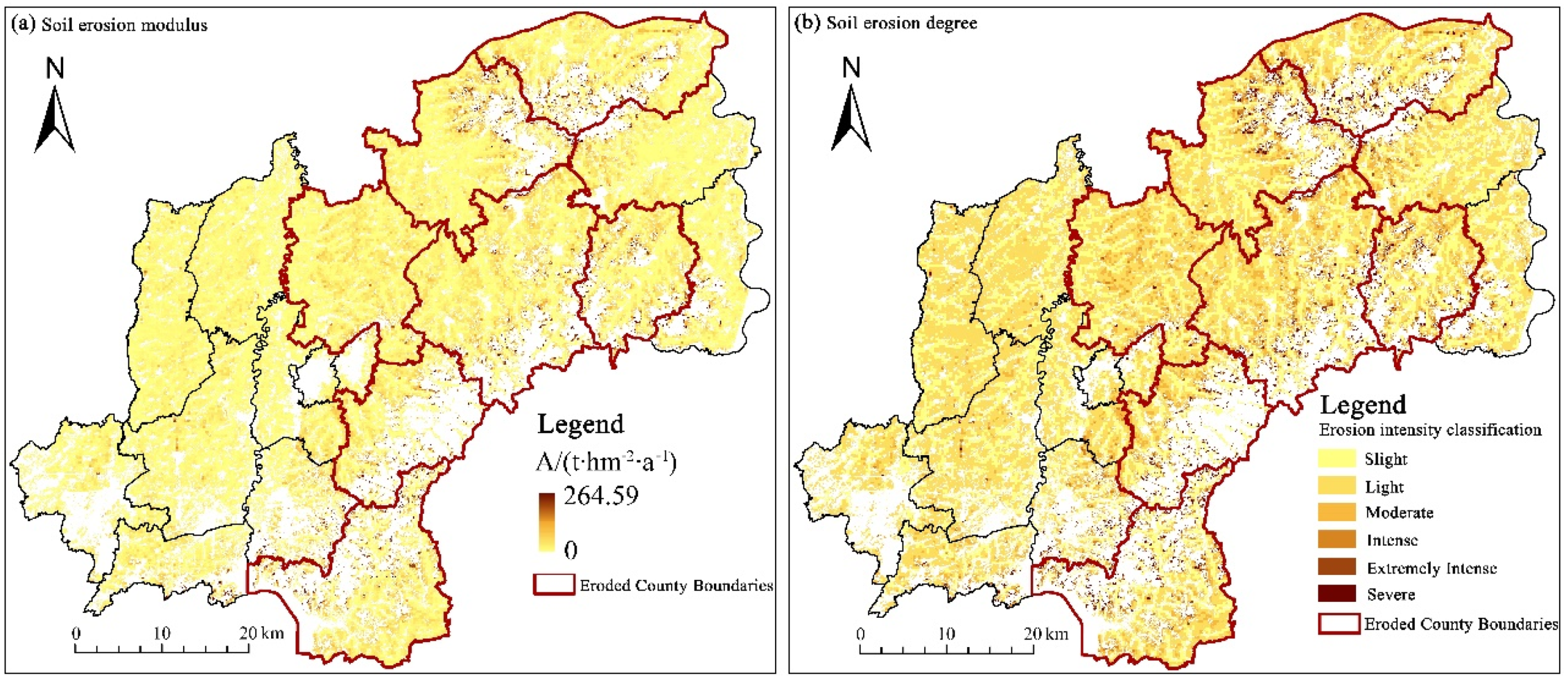
3.2. Spatial Mapping of Soil Erodibility Factor and Soil Erosion Risk

The soil texture was fine, and the calculated value of the soil erodibility factor was small (0.0168–0.0203 t hm² h hm⁻² MJ⁻¹ mm⁻¹). Clearly, the southeastern region of the study area had a higher SOC content and lower predicted results of soil erodibility factors than the northwestern region.

The SOC spatial distribution data based on S2 high-resolution remote sensing images can improve the spatial resolution of the soil erodibility factor map (Figure 4). Based on the amplification effect of the spatial distribution of the K value (Figure 4), the K value calculated by the SOC data inversion based on S2 can reflect the spatial heterogeneity characteristics of the K value, which is important for refining the spatial difference characteristics of soil erosion. Additionally, proper agricultural practices would maintain sufficient SOC and aggregate structures to help control the development of soil erosion [57].

Using the remote sensing inversion techniques, erosion factor calculation equation, and RUSLE model, soil erosion and the interfering factors in the study area in 2019 were assessed and mapped, which provided available information to serve as a primary reference for soil and water conservation management. Based on the soil erosion classification standard in the Technical Standard for Comprehensive Control of Soil and Water Loss in Black Soil Area (SL446-2009) promulgated by the Ministry of Water Resources of China, the soil erosion degree was divided into six grades (

Table 2. Statistical results of different soil erosion intensities of cropland.

Soil Erosion Intensity Grade	Soil Erosion Modulus/ t hm−2 a−1	Area/km2	Proportion of Total Arable Land/%
1. Slight	≤2	697.44	31.99
2. Light	2–12	1117.43	51.25
3. Moderate	12–24	242.93	11.14
4. Intense	24–36	60.70	2.78
5. Extremely Intense	36–48	24.18	1.11
6. Severe	>48	37.51	1.72

and Figure 5). From the size of the area eroded, the soil erosion of bare farmland in the study area was mainly slight and light, which accounted for 31.99% and 51.25% of the total area of cultivated land, respectively. Moderate erosion followed, accounting for 11.14% of the total area of bare cultivated land. The proportion of cultivated land with extremely intense and severe erosion was 2.83%. In terms of spatial distribution, the cropland with serious soil erosion was mainly distributed in the sloping farmland with higher elevation and more gullies (southeastern and northeastern hilly areas). In the flat area (central and western regions) where the river flowed, the soil erosion of cultivated land was light, mainly with slight erosion and light erosion. Soil erosion maps can be used as a basic document for rational land planning to avoid potential water and soil losses effectively. The sloping grasslands in the low mountain and hilly area had a high risk of soil and water loss, which required the implementation of effective management and control measures.

Xu and Zhang (2020) [29] showed that the spatiotemporal characteristics in soil erosion could only be uncovered more accurately by spatially quantifying different change methods of triggering factors and their relative importance. Figure 6 shows that topographic factors have the greatest influence on the spatial distribution of soil erosion, and the spatial distribution of topography factors would help explain the change in soil erosion, so the relationship must be determined. According to statistics, with increasing altitude, the proportion of slight and light soil erosion gradually decreased, while the proportion of extreme intensity and severe erosion gradually increases. With the increase in terrain slope, the proportion of slight and light soil erosion gradually decreased, while the proportion of extreme intensity and severe erosion gradually increases. The most serious soil erosion intensity was concentrated in the southeast and northeast sloping farmland over 8°. Finally, overall, soil erosion on the sunny slope was slightly more serious than that on the shady slope possibly because the sunny slope was the windward slope of the southeast monsoon, and the soil water evaporation was larger than that on the shady slope, resulting in a lower soil water content, which reduced the vegetation coverage and made soil erosion more likely. LS was the leading factor of regional soil erosion. Therefore, better spatial optimal allocation of land use is needed to avoid steep areas prone to erosion [29,58]. Arable land was widely distributed in the flat regions with much lower LS factors than in grasslands and forests. The cultivated land distributed around the forestland faced the soil erosion risk due to the terrain and became unstable cultivated land. When the study area was larger, future soil erosion risk from spatial and temporal changes in precipitation should be considered and evaluated by using the future climate change prediction models. The K at the field scale can be calculated by more accurate soil attribute data, which would be needed in water and soil conversation planning.

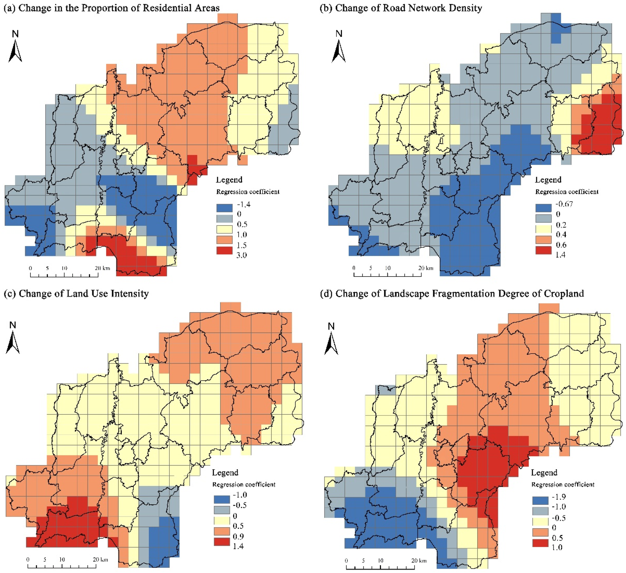
3.3. Land Use Factor Analysis of Cropland Soil Erosion Based on the GWR Model

Table 3. Multicollinearity test results of independent variables.

Type Layer	Explanatory Variables	Collinearity Test Results
		Tolerance	VIF
Natural conditions	Elevation (X1)	0.94	1.07
	Slope (X2)	0.67	1.49
	Precipitation (X3)	0.44	2.27
	SOC content (X4)	0.50	1.99
	Vegetation coverage (X5)	0.79	1.27
Socioeconomic conditions	Change in the proportion of residential areas (X6)	0.92	1.09
	Change of road network density (X7)	0.88	1.14
Land Use conditions	Change of land use intensity (X8)	0.93	1.08
	Change of landscape fragmentation degree of cropland (X9)	0.98	1.02

shows that the VIF of the independent variables was less than 5 and the condition index was less than 30, which proved that the nine explanatory variables selected passed the multicollinearity test.

The preliminary statistics of the regression coefficients of each explanatory variable of soil erosion in the GWR model (

Table 4. Statistical result of regression coefficients of explanatory variables.

Explanatory Variables	Minimum	Upper Quartile	Median	Average	Lower Quartile	Maximum	Standard Deviation
Elevation	−1.89	−0.05	0.08	−0.01	0.20	1.01	0.45
Slope	4.03	5.54	5.94	6.18	6.46	9.04	1.09
Precipitation	−1.76	−0.92	−0.55	−0.56	−0.17	0.63	0.51
SOC content	−2.56	−0.72	−0.47	−0.56	−0.30	0.29	0.49
Vegetation coverage	−0.57	0.06	0.16	0.24	0.41	1.54	0.35
Change in the proportion of residential areas	−1.42	0.17	0.83	0.69	1.19	3.01	0.69
Change in road network density	−0.67	0.00	0.11	0.10	0.20	1.46	0.30
Change of land use intensity	−1.98	−0.68	0.49	0.46	0.62	1.39	0.37
Change of landscape fragmentation degree of cropland	−1.92	−0.37	−0.16	−0.17	0.25	1.04	0.59

) showed that the plus or minus statistical values of the regression coefficients proved the existence of both positive and negative correlations between the explanatory variables and the soil erosion of cultivated land in different grid cells.

Chaplot et al., 2005 [59] found that the influence of land use change on soil erosion is greater than that of climate factors, especially in regard to rill erosion. Simonneaux et al., 2015 [60] showed that the increase in soil erosion caused by land use change is much greater than that caused by climate change in Morocco. Compared with forests, farmland has a lower interception rate, resulting in a higher runoff [61].

In this paper, the changes in the proportion of residential area, road network density, and land use intensity, for which the median and mean regression coefficients were positive, explained that the relationship between the above three indices and the cropland soil erosion degree was positively correlated in most grid cells (Figure 7), that is, the increase in the proportion of residential area had a positive influence on the soil erosion severity. The median and mean values of the regression coefficients of farmland landscape fragmentation change were both negative, indicating that the soil erosion degree of farmland decreased with the increase in the explanatory variables of farmland landscape fragmentation change in most grid cells.

The increase in the proportion of residential area, the intensity of land use, and the fragmentation degree of the cultivated land landscape all had a remarkable impact on the soil erosion pattern of surrounding cultivated land to varying degrees (Figure 7). Among them, the proportion of residential area and the fragmentation degree of the cultivated land landscape had the widest impact on the areas with high erosion risk. Therefore, optimizing the development and protection pattern of territorial space with appropriate land regulation means avoiding the further aggravation of soil erosion is necessary.

An increase in residential areas and land use intensity meant an increase in impermeable surface area. In the construction, a large number of materials, such as cement, asphalt, and concrete, were used to cover the soil surface to form an impermeable surface. According to the research, under the conditions of runoff and precipitation, the runoff coefficient of a completely impermeable surface was more than 0.9, that is, almost all precipitation was transformed into surface runoff. The intensification of surface runoff under rainstorm conditions increased the pressure of urban drainage, and the capacity of drainage pipelines usually had difficulty meeting the discharge of a large amount of surface runoff in a short time, resulting in serious surface ponding, especially in low-lying areas. In the area where the land use degree increased, the proportion of impermeable surfaces increase, resulting in an increase in the overall surface runoff in the area. The degree of soil and water loss was more serious in summer with heavy rainfall because the study area is in the monsoon climate area [12]. Wang et al., 2022 found that compared with the western region of the black soil region, the eastern region where the study area is located has a humid climate, and water is the main erosive agent [62].

The area selected in this study belonged to a rolling hilly region with a small area of suitable cultivated land in low mountain and hilly areas, and the overall uphill cultivated land showed the characteristics of high spatial dispersion. To obtain the minimum survival guarantee, only by continuously expanding the cultivated land area, which leads to more barren mountains that are not suitable for farming being reclaimed into cultivated land, accelerates the dispersion and fragmentation of farming space. Compared with natural factors, the land use factor of cropland encompassed the most easily optimized measures. The degree of landscape fragmentation played a positive role in soil erosion. Therefore, to control soil and water loss, the land use pattern can be optimized by enhancing the control effect of the dominant landscape, improving patch uniformity, enriching landscape types, reducing the physical connection between patches, strengthening the aggregation degree of landscape patches, and reducing fragmentation. On a deeper level, as a typical social dominant area, the low hilly agricultural area should always pay attention to the balance/synergy between social services and ecological functions, so as to lay a foundation for sustainable land use in the black soil area [63].

4. Conclusions

In 2019, the overall soil erosion status of cultivated land was mainly slight and light, the proportion of cultivated land affected by the extreme intensity and severe erosion was relatively small, and the average soil erosion modulus was 7.09 t·hm⁻²·a⁻¹. The spatial distribution characteristics of soil erosion based on the results of spatial aggregation and hot spot analysis found that the most serious soil erosion intensity was concentrated in the southeast and northeast sloping farmland. With the increase in elevation and topographic slope, the proportions of slight and light soil erosion gradually decreased while the proportions of extreme intensity and severe erosion gradually increased, which was strongly linked to the increase of soil erodibility caused by the space-time migration and erosion of SOC caused by the interaction of hydraulic and tillage erosion in complex topographic areas.

Based on the relationship between soil erosion and landscape fragmentation using the GWR model in a rolling hilly region, the findings revealed that landscape fragmentation was an important driving force promoting soil erosion, sediment yield, and sediment transport. On this basis, sloping farmland with a high fragmentation degree was effectively integrated to prevent soil erosion in marginal farmland. The prevention and control of soil erosion in hilly areas should be based on the premise of rational utilization of land resources, and the situation of “governing and destroying at the same time” should be completely changed. The finding of this paper can be used as a basis for decision-making in a rolling hilly region, and provide useful information for designing land use planning to regulate the effect of land use change and other soil erosion factors. Land use planning and water and soil conservation planning should be combined to provide a scientific basis for the sustainable land use of land resources and the coordinated development of man-land relationships in hilly areas.

References

1. Garcia, L.; Celette, F.; Gary, C.; Ripoche, A.; Valdés-Gómez, H.; Metay, A. Management of service crops for the provision of ecosystem services in vineyards: A review. Agric. Ecosyst. Environ. 2018, 251, 158–170. [Google Scholar] [CrossRef]
2. Berhe, A.A.; Barnes, R.T.; Six, J.; Marín-Spiotta, E. Role of soil erosion in biogeochemical cycling of essential elements: Carbon, nitrogen, and phosphorus. Annu. Rev. Earth Planet. Sci. 2018, 46, 521–548. [Google Scholar] [CrossRef]
3. Zhao, H.L.; Yi, X.Y.; Zhou, R.L.; Zhao, X.Y.; Zhang, T.H.; Drake, S. Wind erosion and sand accumulation effects on soil properties in Horqin Sandy Farmland, Inner Mongolia. Catena 2006, 65, 71–79. [Google Scholar] [CrossRef]
4. Quinton, J.N.; Govers, G.; Van Oost, K.; Bardgett, R.D. The impact of agricultural soil erosion on biogeochemical cycling. Nat. Geosci. 2010, 3, 311. [Google Scholar] [CrossRef]
5. Hancock, G.R.; Wells, T. Predicting soil organic carbon movement and concentration using a soil erosion and Landscape Evolution Model. Geoderma 2021, 382, 114759. [Google Scholar] [CrossRef]
6. Müller-Nedebock, D.; Chivenge, P.; Chaplot, V. Selective organic carbon losses from soils by sheet erosion and main controls Earth Surf Process. Landforms 2016, 41, 1399–1408. [Google Scholar] [CrossRef]
7. Pimentel, D.; Harvey, C.; Resosudarmo, P.; Sinclair, K.; Kurz, D.; Mcnair, M.; Crist, S.; Shpritz, L.; Fitton, L.; Saffouri, R. Environmental and Economic Costs of Soil Erosion and Conservation Benefits. Science 1995, 267, 1117–1123. [Google Scholar] [CrossRef]
8. Chappell, A.; Baldock, J.; Sanderman, J. The global significance of omitting soil erosion from soil organic carbon cycling schemes. Nat. Clim. Change 2016, 6, 187–191. [Google Scholar] [CrossRef]
9. Wang, Z.J.; Jiao, J.Y.; Rayburg, S.; Wang, Q.L.; Su, Y. Soil erosion resistance of “Grain for Green” vegetation types under extreme rainfall conditions on the Loess Plateau, China. Catena 2016, 141, 109–116. [Google Scholar] [CrossRef]
10. Yue, Y.; Ni, J.R.; Ciais, P.; Piao, S.L.; Wang, T.; Huang, M.T.; Li, T.H.; Wang, Y.C.; Chappell, A.; Van Oost, K. Lateral transport of soil carbon and land-atmosphere CO2 flux induced by water erosion in China. Proc. Natl. Acad. Sci. USA 2016, 113, 6617–6622. [Google Scholar] [CrossRef]
11. Liu, B.; Xie, Y.; Li, Z.; Liang, Y.; Guo, Q. The assessment of soil loss by water erosion in China. Int. Soil Water Conserv. Res. 2020, 8, 430–439. [Google Scholar] [CrossRef]
12. Wan, W.; Liu, Z.; Li, B.G.; Fang, H.Y.; Wu, H.Q.; Yang, H.Y. Evaluating soil erosion by introducing crop residue cover and anthropogenic disturbance intensity into cropland C-factor calculation: Novel estimations from a cropland-dominant region of Northeast China. Soil Tillage Res. 2022, 219, 105434. [Google Scholar] [CrossRef]
13. Chen, L.; Wang, J.; Fu, B.; Qiu, Y. Land-use change in a small catchment of northern Loess Plateau, China. Agric. Ecosyst. Environ. 2001, 86, 163–172. [Google Scholar] [CrossRef]
14. Alem, B.B. The nexus between land use land cover dynamics and soil erosion hotspot area of Girana Watershed, Awash Basin, Ethiopia. Heliyon 2022, 8, e08916. [Google Scholar] [CrossRef]
15. Bagarello, V.; Di Stefano, V.; Ferro, V.; Giordano, G.; Iovino, M.; Pampalone, V. Estimating the USLE Soil Erodibility Factor in Sicily, South Italy. Trop. Agric. 2012, 28, 199–206. [Google Scholar] [CrossRef]
16. Klein, J.; Jarva, J.; Frank-Kamenetsky, D.; Bogatyrev, I. Integrated geological risk mapping: A qualitative methodology applied in St. Petersburg, Russia. Environ. Earth Sci. 2013, 70, 1629–1645. [Google Scholar] [CrossRef]
17. Adhikary, P.P.; Tiwari, S.P.; Mandal, D.; Lakaria, B.L.; Madhu, M. Geospatial comparison of four models to predict soil erodibility in a semi-arid region of Central India. Environ. Earth Sci. 2014, 72, 5049–5062. [Google Scholar] [CrossRef]
18. Garcia-Ruiz, J.M.; Begueria, S.; Nadal-Romero, E.; González-Hidalgo, J.C.; Lana-Renault, N.; Sanjuán, Y. A meta-analysis of soil erosion rates across the world. Geomorphology 2015, 239, 160–173. [Google Scholar] [CrossRef]
19. Zare, M.; Panagopoulos, T.; Loures, L. Simulating the impacts of future land use change on soil erosion in the Kasilian watershed. Land Use Policy 2017, 67, 558–572. [Google Scholar] [CrossRef]
20. Liu, X.; Burras, C.L.; Kravchenko, Y.S.; Duran, A.; Huffman, T.; Morras, H.; Yuan, X. Overview of Mollisols in the world: Distribution, land use and management. Can. J. Soil Sci. 2012, 92, 383–402. [Google Scholar] [CrossRef]
21. Liu, X.; Zhang, S.; Zhang, X.; Ding, G.; Cruse, R.M. Soil erosion control practices in Northeast China: A mini-review. Soil Tillage Res. 2012, 117, 44–48. [Google Scholar] [CrossRef]
22. Todd-Brown, K.E.O.; Randerson, J.T.; Hopkins, F.; Arora, V.; Hajima, T.; Jones, C.; Zhang, Q. Changes in soil organic carbon storage predicted by Earth system models during the 21st century. Biogeosciences 2014, 11, 2341–2356. [Google Scholar] [CrossRef]
23. Li, H.; Liao, X.; Zhu, H.; Wei, X.; Shao, M. Soil physical and hydraulic properties under different land uses in the black soil region of Northeast China. Can. J. Soil Sci. 2019, 99, 406–419. [Google Scholar] [CrossRef]
24. Duan, X.; Xie, Y.; Ou, T.; Lu, H. Effects of soil erosion on long-term soil productivity in the black soil region of northeastern China. Catena 2011, 87, 268–275. [Google Scholar] [CrossRef]
25. Yu, Z.; Wang, G.; Jin, J.; Liu, J.; Liu, X. Soil microbial communities are affected more by land use than seasonal variation in restored grassland and cultivated Mollisols in Northeast China. Eur. J. Soil Biol. 2011, 47, 357–363. [Google Scholar] [CrossRef]
26. Kumari, N.N.; Srivastava, A.; Dumka, U.C. A Long-Term Spatiotemporal Analysis of Vegetation Greenness over the Himalayan Region Using Google Earth Engine. Climate 2021, 9, 109. [Google Scholar] [CrossRef]
27. Matsushita, B.; Yang, W.; Chen, J.; Onda, Y.; Qiu, G. Sensitivity of the enhanced vegetation index (EVI) and normalized difference vegetation index (NDVI) to topographic effects: A case study in high-density cypress forest. Sensors 2007, 7, 2636–2651. [Google Scholar] [CrossRef]
28. Pei, F.S.; Zhou, Y.; Xia, Y. Application of Normalized Difference Vegetation Index (NDVI) for the Detection of Extreme Precipitation Change. Forest 2021, 12, 594. [Google Scholar] [CrossRef]
29. Xu, E.Q.; Zhang, H.Q. Change pathway and intersection of rainfall, soil, and land use influencing water-related soil erosion. Ecol. Indic. 2020, 113, 106281. [Google Scholar] [CrossRef]
30. Hu, T.; Wu, J.S.; Li, W.F. Assessing relationships of ecosystem services on multiscale: A case study of soil erosion control and water yield in the Pearl River Delta. Ecol. Ind. 2019, 99, 193–202. [Google Scholar] [CrossRef]
31. Zeng, C.; Wang, S.; Bai, X.; Li, Y.; Tian, Y.; Li, Y.; Wu, L.; Luo, G. Soil erosion evolution and spatial correlation analysis in a typical karst geomorphology using RUSLE with GIS. Solid Earth 2017, 8, 721–736. [Google Scholar] [CrossRef]
32. Sun, W.Y.; Shao, Q.Q.; Liu, J.Y.; Zhai, J. Assessing the effects of land use and topography on soil erosion on the Loess Plateau in China. Catena 2014, 121, 151–163. [Google Scholar] [CrossRef]
33. Renard, K.G.; Foster, G.R.; Weesies, G.A.; McCool, D.K.; Yoder, D.C. Predicting Soil Erosion by Water: A Guide to Conservation Planning with the Revised Universal Soil Loss Equation (RUSLE); United States Department of Agriculture: Washington, DC, USA, 1997. [Google Scholar]
34. Tang, Q.; Xu, Y.; Bennett, S.J.; Li, Y. Assessment of soil erosion using RUSLE and GIS: A case study of the Yangou watershed in the Loess Plateau, China. Environ. Earth Sci. 2015, 73, 1715–1724. [Google Scholar] [CrossRef]
35. Li, P.F.; Zang, Y.Z.; Ma, D.D.; Yao, W.Q.; Holden, J.; Irvine, B.; Zhao, G.J. Soil erosion rates assessed by RUSLE and PESERA for a Chinese Loess Plateau catchment under land-cover changes. Earth Surf. Proc. Land 2020, 45, 707–722. [Google Scholar] [CrossRef]
36. Zhang, W.B.; Fu, J.S. Rainfall erosivity estimation under different rainfall amount. Resour. Sci. 2003, 25, 35–41. [Google Scholar]
37. Sharpley, A.N.; Williams, J.R. EPIC–Erosion/Productivity Impact Calculator: 1. Model Documentation; USDA Technical Bulletin No. 1768; USDA: Washington, DC, USA, 1990. [Google Scholar]
38. Zhang, K.L.; Shu, A.P.; Xu, X.L.; Yang, Q.K.; Yu, B. Soil erodibility and its estimation for agricultural soils in China. J. Arid Environ. 2008, 72, 1002–1011. [Google Scholar] [CrossRef]
39. Huang, X.F.; Lin, L.R.; Ding, S.W.; Tian, Z.C.; Zhu, X.Y.; Wu, K.R.; Zhao, Y.Z. Characteristics of Soil Erodibility K Value and Its Influencing Factors in the Changyan Watershed, Southwest Hubei, China. Land 2022, 11, 134. [Google Scholar] [CrossRef]
40. McCool, D.K.; Foster, G.R.; Mutchler, C.K.; Meyer, L.D. Revised slope length factor for the universal soil loss equation. Trans. ASAE 1989, 32, 1571–1576. [Google Scholar] [CrossRef]
41. Liu, B.Y.; Nearing, M.A.; Risse, L.M. Slope gradient effects on soil loss for steep slopes. Trans. ASAE 1994, 37, 1835–1840. [Google Scholar] [CrossRef]
42. Guerra, C.A.; Maes, J.; Geijzendorffer, I.; Metzger, M.J. An assessment of soil erosion prevention by vegetation in Mediterranean Europe: Current trends of ecosystem service provision. Ecol. Ind. 2016, 60, 213–222. [Google Scholar] [CrossRef]
43. Tanyas, H.; Kolat, C.; Süzen, M.L. A new approach to estimate cover-management factor of RUSLE and validation of RUSLE model in the watershed of Kartalkaya Dam. J. Hydrol. 2015, 528, 584–598. [Google Scholar] [CrossRef]
44. Cai, C.; Ding, S.; Shi, Z.; Huang, L.; Zhang, G. Study of applying USLE and geographical information system IDRISI to predict soil erosion in small watershed. J. Soil Water Conserv. 2000, 14, 19–24. (In Chinese) [Google Scholar]
45. Phinzi, K.; Ngetar, N.S. The assessment of water-borne erosion at catchment level using GIS-based RUSLE and remote sensing: A review. Int. Soil Water Conserv. Res. 2019, 7, 27–46. [Google Scholar] [CrossRef]
46. Brunsdon, C.; Fotheringham, S.; Charlton, M. Geographically weighted regression. J. R. Stat. Soc. Ser. D 1998, 47, 431–443. [Google Scholar] [CrossRef]
47. Huang, J.; Huang, Y.; Pontius, R.G.; Zhang, Z. Geographically weighted regression to measure spatial variations in correlations between water pollution versus land use in a coastal watershed. Ocean Coast. Manag. 2015, 103, 14–24. [Google Scholar] [CrossRef]
48. See, L.; Schepaschenko, D.; Lesiv, M.; McCallum, I.; Fritz, S.; Comber, A.; Perger, C.; Schill, C.; Zhao, Y.; Maus, V. Building a hybrid land cover map with crowdsourcing and geographically weighted regression. ISPRS J. Photogramm. Remote Sens. 2015, 103, 48–56. [Google Scholar] [CrossRef]
49. Wu, S.S.; Yang, H.; Guo, F.; Han, R.M. Spatial patterns and origins of heavy metals in Sheyang River catchment in Jiangsu, China based on geographically weighted regression. Sci. Total Environ. 2017, 580, 1518–1529. [Google Scholar] [CrossRef]
50. Gao, J.; Li, S. Detecting spatially non-stationary and scale-dependent relationships between urban landscape fragmentation and related factors using geographically weighted regression. Appl. Geogr. 2011, 31, 292–302. [Google Scholar] [CrossRef]
51. Song, W.; Jia, H.; Huang, J.; Zhang, Y. A satellite-based geographically weighted regression model for regional PM 2.5 estimation over the Pearl River Delta region in China. Remote Sens. Environ. 2014, 154, 1–7. [Google Scholar] [CrossRef]
52. Zhang, C.; Tang, Y.; Xu, X.; Kiely, G. Towards spatial geochemical modelling: Use of geographically weighted regression for mapping soil organic carbon contents in Ireland. Appl. Geochem. 2011, 26, 1239–1248. [Google Scholar] [CrossRef]
53. Zhao, J.; Wang, W.; Cheng, Q. Application of geographically weighted regression to identify spatially non-stationary relationships between Fe mineralization and its controlling factors in eastern Tianshan, China. Ore Geol. Rev. 2014, 57, 628–638. [Google Scholar] [CrossRef]
54. Shi, P.; Castaldi, F.; van Wesemael, B.; Van Oosta, K. Vis-NIR spectroscopic assessment of soil aggregate stability and aggregate size distribution in the Belgian Loam Belt. Remote Sens. 2020, 12, 666. [Google Scholar] [CrossRef]
55. Castaldi, F.; Hueni, A.; Chabrillat, S.; Ward, K.; Buttafuoco, G.; Bomans, B.; Vreys, K.; Brell, M.; van Wesemael, B. Evaluating the capability of the Sentinel 2 data for soil organic carbon prediction in croplands. ISPRS J. Photogramm. 2019, 147, 267–282. [Google Scholar] [CrossRef]
56. Nascimento, C.M.; Mendes, W.D.S.; Silvero, N.E.Q.; Poppiel, R.R.; Sayão, V.M.; Dotto, A.C.; dos Santos, N.V.; Accorsi, M.T.; Demattê, J.A.M. Soil degradation index developed by multitemporal remote sensing images, climate variables, terrain and soil atributes. J. Environ. Manag. 2021, 277, 111316. [Google Scholar] [CrossRef]
57. Pimentel, D. Soil Erosion: A Food and Environmental Threat. Environ. Dev. Sustain. 2006, 8, 119–137. [Google Scholar] [CrossRef]
58. Sadeghi, S.H.R.; Jalili, K.; Nikkami, D. Land use optimization in watershed scale. Land Use Policy 2009, 26, 186–193. [Google Scholar] [CrossRef]
59. Chaplot, V.; Giboire, G.; Marchand, P.; Valentin, C. Dynamic modelling for linear erosion initiation and development under climate and land-use changes in northern Laos. Catena 2005, 63, 318–328. [Google Scholar] [CrossRef]
60. Simonneaux, V.; Cheggour, A.; Deschamps, C.; Mouillot, F.; Cerdan, O.; Le Bissonnais, Y. Land use and climate change effects on soil erosion in a semi-arid mountainous watershed (High Atlas, Morocco). J. Arid Environ. 2015, 122, 64–75. [Google Scholar] [CrossRef]
61. Fohrer, N.; Haverkamp, S.; Eckhardt, K.; Frede, H.G. Hydrologic Response to land use changes on the catchment scale. Phys. Chem. Earth B—Hydrol. Oceans Atmos. 2001, 26, 577–582. [Google Scholar] [CrossRef]
62. Wang, H.; Yang, S.L.; Wang, Y.D.; Gu, Z.Y.; Xiong, S.F.; Huang, X.F.; Sun, M.M.; Zhang, S.H.; Guo, L.C.; Cui, J.Y.; et al. Rates and causes of black soil erosion in Northeast China. Catena 2022, 214, 106250. [Google Scholar] [CrossRef]
63. Zhang, Y.N.; Long, H.L.; Tu, S.S.; Ge, D.Z.; Ma, L.; Wang, L.Z. Spatial identification of land use functions and their tradeoffs/synergies in China: Implications for sustainable land management. Ecol. Indic. 2019, 107, 105550. [Google Scholar] [CrossRef]
Figure 1. Distribution map of sampling points.
Land 11 01253 g001
Figure 2. Spatial distribution of bare cultivated land in the study area. (a) map is the effect diagram of bare cultivated land identification in part of (b) map.
Land 11 01253 g002
Figure 3. PLSR model validation results and spatial distribution of SOC based on multi-temporal S2 remote sensing spectral data set. (a) Spatial distribution map of SOC; (b) Spatial distribution of standard deviation of SOC; PLSR model validation results based on (c) modeling training data sets; (d) independent validation data sets; (e) the complete data set.
Land 11 01253 g003
Figure 4. Spatial distribution of soil erodibility factors in the study area. (a) map shows the magnified effect of the local area of (b) map.
Land 11 01253 g004
Figure 5. Spatial distribution of soil erosion modulus (a) and intensity grade (b) in the study area.
Land 11 01253 g005
Figure 6. Proportion of soil erosion grades of cultivated land at different altitudes, slopes, and aspects.
Land 11 01253 g006
Figure 7. Spatial distribution of regression coefficients of explanatory variables of socioeconomic and land use factors in the GWR model.
Land 11 01253 g007