
Evaluating Ecosystem Services and Trade-Offs Based on Land-Use Simulation: A Case Study in the Farming–Pastoral Ecotone of Northern China

 , ,
, , 
 and
and
Abstract
:1. Introduction
2. Materials and Methods
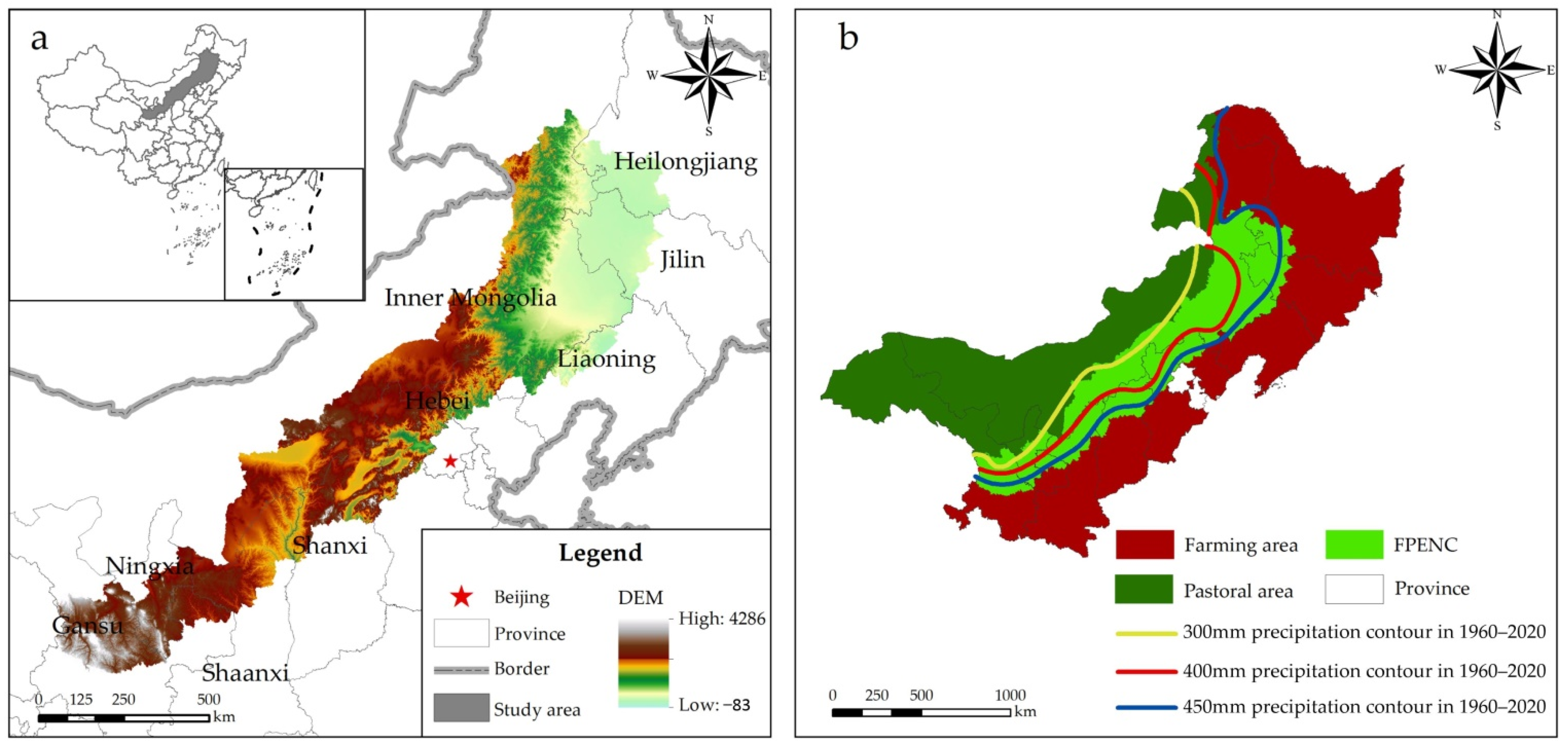
2.1. Study Area
2.2. Data Sources
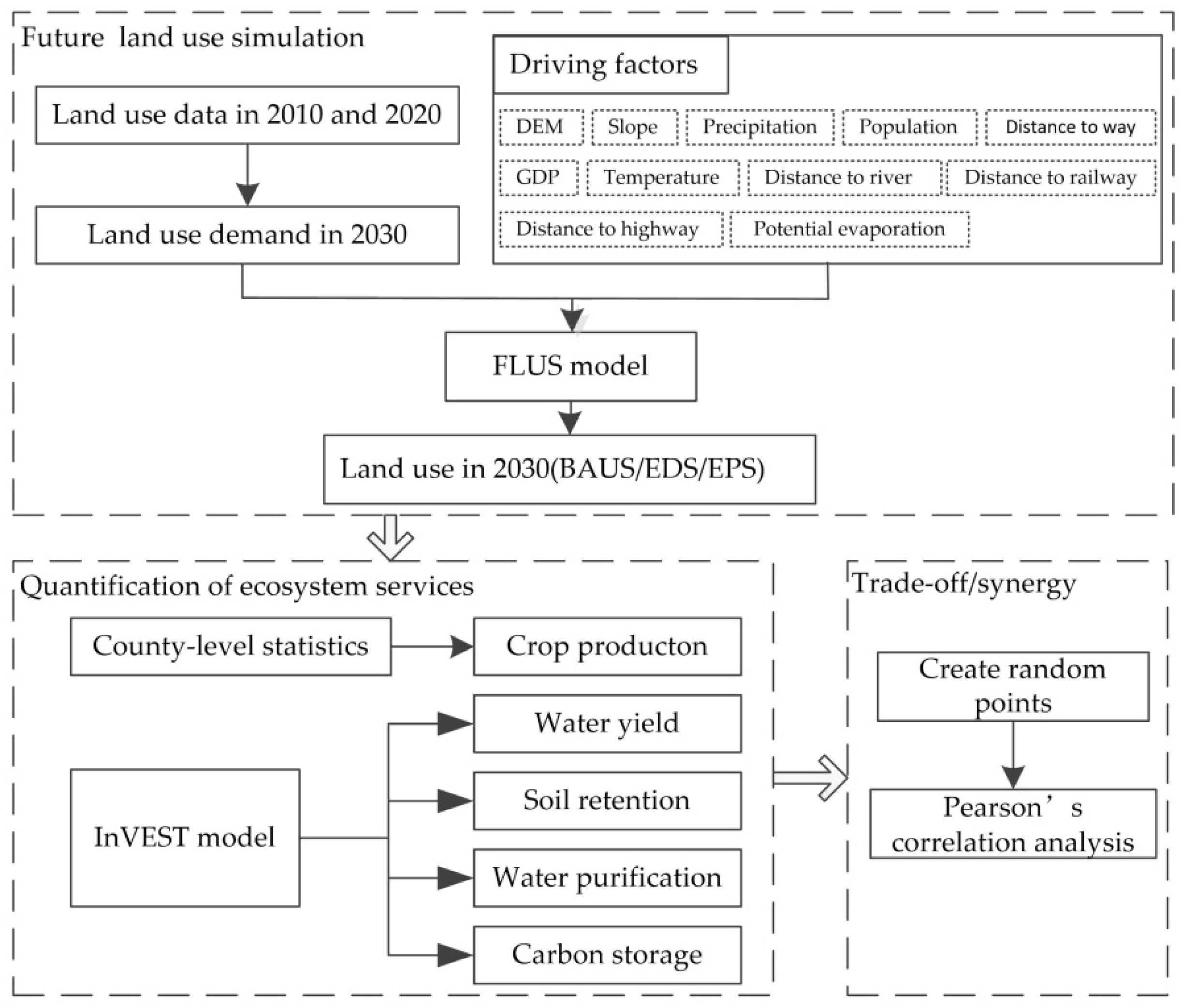
2.3. Framework
2.3.1. FLUS Model
2.3.2. Scenarios Setting
2.3.3. Quantification of Ecosystem Services (ESs)
2.3.4. Statistical Analysis
3. Results
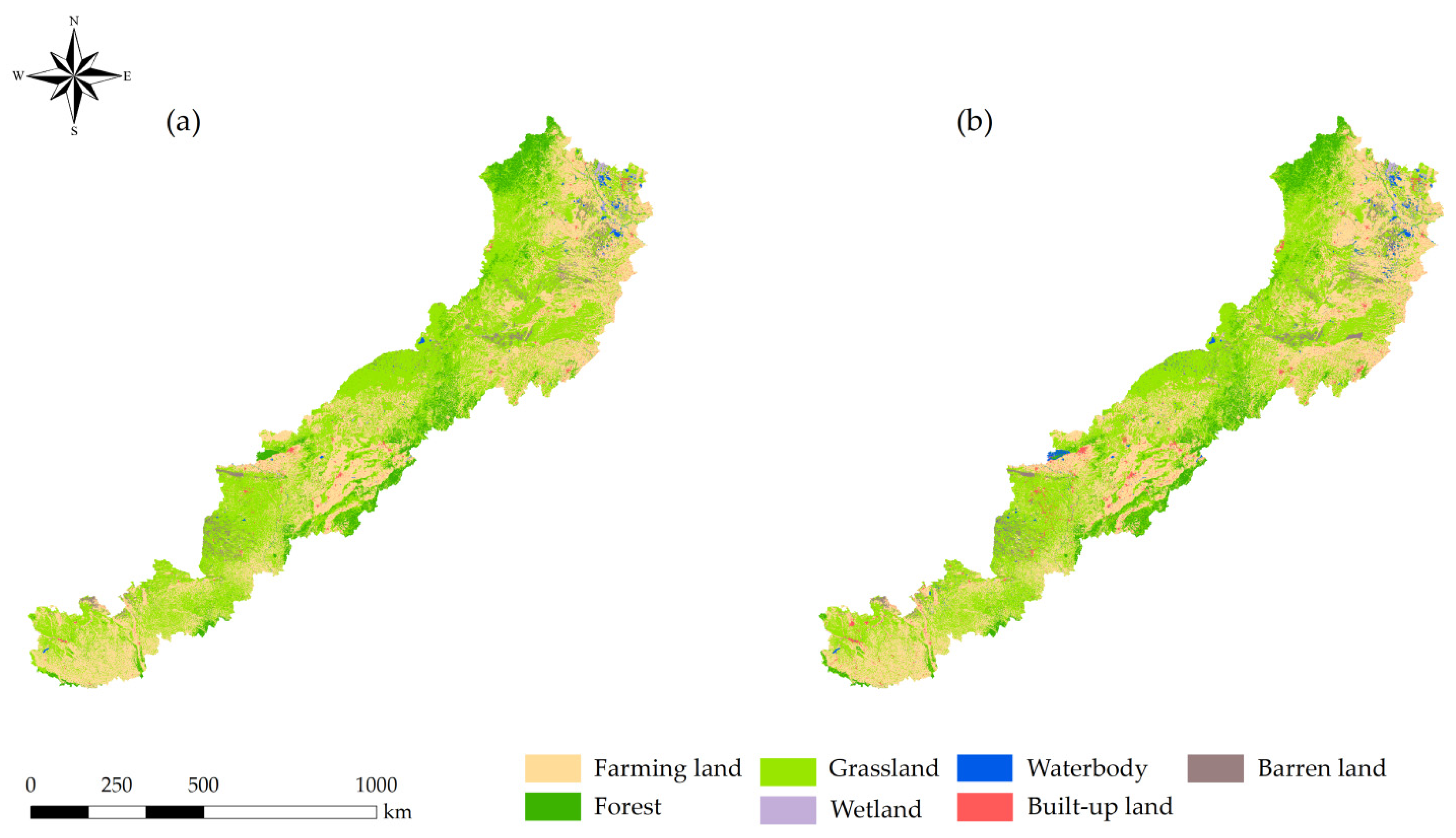
3.1. Land-Use Change (LUC)
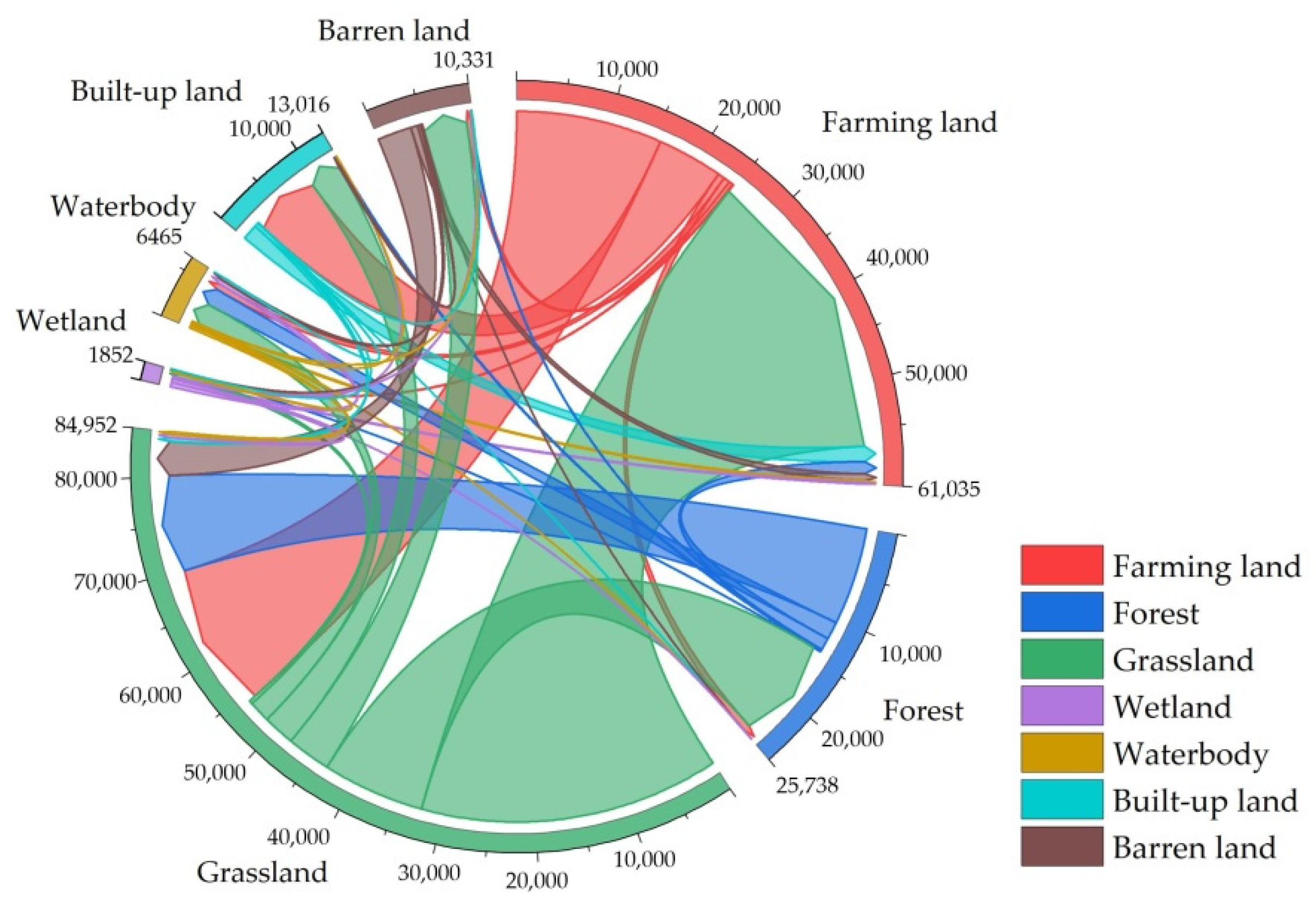
3.1.1. Land-Use Change (LUC) in the Past
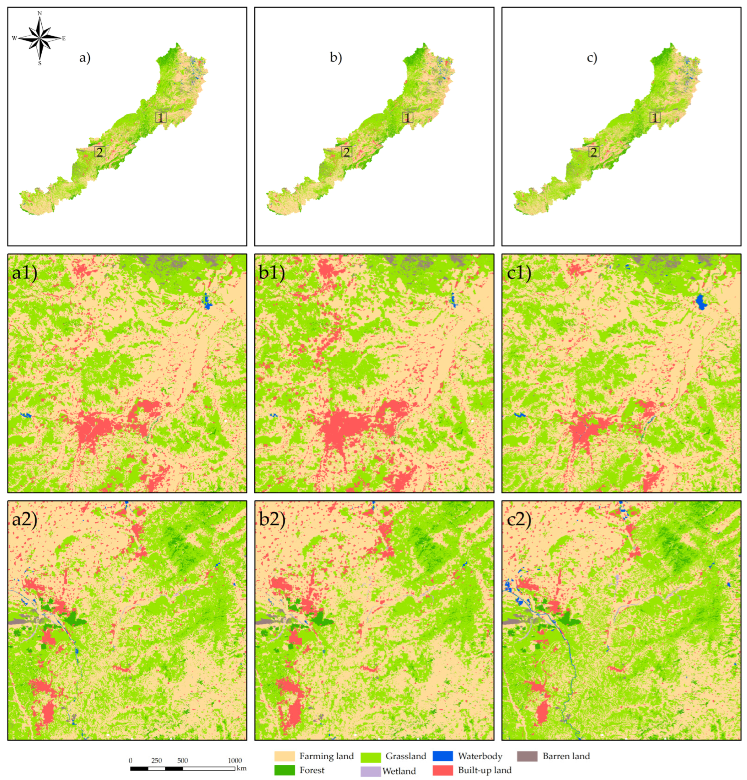
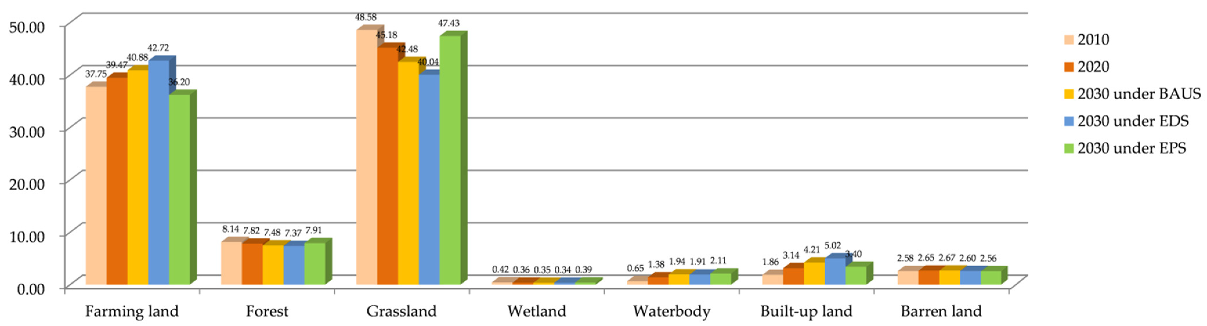
3.1.2. Land-Use Change (LUC) under the Scenarios
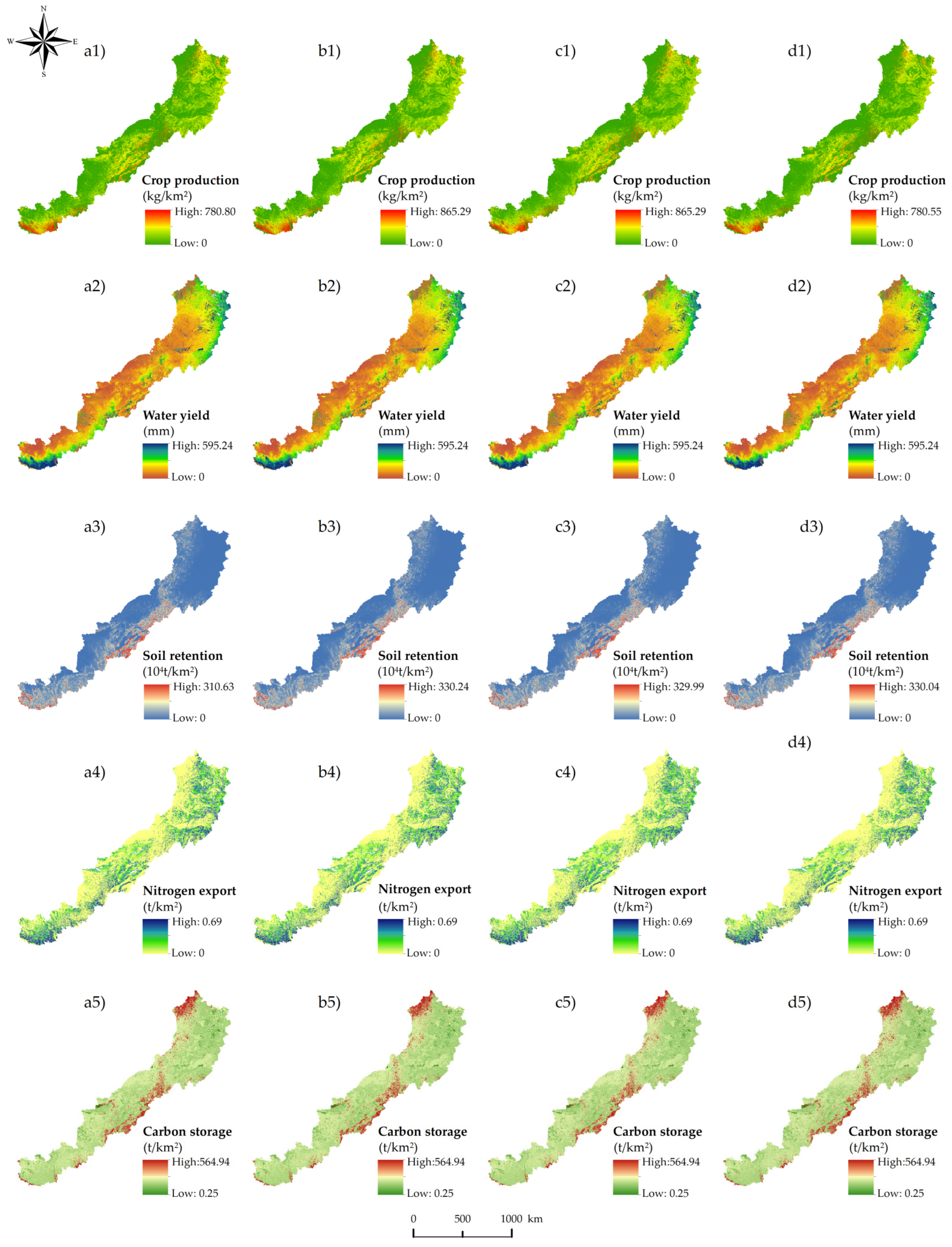
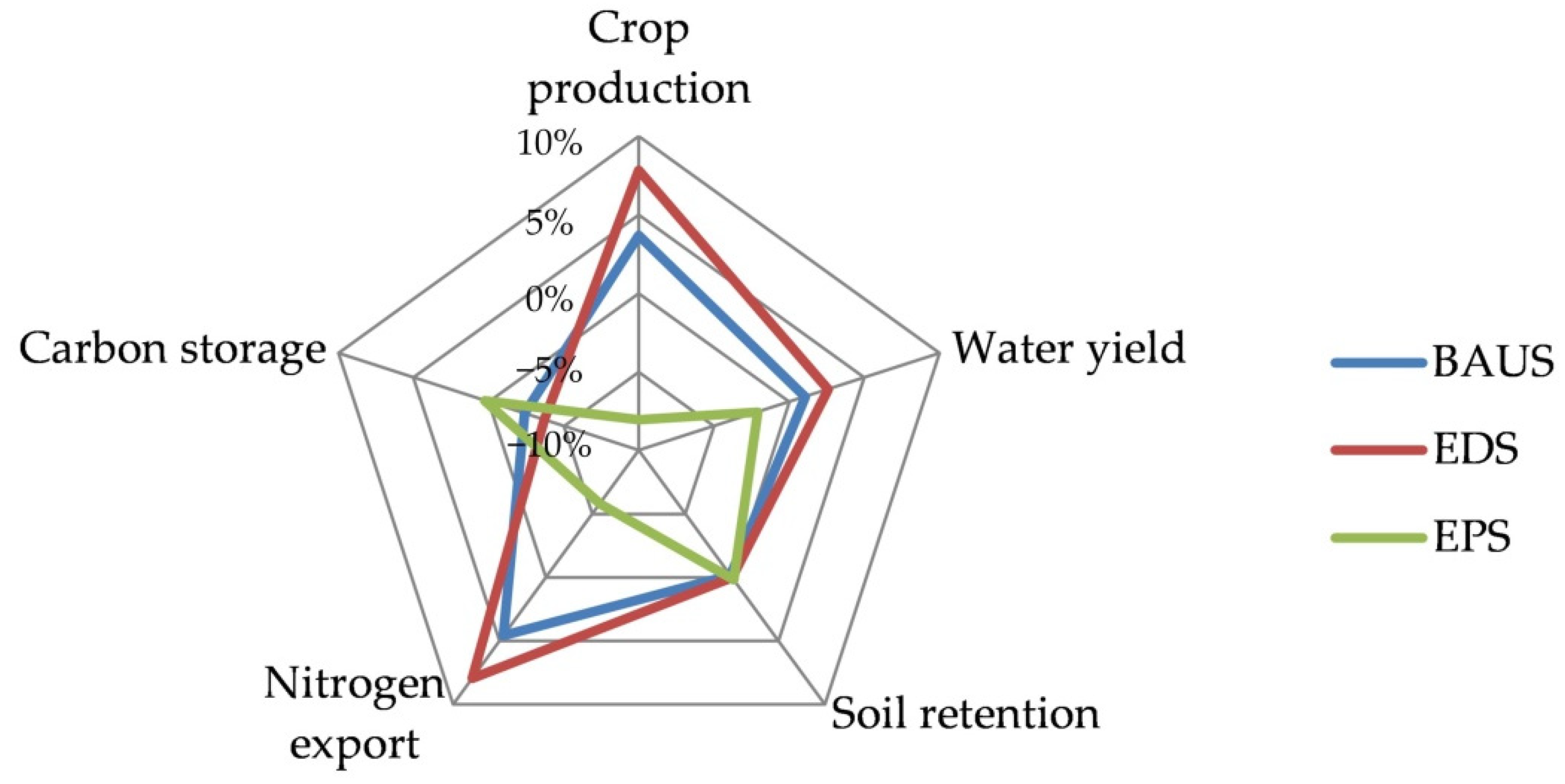
3.2. Comparison of the Ecosystem Services (ESs) under the Future Scenarios
3.3. Ecosystem Services (ESs) Trade-Offs
4. Discussion
4.1. Land-Use Change (LUC) and Its Impacts on Ecosystem Services (ESs) in the FPENC
4.2. Trade-Offs/Synergies under Different Scenarios
4.3. Suggestions for Future Regional Planning and Management
4.4. Limitations and Future Research
5. Conclusions
Author Contributions
Funding
Institutional Review Board Statement
Informed Consent Statement
Data Availability Statement
Conflicts of Interest
References
- Costanza, R.; d’Arge, R.; de Groot, R.; Farber, S.; Grasso, M.; Hannon, B.; Limburg, K.; Naeem, S.; O’Neill, R.V.; Paruelo, J.; et al. The Value of the World’s Ecosystem Services and Natural Capital. Nature 1997, 387, 253–260. [Google Scholar] [CrossRef]
- Millennium Ecosystem Assessment. Millennium Ecosystem Assessment Synthesis Report; Island Press: Washington, DC, USA, 2005. [Google Scholar]
- Brauman, K.A.; Daily, G.C.; Duarte, T.K.E.; Mooney, H.A. The Nature and Value of Ecosystem Services: An Overview Highlighting Hydrologic Services. Annu. Rev. Environ. Resour. 2007, 32, 67–98. [Google Scholar] [CrossRef]
- Mooney, H.; Larigauderie, A.; Cesario, M.; Elmquist, T.; Hoegh-Guldberg, O.; Lavorel, S.; Mace, G.M.; Palmer, M.; Scholes, R.; Yahara, T. Biodiversity, Climate Change, and Ecosystem Services. Curr. Opin. Environ. Sustain. 2009, 1, 46–54. [Google Scholar] [CrossRef]
- Bennett, E.M.; Peterson, G.D.; Gordon, L.J. Understanding Relationships among Multiple Ecosystem Services. Ecol. Lett. 2009, 12, 1394–1404. [Google Scholar] [CrossRef]
- Mitchell, M.G.E.; Suarez-Castro, A.F.; Martinez-Harms, M.; Maron, M.; McAlpine, C.; Gaston, K.J.; Johansen, K.; Rhodes, J.R. Reframing Landscape Fragmentation’s Effects on Ecosystem Services. Trends Ecol. Evol. 2015, 30, 190–198. [Google Scholar] [CrossRef] [PubMed] [Green Version]
- Dade, M.C.; Mitchell, M.G.E.; McAlpine, C.A.; Rhodes, J.R. Assessing Ecosystem Service Trade-Offs and Synergies: The Need for a More Mechanistic Approach. Ambio 2019, 48, 1116–1128. [Google Scholar] [CrossRef]
- Tomscha, S.A.; Gergel, S.E. Ecosystem Service Trade-Offs and Synergies Misunderstood without Landscape History. Ecol. Soc. 2016, 21, 43. [Google Scholar] [CrossRef] [Green Version]
- Bai, Y.; Ochuodho, T.O.; Yang, J. Impact of Land Use and Climate Change on Water-Related Ecosystem Services in Kentucky, USA. Ecol. Indic. 2019, 102, 51–64. [Google Scholar] [CrossRef]
- Costanza, R.; de Groot, R.; Sutton, P.; van der Ploeg, S.; Anderson, S.J.; Kubiszewski, I.; Farber, S.; Turner, R.K. Changes in the Global Value of Ecosystem Services. Glob. Environ. Chang. 2014, 26, 152–158. [Google Scholar] [CrossRef]
- Hasan, S.S.; Zhen, L.; Miah, M.G.; Ahamed, T.; Samie, A. Impact of Land Use Change on Ecosystem Services: A Review. Environ. Dev. 2020, 34, 100527. [Google Scholar] [CrossRef]
- Lang, Y.; Song, W. Quantifying and Mapping the Responses of Selected Ecosystem Services to Projected Land Use Changes. Ecol. Indic. 2019, 102, 186–198. [Google Scholar] [CrossRef]
- Kusi, K.K.; Khattabi, A.; Mhammdi, N.; Lahssini, S. Prospective Evaluation of the Impact of Land Use Change on Ecosystem Services in the Ourika Watershed, Morocco. Land Use Policy 2020, 97, 104796. [Google Scholar] [CrossRef]
- Zhang, Y.; Lu, X.; Liu, B.; Wu, D.; Fu, G.; Zhao, Y.; Sun, P. Spatial Relationships between Ecosystem Services and Socioecological Drivers across a Large-Scale Region: A Case Study in the Yellow River Basin. Sci. Total Environ. 2021, 766, 142480. [Google Scholar] [CrossRef] [PubMed]
- Clerici, N.; Cote-Navarro, F.; Escobedo, F.J.; Rubiano, K.; Villegas, J.C. Spatio-Temporal and Cumulative Effects of Land Use-Land Cover and Climate Change on Two Ecosystem Services in the Colombian Andes. Sci. Total Environ. 2019, 685, 1181–1192. [Google Scholar] [CrossRef]
- Pham, H.V.; Sperotto, A.; Torresan, S.; Acuña, V.; Jorda-Capdevila, D.; Rianna, G.; Marcomini, A.; Critto, A. Coupling Scenarios of Climate and Land-Use Change with Assessments of Potential Ecosystem Services at the River Basin Scale. Ecosyst. Serv. 2019, 40, 101045. [Google Scholar] [CrossRef]
- Arkema, K.K.; Verutes, G.M.; Wood, S.A.; Clarke-Samuels, C.; Rosado, S.; Canto, M.; Rosenthal, A.; Ruckelshaus, M.; Guannel, G.; Toft, J.; et al. Embedding Ecosystem Services in Coastal Planning Leads to Better Outcomes for People and Nature. Proc. Natl. Acad. Sci. USA 2015, 112, 7390–7395. [Google Scholar] [CrossRef] [Green Version]
- Gong, J.; Liu, D.; Zhang, J.; Xie, Y.; Cao, E.; Li, H. Tradeoffs/Synergies of Multiple Ecosystem Services Based on Land Use Simulation in a Mountain-Basin Area, Western China. Ecol. Indic. 2019, 99, 283–293. [Google Scholar] [CrossRef]
- Helfenstein, J.; Kienast, F. Ecosystem Service State and Trends at the Regional to National Level: A Rapid Assessment. Ecol. Indic. 2014, 36, 11–18. [Google Scholar] [CrossRef]
- Vlek, P.L.G.; Khamzina, A.; Azadi, H.; Bhaduri, A.; Bharati, L.; Braimoh, A.; Martius, C.; Sunderland, T.; Taheri, F. Trade-Offs in Multi-Purpose Land Use under Land Degradation. Sustainability 2017, 9, 2196. [Google Scholar] [CrossRef] [Green Version]
- Yang, S.; Zhao, W.; Liu, Y.; Wang, S.; Wang, J.; Zhai, R. Influence of Land Use Change on the Ecosystem Service Trade-Offs in the Ecological Restoration Area: Dynamics and Scenarios in the Yanhe Watershed, China. Sci. Total Environ. 2018, 644, 556–566. [Google Scholar] [CrossRef]
- Li, B.; Chen, D.; Wu, S.; Zhou, S.; Wang, T.; Chen, H. Spatio-Temporal Assessment of Urbanization Impacts on Ecosystem Services: Case Study of Nanjing City, China. Ecol. Indic. 2016, 71, 416–427. [Google Scholar] [CrossRef]
- Milnar, M.; Ramaswami, A. Impact of Urban Expansion and In Situ Greenery on Community-Wide Carbon Emissions: Method Development and Insights from 11 US Cities. Environ. Sci. Technol. 2020, 54, 16086–16096. [Google Scholar] [CrossRef] [PubMed]
- Ma, L.; Guo, J.; Velthof, G.L.; Li, Y.; Chen, Q.; Ma, W.; Oenema, O.; Zhang, F. Impacts of Urban Expansion on Nitrogen and Phosphorus Flows in the Food System of Beijing from 1978 to 2008. Glob. Environ. Chang. 2014, 28, 192–204. [Google Scholar] [CrossRef]
- Elias, E.; Dougherty, M.; Srivastava, P.; Laband, D. The Impact of Forest to Urban Land Conversion on Streamflow, Total Nitrogen, Total Phosphorus, and Total Organic Carbon Inputs to the Converse Reservoir, Southern Alabama, USA. Urban Ecosyst. 2013, 16, 79–107. [Google Scholar] [CrossRef]
- Chamberlain, D.; Kibuule, M.; Skeen, R.; Pomeroy, D. Trends in Bird Species Richness, Abundance and Biomass along a Tropical Urbanization Gradient. Urban Ecosyst. 2017, 20, 629–638. [Google Scholar] [CrossRef]
- Li, G.; Fang, C.; Li, Y.; Wang, Z.; Sun, S.; He, S.; Qi, W.; Bao, C.; Ma, H.; Fan, Y.; et al. Global Impacts of Future Urban Expansion on Terrestrial Vertebrate Diversity. Nat. Commun. 2022, 13, 1628. [Google Scholar] [CrossRef]
- Swetnam, R.D.; Fisher, B.; Mbilinyi, B.P.; Munishi, P.K.T.; Willcock, S.; Ricketts, T.; Mwakalila, S.; Balmford, A.; Burgess, N.D.; Marshall, A.R.; et al. Mapping Socio-Economic Scenarios of Land Cover Change: A GIS Method to Enable Ecosystem Service Modelling. J. Environ. Manag. 2011, 92, 563–574. [Google Scholar] [CrossRef]
- Teague, A.; Russell, M.; Harvey, J.; Dantin, D.; Nestlerode, J.; Alvarez, F. A Spatially-Explicit Technique for Evaluation of Alternative Scenarios in the Context of Ecosystem Goods and Services. Ecosyst. Serv. 2016, 20, 15–29. [Google Scholar] [CrossRef]
- Gao, J.; Li, F.; Gao, H.; Zhou, C.; Zhang, X. The Impact of Land-Use Change on Water-Related Ecosystem Services: A Study of the Guishui River Basin, Beijing, China. J. Clean. Prod. 2017, 163, S148–S155. [Google Scholar] [CrossRef]
- Ma, S.; Qiao, Y.P.; Jiang, J.; Wang, L.J.; Zhang, J.C. Incorporating the Implementation Intensity of Returning Farmland to Lakes into Policymaking and Ecosystem Management: A Case Study of the Jianghuai Ecological Economic Zone, China. J. Clean. Prod. 2021, 306, 127284. [Google Scholar] [CrossRef]
- Sharma, S.K.; Baral, H.; Laumonier, Y.; Okarda, B.; Purnomo, H.; Pacheco, P. Ecosystem Services under Future Oil Palm Expansion Scenarios in West Kalimantan, Indonesia. Ecosyst. Serv. 2019, 39, 100978. [Google Scholar] [CrossRef]
- Srichaichana, J.; Trisurat, Y.; Ongsomwang, S. Land Use and Land Cover Scenarios for Optimum Water Yield and Sediment Retention Ecosystem Services in Klong U-Tapao Watershed, Songkhla, Thailand. Sustainability 2019, 11, 2895. [Google Scholar] [CrossRef] [Green Version]
- Sun, S.; Shi, Q. Global Spatio-Temporal Assessment of Changes in Multiple Ecosystem Services under Four IPCC SRES Land-Use Scenarios. Earth’s Future 2020, 8, e2020EF001668. [Google Scholar] [CrossRef]
- Peng, J.; Hu, X.; Wang, X.; Meersmans, J.; Liu, Y.; Qiu, S. Simulating the Impact of Grain-for-Green Programme on Ecosystem Services Trade-Offs in Northwestern Yunnan, China. Ecosyst. Serv. 2019, 39, 100998. [Google Scholar] [CrossRef]
- Bai, Y.; Ouyang, Z.; Zheng, H.; Li, X.; Zhuang, C.; Jiang, B. Modeling Soil Conservation, Water Conservation and Their Tradeoffs: A Case Study in Beijing. J. Environ. Sci. 2012, 24, 419–426. [Google Scholar] [CrossRef]
- Wu, Y.; Tao, Y.; Yang, G.; Ou, W.; Pueppke, S.; Sun, X.; Chen, G.; Tao, Q. Impact of Land Use Change on Multiple Ecosystem Services in the Rapidly Urbanizing Kunshan City of China: Past Trajectories and Future Projections. Land Use Policy 2019, 85, 419–427. [Google Scholar] [CrossRef]
- Tian, Y.; Wang, S.; Bai, X.; Luo, G.; Xu, Y. Trade-Offs among Ecosystem Services in a Typical Karst Watershed, SW China. Sci. Total Environ. 2016, 566–567, 1297–1308. [Google Scholar] [CrossRef]
- Sun, X.; Zhang, Y.; Shen, Y.; Randhir, T.O.; Cao, M. Exploring Ecosystem Services and Scenario Simulation in the Headwaters of Qiantang River Watershed of China. Environ. Sci. Pollut. Res. 2019, 26, 34905–34923. [Google Scholar] [CrossRef]
- Li, Z.; Cheng, X.; Han, H. Analyzing Land-Use Change Scenarios for Ecosystem Services and Their Trade-Offs in the Ecological Conservation Area in Beijing, China. Int. J. Environ. Res. Public Health 2020, 17, 8632. [Google Scholar] [CrossRef]
- Shi, W.; Liu, Y.; Shi, X. Contributions of Climate Change to the Boundary Shifts in the Farming-Pastoral Ecotone in Northern China since 1970. Agric. Syst. 2018, 161, 16–27. [Google Scholar] [CrossRef]
- Chen, X.; Zhang, H.; Yao, X.; Zeng, W.; Wang, W. Latitudinal and Depth Patterns of Soil Microbial Biomass Carbon, Nitrogen, and Phosphorus in Grasslands of an Agro-Pastoral Ecotone. Land Degrad. Dev. 2021, 32, 3833–3846. [Google Scholar] [CrossRef]
- Yang, Y.; Wang, K.; Liu, D.; Zhao, X.; Fan, J. Effects of Land-Use Conversions on the Ecosystem Services in the Agro-Pastoral Ecotone of Northern China. J. Clean. Prod. 2020, 249, 119360. [Google Scholar] [CrossRef]
- Chen, C.; Huang, D.; Wang, K. Risk Assessment and Invasion Characteristics of Alien Plants in and Around the Agro-Pastoral Ecotone of Northern China. Hum. Ecol. Risk Assess. Int. J. 2015, 21, 1766–1781. [Google Scholar] [CrossRef]
- Wang, X.; Li, Y.; Chen, Y.; Lian, J.; Luo, Y.; Niu, Y.; Gong, X.; Yu, P. Temporal and Spatial Variation of Extreme Temperatures in an Agro-Pastoral Ecotone of Northern China from 1960 to 2016. Sci. Rep. 2018, 8, 8787. [Google Scholar] [CrossRef] [Green Version]
- Zhou, Z.; Sun, O.J.; Huang, J.; Li, L.; Liu, P.; Han, X. Soil Carbon and Nitrogen Stores and Storage Potential as Affected by Land-Use in an Agro-Pastoral Ecotone of Northern China. Biogeochemistry 2007, 82, 127–138. [Google Scholar] [CrossRef]
- Liu, J.; Chen, H.; Yang, X.; Gong, Y.; Zheng, X.; Fan, M.; Kuzyakov, Y. Annual Methane Uptake from Different Land Uses in an Agro-Pastoral Ecotone of Northern China. Agric. For. Meteorol. 2017, 236, 67–77. [Google Scholar] [CrossRef]
- Liu, M.; Jia, Y.; Zhao, J.; Shen, Y.; Pei, H.; Zhang, H.; Li, Y. Revegetation Projects Significantly Improved Ecosystem Service Values in the Agro-Pastoral Ecotone of Northern China in Recent 20 Years. Sci. Total Environ. 2021, 788, 147756. [Google Scholar] [CrossRef]
- Yang, Y.; Wang, K.; Liu, D.; Zhao, X.; Fan, J.; Li, J.; Zhai, X.; Zhang, C.; Zhan, R. Spatiotemporal Variation Characteristics of Ecosystem Service Losses in the Agro-Pastoral Ecotone of Northern China. Int. J. Environ. Res. Public Health 2019, 16, 1199. [Google Scholar] [CrossRef] [Green Version]
- Wang, Z.; Jiang, J.; Ma, Q. The Drought Risk of Maize in the Farming-Pastoral Ecotone in Northern China Based on Physical Vulnerability Assessment. Nat. Hazards Earth Syst. Sci. 2016, 16, 2697–2711. [Google Scholar] [CrossRef] [Green Version]
- Wang, Z.; Jiang, J.; Liao, Y.; Deng, L. Risk Assessment of Maize Drought Hazard in the Middle Region of Farming-Pastoral Ecotone in Northern China. Nat. Hazards 2015, 76, 1515–1534. [Google Scholar] [CrossRef]
- Xu, X. Spatial Distribution of GDP in China with Kilometer Grid Dataset. Resour. Environ. Sci. Data Regist. Publ. Syst. 2017. [Google Scholar] [CrossRef]
- Xu, X. Spatial Distribution of Chinese Population in Kilometer Grid Dataset. Resour. Environ. Sci. Data Regist. Publ. Syst. 2017. [Google Scholar] [CrossRef]
- Liu, X.; Liang, X.; Li, X.; Xu, X.; Ou, J.; Chen, Y.; Li, S.; Wang, S.; Pei, F. A Future Land Use Simulation Model (FLUS) for Simulating Multiple Land Use Scenarios by Coupling Human and Natural Effects. Landsc. Urban Plan. 2017, 168, 94–116. [Google Scholar] [CrossRef]
- Liao, W.; Liu, X.; Xu, X.; Chen, G.; Liang, X.; Zhang, H.; Li, X. Projections of Land Use Changes under the Plant Functional Type Classification in Different SSP-RCP Scenarios in China. Sci. Bull. 2020, 65, 1935–1947. [Google Scholar] [CrossRef]
- Li, X.; Chen, G.; Liu, X.; Liang, X.; Wang, S.; Chen, Y.; Pei, F.; Xu, X. A New Global Land-Use and Land-Cover Change Product at a 1-Km Resolution for 2010 to 2100 Based on Human–Environment Interactions. Ann. Am. Assoc. Geogr. 2017, 107, 1040–1059. [Google Scholar] [CrossRef]
- Li, J.; Chen, X.; Kurban, A.; Van de Voorde, T.; De Maeyer, P.; Zhang, C. Coupled SSPs-RCPs Scenarios to Project the Future Dynamic Variations of Water-Soil-Carbon-Biodiversity Services in Central Asia. Ecol. Indic. 2021, 129, 107936. [Google Scholar] [CrossRef]
- Liang, X.; Liu, X.; Li, X.; Chen, Y.; Tian, H.; Yao, Y. Delineating Multi-Scenario Urban Growth Boundaries with a CA-Based FLUS Model and Morphological Method. Landsc. Urban Plan. 2018, 177, 47–63. [Google Scholar] [CrossRef]
- Libang, M.; Shuwen, N.; Lina, Y. Scenarios Simulation of Land Use/Cover Pattern in Dunhuang City, Gansu Province of Northwest China Based on Markov and CLUE-S Integrated Model. Chin. J. Ecol. 2012, 31, 1823–1831. [Google Scholar]
- Fu, Q.; Hou, Y.; Wang, B.; Bi, X.; Li, B.; Zhang, X. Scenario Analysis of Ecosystem Service Changes and Interactions in a Mountain-Oasis-Desert System: A Case Study in Altay Prefecture, China. Sci. Rep. 2018, 8, 12939. [Google Scholar] [CrossRef]
- Chen, T.; Peng, L.; Wang, Q. Response and Multiscenario Simulation of Trade-Offs/Synergies among Ecosystem Services to the Grain to Green Program: A Case Study of the Chengdu-Chongqing Urban Agglomeration, China. Environ. Sci. Pollut. Res. 2022, 29, 33572–33586. [Google Scholar] [CrossRef]
- Cong, W.; Sun, X.; Guo, H.; Shan, R. Comparison of the SWAT and InVEST Models to Determine Hydrological Ecosystem Service Spatial Patterns, Priorities and Trade-Offs in a Complex Basin. Ecol. Indic. 2020, 112, 106089. [Google Scholar] [CrossRef]
- Sánchez-Canales, M.; López Benito, A.; Passuello, A.; Terrado, M.; Ziv, G.; Acuña, V.; Schuhmacher, M.; Elorza, F.J. Sensitivity Analysis of Ecosystem Service Valuation in a Mediterranean Watershed. Sci. Total Environ. 2012, 440, 140–153. [Google Scholar] [CrossRef] [PubMed]
- Guo, M.; Ma, S.; Wang, L.J.; Lin, C. Impacts of Future Climate Change and Different Management Scenarios on Water-Related Ecosystem Services: A Case Study in the Jianghuai Ecological Economic Zone, China. Ecol. Indic. 2021, 127, 107732. [Google Scholar] [CrossRef]
- Sharp, R.; Douglass, J.; Wolny, S.; Arkema, K.; Bernhardt, J.; Bierbower, W.; Chaumont, N.; Denu, D.; Fisher, D.; Glowinski, K.; et al. InVEST 3.11.0.post56+ug.gfa89dd9 User’s Guide; The Natural Capital Project, Stanford University, University of Minnesota, The Nature Conservancy, and World Wildlife Fund. 2020. Available online: https://invest-userguide.readthedocs.io/_/downloads/en/3.9.0/pdf/ (accessed on 17 March 2022).
- Erfu, D.; Xiaoli, W.; Jianjia, Z.; Dongsheng, Z. Methods, Tools and Research Framework of Ecosystem Service Trade-Offs. Geogr. Res. 2016, 35, 1005–1016. [Google Scholar]
- Luo, R.; Yang, S.; Wang, Z.; Zhang, T.; Gao, P. Impact and Trade off Analysis of Land Use Change on Spatial Pattern of Ecosystem Services in Chishui River Basin. Environ. Sci. Pollut. Res. 2022, 29, 20234–20248. [Google Scholar] [CrossRef] [PubMed]
- Yang, Y.; Li, M.; Feng, X.; Yan, H.; Su, M.; Wu, M. Spatiotemporal Variation of Essential Ecosystem Services and Their Trade-off/Synergy along with Rapid Urbanization in the Lower Pearl River Basin, China. Ecol. Indic. 2021, 133, 108439. [Google Scholar] [CrossRef]
- Zhou, J.; Zhang, F.; Xu, Y.; Gao, Y.; Xie, Z. Evaluation of Land Reclamation and Implications of Ecological Restoration for Agro-Pastoral Ecotone: Case Study of Horqin Left Back Banner in China. Chin. Geogr. Sci. 2017, 27, 772–783. [Google Scholar] [CrossRef]
- Tang, H.; Chen, Y.; Li, X. Driving Mechanisms of Desertification Process in the Horqin Sandy Land-a Case Study in Zhalute Banner, Inner Mongolia of China. Front. Environ. Sci. Eng. China 2008, 2, 487–493. [Google Scholar] [CrossRef]
- Ke, X.; Wang, L.; Ma, Y.; Pu, K.; Zhou, T.; Xiao, B.; Wang, J. Impacts of Strict Cropland Protection on Water Yield: A Case Study of Wuhan, China. Sustainability 2019, 11, 184. [Google Scholar] [CrossRef] [Green Version]
- Li, J.; Zhang, C.; Zhu, S. Relative Contributions of Climate and Land-Use Change to Ecosystem Services in Arid Inland Basins. J. Clean. Prod. 2021, 298, 126844. [Google Scholar] [CrossRef]
- Qiu, J.; Huang, T.; Yu, D. Evaluation and Optimization of Ecosystem Services under Different Land Use Scenarios in a Semiarid Landscape Mosaic. Ecol. Indic. 2022, 135, 108516. [Google Scholar] [CrossRef]
- Zhu, W.; Zhang, J.; Cui, Y.; Zhu, L. Ecosystem Carbon Storage under Different Scenarios of Land Use Change in Qihe Catchment, China. J. Geogr. Sci. 2020, 30, 1507–1522. [Google Scholar] [CrossRef]
- Procházková, E.; Kincl, D.; Kabelka, D.; Vopravil, J.; Nerušil, P.; Menšík, L.; Barták, V. The Impact of the Conservation Tillage “Maize into Grass Cover” on Reducing the Soil Loss Due to Erosion. Soil Water Res. 2020, 15, 158–165. [Google Scholar] [CrossRef]
- Vogel, E.; Deumlich, D.; Kaupenjohann, M. Bioenergy Maize and Soil Erosion-Risk Assessment and Erosion Control Concepts. Geoderma 2016, 261, 80–92. [Google Scholar] [CrossRef]
- Li, Q.; Zhang, X.; Liu, Q.; Liu, Y.; Ding, Y.; Zhang, Q. Impact of Land Use Intensity on Ecosystem Services: An Example from the Agro-Pastoral Ecotone of Central Inner Mongolia. Sustainability 2017, 9, 1030. [Google Scholar] [CrossRef] [Green Version]
- Yang, X.; Chen, H.; Gong, Y.; Zheng, X.; Fan, M.; Kuzyakov, Y. Nitrous Oxide Emissions from an Agro-Pastoral Ecotone of Northern China Depending on Land Uses. Agric. Ecosyst. Environ. 2015, 213, 241–251. [Google Scholar] [CrossRef]
- Liu, D.; Chen, J.; Ouyang, Z. Responses of Landscape Structure to the Ecological Restoration Programs in the Farming-Pastoral Ecotone of Northern China. Sci. Total Environ. 2020, 710, 136311. [Google Scholar] [CrossRef]
- Chen, J.; John, R.; Sun, G.; Fan, P.; Henebry, G.M.; Fernández-Giménez, M.E.; Zhang, Y.; Park, H.; Tian, L.; Groisman, P.; et al. Prospects for the Sustainability of Social-Ecological Systems (SES) on the Mongolian Plateau: Five Critical Issues. Environ. Res. Lett. 2018, 13, 123004. [Google Scholar] [CrossRef]
- Wang, Q.; Guan, Q.; Lin, J.; Luo, H.; Tan, Z.; Ma, Y. Simulating Land Use/Land Cover Change in an Arid Region with the Coupling Models. Ecol. Indic. 2021, 122, 107231. [Google Scholar] [CrossRef]
- Tan, Z.; Guan, Q.; Lin, J.; Yang, L.; Luo, H.; Ma, Y.; Tian, J.; Wang, Q.; Wang, N. The Response and Simulation of Ecosystem Services Value to Land Use/Land Cover in an Oasis, Northwest China. Ecol. Indic. 2020, 118, 106711. [Google Scholar] [CrossRef]
- Hu, S.; Chen, L.; Li, L.; Zhang, T.; Yuan, L.; Cheng, L.; Wang, J.; Wen, M. Simulation of Land Use Change and Ecosystem Service Value Dynamics under Ecological Constraints in Anhui Province, China. Int. J. Environ. Res. Public Health 2020, 17, 4228. [Google Scholar] [CrossRef] [PubMed]
- Li, M.; Liu, S.; Wang, F.; Liu, H.; Liu, Y.; Wang, Q. Cost-Benefit Analysis of Ecological Restoration Based on Land Use Scenario Simulation and Ecosystem Service on the Qinghai-Tibet Plateau. Glob. Ecol. Conserv. 2022, 34, e02006. [Google Scholar] [CrossRef]
- Ghimire, U.; Shrestha, S.; Neupane, S.; Mohanasundaram, S.; Lorphensri, O. Climate and Land-Use Change Impacts on Spatiotemporal Variations in Groundwater Recharge: A Case Study of the Bangkok Area, Thailand. Sci. Total Environ. 2021, 792, 148370. [Google Scholar] [CrossRef] [PubMed]


| Formulas | Description | References | |
|---|---|---|---|
| CP | refers to the crop production in pixel x(t), refers to the total crop yield (t), refers to the NPP of grid i, and refers to the sum of the regional NPP. | [61] | |
| WY | refers to water yield for the landscape x, refers to the actual evapotranspiration for pixel x, and refers to the actual precipitation on pixel x. | [65] | |
| SR | USLE is the amount of soil loss; R is rainfall erosivity; K is soil erodibility; LS is a slope length–gradient factor; C is vegetation cover management factor; P is support practice factor; SR is the amount of soil retention. | [65] | |
| NE | refers to the nitrogen export on pixel i, refers to the modified nitrogen load on pixel i, and refers to nitrogen delivery ratio on pixel i. | [65] | |
| CS | refer to total carbon, aboveground biomass, belowground biomass, soil organic carbon, and dead matter, respectively. | [65] |
| Crop Production (104 ton) | Water Yield (108 m3) | Soil Retention (108 ton) | Nitrogen Export (104 kg) | Carbon Storage (108 ton) | |
|---|---|---|---|---|---|
| 2020 | 6628.24 | 322.02 | 16.71 | 7112.37 | 21.65 |
| BAUS | 6872.81 | 325.39 | 16.68 | 7437.50 | 21.13 |
| EDS | 7148.08 | 330.49 | 16.60 | 7704.70 | 20.87 |
| EPS | 6095.66 | 315.15 | 16.74 | 6665.30 | 21.70 |
Publisher’s Note: MDPI stays neutral with regard to jurisdictional claims in published maps and institutional affiliations. |
© 2022 by the authors. Licensee MDPI, Basel, Switzerland. This article is an open access article distributed under the terms and conditions of the Creative Commons Attribution (CC BY) license (https://creativecommons.org/licenses/by/4.0/).
Share and Cite
Bai, S.; Yang, J.; Zhang, Y.; Yan, F.; Yu, L.; Zhang, S. Evaluating Ecosystem Services and Trade-Offs Based on Land-Use Simulation: A Case Study in the Farming–Pastoral Ecotone of Northern China. Land 2022, 11, 1115. https://doi.org/10.3390/land11071115
Bai S, Yang J, Zhang Y, Yan F, Yu L, Zhang S. Evaluating Ecosystem Services and Trade-Offs Based on Land-Use Simulation: A Case Study in the Farming–Pastoral Ecotone of Northern China. Land. 2022; 11(7):1115. https://doi.org/10.3390/land11071115
Chicago/Turabian StyleBai, Shuting, Jiuchun Yang, Yubo Zhang, Fengqin Yan, Lingxue Yu, and Shuwen Zhang. 2022. "Evaluating Ecosystem Services and Trade-Offs Based on Land-Use Simulation: A Case Study in the Farming–Pastoral Ecotone of Northern China" Land 11, no. 7: 1115. https://doi.org/10.3390/land11071115
APA StyleBai, S., Yang, J., Zhang, Y., Yan, F., Yu, L., & Zhang, S. (2022). Evaluating Ecosystem Services and Trade-Offs Based on Land-Use Simulation: A Case Study in the Farming–Pastoral Ecotone of Northern China. Land, 11(7), 1115. https://doi.org/10.3390/land11071115