Article

Assessment of the Relationship between Land Use and Flood Risk Based on a Coupled Hydrological–Hydraulic Model: A Case Study of Zhaojue River Basin in Southwestern China

Key Laboratory of Earth Surface Processes of Ministry of Education, College of Urban and Environmental Sciences, Peking University, Beijing 100871, China
*
Author to whom correspondence should be addressed.
Land 2022, 11(8), 1182; https://doi.org/10.3390/land11081182
Submission received: 23 June 2022 / Revised: 26 July 2022 / Accepted: 26 July 2022 / Published: 28 July 2022
(This article belongs to the Special Issue Ecosystem-Based Regional Planning)

Abstract

:
As an ecological consequence of intensified anthropogenic activities, more frequent extreme rainfalls have resulted in significant increases in water levels and discharge in southwestern China. This phenomenon presents a significant challenge in flood risk and ecological management. Land use is one of the major factors significantly affecting the flooding process, and it is inextricably tied to the ecological risk of floods. Hence, flood risk estimates based on land use are essential for flood control and land use planning. In this study, a coupled hydrologic–hydraulic model was developed to analyze the relationship between flood ecological risk and land use in order to provide new insights into current flood risk management practices. Ten real flood events (of different magnitudes) in the Zhaojue river basin (650 km2) were chosen to evaluate the credibility and performance of the coupled model’s application. Promising results were obtained, with sufficient reliability for flood risk assessment purposes. The results of our flood risk analysis also indicated that the model effectively reproduced overland flow and competently accounted for flood evolution. This work is significant in the understanding of the mechanism of the flood process and its relationship with land use, and it can be used in decision support for the prevention and mitigation of flood disasters and for land use planning.

1. Introduction

Floods are considered the most common and damaging natural hazards around the world [1,2,3,4], in which they cause over 50% of all casualties and more than 30% of economic losses [5]. The frequency of extreme rainfall events has grown with increases in population and the acceleration of urbanization, and the damage caused by floods has gradually become one of the biggest risks to social development worldwide [6,7,8]. At present, the frequency, intensity, loss, and ranges of impacts of flood disasters in the world have shown significant upward trends [9,10], demonstrating that flood control and disaster mitigation still face challenges. China has some of the most severe flood disasters in the world [11,12,13,14]. Floods have become a comprehensive problem that cannot be disregarded in sustainable development, which has increased pressure on local water resource management departments in flood management and prevention.
Flood risk reduction requires flood risk assessment [15,16,17], which is an essential component of flood control and disaster mitigation and plays an important role in flood management as a non-engineering measure [18]. With the rapid development of 3S technology, numerical calculation techniques, and flood simulation technology, flood risk assessment has received more and more attention in flood control and emergency work [18]. Studies have demonstrated that reasonable flood risk assessment can provide crucial information (such as inundation extent, water depth, flow velocity, peak flow, and arrival time) for strategy development and planning adaptation [19]. Attems et al. emphasized that flood risk assessment should be applied to flood management as a non-structural measure alongside structural measures [20]. Costache et al. suggested that flood risk assessment is an essential and mandatory procedure that should be included in flood management strategies [21]. Wu et al. proposed a hydrodynamic model for flood risk assessment in different environments that could be used to provide support for urban flood control and flood risk management [22]. Lowe et al. combined multiple models to systematically test various flood risks [23]. Mehr et al. used a forecasting system for flood risk assessment and achieved good results [24]. Furthermore, numerous large-scale flood risk map projects have been established by national institutions, thus attaching serious importance to flood risk assessment [25].
Previous studies have shown that land use associated with anthropogenic activities is the main factor affecting runoff and flooding [26,27,28,29,30], causing more flood risks [31,32,33]. Related research has suggested that land use change is the strongest contributor to changes in the flood process that may be directly responsible for more than 70% of floods worldwide [34,35]. Various land use types, such as urbanization [36], cultivated land [37], and vegetation changes [38,39], have disparate hydrological consequences. Land use structures and patterns also play important roles in the flood process [40,41]. Overall, land use planning has a potentially significant effect on flood risk. Ran et al. pointed out that flood risk management should be integrated and investigated in tandem with land use planning [42]. According to related research [43], reasonable land use planning based on flood risk analysis could decrease future flood risks by 39–50%, so increased flood risks caused by unreasonable land use also require attention [44]. Hence, flood risk assessment guided by the land–flood dual ecosystem theory needs to be studied [45].
Flood risk assessment in southwestern China has become more urgent due to its complex and unique characteristics [46,47,48,49]. For instance, 10% of China’s area comprises hills and mountains, with slopes of greater than 15° accounting for 60.0% of the terrain, demonstrating that this region is at serious flood risk [50]. Hence, compared to other regions, the flood control and disaster mitigation of China may face greater challenges.
As the core contents of flood risk assessment, coupled hydrological–hydraulic models have been increasingly appreciated in recent decades [51,52,53,54]. Coupled models can consider the effects of land use on the flooding process, so these models have been widely applied as important tools for flood management and land use planning [55,56,57,58,59,60]. On the one hand, hydrological models have major advantages over current alternatives in terms of modeling complex situations, computational efficiency, and imputation accuracy. On the other hand, hydraulic models have the ability to characterize hydrological behavior information in detail, laying the foundation for refined flood risk analysis [61]. Hence, hydrological–hydraulic coupled models can be used when a single model cannot meet simulation requirements. By linking hydrology to hydrodynamics, it is possible to increase the advantages and compensate for the weaknesses of both [57]. Flood behavior can be described more accurately from the different perspectives with their respective advantages. Lai et al. presented a coupled numerical model and successfully reproduced the flow regime of the Yangtze river basin [62]. Paiva et al. coupled an MGB–IPH hydrological model and a hydrodynamic model to simulate the flood process in the Amazon basin, and their results showed that the coupled model could reproduce the main hydrological characteristics [63]. Yin et al. applied coupled models to predict the flow and inundation of rivers and obtained information on the spatial distribution of floods [64]. Lian et al. employed a hydrology–hydrodynamic coupling model to simulate the flow of the Illinois river basin at different time scales, and the results showed that the accuracy of the coupled model was higher than that of a single model [65]. The same conclusion was drawn in a related paper [66].
Though there have been numerous studies based on coupled models for flood events, combining the advantages of both on the basin scale still faces many problems [67,68] regarding, e.g., the space–time scale [54,55,69], numerical instabilities [57,70], realistic flood events [71], validation issues [68,72], regional parameterization [54,73], infiltration issues [74], stream flow allocation issues [75], and connectivity issues [76,77]. To date, fully coupled modeling studies in realistic basins with both rainfall and infiltration processes have been rare, and coupling lumped rainfall–runoff (RR) models and fully dynamic hydraulic models have not been frequently reported in the literature [77].
Therefore, to fill the current research and practical gaps, our work aimed to develop a flood risk assessment approach using an integrated lumped RR and two-dimensional hydraulic model (2D) in realistic flood events incorporating both rainfall and infiltration processes. Land use information was adopted to solve the regional parameterization of the basin. The Zhaojue river basin in southwestern China was selected as a case study to assess the model’s performance. We also investigated the relationship between land use and flood risk in the basin. The proposed analytical method and knowledge gained from this study could help land use decision-makers and planners to identify flooded risk areas prior to future land use development. The remainder of this paper is organized as follows: Section 2 describes the methods and study area, Section 3 summarizes the research results, discussions are provided in Section 4, and conclusions are drawn in Section 5.

2. Materials and Methods

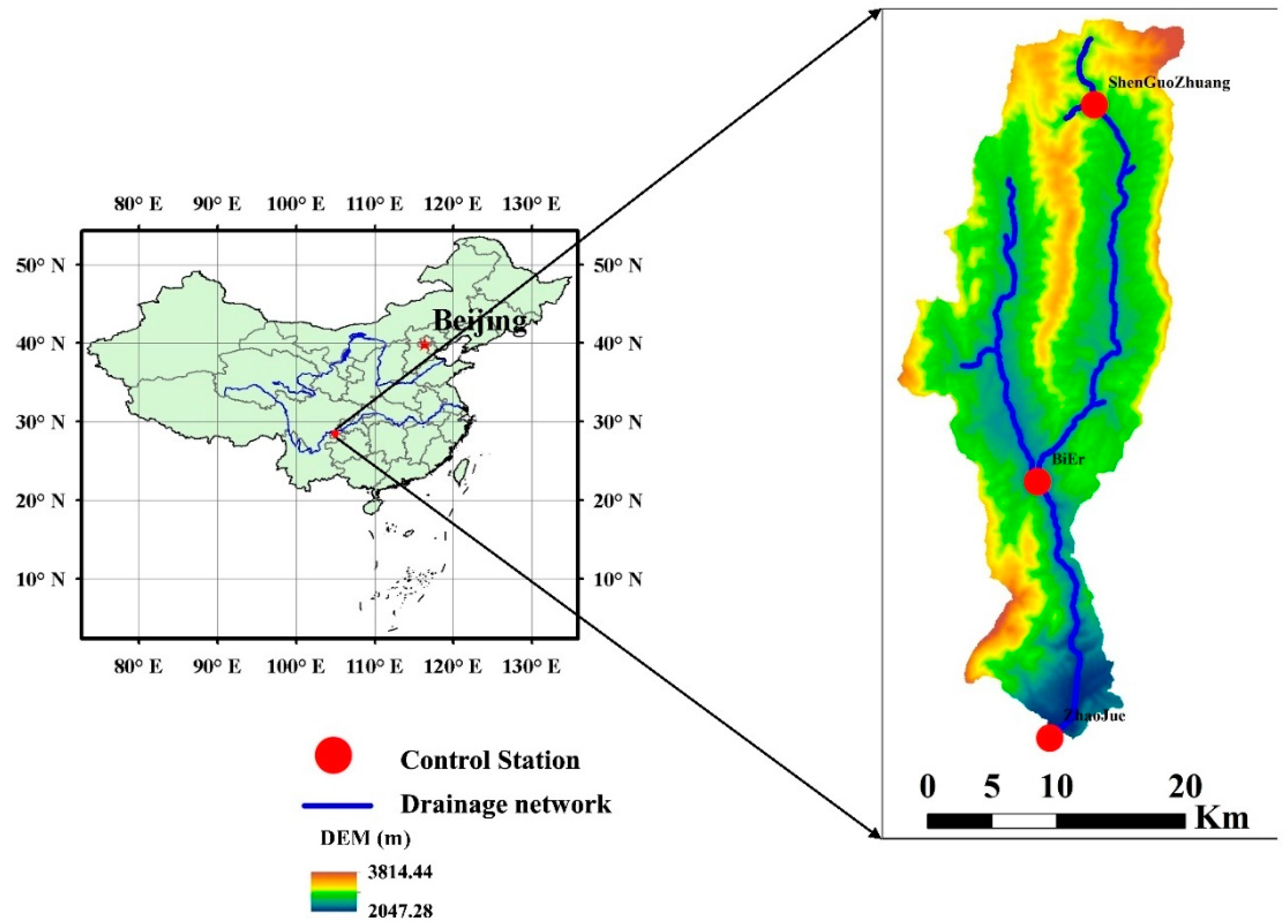
2.1. Study Area and Data Description

The study was conducted in a typical southwestern mountainous basin: the Zhaojue river basin with different hillslopes, soil properties, and vegetative covers. The Zhaojue river basin is located in Liangshan Yi Autonomous Prefecture, in the southwest of Sichuan province, China, with an area of 650 km2 (28.00°–28.51° N, 102.69°–102.91° E) (Figure 1). It is a second-order tributary of the Jinsha River. There are three rainfall stations and a hydrologic station in this basin: ShenGuoZhuang station, SuoLuo station, Bier station, and Zhaojue hydrologic station. Elevation in the basin ranges from 2047 to 3815 m, and its surface relief and slope are significantly steep. These topographies are more likely to trigger extreme rainfall and flooding events, resulting in considerable infrastructure damage and losses of life.
Extreme rainfall events frequently occur in this region due to climate change and the influence of the southwest monsoon [78,79]. Additionally, due to its complex terrain and geological, ecological, and social backgrounds, rainfall events can easily cause flooding and threaten the safety of people’s lives and property [80,81] (Figure 2). Furthermore, related research suggests that there will be considerably more flooding in this area in the future [82]. Hence, the flood risk analysis of this area is of practical importance.
The dataset used in this study included rainfall, evaporation, discharge, DEM, and land use information. Details of the various data types used in this study are given in Table 1.

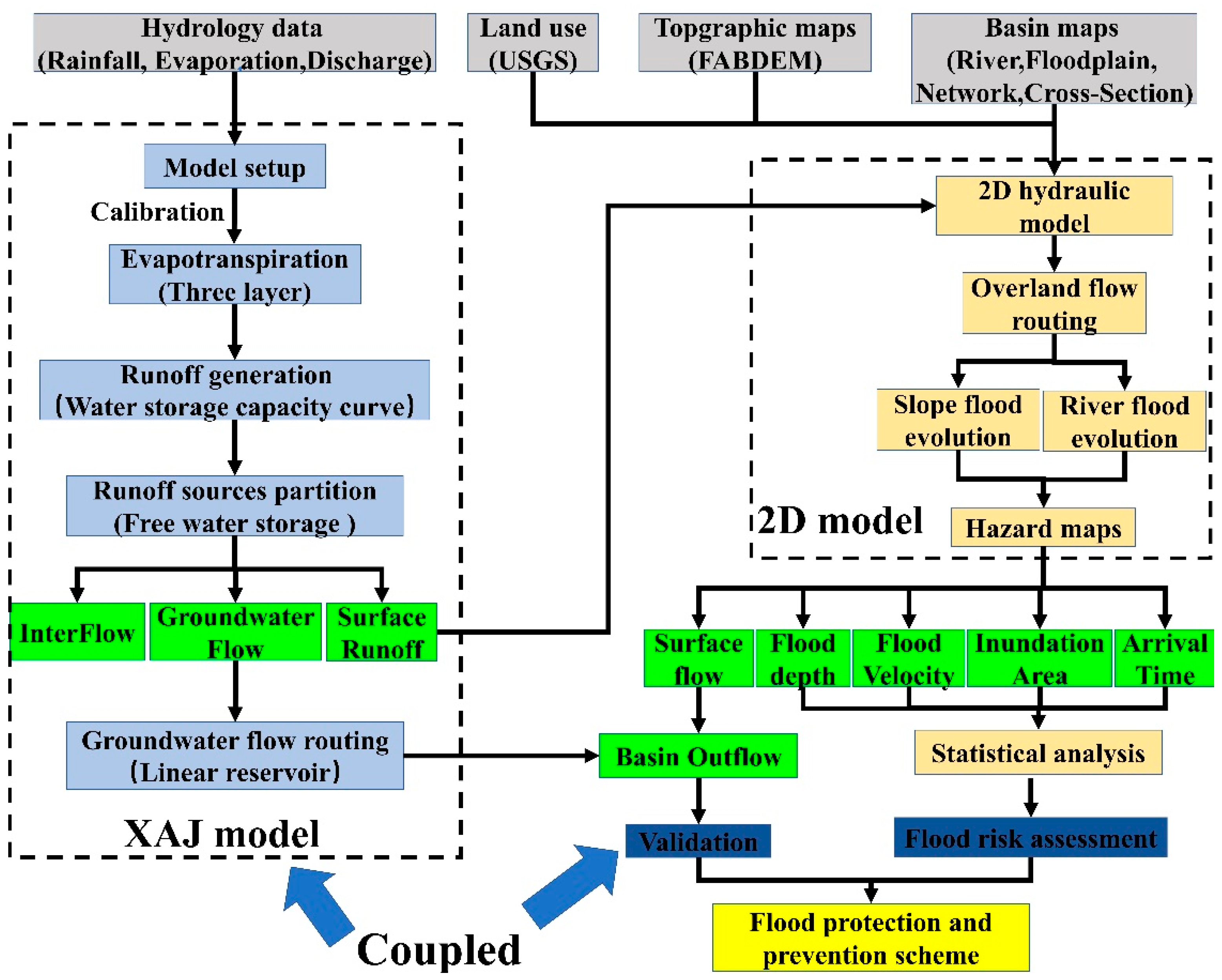
2.2. Description of the Coupled Model

The coupled model was constructed based on a lumped hydrological model (XAJ) and a hydraulic model (2D model). In the coupling framework, the XAJ model was adopted to generate runoff, and the routing scheme was replaced by the 2D model (discretized surface runoff as input) to better simulate flash floods at the basin scale. The whole coupling process is illustrated in Figure 3.
With hourly rainfall, evaporation, and discharge data, the XAJ model served as a rainfall–runoff generator that generates surface runoff, interflow and groundwater flow after evapotranspiration, runoff generation, and runoff source partition (including a priori calibration) data (Figure 3, left). After these processes, the routing processes of interflow and groundwater flow still used the XAJ model (linear reservoir method). However, the routing technique of surface runoff was replaced by the 2D model to analyze flood evolution. The discretized surface flow was moved from upstream to downstream over the entire basin through a topography-based cell-to-cell connectivity sequence. Additionally, the Manning coefficient (derived from land use) was used to estimate the flow resistance to adjust the effect of underlying surface on water flow velocity (Figure 3, upper right). The model was verified by comparing the sum of the discharge at the basin outlet from the 2D model and the underground discharge from the XAJ model with the measured discharge. Additionally, more flash flood information (flood depth, velocity, inundation area, and arrival time) could be obtained by the coupled model. The analysis of this information could contribute to reducing flood hazards and associated consequences (Figure 3, lower right). The remainder of this section details the components of the coupled model.

2.2.1. Hydrologic Component (XAJ)

The XAJ model was developed by Zhao et al. [83]; it is one of the most famous lumped hydrological models based on saturation excess runoff and is widely used in the humid and semi-humid basins of China [84]. The XAJ model uses four main components: evapotranspiration, runoff generation, runoff source partition, and runoff routing (Figure 4). Here, the three-layer evapotranspiration sub-model was utilized to calculate the evaporation, and a tension water storage capacity curve was adopted to generate the total runoff.
Runoff generation is one of the most important modules of the model, and a parabolic curve was used to calculate the runoff yield, which could be approximately represented by the following equation:
f F = 1   -   ( 1   -   W m W m m ) B ,
{ R = P E W M + W 0 + W M [ 1 ( P E + A ) / W m m ] 1 + B P E + A < W m m R = P E W M + W 0 P E + A W m m ,
where W m is the tension water storage capacity of a point in the basin (mm), f is the fraction of the basin area for which the storage capacity is less than W m , F is the whole basin area, W m m is the maximum value of W m , B is the shape parameter of the storage capacity distribution, R is the total runoff, P is the rainfall, E is the evapotranspiration, WM is the average tension water storage capacity, W 0 is the initial soil water storage, and A is the initial state of the basin.
The total runoff is composed of surface runoff, interflow, and groundwater runoff by a free water capacity curve:
FS F R = 1   -   ( 1   -   S M F SMMF ) EX ,
where S M F is the free water storage capacity of a point in the basin, SMMF is the maximum value of S M F , FS is the fraction of the basin area for which the free water storage is less than S M F , FR is the runoff-producing area proportion, and EX is the exponent of the free water storage capacity curve.
The surface runoff was set to be routed with the unit hydrograph or the lag-and-route method. The interflow and groundwater flow were set to be routed with the linear reservoir method [85]. The outflow of each sub-basin was set to be routed to the basin outlet with the Muskingum method [86].

2.2.2. Hydraulic Component (2D Model)

The two-dimensional hydraulic model was used to solve the 2D shallow water equations (SWEs) based on the principles of the conservation of mass and the conservation of momentum under steady-state flow conditions [61,87,88]. The method was developed for simulating two-dimensional overland flow with spatially variable infiltration and microtopography using hydrodynamic flow equations [89].
In order to ensure well-balanced properties when the grids near the dry and wet interface in the calculation domain are processed separately, water depth is treated as the water level in this model [88]. The two-dimensional hydraulic model can be represented as follows:
q t + f x + g y = s ,
where q is the vector containing the conserved flow variables, x and y are the Cartesian directions, f and g are the flux vector terms in the two Cartesian directions, t is time, and s is a source term.
Furthermore,
q = [ η h u h v ] ,   f = [ h u u 2 h + 1 2 u v h g ( η 2 2 η z b ) ] ,     g = [ h v h v u h v 2 + 1 2 g ( η 2 2 η z b ) ] ,
s = [ 0 τ b x ρ g h z b x τ b y ρ g h z b y ] ,
where η is the water surface elevation, h is the total water depth, u and v are the two Cartesian velocity components,   g is the acceleration due to gravity,   z b is the bed elevation above datum,   ρ is the water density, and τ b x and τ b y are the friction stresses that can be represented as follows:
τ b x = ρ C f u u 2 + v 2 , τ b y = ρ C f v u 2 + v 2 ,
C f = g n 2 h 1 3 ,
where C f is the roughness coefficient and n is the Manning coefficient.

2.2.3. Coupled Component (Coupled Model)

The 2D hydraulic model described in Section 2.2.2 only deals with movement in the horizontal direction, even though water flows vertically in addition to horizontally between soils in the entire process of the water cycle. The model additionally lacks the ability to convert rainfall into surface runoff (it cannot handle the infiltration process). Hence, we had to integrate the surface runoff generated from Equation (3) into Equation (6) to build the coupled model. Hence, in the coupled model, the s variable in Equation (6) needed to be adjusted to the following:
s = [ R s u r τ b x ρ g h z b x τ b y ρ g h z b y ] ,
where R s u r is the surface runoff. Ultimately, by integrating Equation (9) into Equation (4), the coupled model could be constructed. In the coupled model, the infiltration component is represented by the XAJ model, and the routing scheme of the XAJ model is replaced by the two-dimensional (2D) hydraulic model.
The R s u r obtained by the XAJ model is only the mean value of the basin, so a certain theory was needed to assign R s u r to each grid in the basin to obtain the discretized surface runoff. The spatially discretized surface runoff based on land use can be represented as follows:
R s u r ,   i = f ( p e , s , l , r , S M , E X ) ,
where R s u r , i is the surface runoff of the i-th grid;   p is the rainfall;   e is the evaporation;   s is the soil water content of free water;   l is the land use;   r is the contributing area of runoff;   S M is the free water capacity;   E X is the parameter of the free water capacity curve;   p and e are observed values;   s ,   r ,   S M ,   and   E X can be obtained by the XAJ model; and l can be obtained from the land use information. Overall, by integrating Equations (9) and (10) into Equation (4), the coupled model could be constructed.

2.3. Data Preprocessing and Model Calibration

According to the requirements of Equations (1) to (10), the main data preprocessing steps were established with the aid of GIS tools and remote sensing data. We used a digital elevation model (DEM) as the main input for topographic parameter extraction in both hydrological and hydraulic modeling for the preprocessing of data regarding, e.g., sub-basins, drainage networks, slope, directions of water flow, and cross-sectional profiles. FABDEM was adopted to identify and extract these features. The average areal rainfall in each sub-basin was calculated with the Thiessen polygonal method [90]. Manning’s coefficient was determined according to land use to reflect the surface roughness in this study (Table 2), and such values were supported by a number of previous works [61,91].
The model calibration aimed to align the model’s results with observed data by adjusting the model parameters, which was crucial for model application. The PEST (Parameter Estimation) automatic calibration algorithm is a flexible and generic calibration tool that can be used in any of these models and has been widely applied [92]. Hence, the PEST algorithm was linked to the coupled model in the MATLAB environment for model calibration and validation in our study. The calibration procedure was used to optimize 13 parameters (Table 3) related to evapotranspiration (K, C, WUM, WLM, and WDM), runoff generation (B and IMP), runoff source partition (SM and EX), and runoff routing (KI, KG, KKI, and KKG) following the work of Zhao et al. [83]. Three main factors were considered during parameter optimization: the upper and lower bounds of each parameter, the objective function, and the iteration termination criteria. The upper and lower bounds were determined by the model’s recommended parameter range and their physical meaning to avoid the selection of localized parameter values (Table 3) [83,93,94]. The objective function was calculated as follows:
F = i = 1 n ( Q s Q o ) 2 ,
where F is an objective function, Q s is the simulated discharge, and Q o is the observed discharge.
Ten significant flood events in the period of 2005–2010 were available for the study. We used six flood events to calibrate the model, and the others were used for validation purposes (the results are introduced in Section 3.2).
A uniform grid spacing of 30 m was used, so the entire basin had more than 700,000 grid points. At each grid point, hydraulic conductivity based on the remote sensing data was defined. According to the definition of a drainage watershed, all surface water located within the watershed ultimately converged to an outlet. Therefore, the coupled model only needed two types of “known” boundary conditions, i.e., non-transmissible (wall) for all boundaries except for an outlet and transmissible (open) boundary conditions for outlets. A time interval of 1 s was used for the simulation. The simulations were carried out in a continuous fashion and included the representation of subsurface and surface dynamics, and the output time interval was 1 h. The time step used for hydraulic routing was 0.5 s, which could be adaptively increased according to the local CFL conditions.

2.4. Statistical Method

The performance of the coupled model could be computed using statistical indices and graphical comparisons. The Nash–Sutcliffe efficiency (NSE), relative error (RE), peak discharge error (PE), and time difference of arrival peak discharge ( Δ T ) were employed to estimate the model’s performance [96].
NSE = 1   -     ( Q o - Q s ) 2   ( Q o - Q o ¯ ) 2 ,
RE =   Q s -   Q o   Q o   ×   100 % ,
PE = MAX ( Q s ) - MAX ( Q o ) MAX ( Q o )   ×   100 % ,
Δ T = | T MAX ( Q s ) T MAX ( Q o ) | ,
where Q o is the observed discharge, Q s is the simulated discharge, Q o ¯ is the mean of the observed discharge,   MAX ( Q s ) is the simulated peak discharge, MAX ( Q o ) is the observed peak discharge, T MAX ( Q s ) is the arrival time of the observed peak discharge, and T MAX ( Q o ) is the arrival time of the simulated peak discharge.

3. Results

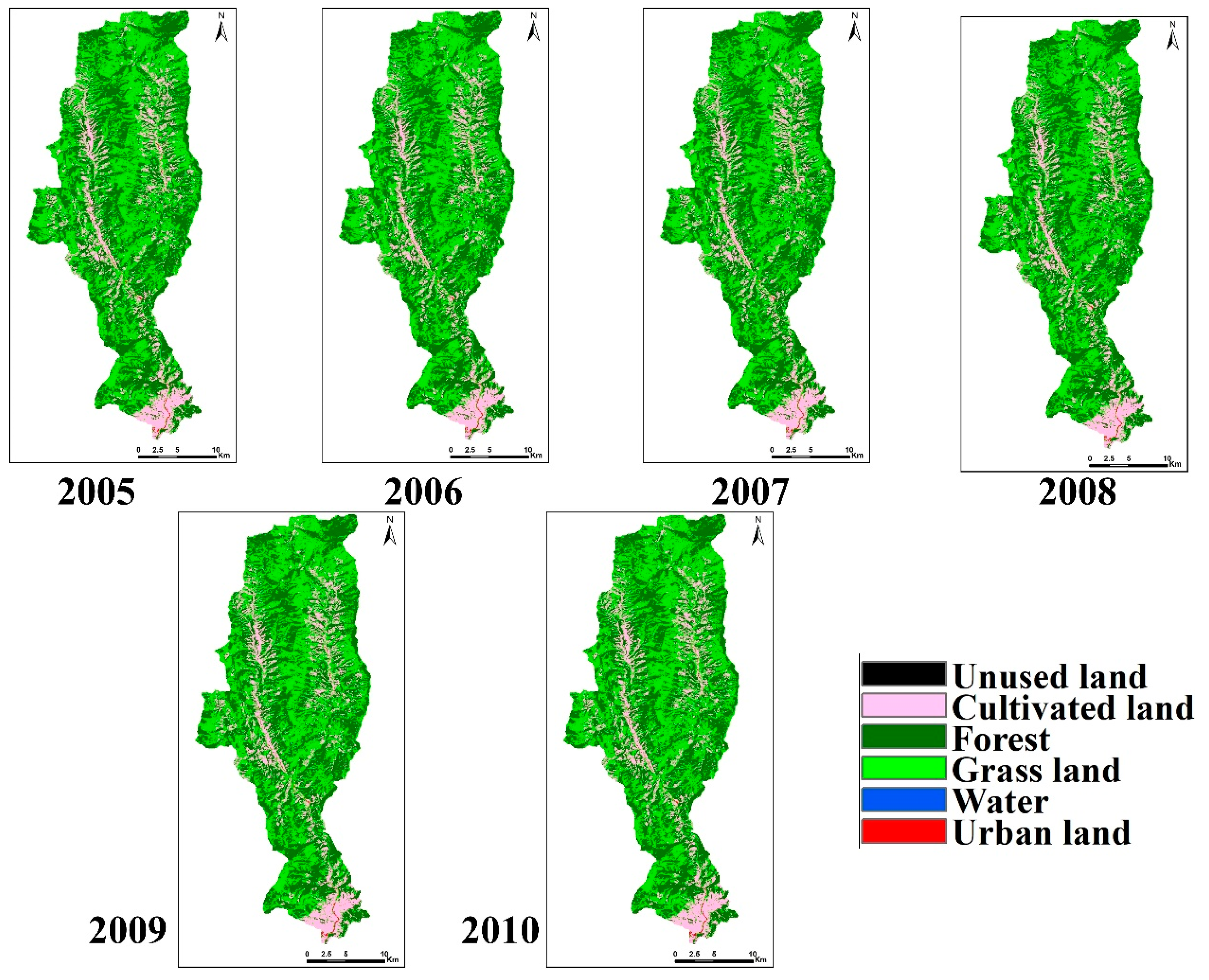
3.1. Hydrological Characteristics and Land Use Change in the Study Area

The consistency and stability of the basin’s hydrology impacted the simulation results of the coupled model. Climate and land use change are two important factors in a coupled model’s consistency and stability [46,97], so studies of land use and climate in the study area are significant for subsequent analyses of the flood simulation.
Climate change was found to have a significant impact on the relationship between rainfall and runoff in the basin. The temperature distribution in the Zhaojue river basin during the study period is shown in Figure 5a. We found that the temperature of the basin significantly varied from −10.0 to 20 °C, with a hot summer and cold winter. The annual average temperature was around 10 °C for many years. The highest temperature occurred around July, generally 19.0 °C, and the lowest temperature occurred around January, generally −5.0 °C. The temperature change correlated with the hydrological characteristics of the study area. The annual hydrological characteristics of the basin during the study period are shown in Figure 5b. The mean annual rainfall was about 1400 mm, the mean runoff depth was 600 mm, and the runoff coefficient was relatively stable at about 0.45. These results further suggest that the study area had significant hydrological consistency during the study period.
Land use change has an important impact on the flood process at the basin scale. The area percentages of land use in the basin during the study period are shown in Table 4, and the maps of land use are shown in Figure 6. There are six types of land use in the study area, the main ones being cultivated land, grassland, and forest, which account for over 99% in total, and it is worth noting that the degree of land use change is not obvious. Consequently, land use changes will have little impact on the consistency of the hydrology, which is beneficial for our research.

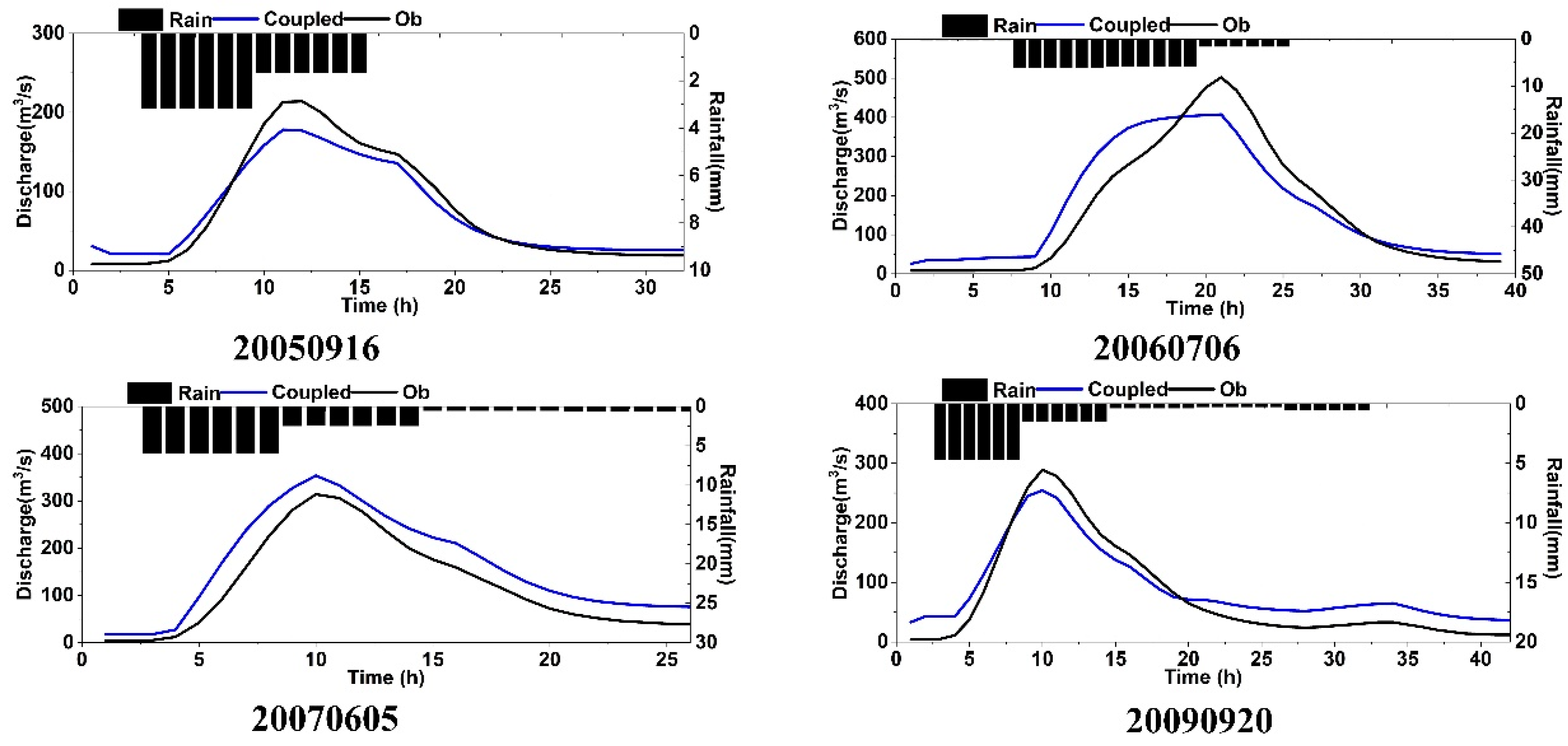
3.2. Performance Assessment of Coupled Model for Real Flood Events

The performance of the coupled model was evaluated by analyzing the discharge process at the outlet gauging station, as indicated in Section 2.4. Considering the availability and consistency of hydrological data, six flood events were selected for model calibration and four flood events were used for model validation. The results of the coupled model are presented in Table 5.
According to these statistical indicators, NSE values were generally within an acceptable range between 0.48 and 0.95, with an average value of 0.79 in all flood events. Event no. 20050916 presented the highest values, whereas event no. 20100821 had the lowest values due to the complex topography and rainfall distribution [46]. The absolute RE in the calibration period ranged between 4.02% and 33.95%, with an average value of 18.17%, and between 1.22% and 81.92% in the validation period. The PE indices were rather satisfactory, with low error rates (within ±20%) in most events (except for event no. 20050707 due to antecedent precipitation). The investigation of the arrival time of the flood peak revealed that the model accurately simulated the timing of the confluence. A coupled model can simulate the peak discharge and routing process in enough detail to comprehensively consider the impacts of land use on flooding [98], so the arrival time of the flood peak from the coupled model was well matched with the observations.
In addition to the statistical indicators, simulated hydrographs from the coupled model were plotted with the observed discharge hydrographs to compare the observed and simulated discharge processes (Figure 7). Figure 7 shows that the simulated stage hydrograph agreed well with that observed at the outlet of the basin. The agreement indicates that the developed equation and method could adequately describe the observed surface runoff process. However, the peak discharges were underestimated for most of the flood events, which may have been caused by the infiltration excess runoff due to topography [81]. It is also noteworthy that the discharges were overestimated for the low flow; this is due to agricultural storage (15% of all land, Table 4) and the depression storage or the antecedent precipitation error [99]. During storms, the coupled model could accurately simulate the peak flow and the arrival time in most flood events, demonstrating the strengths of the hydraulic model for confluence.
In summary, although some simulated events (event nos. 20050707 and 20100821) had certain errors, the overall accuracy of the results based on the evaluation criteria in Section 2.4 was within an acceptable range. As such, the coupled model can be applied in flood risk assessment.

3.3. Flood Risk Response of Different Land Uses

A flood risk management method is essential for protecting downstream residents. This method can be used to prepare flood risk maps in order to analyze the impact of land use on the flood process [100,101,102]. These maps could provide more decision support for land use planners, authorities, and governments to develop appropriate policy responses to mitigate or prevent potential damage due to flooding [33].
For this paper, we selected the flood event 20060706 as an example for flood risk analysis because it showed a typical flow distribution. We set the threshold of inundated depth to 0.01 m. First, we investigated how the inundation dynamics evolved over time, and water depth maps at various time points are presented in Figure 8. The overland runoff flowed from the hillside to the channel and eventually along the channel. With the increase in rainfall intensity, the scope of surface flow also expanded, and the coverage of water flow widened (from 5 to 18 h). When the rainfall approached the peak moment (9 h), the inundation extent obviously increased. These results show that the spatial distribution of flood behavior calculated with the coupled model could be used for flooding mitigation and land use planning.
Based on the flood evolution process, the changes in the flood inundation areas and average water depth were calculated and are presented in Figure 9. Both of them gradually increased over time (Figure 9); at 20 h (near maximum cumulative rainfall), flood inundation areas reached their peak, accounting for 1.3% and reaching 8.45 km2. As can be seen in the inundation extent information shown in Figure 8, the roads close to the river (as well as cultivated and urban land) contributed the most to the inundation areas. The results indicate that these risk loci were prone to flooding during significantly heavy rainfall. After 20 h, the spatial distribution of flooded areas was basically stable, indicating that the duration was long and the damage area was relatively large.
The maximum water depth is an important indicator for flood evaluation and hazard estimation. In this study, the maximum water depth was analyzed, and the maps of it are presented in Figure 10a (their zoomed-in views are also illustrated in Figure 10b,c). The maximum water depth was less than 1 m in most areas, and the maximum value was 1.22 m (Figure 10a). Taken as a whole, extensive inundation could be observed in main roads, intersections, and dense residential quarters (Figure 10b,c). Heavy rainstorms within these areas will cause more severe, more intense, and longer floods. Even worse, Zhaojue county has a low elevation and is located at the outlet of the basin, so flooding will pose significant threats to people’s lives and property when rainstorms occur. Therefore, we recommend implementing river regulation projects and structural reinforcement in the upper reaches of Zhaojue river.
Flood risk was divided into four categories based on water depth: 0.05–0.1 m, 0.1–0.2 m, 0.2–0.4 m, and >0.4 m. The inundation areas and percentages under different levels were calculated and are shown in Table 6. The results show that a total area of 9.17 km2 (about 1.88% of the total area) was at risk of flooding. Although the overall proportion was not large, it was mostly in the landslide-prone areas, in which the harm caused was significant. In addition, residential areas and cultivated land accounted for a large proportion in the inundation extent (Figure 10a), followed by roads, thus allowing for serious disasters.
The modeled velocity over highly irregular topography was of significant interest as it could clearly reflect the impact of the topography on the flood flow. The flow velocity in the basin was found to vary between 0.01 and 1.0 m/s—mostly below 0.1 m/s—and sometimes between 0.1 and 0.3 m/s (Figure 11a). The velocities in the narrow reach of the channel were higher than those in the wider reach. Furthermore, no non-physical (unrealistically high) velocity was discerned, which reflected the satisfactory performance of the present model from the numerical perspective. “Derivative” metrics, such as shear stress and vorticity, could be derived from velocity information, which would be helpful for understanding the effects of land use and basin hydrology on soil erosion and sediment transport. A map of the arrival time of the maximum water depth (relative to initial time of the event) is presented in Figure 11b, which clearly shows the flow process from the hillside to the river.
Furthermore, some high-risk sites are shown in Figure 12, which shows that the risk points were mostly located in the downstream river channel (Figure 12b) and surrounding villages (Figure 12c). The arrival time of the maximum water depth is an important variable, providing a reference for disaster relief time and relief route—for example, transferring people before a certain inundation depth. Hence, it is recommended to prioritize the evacuation of large numbers of people ahead of the arrival of some extreme flooding using information gained from the arrival time map (Figure 11b). Overall, the diverse spatial patterns of the changes in flood occurrence reflect various aspects of rainfall intensity, topography, and land use over the basin, demonstrating that the results were reasonable.

4. Discussions

4.1. The Coupled Hydrological–Hydraulic Model and Flood Process

Although the authors of numerous studies have investigated the flood process by integrating hydrological and 2D models (e.g., [103,104,105]), it is relatively rare for lumped rainfall–runoff (RR) models to be coupled with hydraulic models at the basin scale, even though some scholars have called for more research into this topic [77]. It is still a significant challenge to allocate overland flow in lumped RR to the boundary of a hydraulic model (usually uniform distribution [61,91,106]). In our coupled approach, the application effect of the XAJ model in runoff production has widely been proven possible [83,94], and 2D models have also been successfully adopted to assess anthropogenic impacts on the flood process at the basin scale [107,108,109]. Therefore, we are confident in the coupling method of this paper. Furthermore, compared to previous studies, we have expanded the scope of application (not only in experimental conditions [110]) and also addressed the computational domain problem with our coupled model [76,77].
Accordingly, the proposed coupled model has demonstrated its value in our study area. The results (Table 5) indicate the model’s strong performance during the calibration and validation periods, which is in line with related research with similar methods [54,105]. In terms of the NSE value (average NSE = 0.79), the results showed an acceptable accuracy that was consistent with other studies (e.g., average NSE = 0.80 in [58]). Compared to a single hydrological model (e.g., average NSE = 0.73 in Longchangqiao station, 0.65 in Huangguoshu station, and 0.68 in Huangmaocun station in [47]), the coupled model reported in this paper showed considerable improvements. Regarding the arrival time (average Δ T = 1.2), the performance of our model was similar to or better than that of other studies (e.g., [71,98]). Wang et al. adopted the same coupled model to simulate floods at different magnitudes, but the results presented in this paper are better in terms of small and medium flood events due to the more precise surface flow assignment in our work (the surface flow was homogenized in that study) [91]. Similarly, the results of this study are better than those of our previous research with the same model [61] due to the fact that the study area of the previous research contained many dams that the coupled model failed to consider. However, we still observed some errors in our study (20100821 in Table 5) due to errors in the meteorological data or runoff production caused by the complex topography [81,111].

4.2. The Impact of Land Use and Topography on Flood Process

Munar et al. reported that the coupled model is a promising approach to investigate the impact of land use and topography on the flood process [57]. Related scholars have also proposed the necessity of applying the coupled model in flood research with complex terrains [88,112]. Therefore, we explored the relationship between topography and the flood process. Our flood evolution map (Figure 8) showed that the flow movement was basically consistent with the terrain. Additionally, due to the lower terrain, downstream areas were found to be more vulnerable to flooding than upstream areas (Figure 10), which puts more pressure on the flood control of downstream cities. These findings are consistent with those of Possa [113].
Land use was found to have significant impacts on runoff production and flood routing through different forms. The velocity map (Figure 11a) showed that different land uses had different effects on the dynamics of floods: the flow velocity sequentially increased in the vegetation, cultivated, and building zones. This phenomenon indicated that the interception rate of vegetation to flooding was high and that the urban land reduced the convergence time. The maximum water depth map (Figure 10) showed the impact of different land uses on floods: the vegetation zones were hardly submerged (less than 0.01 m), indicating the weakening effect of vegetation on flooding. However, there were more flood risk points in the urban area (Figure 10 and Figure 12), indicating that urbanization will lead to the aggravation of rainstorms and flood intensity.

4.3. Strengths and Weaknesses

The coupled model proposed in this paper combines the advantages of both hydrological and hydraulic models and could be used to simulate an entire basin. The backwater problem (i.e., the effects of building and tree heights) mentioned in previous research [114,115] has been addressed as efficiently as possible by FABDEM [116]. Due to the unevenness of underlying surfaces (microtopography), overland flow depths and speeds are highly variable and discontinuous in space and time [89]. FABDEM allowed us to significantly improve the consistency of the model and will allow for better representation of elevation, avoiding the “nonflow phenomenon” that occurs in some grids at low runoff production rates. Furthermore, in terms of accuracy, FABDEM is superior to existing elevation products, and its properties are well suited to hydraulic simulations [116].
There are three types of coupling: full coupling, internal coupling, and external coupling [117]. To facilitate such model selection and further promote the coupling of hydrological and hydraulic models, the proposed coupled model was designed with external coupling, which can incorporate more models to replace the XAJ model in an expandable way. Additionally, external coupling is the simplest and most common approach that can be highly extensible and combined without modifying the code of each model. We believe that we were able to better understand the flood process by joining the locally best performing hydrological and hydraulic models.
Despite these advantages, the coupled model has several limitations.
Begnudelli et al. pointed out that roughness has a vital role in routing time [118], and previous research has suggested that the Manning coefficient is a more sensitive parameter [98]. Hence, the impact of land use on roughness in our work requires further study. Additionally, Manning’s coefficient is related to terrain and water depth [89], so the construction of a comprehensive solution for the Manning coefficient would be helpful to improve the model’s performance. Furthermore, although the agreement between the coupled model and the observed discharge at the outlet was satisfactory, there is still a need to evaluate the velocities and water depths. This will greatly benefit from the linking of more data sources, such as the Surface Water and Ocean Topography (SWOT) mission or more detailed data sources (e.g., radar or more gauge stations) [119].
In addition, the scale problem of flood simulation needs to be seriously considered [120]. Coarser resolution datasets may impact model applications [57]. Although the resolution of the dataset used in this paper was consistent with that of previous studies [19,91,121] and can be used for flood simulation, its impact on the model’s performance was not considered; we need to further study the model’s performance under different resolutions. Furthermore, the uncertainty of input data impacts model results, and rainfall is considered the most important source of uncertainty [122]. Accordingly, to decrease the impact caused by rainfall uncertainty, the average rainfall of three rainfall stations was used to represent the rainfall distribution in this study. Topography is another source of uncertainty; although FABDEM was adopted to characterize the topographic changes in the basin, which is helpful for flood simulation [116], its application effect needs further evaluation.

5. Conclusions

The impact of land use on the hydrological process is particularly pronounced. In this paper, we have presented a systematic approach based on the effective coupling of hydrological and hydraulic models to assess the effect of land use on flood risk. In the coupled model, the XAJ model was adopted to generate overland flow and the floodplain evolution was implemented by a 2D hydraulic model. A strong agreement between the simulated and measured discharge results was achieved. This integrated approach could be a useful strategy for flood and land use management and could complement existing flood planning tools in southwestern China. The key findings are summarized as follows.
(1)
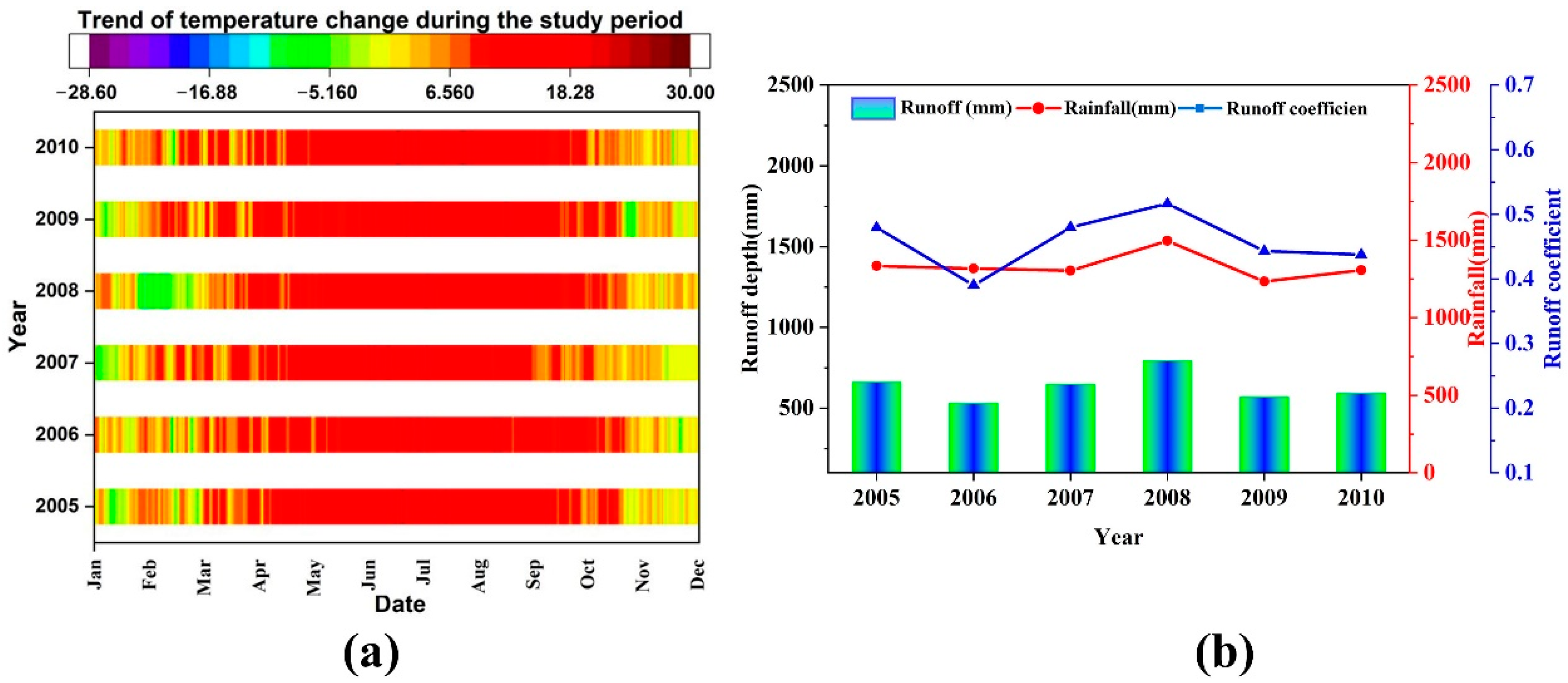
According to the analysis of hydrological characteristics (Section 3.1), it was concluded that the hydraulic and hydrologic features did not significantly change during the study period. The relationship between rainfall and runoff had a significant consistency. This was beneficial for coupled model application.
(2)
The results (Section 3.2) showed that the coupled model had a strong applicability to the basin in southwestern China. The model was able to reproduce observed hydrographs, and discharge was well simulated (Table 5 and Figure 7). We found that 80% of the flood events had an NSE value exceeding 0.70. In particular, the time of concentration and peak flows were well simulated: the simulated peak time matched well with the observed values with an error of less than ±3 h, and the PE values of most flood events were within 20%.
(3)
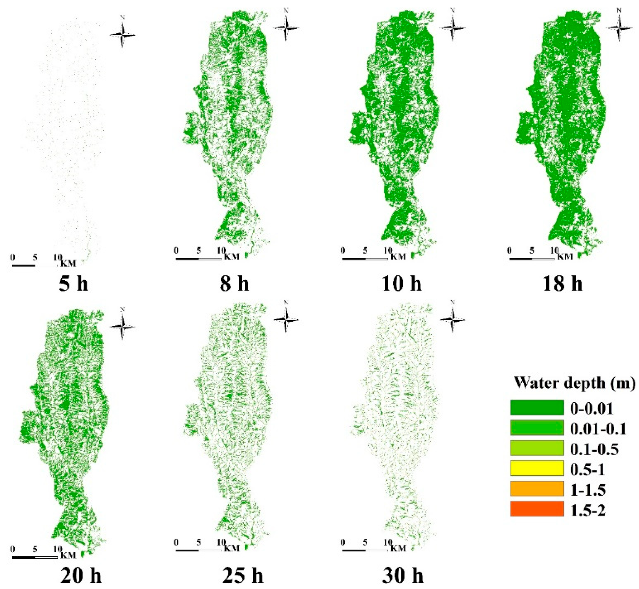
A unique advantage of the coupled model is that in addition to the flow hydrograph, it offers inundated area, water depth, and velocity information that is fundamental for reliable flood risk analysis. Our flood risk analysis results (Section 3.3) suggested that the coupled model is suitable for simulating inundation and could provide an important tool for flood management to reduce damage in terms of lives and property in the Zhaojue river basin.
(4)
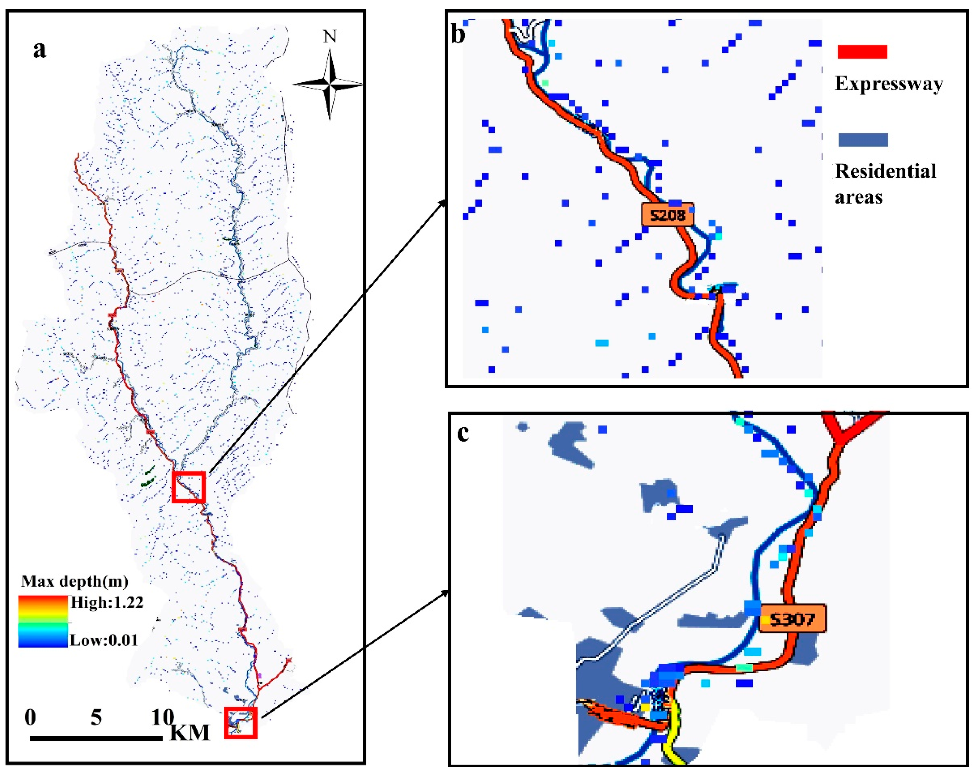
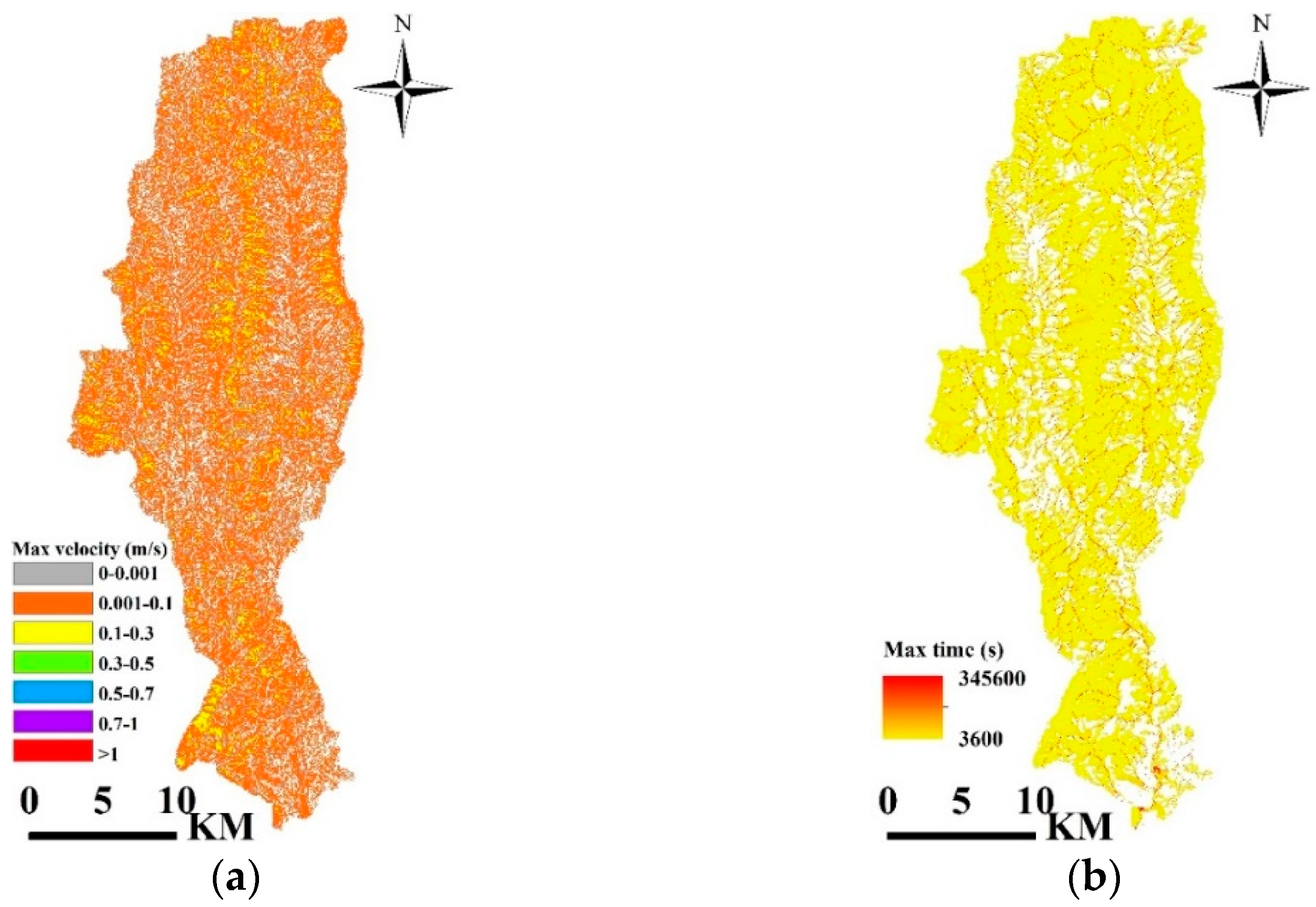
The flood risk maps (Section 3.3) indicated that topography and land use played the most major roles in flood wave attenuation and delay. The flow velocity map (Figure 12a) showed that different land use types had different impacts on flood process. The order of flow velocity was as follows: forest < grassland < cultivated land < urban land. This order also reflected the degree of interception of floods by different land use types. These results showed that the strengthening of land management has played an important role in reducing flood risk.
Although our preliminary test demonstrates the relationship between the flood process and land use, there are still many questions to be addressed. Ongoing research can focus on the spatial verification of flood inundation extents with more measured data or radar data. Additionally, the Manning coefficient adopted in this paper was calculated from relevant research results; thus, the calculation of more accurate Manning coefficients to improve the coupled model’s performance is worth exploring. Furthermore, the effect of the resolution of remote sensing data on the coupled model’s results is also worth investigating.

Author Contributions

Conceptualization, C.X. and H.F.; methodology, C.X. and H.F.; software, C.X.; validation, C.X., J.Y. and L.W.; formal analysis, C.X. and H.F.; investigation, H.F.; resources, J.Y.; data curation, L.W. and H.F.; writing—original draft preparation, C.X., H.F., and J.Y.; writing—review and editing, L.W.; visualization, J.Y.; supervision, H.F.; project administration, H.F.; funding acquisition, H.F. All authors have read and agreed to the published version of the manuscript.

Funding

This research was funded by the Major Science and Technology Program for Water Pollution Control and Treatment (Grant No. 2014ZX07203-008).

Institutional Review Board Statement

Not applicable.

Informed Consent Statement

Not applicable.

Data Availability Statement

All data generated or analyzed during this study are included in this article, and the datasets used or analyzed during the current study are available from the corresponding authors on reasonable request.

Acknowledgments

The authors would like to acknowledge Xiaoliu Yang of Peking University, China, for his theoretical support and guidance.

Conflicts of Interest

The authors declare no conflict of interest.

References

  1. Wang, Y.T.; Chen, A.S.; Fu, G.T.; Djordjevic, S.; Zhang, C.; Savic, D.A. An integrated framework for high-resolution urban flood modelling considering multiple information sources and urban features. Environ. Modell. Softw. 2018, 107, 85–95. [Google Scholar] [CrossRef]
  2. Toosi, A.S.; Calbimonte, G.H.; Nouri, H.; Alaghmand, S. River basin-scale flood hazard assessment using a modified multi-criteria decision analysis approach: A case study. J. Hydrol. 2019, 574, 660–671. [Google Scholar] [CrossRef]
  3. Ceola, S.; Laio, F.; Montanari, A. Satellite nighttime lights reveal increasing human exposure to floods worldwide. Geophys. Res. Lett. 2014, 41, 7184–7190. [Google Scholar] [CrossRef]
  4. Dou, Y.H.; Ye, L.; Gupta, H.V.; Zhang, H.R.; Behrangi, A.; Zhou, H.C. Improved Flood Forecasting in Basins With No Precipitation Stations: Constrained Runoff Correction Using Multiple Satellite Precipitation Products. Water Resour. Res. 2021, 57, e2021WR029682. [Google Scholar] [CrossRef]
  5. Archer, D.R.; Fowler, H.J. Characterising flash flood response to intense rainfall and impacts using historical information and gauged data in Britain. J. Flood Risk Manag. 2018, 11, S121–S133. [Google Scholar] [CrossRef]
  6. Breinl, K.; Lun, D.; Muller-Thomy, H.; Bloschl, G. Understanding the relationship between rainfall and flood probabilities through combined intensity-duration-frequency analysis. J. Hydrol. 2021, 602, 126759. [Google Scholar] [CrossRef]
  7. Feng, B.Y.; Zhang, Y.; Bourke, R. Urbanization impacts on flood risks based on urban growth data and coupled flood models. Nat. Hazards 2021, 106, 613–627. [Google Scholar] [CrossRef]
  8. Smith, A.; Bates, P.D.; Wing, O.; Sampson, C.; Quinn, N.; Neal, J. New estimates of flood exposure in developing countries using high-resolution population data. Nat. Commun. 2019, 10, 1814. [Google Scholar] [CrossRef] [Green Version]
  9. Kesikoglu, M.H.; Atasever, U.H.; Dadaser-Celik, F.; Ozkan, C. Performance of ANN, SVM and MLH techniques for land use/cover change detection at Sultan Marshes wetland, Turkey. Water Sci. Technol. 2019, 80, 466–477. [Google Scholar] [CrossRef]
  10. Alfieri, L.; Bisselink, B.; Dottori, F.; Naumann, G.; de Roo, A.; Salamon, P.; Wyser, K.; Feyen, L. Global projections of river flood risk in a warmer world. Earths Future 2017, 5, 171–182. [Google Scholar] [CrossRef]
  11. Fang, G.H.; Yuan, Y.; Gao, Y.Q.; Huang, X.F.; Guo, Y.X. Assessing the Effects of Urbanization on Flood Events with Urban Agglomeration Polders Type of Flood Control Pattern Using the HEC-HMS Model in the Qinhuai River Basin, China. Water 2018, 10, 1003. [Google Scholar] [CrossRef] [Green Version]
  12. He, B.S.; Huang, X.L.; Ma, M.H.; Chang, Q.R.; Tu, Y.; Li, Q.; Zhang, K.; Hong, Y. Analysis of flash flood disaster characteristics in China from 2011 to 2015. Nat. Hazards 2018, 90, 407–420. [Google Scholar] [CrossRef]
  13. Liu, W.M.; Carling, P.A.; Hu, K.H.; Wang, H.; Zhou, Z.; Zhou, L.Q.; Liu, D.Z.; Lai, Z.P.; Zhang, X.B. Outburst floods in China: A review. Earth-Sci. Rev. 2019, 197, 102895. [Google Scholar] [CrossRef]
  14. Wei, L.; Hu, K.H.; Hu, X.D. Rainfall occurrence and its relation to flood damage in China from 2000 to 2015. J. Mt. Sci. 2018, 15, 2492–2504. [Google Scholar] [CrossRef]
  15. Glas, H.; Jonckheere, M.; Mandal, A.; James-Williamson, S.; De Maeyer, P.; Deruyter, G. A GIS-based tool for flood damage assessment and delineation of a methodology for future risk assessment: Case study for Annotto Bay, Jamaica. Nat. Hazards 2017, 88, 1867–1891. [Google Scholar] [CrossRef]
  16. Handayani, W.; Chigbu, U.E.; Rudiarto, I.; Putri, I.H.S. Urbanization and Increasing Flood Risk in the Northern Coast of Central Java-Indonesia: An Assessment towards Better Land Use Policy and Flood Management. Land 2020, 9, 343. [Google Scholar] [CrossRef]
  17. Diez-Herrero, A.; Garrote, J. Flood Risk Analysis and Assessment, Applications and Uncertainties: A Bibliometric Review. Water 2020, 12, 2050. [Google Scholar] [CrossRef]
  18. Kreibich, H.; Di Baldassarre, G.; Vorogushyn, S.; Aerts, J.C.J.H.; Apel, H.; Aronica, G.T.; Arnbjerg-Nielsen, K.; Bouwer, L.M.; Bubeck, P.; Caloiero, T.; et al. Adaptation to flood risk: Results of international paired flood event studies. Earths Future 2017, 5, 953–965. [Google Scholar] [CrossRef] [Green Version]
  19. Kim, J.; Warnock, A.; Ivanov, V.Y.; Katopodes, N.D. Coupled modeling of hydrologic and hydrodynamic processes including overland and channel flow. Adv. Water Resour. 2012, 37, 104–126. [Google Scholar] [CrossRef]
  20. Attems, M.S.; Thaler, T.; Genovese, E.; Fuchs, S. Implementation of property-level flood risk adaptation (PLFRA) measures: Choices and decisions. Wiley Interdiscip. Rev. Water 2020, 7, e1404. [Google Scholar] [CrossRef] [Green Version]
  21. Costache, R.; Bui, D.T. Identification of areas prone to flash-flood phenomena using multiple-criteria decision-making, bivariate statistics, machine learning and their ensembles. Sci. Total Environ. 2020, 712, 136492. [Google Scholar] [CrossRef] [PubMed]
  22. Wu, X.S.; Wang, Z.L.; Guo, S.L.; Liao, W.L.; Zeng, Z.Y.; Chen, X.H. Scenario-based projections of future urban inundation within a coupled hydrodynamic model framework: A case study in Dongguan City, China. J. Hydrol. 2017, 547, 428–442. [Google Scholar] [CrossRef]
  23. Lowe, R.; Urich, C.; Domingo, N.S.; Mark, O.; Deletic, A.; Arnbjerg-Nielsen, K. Assessment of urban pluvial flood risk and efficiency of adaptation options through simulations-A new generation of urban planning tools. J. Hydrol. 2017, 550, 355–367. [Google Scholar] [CrossRef] [Green Version]
  24. Mehr, A.D.; Kahya, E. A Pareto-optimal moving average multigene genetic programming model for daily streamflow prediction. J. Hydrol. 2017, 549, 603–615. [Google Scholar] [CrossRef]
  25. Fan, C.X.; An, R.D.; Li, J.; Li, K.F.; Deng, Y.; Li, Y. An Approach Based on the Protected Object for Dam-Break Flood Risk Management Exemplified at the Zipingpu Reservoir. Int. J. Environ. Res. Public Health 2019, 16, 3786. [Google Scholar] [CrossRef] [PubMed] [Green Version]
  26. Kumar, N.; Tischbein, B.; Kusche, J.; Beg, M.K.; Bogardi, J.J. Impact of land-use change on the water resources of the Upper Kharun Catchment, Chhattisgarh, India. Reg. Environ. Chang. 2017, 17, 2373–2385. [Google Scholar] [CrossRef]
  27. Hu, S.S.; Fan, Y.Y.; Zhang, T. Assessing the Effect of Land Use Change on Surface Runoff in a Rapidly Urbanized City: A Case Study of the Central Area of Beijing. Land 2020, 9, 17. [Google Scholar] [CrossRef] [Green Version]
  28. Yari, A.; Ardalan, A.; Ostadtaghizadeh, A.; Zarezadeh, Y.; Boubakran, M.S.; Bidarpoor, F.; Rahimiforoushani, A. Underlying factors affecting death due to flood in Iran: A qualitative content analysis. Int. J. Disaster Risk Reduct. 2019, 40, 101258. [Google Scholar] [CrossRef]
  29. Li, B.F.; Shi, X.; Lian, L.S.; Chen, Y.N.; Chen, Z.S.; Sun, X.Y. Quantifying the effects of climate variability, direct and indirect land use change, and human activities on runoff. J. Hydrol. 2020, 584, 124684. [Google Scholar] [CrossRef]
  30. Munoth, P.; Goyal, R. Impacts of land use land cover change on runoff and sediment yield of Upper Tapi River Sub-Basin, India. Int. J. River Basin Manag. 2020, 18, 177–189. [Google Scholar] [CrossRef]
  31. Li, Z.H.; Song, K.Y.; Peng, L. Flood Risk Assessment under Land Use and Climate Change in Wuhan City of the Yangtze River Basin, China. Land 2021, 10, 878. [Google Scholar] [CrossRef]
  32. Junger, L.; Hohensinner, S.; Schroll, K.; Wagner, K.; Seher, W. Land Use in Flood-Prone Areas and Its Significance for Flood Risk Management-A Case Study of Alpine Regions in Austria. Land 2022, 11, 392. [Google Scholar] [CrossRef]
  33. Iacob, O.; Brown, I.; Rowan, J. Natural flood management, land use and climate change trade-offs: The case of Tarland catchment, Scotland. Hydrolog. Sci. J. 2017, 62, 1931–1948. [Google Scholar] [CrossRef] [Green Version]
  34. Zhu, W.B.; Jia, S.F.; Lall, U.; Cao, Q.; Mahmood, R. Relative contribution of climate variability and human activities on the water loss of the Chari/Logone River discharge into Lake Chad: A conceptual and statistical approach. J. Hydrol. 2019, 569, 519–531. [Google Scholar] [CrossRef]
  35. Zheng, H.X.; Zhang, L.; Zhu, R.R.; Liu, C.M.; Sato, Y.; Fukushima, Y. Responses of streamflow to climate and land surface change in the headwaters of the Yellow River Basin. Water Resour. Res. 2009, 45, 7. [Google Scholar] [CrossRef]
  36. Oudin, L.; Salavati, B.; Furusho-Percot, C.; Ribstein, P.; Saadi, M. Hydrological impacts of urbanization at the catchment scale. J. Hydrol. 2018, 559, 774–786. [Google Scholar] [CrossRef] [Green Version]
  37. Zuo, D.P.; Xu, Z.X.; Yao, W.Y.; Jin, S.Y.; Xiao, P.Q.; Ran, D.C. Assessing the effects of changes in land use and climate on runoff and sediment yields from a watershed in the Loess Plateau of China. Sci. Total Environ. 2016, 544, 238–250. [Google Scholar] [CrossRef]
  38. Tong, L.; Dong, J.; Yuan, W.P. Effects of Precipitation and Vegetation Cover on Annual Runoff and Sediment Yield in Northeast China: A Preliminary Analysis. Water Resour. 2020, 47, 491–505. [Google Scholar] [CrossRef]
  39. Liu, J.B.; Gao, G.Y.; Wang, S.; Jiao, L.; Wu, X.; Fu, B.J. The effects of vegetation on runoff and soil loss: Multidimensional structure analysis and scale characteristics. J. Geogr. Sci. 2018, 28, 59–78. [Google Scholar] [CrossRef] [Green Version]
  40. Aghakhani, M.; Nasrabadi, T.; Vafaeinejad, A. Assessment of the Effects of Land Use Scenarios on Watershed Surface Runoff Using Hydrological Modelling. Appl. Ecol. Env. Res. 2018, 16, 2369–2389. [Google Scholar] [CrossRef]
  41. Han, Y.N.; Niu, J.Z.; Xin, Z.B.; Zhang, W.; Zhang, T.L.; Wang, X.L.; Zhang, Y.S. Optimization of land use pattern reduces surface runoff and sediment loss in a Hilly-Gully watershed at the Loess Plateau, China. Forest Syst. 2016, 25, e054. [Google Scholar] [CrossRef] [Green Version]
  42. Ran, J.; Nedovic-Budic, Z. Integrating spatial planning and flood risk management: A new conceptual framework for the spatially integrated policy infrastructure. Comput. Environ. Urban. 2016, 57, 68–79. [Google Scholar] [CrossRef] [Green Version]
  43. Li, C.C.; Cheng, X.T.; Li, N.; Du, X.H.; Yu, Q.; Kan, G.Y. A Framework for Flood Risk Analysis and Benefit Assessment of Flood Control Measures in Urban Areas. Int. J. Env. Res. Pub. Health 2016, 13, 787. [Google Scholar] [CrossRef] [PubMed] [Green Version]
  44. Tasantab, J.C. Beyond the plan: How land use control practices influence flood risk in Sekondi-Takoradi. Jamba-J. Disaster Ris. 2019, 11, 1–9. [Google Scholar] [CrossRef] [Green Version]
  45. Wheater, H.S. Progress in and prospects for fluvial flood modelling. Ser. A Math. Phys. Eng. Sci. 2002, 360, 1409–1431. [Google Scholar] [CrossRef] [PubMed]
  46. Zhou, Q.; Chen, L.; Singh, V.P.; Zhou, J.Z.; Chen, X.H.; Xiong, L.H. Rainfall-runoff simulation in karst dominated areas based on a coupled conceptual hydrological model. J. Hydrol. 2019, 573, 524–533. [Google Scholar] [CrossRef]
  47. Zhao, Y.M.; Liao, W.H.; Lei, X.H. Hydrological Simulation for Karst Mountain Areas: A Case Study of Central Guizhou Province. Water 2019, 11, 991. [Google Scholar] [CrossRef] [Green Version]
  48. Mo, C.X.; Wang, Y.F.; Ruan, Y.L.; Qin, J.K.; Zhang, M.S.; Sun, G.K.; Jin, J.L. The effect of karst system occurrence on flood peaks in small watersheds, southwest China. Hydrol. Res. 2021, 52, 305–322. [Google Scholar] [CrossRef]
  49. Guo, X.M.; Li, T.Y.; He, B.H.; He, X.R.; Yao, Y. Effects of land disturbance on runoff and sediment yield after natural rainfall events in southwestern China. Environ. Sci. Pollut. Res. 2017, 24, 9259–9268. [Google Scholar] [CrossRef] [PubMed]
  50. Zhao, Y.J.; Yang, N.; Wei, Y.P.; Hu, B.; Cao, Q.Z.; Tong, K.; Liang, Y.L. Eight Hundred Years of Drought and Flood Disasters and Precipitation Sequence Reconstruction in Wuzhou City, Southwest China. Water 2019, 11, 219. [Google Scholar] [CrossRef] [Green Version]
  51. Zounemat-Kermani, M.; Matta, E.; Cominola, A.; Xia, X.L.; Zhang, Q.; Liang, Q.H.; Hinkelmann, R. Neurocomputing in surface water hydrology and hydraulics: A review of two decades retrospective, current status and future prospects. J. Hydrol. 2020, 588, 125085. [Google Scholar] [CrossRef]
  52. Shin, S.; Pokhrel, Y.; Yamazaki, D.; Huang, X.D.; Torbick, N.; Qi, J.G.; Pattanakiat, S.; Thanh, N.D.; Tuan, N.D. High Resolution Modeling of River-Floodplain-Reservoir Inundation Dynamics in the Mekong River Basin. Water Resour. Res. 2020, 56, e2019WR026449. [Google Scholar] [CrossRef]
  53. Schumann, G.J.P.; Neal, J.C.; Voisin, N.; Andreadis, K.M.; Pappenberger, F.; Phanthuwongpakdee, N.; Hall, A.C.; Bates, P.D. A first large-scale flood inundation forecasting model. Water Resour. Res. 2013, 49, 6248–6257. [Google Scholar] [CrossRef]
  54. Wang, J.; Yun, X.B.; Pokhrel, Y.; Yamazaki, D.; Zhao, Q.D.; Chen, A.F.; Tang, Q.H. Modeling Daily Floods in the Lancang-Mekong River Basin Using an Improved Hydrological-Hydrodynamic Model. Water Resour. Res. 2021, 57, e2021WR029734. [Google Scholar] [CrossRef]
  55. Zischg, A.P.; Felder, G.; Mosimann, M.; Rothlisberger, V.; Weingartner, R. Extending coupled hydrological-hydraulic model chains with a surrogate model for the estimation of flood losses. Environ. Modell. Softw. 2018, 108, 174–185. [Google Scholar] [CrossRef]
  56. Senent-Aparicio, J.; Lopez-Ballesteros, A.; Nielsen, A.; Trolle, D. A holistic approach for determining the hydrology of the mar menor coastal lagoon by combining hydrological & hydrodynamic models. J. Hydrol. 2021, 603, 127150. [Google Scholar] [CrossRef]
  57. Munar, A.M.; Cavalcanti, J.R.; Bravo, J.M.; Fan, F.M.; da Motta-Marques, D.; Fragos, C.R. Coupling large-scale hydrological and hydrodynamic modeling: Toward a better comprehension of watershed-shallow lake processes. J. Hydrol. 2018, 564, 424–441. [Google Scholar] [CrossRef]
  58. Zhang, K.; Shalehy, M.H.; Ezaz, G.T.; Chakraborty, A.; Mohib, K.M.; Liu, L.X. An integrated flood risk assessment approach based on coupled hydrological-hydraulic modeling and bottom-up hazard vulnerability analysis. Environ. Modell. Softw. 2022, 148, 105279. [Google Scholar] [CrossRef]
  59. Nogherotto, R.; Fantini, A.; Raffaele, F.; Di Sante, F.; Dottori, F.; Coppola, E.; Giorgi, F. A combined hydrological and hydraulic modelling approach for the flood hazard mapping of the Po river basin. J. Flood Risk Manag. 2022, 15, e12755. [Google Scholar] [CrossRef]
  60. Chen, M.Y.; Li, Z.; Gao, S.; Luo, X.Y.; Wing, O.E.J.; Shen, X.Y.; Gourley, J.J.; Kolar, R.L.; Hong, Y. A Comprehensive Flood Inundation Mapping for Hurricane Harvey Using an Integrated Hydrological and Hydraulic Model. J. Hydrometeorol. 2021, 22, 1713–1726. [Google Scholar] [CrossRef]
  61. Xu, C.W.; Han, Z.Y.; Fu, H. Remote Sensing and Hydrologic-Hydrodynamic Modeling Integrated Approach for Rainfall-Runoff Simulation in Farm Dam Dominated Basin. Front. Environ. Sci. 2022, 9, 672. [Google Scholar] [CrossRef]
  62. Lai, X.J.; Jiang, J.H.; Liang, Q.H.; Huang, Q. Large-scale hydrodynamic modeling of the middle Yangtze River Basin with complex river-lake interactions. J. Hydrol. 2013, 492, 228–243. [Google Scholar] [CrossRef]
  63. Paiva, R.C.D.; Collischonn, W.; Tucci, C.E.M. Large scale hydrologic and hydrodynamic modeling using limited data and a GIS based approach. J. Hydrol. 2011, 406, 170–181. [Google Scholar] [CrossRef]
  64. Yin, J.; Yu, D.P.; Yin, Z.N.; Wang, J.; Xu, S.Y. Multiple scenario analyses of Huangpu River flooding using a 1D/2D coupled flood inundation model. Nat. Hazards 2013, 66, 577–589. [Google Scholar] [CrossRef]
  65. Lian, Y.Q.; Chan, I.C.; Singh, J.; Demissie, M.; Knapp, V.; Xie, H. Coupling of hydrologic and hydraulic models for the Illinois River Basin. J. Hydrol. 2007, 344, 210–222. [Google Scholar] [CrossRef]
  66. Barthelemy, S.; Ricci, S.; Morel, T.; Goutal, N.; Le Pape, E.; Zaoui, F. On operational flood forecasting system involving 1D/2D coupled hydraulic model and data assimilation. J. Hydrol. 2018, 562, 623–634. [Google Scholar] [CrossRef]
  67. Hoch, J.M.; Neal, J.C.; Baart, F.; van Beek, R.; Winsemius, H.C.; Bates, P.D.; Bierkens, M.F.P. GLOFRIM v1.0-A globally applicable computational framework for integrated hydrological-hydrodynamic modelling. Geosci. Model. Dev. 2017, 10, 3913–3929. [Google Scholar] [CrossRef] [Green Version]
  68. Grimaldi, S.; Petroselli, A.; Arcangeletti, E.; Nardi, F. Flood mapping in ungauged basins using fully continuous hydrologic-hydraulic modeling. J. Hydrol. 2013, 487, 39–47. [Google Scholar] [CrossRef]
  69. Emmanuel, I.; Andrieu, H.; Leblois, E.; Janey, N.; Payrastre, O. Influence of rainfall spatial variability on rainfall-runoff modelling: Benefit of a simulation approach? J. Hydrol. 2015, 531, 337–348. [Google Scholar] [CrossRef]
  70. Chavarri, E.; Crave, A.; Bonnet, M.P.; Mejia, A.; Da Silva, J.S.; Guyot, J.L. Hydrodynamic modelling of the Amazon River: Factors of uncertainty. J. South Am. Earth Sci. 2013, 44, 94–103. [Google Scholar] [CrossRef]
  71. Parvaze, S.; Khan, J.N.; Kumar, R.; Allaie, S.P. Flood forecasting in Jhelum river basin using integrated hydrological and hydraulic modeling approach with a real-time updating procedure. Clim. Dynam. 2022, 2022, 1–25. [Google Scholar] [CrossRef]
  72. Cao, Z.; Wang, X.; Pender, G.; Zhang, S. Hydrodynamic modelling in support of flash flood warning. Water Manag. 2010, 163, 327–340. [Google Scholar] [CrossRef]
  73. Li, H.; Beldring, S.; Xu, C.Y. Stability of model performance and parameter values on two catchments facing changes in climatic conditions. Hydrolog. Sci. J. 2015, 60, 1317–1330. [Google Scholar] [CrossRef] [Green Version]
  74. Costabile, P.; Costanzo, C.; Macchione, F. A storm event watershed model for surface runoff based on 2D fully dynamic wave equations. Hydrol. Process. 2013, 27, 554–569. [Google Scholar] [CrossRef]
  75. Zhang, L.; Lu, J.Z.; Chen, X.L.; Liang, D.; Fu, X.K.; Sauvage, S.; Perez, J.M.S. Stream flow simulation and verification in ungauged zones by coupling hydrological and hydrodynamic models: A case study of the Poyang Lake ungauged zone. Hydrol. Earth Syst. Sci. 2017, 21, 5847–5861. [Google Scholar] [CrossRef] [Green Version]
  76. Laganier, O.; Ayral, P.A.; Salze, D.; Sauvagnargues, S. A coupling of hydrologic and hydraulic models appropriate for the fast floods of the Gardon River basin (France). Nat. Hazards Earth Syst. Sci. 2014, 14, 2899–2920. [Google Scholar] [CrossRef] [Green Version]
  77. Lerat, J.; Perrin, C.; Andreassian, V.; Loumagne, C.; Ribstein, P. Towards robust methods to couple lumped rainfall-runoff models and hydraulic models: A sensitivity analysis on the Illinois River. J. Hydrol. 2012, 418, 123–135. [Google Scholar] [CrossRef] [Green Version]
  78. Yang, R.W.; Wang, J. Interannual variability of the seesaw mode of the interface between the Indian and East Asian summer monsoons. Clim. Dynam. 2019, 53, 2683–2695. [Google Scholar] [CrossRef]
  79. Li, Z.X.; He, Y.Q.; Wang, P.Y.; Theakstone, W.H.; An, W.L.; Wang, X.F.; Lu, A.G.; Zhang, W.; Cao, W.H. Changes of daily climate extremes in southwestern China during 1961–2008. Glob. Planet Chang. 2012, 80–81, 255–272. [Google Scholar] [CrossRef]
  80. Liu, M.X.; Xu, X.L.; Sun, A.Y.; Wang, K.L.; Liu, W.; Zhang, X.Y. Is southwestern China experiencing more frequent precipitation extremes? Environ. Res. Lett. 2014, 9, 064002. [Google Scholar] [CrossRef] [Green Version]
  81. Chen, X.; Zhang, Z.C.; Chen, X.H.; Shi, P. The impact of land use and land cover changes on soil moisture and hydraulic conductivity along the karst hillslopes of southwest China. Environ. Earth Sci. 2009, 59, 811–820. [Google Scholar] [CrossRef]
  82. Liu, M.X.; Xu, X.L.; Sun, A. Decreasing spatial variability in precipitation extremes in southwestern China and the local/large-scale influencing factors. J. Geophys. Res.-Atmos. 2015, 120, 6480–6488. [Google Scholar] [CrossRef]
  83. Zhao, R.J. The Xinanjiang Model Applied in China. J. Hydrol. 1992, 135, 371–381. [Google Scholar] [CrossRef]
  84. Lu, H.S.; Hou, T.; Horton, R.; Zhu, Y.H.; Chen, X.; Jia, Y.W.; Wang, W.; Fu, X.L. The streamflow estimation using the Xinanjiang rainfall runoff model and dual state-parameter estimation method. J. Hydrol. 2013, 480, 102–114. [Google Scholar] [CrossRef]
  85. Monajemi, P.; Khaleghi, S.; Maleki, S. Derivation of instantaneous unit hydrographs using linear reservoir models. Hydrol. Res. 2021, 52, 339–355. [Google Scholar] [CrossRef]
  86. Meehan, P.J. Flood Routing by the Muskingum Method-Comments. J. Hydrol. 1979, 41, 167–168. [Google Scholar] [CrossRef]
  87. Hou, J.M.; Simons, F.; Liang, Q.H.; Hinkelmann, R. An improved hydrostatic reconstruction method for shallow water model. J. Hydraul. Res. 2014, 52, 432–439. [Google Scholar] [CrossRef]
  88. Liang, Q.H.; Borthwick, A.G.L. Adaptive quadtree simulation of shallow flows with wet-dry fronts over complex topography. Comput. Fluids 2009, 38, 221–234. [Google Scholar] [CrossRef]
  89. Fiedler, F.R.; Ramirez, J.A. A numerical method for simulating discontinuous shallow flow over an infiltrating surface. Int. J. Numer. Methods Fluids 2000, 32, 219–240. [Google Scholar] [CrossRef]
  90. Wagner, P.D.; Fiener, P.; Wilken, F.; Kumar, S.; Schneider, K. Comparison and evaluation of spatial interpolation schemes for daily rainfall in data scarce regions. J. Hydrol. 2012, 464, 388–400. [Google Scholar] [CrossRef]
  91. Wang, Y.L.; Yang, X.L. A Coupled Hydrologic-Hydraulic Model (XAJ-HiPIMS) for Flood Simulation. Water 2020, 12, 1288. [Google Scholar] [CrossRef]
  92. Goegebeur, M.; Pauwels, V.R.N. Improvement of the PEST parameter estimation algorithm through Extended Kalman Filtering. J. Hydrol. 2007, 337, 436–451. [Google Scholar] [CrossRef]
  93. Li, H.X.; Zhang, Y.Q.; Chiew, F.H.S.; Xu, S.G. Predicting runoff in ungauged catchments by using Xinanjiang model with MODIS leaf area index. J. Hydrol. 2009, 370, 155–162. [Google Scholar] [CrossRef]
  94. Yao, C.; Zhang, K.; Yu, Z.B.; Li, Z.J.; Li, Q.L. Improving the flood prediction capability of the Xinanjiang model in ungauged nested catchments by coupling it with the geomorphologic instantaneous unit hydrograph. J. Hydrol. 2014, 517, 1035–1048. [Google Scholar] [CrossRef]
  95. Lin, K.R.; Lv, F.S.; Chen, L.; Singh, V.P.; Zhang, Q.; Chen, X.H. Xinanjiang model combined with Curve Number to simulate the effect of land use change on environmental flow. J. Hydrol. 2014, 519, 3142–3152. [Google Scholar] [CrossRef]
  96. Moriasi, D.N.; Gitau, M.W.; Pai, N.; Daggupati, P. Hydrologic and Water Quality Models: Performance Measures and Evaluation Criteria. Trans. ASABE 2015, 58, 1763–1785. [Google Scholar] [CrossRef] [Green Version]
  97. McGrane, S.J. Impacts of urbanisation on hydrological and water quality dynamics, and urban water management: A review. Hydrolog. Sci. J. 2016, 61, 2295–2311. [Google Scholar] [CrossRef]
  98. Nguyen, P.; Thorstensen, A.; Sorooshian, S.; Hsu, K.L.; AghaKouchak, A.; Sanders, B.; Koren, V.; Cui, Z.T.; Smith, M. A high resolution coupled hydrologic-hydraulic model (HiResFlood-UCI) for flash flood modeling. J. Hydrol. 2016, 541, 401–420. [Google Scholar] [CrossRef] [Green Version]
  99. Frei, S.; Fleckenstein, J.H. Representing effects of micro-topography on runoff generation and sub-surface flow patterns by using superficial rill/depression storage height variations. Environ. Modell. Softw. 2014, 52, 5–18. [Google Scholar] [CrossRef]
  100. Tyler, J.; Sadiq, A.A.; Noonan, D.S. A review of the community flood risk management literature in the USA: Lessons for improving community resilience to floods. Nat. Hazards 2019, 96, 1223–1248. [Google Scholar] [CrossRef]
  101. Dieperink, C.; Hegger, D.L.T.; Bakker, M.H.N.; Kundzewicz, Z.W.; Green, C.; Driessen, P.P.J. Recurrent Governance Challenges in the Implementation and Alignment of Flood Risk Management Strategies: A Review. Water Resour. Manag. 2016, 30, 4467–4481. [Google Scholar] [CrossRef] [Green Version]
  102. Komi, K.; Neal, J.; Trigg, M.A.; Diekkruger, B. Modelling of flood hazard extent in data sparse areas: A case study of the Oti River basin, West Africa. J. Hydrol.-Reg. Stud. 2017, 10, 122–132. [Google Scholar] [CrossRef] [Green Version]
  103. Wei, Z.W.; He, X.G.; Zhang, Y.G.; Pan, M.; Sheffield, J.; Peng, L.Q.; Yamazaki, D.; Moiz, A.; Liu, Y.P.; Ikeuchi, K. Identification of uncertainty sources in quasi-global discharge and inundation simulations using satellite-based precipitation products. J. Hydrol. 2020, 589, 125180. [Google Scholar] [CrossRef]
  104. Sindhu, K.; Rao, K.H.V.D. Hydrological and hydrodynamic modeling for flood damage mitigation in Brahmani-Baitarani River Basin, India. Geocarto Int. 2017, 32, 1004–1016. [Google Scholar] [CrossRef]
  105. Cheng, T.; Xu, Z.X.; Yang, H.; Hong, S.Y.; Leitao, J.P. Analysis of Effect of Rainfall Patterns on Urban Flood Process by Coupled Hydrological and Hydrodynamic Modeling. J. Hydrol. Eng. 2020, 25, 04019061. [Google Scholar] [CrossRef]
  106. Huang, W.; Cao, Z.X.; Qi, W.J.; Pender, G.; Zhao, K. Full 2D hydrodynamic modelling of rainfall-induced flash floods. J. Mt. Sci. 2015, 12, 1203–1218. [Google Scholar] [CrossRef]
  107. Wang, Y.L.; Liang, Q.H.; Kesserwani, G.; Hall, J.W. A 2D shallow flow model for practical dam-break simulations. J. Hydraul. Res. 2011, 49, 307–316. [Google Scholar] [CrossRef]
  108. Liang, Q.H.; Smith, L.S. A high-performance integrated hydrodynamic modelling system for urban flood simulations. J. Hydroinform. 2015, 17, 518–533. [Google Scholar] [CrossRef]
  109. Wing, O.E.J.; Bates, P.D.; Neal, J.C.; Sampson, C.C.; Smith, A.M.; Quinn, N.; Shustikova, I.; Domeneghetti, A.; Gilles, D.W.; Goska, R.; et al. A New Automated Method for Improved Flood Defense Representation in Large-Scale Hydraulic Models. Water Resour. Res. 2019, 55, 11007–11034. [Google Scholar] [CrossRef] [Green Version]
  110. Ajayi, A.E.; van de Giesen, N.; Vlek, P. A numerical model for simulating Hortonian overland flow on tropical hillslopes with vegetation elements. Hydrol. Process. 2008, 22, 1107–1118. [Google Scholar] [CrossRef]
  111. Wang, S.J.; Liu, Q.M.; Zhang, D.F. Karst rocky desertification in southwestern China: Geomorphology, landuse, impact and rehabilitation. Land Degrad. Dev. 2004, 15, 115–121. [Google Scholar] [CrossRef]
  112. Yu, C.W.; Hodges, B.; Liu, F. A new form of the Saint-Venant equations for variable topography. Hydrol. Earth Syst. Sci. 2020, 24, 4001–4024. [Google Scholar] [CrossRef]
  113. Possa, T.M.; Collares, G.L.; Boeira, L.D.; Jardim, P.F.; Fan, F.M.; Terra, V.S.S. Fully coupled hydrological-hydrodynamic modeling of a basin-river-lake transboundary system in Southern South America. J. Hydroinform. 2022, 24, 93–112. [Google Scholar] [CrossRef]
  114. Tanaka, T.; Yoshioka, H.; Siev, S.; Fujii, H.; Fujihara, Y.; Hoshikawa, K.; Ly, S.; Yoshimura, C. An Integrated Hydrological-Hydraulic Model for Simulating Surface Water Flows of a Shallow Lake Surrounded by Large Floodplains. Water 2018, 10, 1213. [Google Scholar] [CrossRef] [Green Version]
  115. Yamazaki, D.; de Almeida, G.A.M.; Bates, P.D. Improving computational efficiency in global river models by implementing the local inertial flow equation and a vector-based river network map. Water Resour. Res. 2013, 49, 7221–7235. [Google Scholar] [CrossRef]
  116. Hawker, L.; Uhe, P.; Paulo, L.; Sosa, J.; Savage, J.; Sampson, C.; Neal, J. A 30 m global map of elevation with forests and buildings removed. Environ. Res. Lett. 2022, 17, 024016. [Google Scholar] [CrossRef]
  117. Morita, M.; Yen, B.C. Modeling of conjunctive two-dimensional surface-three-dimensional subsurface flows. J. Hydraul. Eng. 2002, 128, 184–200. [Google Scholar] [CrossRef]
  118. Begnudelli, L.; Sanders, B.F. Simulation of the St. Francis dam-break flood. J. Eng. Mech. 2007, 133, 1200–1212. [Google Scholar] [CrossRef]
  119. Mersel, M.K.; Smith, L.C.; Andreadis, K.M.; Durand, M.T. Estimation of river depth from remotely sensed hydraulic relationships. Water Resour. Res. 2013, 49, 3165–3179. [Google Scholar] [CrossRef] [Green Version]
  120. Todini, E. Hydrological catchment modelling: Past, present and future. Hydrol. Earth Syst. Sci. 2007, 11, 468–482. [Google Scholar] [CrossRef] [Green Version]
  121. Li, W.J.; Lin, K.R.; Zhao, T.T.G.; Lan, T.; Chen, X.H.; Du, H.W.; Chen, H.Y. Risk assessment and sensitivity analysis of flash floods in ungauged basins using coupled hydr.rologic and hydrodynamic models. J. Hydrol. 2019, 572, 108–120. [Google Scholar] [CrossRef]
  122. Wang, W.; Lu, H.; Yang, D.W.; Sothea, K.; Jiao, Y.; Gao, B.; Peng, X.T.; Pang, Z.G. Modelling Hydrologic Processes in the Mekong River Basin Using a Distributed Model Driven by Satellite Precipitation and Rain Gauge Observations. PLoS ONE 2016, 11, e0152229. [Google Scholar] [CrossRef] [PubMed] [Green Version]
Figure 1. Map of the study area.
Land 11 01182 g001
Figure 2. Photograph showing the flooding hazards in southwestern China (17 August 2020).
Land 11 01182 g002
Figure 3. Flowchart of the coupled model.
Land 11 01182 g003
Figure 4. The framework of the XAJ model. (Variables: P, precipitation; EM, potential evapotranspiration; E, actual evapotranspiration, discharge at outlet; RIM, runoff from the impervious area; RS, surface runoff; RSS, interflow runoff; RG, groundwater runoff; TRS, outflows from the reservoirs of surface runoff components; TRSS, outflows from the reservoirs of interflow runoff components; TRG, outflows from the reservoirs of groundwater runoff components; QRS, surface runoff inflow to river network; QRSS, interflow to river network; QRG, groundwater inflow to river network; S, water content in free water store; FR, ratio of runoff-producing area. WUM, WLM, and WDM are the water contents in the upper, lower, and deepest layers, respectively; EU, EL, and ED are the evaporation from the upper, lower, and deepest layers, respectively; and the other parameters are introduced in Section 2.3).
Land 11 01182 g004
Figure 5. Hydrology and climate change during the study period: (a) temperature change; (b) annual rainfall–runoff change.
Land 11 01182 g005
Figure 6. Land use maps of the study area.
Land 11 01182 g006
Figure 7. Comparison between the simulated and observed discharge values of the major flood events.
Land 11 01182 g007
Figure 8. Flood evolution process of flood event 20060706 (only showing some key moments).
Land 11 01182 g008
Figure 9. The changes in average water depth and inundation ratio.
Land 11 01182 g009
Figure 10. Maps of the maximum water depth.
Land 11 01182 g010
Figure 11. Spatial distribution of (a) flow velocity and (b) arrival time of the maximum inundation depth.
Land 11 01182 g011
Figure 12. Maps of flood risk loci based on maximum water depth: (a) all high risk points in the basin; (b) the zoomed-in views of the high risk points in the mid reach of the basin; (c) the zoomed-in views of the high risk points in the downstream of the basin.
Land 11 01182 g012
Table 1. Details of various types of data used for developing the coupled model.
DataDescriptionSourcePurpose
Rainfall (mm)
Discharge (m3/s)
Hourly:
(Flood data
(2005–2010))
Monthly:
ERA5
(2005–2010)
Hourly: hydrological administrations
Zhaojue station (28.00° N,102.85° E)
Monthly:
Climate Forecasting Application Network from the European Centre for Medium-Range Weather Forecast (ECMWF)
Hourly:
Model calibration/
validation
Monthly:
Hydrology analysis
(Section 3.1)
Evaporation (mm)Hourly:
(Flood data
(2005–2010))
Hydrological administration
Zhaojue station (28.00° N, 102.85° E)
Model calibration/
validation
Temperature (°C)Daily: 2005–2010
0.25˚ × 0.25˚ ERA5
precipitation and
temperature data with a temporal resolution of 1 h
Climate Forecasting Application Network from the European Centre for Medium-Range Weather Forecast (ECMWF)Hydrology analysis
(Section 3.1)
Regional map (River network stations)Vector format
GCS_WGS_1984
1:50,000
Bureau of hydrologyCorrection of delineated catchment boundaries and
river network
Digital Elevation Model
(FABDEM)
30 m × 30 m
Publication date:
17 Dec 2021
GCS_WGS_1984
31.52°–32.72° N, 113.25°–114.77° E
University of Bristol
https://data.bris.ac.uk/data/dataset/ (accessed on 8 April 2022 )
FABDEM is new a global elevation map that removes building and tree height
Delineation of catchment
boundaries
Extraction of river network and floodplain cross-sections
Input data for the hydraulic module of the coupled model
Landsat 4-5 TM30 m × 30 m
2005-2010 (June)
GCS_WGS_1984
United States Geological Survey (USGS) (https://eartheplorer.usgs.gov accessed on
10 April 2022)
Land use classification
Assigning the surface flow to basin grids
Determining the Manning coefficient as the input data for the hydraulic module of the coupled model
30 m × 30 m
Google EarthRaster format
2006
Google LLCThe base map of flood
hazard map
Table 2. Manning’s coefficient.
Land UseManning’s Coefficient (s/m1/3)
Urban land0.016
Water0.035
Grassland0.03
Cultivated land0.035
Forest land0.075
Table 3. The parameters of the XAJ model.
ParametersPhysical MeaningRange and Units [93,94,95]Optimized Value
EvapotranspirationKRatio of potential evapotranspiration to pan evaporation0.5–1.1 (−)0.91
CCoefficient of the deep layer0.1–0.3 (−)0.2
WUMAveraged soil moisture storage
capacity of the upper layer
5–100 (mm)5
WLMAveraged soil moisture storage
capacity of the lower layer
50–300 (mm)86
WDMAveraged soil moisture storage
capacity of the deeper layer
5–100 (mm)35
Runoff generationBExponent of the distribution to
tension water capacity
0.1–2 (−)0.34
IMPPercentage of impervious and
saturated areas in the basin
0.01–0.1 (%)0.01
Runoff sources
partition
SMAreal mean free water capacity of the surface soil layer5–100 (mm)85
EXExponent of the free water capacity curve influencing the development of the saturated area1–1.5 (−)1.5
Runoff routingKSSOutflow coefficients of the free water storage to interflow relationships0.01–0.70.23
KGOutflow coefficients of the free water storage to groundwater relationships0.01–0.7 (−)0.47
KKIRecession constants of
the interflow storage
0.05–0.95 (−)0.74
KKGRecession constants of the
groundwater storage
0.9–0.999 (−)0.998
Table 4. Area percentages of land use.
Land Use TypeCultivated LandForestGrasslandWaterUnusedUrban Land
Area percentage (%)15.0341.6343.040.10.010.19
Table 5. Simulation results of the coupled model.
FloodNSERE (%)PE (%)ΔT (h)
Calibration200507070.77 −25.76 −42.90 1
200509160.95 −4.02 −16.83 2
200607060.87 6.74 −18.82 1
200609170.67 28.50 −0.15 1
200706050.80 33.95 12.64 1
200709160.76 −10.06 3.10 1
Validation200807030.77 22.37 −8.41 1
200907260.94 1.22 −15.32 1
200909200.90 16.75 −12.00 1
201008210.48 81.92 3.88 2
Table 6. Flood inundation in different grades.
Depth (m)Inundation Area (km2)Area Ratio (%)
[0.05, 0.1)5.171.00
[0.1, 0.2)2.800.54
[0.2, 0.4)1.270.25
[0.4, +∞)0.470.09
Publisher’s Note: MDPI stays neutral with regard to jurisdictional claims in published maps and institutional affiliations.

