Multi-Decadal Assessment of Soil Loss in a Mediterranean Region Characterized by Contrasting Local Climates

Abstract

Soil erosion is one of the most widespread soil degradation phenomena worldwide. Mediterranean landscapes, due to some peculiar characteristics, such as fragility of soils, steep slopes, and rainfall distribution during the year, are particularly subject to this phenomenon, with severe and complex issues for agricultural production and biodiversity protection. In this paper, we present a diachronic approach to the analysis of soil loss, which aims to account for climate variability and land cover dynamics by using remote data about rainfall and land cover to guarantee sufficient observational continuity. The study area (Basilicata, Southern Italy) is characterized by different local climates and ecosystems (temperate, Csa and Csb; arid steppic, Bsk; and cold, Dsb and Dsc), and is particularly suited to represent the biogeographical complexity of the Mediterranean Italy. The well-known Revised Universal Soil Loss Equation (RUSLE) was applied by integrating information from remote sensing to carry out decadal assessments (1994, 2004, 2014, and 2021) of the annual soil loss. Changes in the rainfall regime and vegetation cover activity were derived from CHIRPS and Landsat data, respectively, to obtain updated information useful for dynamical studies. For the analyzed region, soil loss shows a slight reduction (albeit always remarkable) over the whole period, and distinct spatial patterns between lowland Bsk and Mediterranean mountain Dsb and Dsc climate areas. The most alarming fact is that most of the study area showed soil erosion rates in 2021 greater than 11 t/ha*y, which is considered by the OECD (Organization for Economic Cooperation and Development) the threshold for identifying severe erosion phenomena. A final comparison with local studies shows, on average, differences of about 5 t ha⁻¹ y⁻¹ (minimum 2.5 and maximum 7) with respect to the local estimates obtained with the RUSLE model. The assessment at a regional scale provided an average 9.5% of soil loss difference for the arable lands and about 10% for all cultivated areas. The spatial-temporal patterns enhance the relevance of using the cover management factor C derived from satellite data rather than land cover maps, as remote observations are able to highlight the heterogeneity in vegetation density within the same vegetation cover class, which is particularly relevant for agricultural areas. For mountain areas, the adoption of a satellite-gridded rainfall dataset allowed the detection of erosion rate fluctuations due to rainfall variability, also in the case of sparse or absent ground pluviometric stations. The use of remote data represents a precious added value to obtain a dynamic picture of the spatial-temporal variability of soil loss and new insights into the sustainability of soil use in a region whose economy is mostly based on agriculture and the exploitation of natural resources.

1. Introduction

The issue of soil protection is gaining increasing attention from scientists, policymakers, land managers, and citizens [1]. As evidence of this, Goal No. 15 of the United Nation Sustainable Development Goals (SDGs)) established by Agenda 2030 is mostly dedicated to soil protection and, more specifically, the SDG Target 15.3 aims to strive towards land degradation neutrality by 2030 [2]. Among the different threats contributing to soil degradation, erosion probably represents the major process worldwide [3] and has been listed as one of the eight soil threats included in the European Soil Thematic Strategy [4].

Soil erosion is a natural phenomenon consisting mainly of water erosion whose action is due to rain and water flow on the Earth’s surface [5]. Climate change is expected to drive an ever more irregular hydrologic cycle and more frequent torrential rainfall patterns [6], thus, increasing the intensity of water erosion phenomena and accelerating erosion processes in the near future [7].

In addition, erosion has been accelerated by anthropic activities through deforestation, overgrazing, inappropriate agricultural practices, and construction activities [8] and this phenomenon becomes unsustainable when the loss of soil exceeds its formation rate. Conventionally, the sustainability limit in Europe has bee indicated to be a loss of one ton per hectare per year, considered effectively irreversible for a period of 50–100 years [9].

Soil erosion is a severe environmental and economic problem in several European countries. The latest estimates produced by the Joint Research Centre (JRC) of the European Commission reported that 12 million hectares of agricultural areas in EU suffer from severe erosion and the annual cost in terms of agricultural productivity is around EUR 1.25 billion with an overall loss in GDP (gross domestic product) of about EUR 155 million [10].

In Europe, Mediterranean countries exhibit the worst conditions as they are often subject to prolonged dry periods followed by heavy erosive rains which fall on steep slopes characterized by fragile soils [11]. In some of these areas, erosion has reached a stage of irreversibility with places where the phenomenon has practically ceased because there is no more soil left [9].

As a paradigmatic example of a Mediterranean country, Italy seems to have paid the ultimate price based on the recent estimates provided by Panagos et al. [10], with an annual loss of EUR 619 million and about 33% of its total agricultural area affected by severe erosion [12]. Although agriculture is the economic sector most impacted by erosion, its general effects on biodiversity can be equally dramatic [13]. Italy encompasses different biogeographies and climates [14] and hosts the highest number and density of animal and plant species within the European Union. This biodiversity can be seriously affected by soil erosion [15] since heavy losses of soil can damage the overall capacity to host safe ecosystems and protected species [16].

Since the 1930s, soil scientists have developed models to calculate soil losses from fields, hillslopes, or watersheds [17]. To be useful for decision-makers, soil erosion models must use simple data, must consider spatial and temporal variability in hydrological and soil erosion processes, and must be applicable to a variety of regions with minimum calibration [18]. According to an extensive inventory conducted by Borrelli et al. [19], 435 distinct erosion models and model variants for the evaluation of potential soil loss at different spatial and temporal scales have been identified and about 85% of them have addressed soil erosion by water. Among them, the Universal Soil Loss Equation (USLE) is the most widely used and accepted empirical model, both in its original form [17] and in its revised version (R)USLE [20]. While the USLE is mainly designed for estimations in agricultural plots, the RUSLE equations have been improved for their application in watersheds [21]. The RUSLE equations compute average annual soil erosion by multiplying several factors together: rainfall factor (R), soil erodibility factor (K), slope length and steepness topographical (LS) factor, cover management factor (C), and support practice factor (P). Since its first applications in agricultural areas, researchers have understood the high potential of this model for large scale assessments and broader policy needs, beyond the traditional support to farmers. In a more general research framework, the RUSLE model is now a widely accepted starting point for analysis but generally it cannot be used in its original form, mainly due to its strict local scale character and its stringent data demands (e.g., CORINE).

One of the primary advantages of the RUSLE model is the possibility to adapt the model to other geo-environmental and socioeconomic contexts [22] even if limited by a scarcity of data [23], thanks to a large amount of supporting literature [24]. Secondly, this model is particularly suitable for capitalizing on the enormous potential that geospatial technologies have shown, accompanied by the ever-growing availability of high-resolution data [25,26] that improve the accuracy of the estimates of soil erosion rates over large areas [27].

Here, we present work on a multi-decadal assessment (1994–2021) of soil erosion in Basilicata (Southern Italy), a region where contrasting local climates and ecosystems compose a mosaic that effectively represents the biogeographical complexity of Mediterranean Italy. Climate change acceleration, especially the increase in frequency and intensity of climate extremes, and land use/land cover change rates imply that valuable soil loss estimates should strictly follow changing environmental scenarios. Our aim was to explore the use of the RUSLE model to properly frame soil loss in a dynamic context that could account for climate variability/change and land cover evolution. Due to the highly fragmented character of the local land cover mosaics, moderate/high resolution data were needed to account for the land cover spatial variability. Unfortunately, reliable land cover maps at high resolution and updated frequently were not available. We propose, instead, the use of a simple high resolution vegetation index as a proxy for land use/land cover. The availability of sufficiently continuous data is crucial to obtain a dynamic picture of land use/land cover in heterogeneous fragmented areas, useful for monitoring long-term changes with the desired sampling frequency. Such data can be an added value in any framework where the landscape evolution is paramount, such as soil loss assessments. Therefore, we used satellite Landsat data (30 m) to estimate the cover management impact and CHIRPS (and Climate Hazards group Infrared Precipitation with Stations) data to include areas where the distribution of meteorological stations was scarce and irregular. We considered a temporal period of about 30 years, which accounted for information of climatic value, and split it in three periods to account for interdecadal climate variability around average conditions. The use of remote data within a diachronic analysis makes our approach useful to evaluate the long-term sustainability of land uses and their compatibility with erosion control and soil maintenance with a high level of local detail.

2. Methods

The analysis, in this study, aims to reconstruct trajectories of soil loss variability through the estimation of soil erosion for four dates in the period 1994–2021. Such repeated assessments enabled us to account for the impact of spatial-temporal patterns in land cover change and its management, as well as for possible changes in the regularity of rainfall regimes (amount and seasonal distribution of rainfalls).

The USLE/RUSLE equations have often been used to estimate soil erosion for large areas, up to the country level [28]. The RUSLE equation computes the average annual soil erosion by multiplying several factors together:

$$A=R·K·LS·C·P,$$

(1)

where A is the mean soil loss per year $\left(t {\mathrm{ha}}^{-1}{\mathrm{y}}^{-1}\right)$, R is the rainfall erosivity factor $\left(MJ {\mathrm{mm} \mathrm{ha}}^{-1}{\mathrm{h}}^{-1}{\mathrm{y}}^{-1}\right)$, K is the soil-erodibility factor $\left(t {\mathrm{h} \mathrm{MJ}}^{-1}{\mathrm{mm}}^{-1}\right)$, LS is the combined slope length (L) and slope steepness (S) factor (non-dimensional), C is the cover management factor (non-dimensional), and P is the erosion control practice factor (non-dimensional). Since it is a multiplier, if one factor tends toward zero, erosion will tend toward zero. The estimation procedures adopted for this study are shown in the following paragraphs for each parameter. Further details on the effects of the RUSLE parameters on erosion prediction are discussed in [20,29].

2.1. Rainfall Erosivity Factor (R)

The spatial and temporal distribution of rainfall is a key factor in soil erosion. Fournier [30] proposed an indicator of rainfall aggressiveness where the maximum monthly rainfalls (mm) were used. Since the Fournier’s index does not consider the monthly rainfall distribution during the year, it does not always increase when the number of erosive rainfalls in the year increases. In order to avoid this drawback, Arnoldus [31] proposed the Modified Fournier Index (MFI) that represents the ratio between average monthly rainfall and average annual rainfall:

$$MFI=\frac{1}{\mathrm{N}}{\displaystyle \sum }_{j=1}^N{\displaystyle \sum }_{i=1}^{12}\frac{p_{ij}^2}{P_j},$$

(2)

where $p_{ij}$ is the monthly rainfall, namely the total amount of precipitation in the i-th month of the j-th year; $P_j$ is the annual rainfall for the j-th year; and N is the total number of years used in the estimation.

In this study, the Modified Fournier Index (MFI) was adopted to estimate the R factor with the approach suggested by Ferro et al. [32] and used by Aiello et al. [33] in two hydrographic basins within the same Basilicata region:

$$R=0.6120 · MF{I}^{1.56}$$

(3)

The good performance of MFI in the estimation of rainfall erosivity has been shown for data records of five or more years, for example, Hernando et al. [34]). We decided on a 10-year time series length as a trade-off between the need for robust statistics and temporal sampling that can reveal possible effects of long-term climate variability.

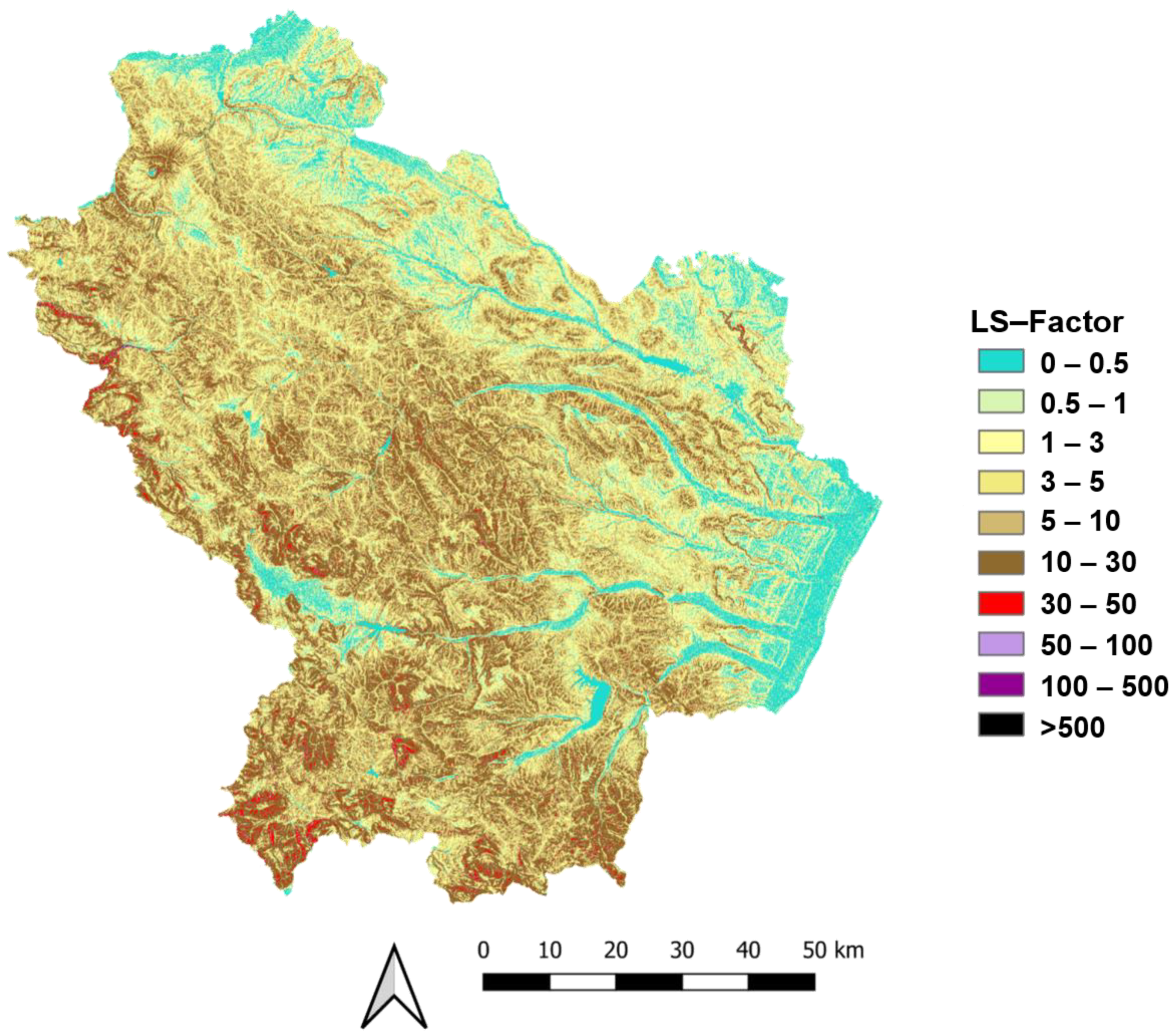
2.2. Slope Length and Slope Steepness Factor LS

The effects of topography and hydrology on erosion rates can be estimated using the non-dimensional factor LS, given by the product of the slope length L and the slope steepness S factors. Areas with steep slopes tend to be more susceptible to erosion than flat areas, and generally, soil erosion increases with increasing slope length.

The extraction of the LS factor is a key issue, since it is the most sensitive parameter of the (R)USLE model in soil loss predictions [35]. The procedure of obtaining the L and S factors was originally done manually [17,20,36], therefore, in the 1980s, their implementation at the watershed scale was unfeasible because their variation was difficult to represent. With the advent of GIS, erosion models started to adopt a spatial representation of erosion processes and features. According to Desmet and Govers [37], in a real two-dimensional situation, overland flow and the resulting soil loss do not really depend on the distance to the divide or upslope border of the field, but on the unit contributing areat, A, i.e., the upslope drainage area per unit of contour length. Thus, several procedures, often based on digital elevation models (DEMs), have been developed in the last 25 years to substitute the slope-length factor with the unit contributing area (see e.g., [36,37,38,39,40]).

In this work, the LS factor was computed in MATLAB using the equation proposed by Moore and Burch [40], Moore and Wilson [36], and Moore et al. [41]:

$$\mathrm{LS}={\left(\frac{As}{a0}\right)}^m\times {\left(\frac{\sin \mathsf{\beta }}{b0}\right)}^n\times \mathrm{Z}$$

(4)

where:

-

A_s is flow path length expressed as the unit contributing area (meters);

-

a0 = 22.13 m and b0 = sin (5.143°) = 0.0896 are, respectively, the length and slope of the standard USLE plot [36];

-

β is slope angle in radian (i.e., β = 3.14* θ/180, where θ is the slope angle in degree);

-

Z is defined as rilling factor, which is used to modify the length slope factor and is developed from the theory of unit stream power, which is usually either 1 or 1.4 (e.g., [9]), and set as 1 in the present work;

-

m and n are physical coefficients generally set as m = 0.4 and n = 1.3 (e.g., [40,42,43,44]).

The required DEM derivatives (specifically the local slope angle (β), the flow direction, and flow accumulation) were computed using TopoToolbox [45], a MATLAB-based software for the topographic analysis of DEMs. Specifically, the following algorithms were used:

-

Slope algorithm, the trigonometrical maximum downward gradient using an 8-connected neighbourhood [45];

-

Flow direction algorithm, the deterministic infinity algorithm (D∞) by Tarboton [39] where the flow direction is partitioned among multiple downslope neighbors determined following the steepest descent and is represented as a continuous quantity between 0 and 2π in direction. Such an algorithm was selected to avoid the widely recognized problem of the single flow direction algorithm (D8) of unrealistically restricting flow pathways to the multiples of 45°, and also to circumvent the unrealistic dispersion introduced by the multiple flow direction algorithm (MFD) [21].

2.3. Cover Management Factor, C

Among the RUSLE elements, the LS and C factors have the greatest impact on modeling soil loss [46], thus, improving the accuracy in the estimate of these factors is essential. The C factor accounts for typology and density of the vegetation cover, since this is a limiting element for erosive processes by reducing the rain impact on soil surface [47].

It represents a dynamic component of the RUSLE model incorporating changes in land cover and management practices [48]. In its original form, the C factor ranged between 0 and 1 and was typically retrieved from in situ surveys. Recently, the advent of a large amount of geospatial data relying mainly on remote sensing platforms, has led to an increasing adoption of simplified forms of the C factor grounded in land cover classifications and vegetation indexes (see e.g., [49]).

The use of land cover maps could introduce errors in highly heterogeneous areas because, generally, they are not able to pick up spatial details of the study area, especially if we want to obtain high resolution soil loss maps. We opted to use a vegetation index to estimate C from Landsat (30 m) data to base our assessment on direct and updated observations. Specifically, we chose the Soil-Adjusted Vegetation Index (SAVI), as proxy for canopy cover, see [50], since it has been proven to be strongly correlated with C factor as compared with other vegetation indices [51]. In particular, the SAVI has been demonstrated to be able to appropriately account for sparsely vegetated areas where, generally, the well-known Normalized Difference Vegetation Index (NDVI) is highly variable [52]. Following [53], we estimated the C factor as:

$$\mathrm{C}=- \mathrm{a}· \mathrm{SAVI}+1$$

(5)

where C is the cover management factor, a = 1.18, and SAVI is obtained by the following equation:

$$\mathrm{SAVI}=\frac{\left[\left(\mathrm{NIR}-\mathrm{RED}\right)·\left(1+\mathrm{L}\right)\right]}{\left(\mathrm{NIR}+\mathrm{RED}+\mathrm{L}\right)}$$

(6)

where L is an adjustment length, usually assumed to be 0.5; NIR and RED are the reflectance values obtained in the near-infrared and red-visible bands, respectively.

The use of vegetation indices to estimate annual variables is not straightforward because of the presence of snow and clouds that limit optical land observations, especially in winter and autumn. Here, we explored the use of a single monthly value (May), because, in this period, all crops in Basilicata are in the growing season, the values of vegetation indices obtained from natural covers are clearly distinguishable from those characteristics of the agricultural ones, and the values effectively separate different phenologies. In addition, this is the most stable month if evaluated on interannual scales [54] and we wanted to avoid average values which could be distorted by land management practices such as crop rotation. The SAVI value in May appears therefore a good candidate to follow the long-term dynamics of land use/land cover.

2.4. Soil-Erodibility Factor, K

The K factor expresses the intrinsic susceptibility of soil to erosion as a function of its properties, such as organic matter content, grain size, permeability, structural integrity, and cohesiveness. In this work over the Basilicata region, we decided to exploit the high-resolution soil erodibility map produced by the JRC of the European Soil Data Centre (ESDAC) (see [55]). This dataset consists of a 500 m resolution K factor map harmonized for the 28 European Union member states. K was calculated using the nomograph of Wischmeier and Smith [17] on about 20,000 points of the Land Use/Cover Area frame Survey (LUCAS) topsoil data [56]. These LUCAS point estimates were then interpolated using a cubist regression model to produce the soil erodibility dataset at 500 m resolution. Then, it was validated against local/regional/national studies found in the literature with very good results. A detailed description of the dataset and the application in Europe is described in [55]. It is freely provided by the JRC for research purposes both with the incorporation or not of the surface stone cover. In this regard, the dataset adopted in the present study does not consider the stoniness and its protective effect against soil erosion.

2.5. Erosion Control Practice Factor, P

The P factor represents the contribution of anti-erosion practices on soil loss, and is a dimensionless parameter ranging between 0 and 1. The cultivation practices that help in reducing erosion contemplated in the RUSLE model are terracing, contouring (cultivation according to topography contour lines), and strip cropping. Among the RUSLE input factors, values for the P factor are considered to be the most uncertain and the effects of support practices on soil erosion reduction by water are difficult to estimate especially for large areas. In this study, to take into consideration the effects of different support practices on soil erosion redcution, the P factor dataset produced by the JRC of the ESDAC was adopted [57]. This P factor was modeled for the European Union taking into consideration contour farming, maintenance of stone walls, and grass margins. It was based on consideration of the latest agro-environmental policies of the Common Agricultural Policy and application of the rules set by the individual member states for contour farming over a certain slope. In addition, the impact of conservation practices such as stone walls and grass margins was modeled using more than 226,000 observations from the LUCAS carried out in 2012 in the European Union. A detailed description of the P factor dataset, its production process, and it application in Europe can be found in the works of Panagos et al. [48,57].

2.6. Procedure for Comparison with Other Local Studies

To be confident in the values of soil loss by water, we implemented a detailed survey of studies that had focused on the study region, starting from a comprehensive review by Borelli et al. [19]. For this purpose, the studies had to contain information on the soil loss values linked to a specific area and a reference period jointly with details on the implemented procedure.

For basin-scale studies, the catchment areas at different orders were downloaded in shape format from the National Environmental Information System Network (SINAnet) of the Italian Institute for Environmental Protection and Research (ISPRA) (additional details are provided in Section 3.2 Dataset). For studies based on sediment deposits in dams, the drainage area that flowed into the dam was identified by combining different catchment orders.

For regional-scale studies with the availability of soil loss maps, the data were acquired and reprojected in UTM WGS84 to be jointly analyzed with our results. In particular, we downloaded the maps of soil loss by water erosion at 100 m resolution available for 2010 and 2016 from the JRC of the ESDAC [55,58]. All the statistics were extracted in QGIS environment.

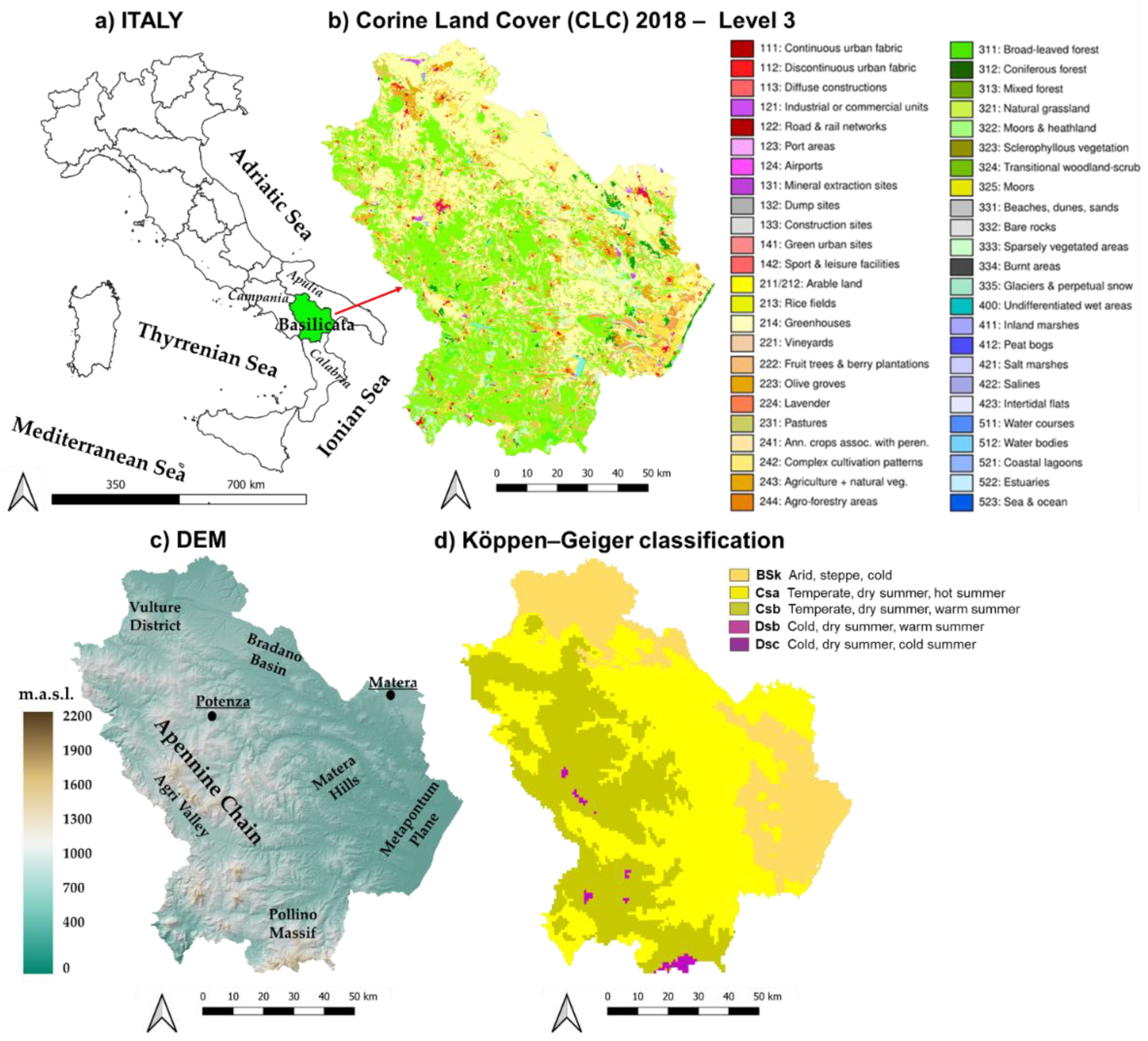
3. Study Area and Dataset

3.1. Study Area

Basilicata is one of 20 regions in Italy (the administrative subdivision corresponding to the European Nomenclature of Territorial Units for Statistics (NUTS2) with a population of about 545,000 inhabitants, according to the Italian National Institute of Statistics (ISTAT) population census of 2020 scattered over a territory of 10,073 km² (Figure 1a).

Land cover appears very heterogeneous (Figure 1b), mostly reflecting orography (Figure 1c). Natural areas characterize high-elevation zones of the Apennine Chain where different forest populations dominate, whose ecological value has led to the establishment of several protected areas, including the Pollino Massif and the Appennino Lucano Val d’Agri Lagonegrese National Park. The north-eastern part of the region bordering Apulia (Bradano Basin) is devoted to agriculture (cereals are the prevalent crop) and, in the volcanogenic basin of the Vulture, vineyards and olive groves give the landscape its distinctive Mediterranean appearance. Arable lands are the main cover also in the central-eastern zone (Matera Hills), characterized by the so-called calanchi, i.e., badlands with bare clay hills strongly affected by erosional processes [59]. The Metaponto Plain, a strip of land overlooking the Ionian Sea, is the core of the specialized agriculture of Basilicata (fruit trees and orchards, see [60]) where salinization phenomena have threaten groundwater quality and soil productivity [61,62]. The peculiarity of Basilicata is the coexistence of the different and, in some ways, contrasting climates it encompasses: the temperate climates (Csa and Csb), the steppic climate (Bsk), and the Mediterranean mountain climates (Dsb and Dsb) characterizing some isolated mountainous areas of the Apennine Chain [63].

Basilicata shows a pronounced vulnerability to land degradation [64] similar to that of most Italian landscapes and Mediterranean countries [65,66,67,68]. This proneness originates from an intrinsic weakness of key environmental parameters: Soils are often thin and with a scarce presence of organic matter [69], while vegetation appears sparse and intermixed with barren areas in many zones [70,71]. In certain areas, climate is the determining factor that amplifies the vulnerability to land degradation [14,72], further exacerbated by the ascertained and increasingly frequent occurrence of extreme events (see e.g., [73,74]).

Lastly, in recent years, human activites have deeply modified landscape patterns, accelerating land degradation phenomena through improper land management [75]; the building of dams, barrages, industrial poles, and tourism facilities [76,77]; and the abandonment of marginal areas [78]. In particular, the cultivation of unsuitable areas fuelled, in some cases, by the Common Agricultural Policy (CAP) (see [79]), since 1992 (MacSharry reform), and the persistent adoption of conventional agricultural techniques providing higher revenues as compared with conservative practices represent the major causes of soil degradation [80]. Alongside this issue, the progressive depopulation recorded in the last two decades has produced widespread phenomena of land abandonment in inner areas, especially in the presence of agriculture founded on low-profitability crops (cereals and traditional olive groves, see, for example, [81]).

3.2. Dataset

All the datasets used in this study were acquired from open-source databases. The topographic parameters (slope, drainage network, and upslope contributing area) were obtained using the 25 m resolution digital elevation model over Europe (EU-DEM, version 1.1) [83], developed by the European Environmental Agency (EEA) through the Copernicus Programme. It is a digital surface model (DSM) derived by fusing Shuttle Radar Topography Mission (SRTM) and Advanced Spaceborne Thermal Emission and Reflection Radiometer (ASTER) Global Digital Elevation Model (GDEM) data through a weighted averaging approach. It should be noted that the selection of the DEM grid size has considerable influence on the soil loss estimation with empirical models. Wu et al. [84] investigated the effect of cell size resolution in describing topographic variability for the estimation of soil loss. According to their study, a 30 m DEM resolution was adequate for soil erosion assessments while, for example, a 100 m should be handled with care due to increased contributing area and decreased slopes. Based on this study, the adopted 25 m DEM should provide an adequate spatial resolution for our purpose.

Regarding the estimate of the rainfall erosivity factor (R), Climate Hazards Group InfraRed Precipitation with Station data (CHIRPS) datasets were collected and analyzed. CHIRPS is a 35+ year (1981 to present) quasi-global (50° S–50° N) daily, pentadal, and monthly rainfall gridded dataset produced at 0.05 × 0.05 degree spatial resolution by incorporating satellite imagery with in situ station data [85]. In this work, we used monthly data to estimate the R factor in the ten-year period just before the date of the soil loss estimations (e.g., for the year 2014 we considered the decade 2004–2013).

Five Landsat images were used to investigate the vegetation cover of the study area and evaluate the C factor and its changes over time. To this aim, the well-known Landsat mission represents the only way to guarantee a diachronic analysis consistent with the rainfall data adopted in this study (CHIRPS time series) with an appropriate spatial detail of 30 m (see, for e.g., [26,86]).

In particular, we used images (188 path and 32 row) from Landsat 8 Operational Land Imager and Thermal Infrared Sensor (OLI/TIRS) (see

Table 1. Bandwidth and spatial resolution of the Landsat 8 OLI/TIRS.

Number of Band	Band Width (µm)	Band Description	Spatial Resolution (m)
1	0.435–0.451	Coastal aerosol	30
2	0.452–0.512	Blue	30
3	0.533–0.590	Green	30
4	0.636–0.673	Red	30
5	0.851–0.879	Near infrared (NIR)	30
6	1.566–1.651	Short wavelength infrared (SWIR) 1	30
7	2.107–2.294	SWIR 2	30
8	0.503–0.676	Panchromatic	15
9	1.363–1.384	Cirrus	30
10	10.60–11.19	Thermal infrared sensor (TIRS)	100
11	11.50–12.51	TIRS 2	100

) and Landsat 5 Thematic Mapper (TM), (see

Table 2. Bandwidth and spatial resolution of the Landsat 5 TM.

Number of Band	Band Width (µm)	Band Description	Spatial Resolution (m)
1	0.45–0.52	Blue	30
2	0.52–0.60	Green	30
3	0.63–0.69	Red	30
4	0.76–0.9	Near infrared (NIR)	30
5	1.55–1.75	Short wavelength infrared (SWIR) 1	30
6	10.40–12.50	Thermal 2	120
7	2.08–2.35	SWIR2	30

) freely downloaded from the United States Geological Survey (USGS) as land-surface reflectance products (Collection 2 Level-2 Science Products (L2SP)):

• 15 May 1994 and 31 May 1994 (composite of the two images for an overall land cloud cover of less than 0.1%);
• 26 May 2004 TM (cloud cover 0%);
• 22 May 2014 OLI (cloud cover 0.24%);
• 9 May 2021 OLI (cloud cover 0.1%).

All the images fall during the spring period, in particular in May, to take into account the presence of many arable crops just before harvesting in order to consider their presence in the erosion estimation.

The persistent cloudiness observed in 1994 forced us to use two images, which were composed in one single image with a cloud cover over less than 0.1% of the overall surface of the Basilicata.

Regarding the K factor and the P factor, the datasets produced by the JRC of the ESDAC are freely obtained upon request; they cover all the European Union with a pixel size of 500 m and 1 km, respectively.

A summary of the main input data used to compute the RUSLE factors is given in

Table 3. Summary of the input data for the RUSLE application.

Input Data	Spatial Resolution	Data Source
Digital elevation model over Europe (EU-DEM)	25 m	Copernicus Land Monitoring Service—EU-DEM, https://www.eea.europa.eu/data-and-maps/data/copernicus-land-monitoring-service-eu-dem, (last accessed, 25 June 2022)
CHIRPS gridded rainfall dataset	0.05°	https://data.chc.ucsb.edu/products/CHIRPS-2.0/, (last accessed, 25 June 2022)
- Landsat 8 OLI/TIRS images - Landsat 5 TM images	30 m	USGS (United States Geological Survey), https://earthexplorer.usgs.gov/, (last accessed, 25 June 2022)
Soil erodibility (K factor) dataset	500 m	Joint Research Centre, European Soil Data Centre (ESDAC), https://esdac.jrc.ec.europa.eu/content/soil-erodibility-k-factor-high-resolution-dataset-europe, (last accessed, 25 June 2022)
Support practices (P factor) dataset	1 km	Joint Research Centre, European Soil Data Centre (ESDAC), https://esdac.jrc.ec.europa.eu/content/support-practices-factor-p-factor-eu, (last accessed, 25 June 2022)
Soil loss by water erosion in Europe (RUSLE 2015)	100 m	Joint Research Centre, European Soil Data Centre (ESDAC), https://esdac.jrc.ec.europa.eu/content/soil-erosion-water-rusle2015, (last accessed, 25 June 2022)
Municipal boundaries of Basilicata	Vector	Italian National Institute of Statistics (ISTAT) https://www.istat.it/it/archivio/222527, (last accessed, 25 June 2022)
,Hydrographic basin boundaries	Vector	The Italian Institute for Environmental Protection and Research (ISPRA), http://www.sinanet.isprambiente.it/it/sia-ispra/download-mais, (last accessed, 25 June 2022)

.

Integration of layers, spatial analysis, and any further calculation were carried out within the GIS environment of QGIS 3.16.16. All datasets were georeferenced in the WGS84 ellipsoid/UTM zone 33 N projection system, resampled to the same pixel size of 30 m.

4. Results

4.1. Rainfall Erosivity Factor (R)

The R factor map was computed for the four decades preceding the years represented in Figure 2.

The spatial distribution of the R values is largely dominated by the orography of the region and partially reflects the distribution of the Koppen–Geiger climate. High values are estimated in the southern most temperate areas on the Apennines that overlook the Thyrrenian Sea, which are also very rainy during summer, whereas the lowest values are estimated for low-level arid areas. The climate variability shown by the different maps in Figure 2 does not alter these spatial clusters, but their characteristic values change in time with maximum values estimated in the twenty-year period 1994–2013 throughout the region. Figure 2e shows an evident interdecadal oscillation, which involves the R distribution over the whole region. During the 1980s, the seasonal distribution of the rainfalls did not indicate significant aggressiveness. Successively, rainfalls became more irregular and abundant over all the region, especially in the wettest areas, with a peak in the decade 2004–2013, which appeared to have the most impact on soil loss. This criticality fades in the decade 2011–2020, which accounts for intermediate climate conditions. The presence of an interdecadal pattern in the R factor is very suggestive, as similar oscillatory behaviours are usually observed in the precipitation intensity and frequency [87] and our approach appears to be able to introduce this information into the estimation of soil loss.

4.2. Slope Length and Slope Steepness Factor LS

Using Equation (4), the LS factor for the Basilicata region was estimated and is represented in Figure 3. The required topographic parameters were extracted from the 25 m resolution DEM using TopoToolbox [45], a MATLAB-based software for the topographic analysis of DEMs.

In

Table 4. Slope length and steepness (LS) factor categories and the corresponding percentage in terms of areal surface in Basilicata (Italy).

LS Factor Categories	Area %
LS ≤ 0.5	10.67
0.5 ≤ LS ≤ 1	7.29
1 ≤ LS ≤ 3	16.60
3 ≤ LS ≤ 5	15.51
5 ≤ LS ≤ 10	27.90
10 ≤ LS ≤ 30	20.40
30 ≤ LS ≤ 50	1.30
50 ≤ LS ≤ 100	0.28
100 ≤ LS ≤ 500	0.04
500 ≤ LS ≤ 5282	0.01

, the LS values are divided into classes and, for each of class, the corresponding percentage of the regional area is reported. The values obtained range between 0 and 5282, with an average value of 7. In half of the region, the values of the LS factor are below 5. Higher values identify places characterized by steeper slopes and increasing unit contributing area(e.g., rills). Since the factor increases more with slope steepness than it does with slope length, the greatest LS values (higher than 30) are mainly located in the western mountainous areas of the Basilicata Apennines, and represent only 1.6% of the region.

4.3. Cover Management Factor, C

In Figure 4, the four maps of C factor are shown, corresponding to the observed years over the period 1994–2021. They indicate roughly a bipartition of Basilicata into two macro-regions: The western region characterized by low C factor values due to a prevalent composition of natural areas with dense canopy cover dominated by large broadleaf forests (see CLC2018 in Figure 1b) and the eastern region, mostly characterized by medium-high C factor values, being predominantly agricultural landscapes mainly composed of arable land (in the Bradano Basin and Matera Hills) and fruit trees (Metaponto Plain). This pattern remains quite stable over time but the magnitude of the C factor values seems to decrease everywhere from 1994 to 2021, with the exception of some areas located in the Agri Valley exhibiting the lowest C factor values in 2014. This picture is coherent with the transformations that occurred in the time frame analyzed in Basilicata, consisting mainly of the agricultural reclamation of large hilly areas in the eastern part of the region and in the notable expansion of forests [88] with the consequent increase in vegetation cover and density implying an increase in the SAVI and a reduction in C factor. Such variations in vegetation density inside agricultural areas are not identifiable in CLC change maps (CHA), where very confined land cover modifications occur during the period 1990–2018.

4.4. Soil-Erodibility Factor K

The K factor values extracted for the Basilicata region from the JRC-ESDAC EU-wide soil erodibility dataset are depicted in Figure 5a.

The chosen dataset does not consider the surface stone cover and its protective effect against soil erosion. This likely produced an overestimation of soil erosion in our final estimate [55].

4.5. Erosion Control Practice Factor, P

The P factor values extracted for the Basilicata region from the JRC-ESDAC dataset are depicted in Figure 5b. Differently from other Italian regions, Basilicata shows limited surfaces where conservative land management systems are adopted.

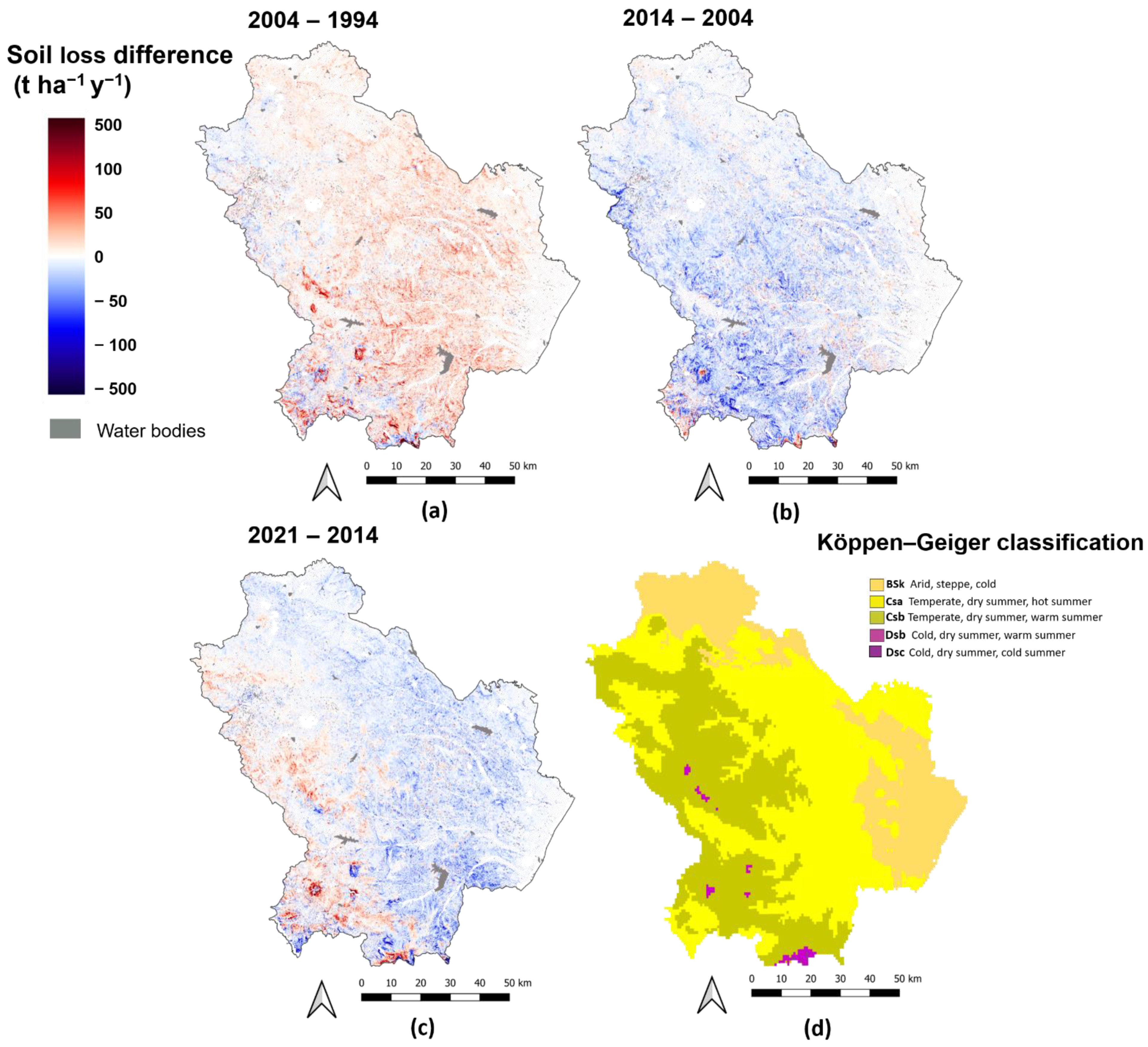
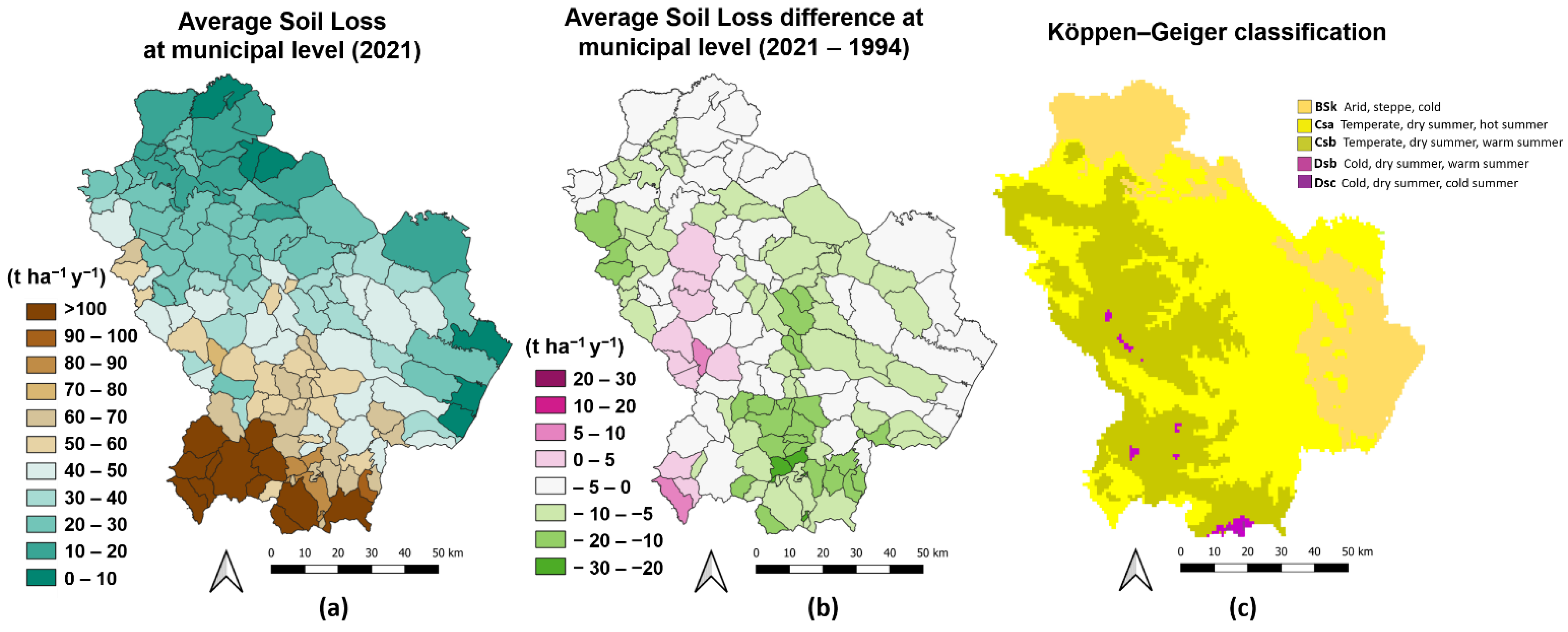
4.6. Soil Loss Maps (1994–2021)

Soil loss rates recorded in Basilicata in the analyzed period are in line with previous works that have focused on single basins or small areas of the same region [33,89]. As shown in Figure 6a,b, the general pattern of soil loss values remains quite similar in the extremes of the time interval analyzed (1994 and 2021). Higher values of soil loss are prevalent in mountain areas within the Lagonegrese area, in the south-western part of the study area, notoriously among the wettest sites of Italy [90]. Sizable scores also characterize the Pollino Massif and, in general, those small areas falling in the Koppen’s Mediterranean mountains climates. Medium-high levels of soil loss are typical in the Matera Hills, in the south-eastern part of Basilicata where there is a large presence of badlands with their peculiar form of differential and selective erosion. Medium-low values prevail in the forests of the western part of the region, while the Bradano Basin and the Metaponto Plain appear to be the less impacted by erosion phenomena due to topographic reasons, being composed of lowlands and areas with gentle slopes. These plain areas overlooking the Ionian Sea are affected by a type of erosion that cannot be assessed with the RUSLE model; coastal erosion affects the entire Ionian coast to a varying extent with soil loss and saline intrusion phenomena [62].

The diachronic picture does not show dramatic changes in soil loss rates between 1994 and 2021 (Figure 6c), with a general, moderate improvement, except for some areas of limited extent within the Lagonegrese area and Agri Valley. These cases are attributable to the different magnitudes of the rainfall erosivity (R factor) recorded in the analyzed years.

Looking at the differences of soil loss computed in the three time intervals (2004–1994, 2014–2004, and 2021–2014, see Figure 7a–c), it is evident that the year 2004 exhibits the worst rates with positive difference found almost everywhere with respect to the year 1994 (Figure 7a). This is due mostly to the high values of the C factor linked to lower canopy coverage and vegetation vigor with respect to the other examined years. The overall conditions of Basilicata improve in 2014 and further in 2021 (Figure 7b,c), with the exception of those areas already highlighted in Figure 6c as the combined effects of lower values of C and R factors. The general increase in cultivated areas, especially in sparsely vegetated and bushy areas, and the expansion of forests are the crucial drivers for the decrease of C factor [88,91], while the rainfall variability produces fluctuations in the R factor values, and then in soil loss estimates, especially in areas falling in the Dsa Köppen-Geiger zones.

This tendency is more clearly highlighted by maps showing the average values of soil loss computed at the municipal level for the year 2021 (Figure 8a) and as soil loss difference for 2021–1994 (Figure 8b). Municipalities falling within the Lagonegrese area and around the Pollino Massif reach the worst values, with rates exceeding 100 t/ha*y. The most alarming fact is that, if we exclude municipalities located in the Bradano Basin and Metaponto Plain, the rest of the study area shows soil erosion rates in 2021 greater than 11 t/ha*y, which is considered by the Organization for Economic Co-operation and Development (OECD) to be the threshold for identifying severe erosion phenomena [92]. This condition persists over time, despite the improvement recorded everywhere between 1994 and 2021 (Figure 8b), with the exception of some municipalities located along the internal areas of the Apennine Chain. This picture appears particularly worrying in light of the well-known limits of the RUSLE model, which only partially accounts for the multiplicity of the erosional processes acting at a local scale (gully erosion, wind erosion, piping, and crop erosion (see [93]), and thus, suggests that the actual soil loss rates could be higher than our estimates. This supports the urgent need to reinforce European policies encouraging environmentally friendly and sustainable agricultural practices, especially through the new CAP 2023–2027. These incentives are mostly critical for Mediterranean regions because they show the highest percentages of agricultural areas affected by severe erosion. Statistics computed at the NUTS2 level include Basilicata in the worst class corresponding to more than 20% of agricultural land impacted by severe forms of erosion [94]. Lastly, climate vulnerability of the Mediterranean Basin is expected to rise in the future with an increase in the rain intensity implying a sure escalation of the erosion issues, especially in the steepest areas [95].

4.7. Comparison with Other Studies

At the local scale, on the basis of the extensive review by Borrelli et al. [19] and our survey, we identified the studies carried out in the Basilicata region that meet the requirements indicated in Section 2.6 (reproducibility of the area and overlapping the period). The comparison of soil estimations by water is quite satisfactory (

Table 5. List of the studies at local level used for the comparison of the RUSLE estimations implemented in the present work.

Local Studies							Present Study
Year	Authors	Title/Reference	Study Area	Period	Method	Soil Loss (t ha−1 yr−1)	Dates	Soil Loss (t ha−1 yr−1)
2012	Fagnano, M., Diodato, N., Alberico, I., Fiorentino, N.	An Overview of Soil Erosion Modeling Compatible with the RUSLE Approach [96]	Sele Basin (part) Lat. 40.37 Lon. 15.25	1973–2007	RUSLE CliFEM	53 ± 43 73 ± 58	1994 2004 1994–2004 average	45.89 46.26 46.07
2015	Aiello, A., Adamo, M., Canora, F.	Remote Sensing and GIS to Assess Soil Erosion with RUSLE3D and USPED at the River Basin Scale in Southern Italy [33]	Bradano Basin Lat. 40.61 Lon 16.42	1991–2011	RUSLE(3D) USPED	31.80 34.35	1994 2004 1994–2004 average	25.72 32.77 29.45
2015	Lazzari, M., Gioia, D., Piccarreta, M., Danese, M., Lanorte, A.	Sediment Yield and Erosion Rate Estimation in the Mountain Catchments of the Camastra Artificial Reservoir (Southern Italy): A Comparison between Different Empirical Methods [89]	Camastra Basin Lat. 40.37 Lon. 15.25	1951–2011	RUSLE(3D) USPED TU index	51.1 16.15 9.95	1994 2004 1994–2004 average	40.64 47.99 44,32
2020	Covelli, C., Cimorelli, L., Pagliuca, D.N., Molino, B., Pianese, D.	Assessment of Erosion in River Basins: A Distributed Model to Estimate the Sediment Production over Watersheds by a 3-Dimensional LS Factor in RUSLE Model [97]	Camastra Basin Lat. 40.37 Lon. 15.25	September 2014–Augest 2018	RUSLE(3D)	71.4	2014 2021	36.83 38.97

), both for values obtained with the RUSLE model and those from other models such as CLiFEM [96] and USPED [33,89]. In particular, data over the Sele basin, even if it belongs only in part to the Basilicata region, are fully in agreement with the estimations obtained by Fagnano et al. [96] with the RUSLE method based on the standard C factor estimation (C table for land use) which were in the range of 53 ± 43 t ha⁻¹ y⁻¹. The comparison over the Bradano basin [33] shows a discrepancy of about 2.5 t ha⁻¹ y⁻¹ with respect to the RUSLE model applied at the local level, whereas it increases to about 5 t ha⁻¹ y⁻¹ with respect to the USPED model. Over the Camastra basin, by evaluating the results of the RUSLE model, our estimations are more in agreement with the study fully covering the period of our dates [89]. By analyzing the data of dam sediment deposition reported in the two studies [89,97] over the Camastra basin obtained from bathymetric surveys (Agency for Development of Irrigation and Land Transformation in Puglia, Lucania, and Irpinia Area), our average 1994–2004 (44.32 t ha⁻¹ y⁻¹) is fully in agreement with the mean sediment deposits of the period 1995–2005 (41.20 t ha⁻¹ y⁻¹, considering a bulk density of 1.9 g cm⁻³ [97]). Among the studies listed in Borrelli et al. [19], the analysis by Capolongo et al. [98] was excluded from the comparison since the erosion estimation values refer to abandoned and remodeled sites obtained from the land cover changes occurred in the period 1955–2002. Such areas are very patchy and difficult to be reproduced without the land cover map of 1955. On the whole, the local scale comparisons show differences of about 11 t ha⁻¹ y⁻¹ and, by excluding one study which considers a period that does not perfectly coincident (the last one in Table 5), our evaluations differ, on average, by about 5 t ha⁻¹ y⁻¹ (minimum 2.5 and maximum 7) with respect to the local estimates obtained with the RUSLE model.

At the regional scale, the comparison with the ESDAC soil loss by water estimations provided very satisfactory results (

Table 6. Mean of percentage differences of soil loss estimation by water between the RUSLE ESDAC map 2016 and the elaborated 2014 map for CLC classes of agricultural areas.

CLC Code	Level 2	Level 3	Difference
211	Arable land	Non-irrigated arable land	−5.27
212	Arable land	Permanently irrigated land	−13.64
221	Permanent crops	Vineyards	−4.15
222	Permanent crops	Fruit trees and berry plantations	−16.26
223	Permanent crops	Olive groves	−7.56
231	Pastures	Pastures	−9.29
241	Heterogeneous agricultural areas	Annual crops associated with permanent crops	−4.16
242	Heterogeneous agricultural areas	Complex cultivation patterns	−7.04
243	Heterogeneous agricultural areas	Land principally occupied by agriculture, with significant areas of natural vegetation	−16.48
244	Heterogeneous agricultural areas	Agro-forestry areas	−16.35

). In particular, for the arable lands, where the standard C table for land use was adopted for ESDAC maps, an average 9.5% difference ((ESDAC2016–2014)/ESDAC2016) was found. A higher difference characterizes permanently irrigated land (~13.5%). Similar dissimilarities are also shown in the other agricultural areas with minimum values for vineyards (4.15%) and annual crops associated with permanent crops (4.16%). The highest differences (~16%) were found for heterogeneous cultivated areas with tree presence and mixed with natural vegetation (e.g., land principally occupied by agriculture, with significant areas of natural vegetation and agro-forestry areas, CLC classes 243 and 244). On average, the difference based on pixel-level comparison is quite good with a percentage difference of about 10%.

5. Discussion

The possibility to adapt the RUSLE model to specific territories and scales and also with limited data availability has spurred numerous authors to test different approaches to derive the basilar factors for its implementation [19,22,23,24]. In this work, we evaluated the usefulness of satellite data (Landsat imagery for C factor and CHIRPS time series for R factor) to estimate soil erosion by water at the regional level. Generally, the C factor based on satellite data is derived by classifying the imagery to obtain land use/land cover at spatial resolution higher than the available land cover maps or with different temporal sampling (e.g., Corine CLC) [26,89,96].

The results obtained from the comparison with the ESDAC maps (mean differences of about 10%) that are based on standard computation of C factor with literature tables for arable lands [58], support the hypothesis of other works for estimating the C factor directly from satellite-based vegetation indices [49,51,53]. One of the relevant points for this choice is the selection of a date representative for the land cover present in the investigated area [33,51]. In our application, May was selected to take into account the presence of very arable crops just before harvesting in order to consider their presence in the erosion estimation.

The use of spatially distributed rainfall data from the CHIRPS time series allowed us to achieve a detailed estimation of R factors also in areas where, generally, pluviometric stations are very scarce, such as mountains, and the standard kriging approaches may not produce representative results [51,89,97]. Even when the stations are present, the availability of the required hourly data is not assured and the monthly data are used with MFI or extended MFI indices [33,97], making the adoption of CHIRPS data easier.

In general, our results overestimated water erosion both at the local and regional scale; higher differences (about 16%) were related to agricultural coverages with a significant presence of natural vegetation areas [49]. This discrepancy was even greater in purely natural areas, such as shrubs and forests, and was in line with the results of Gianinetto et al. [25] who used satellite data for the estimation of the parameter C and found an overestimation of soil loss in forested areas. Apart from the differences among the covers, the homogeneous overestimation we obtained seemed to be more linked to the LS factor. The comparison at the local scale seems to support such an hypothesis (range of overestimation with local application of the RUSLE model 2.5–7.0 t ha⁻¹ y⁻¹) since it highlights that the standard RUSLE model overestimates the gross erosion with respect to the USPED, whereas the RUSLE3D [38] limits such overestimation [33,96].

6. Conclusions

Soil, as a non-renewable resource sustaining life on Earth’s surface, must be protected from natural disturbance factors (wind, rainfall, heatwaves, etc.) and improper tillage practices that can make it unproductive. Erosion is identified as a major threat to soil conservation, especially in Mediterranean regions with intrinsic environmental vulnerabilities and a long history of man-made transformations. Empirical-based modeling approaches, such as the RUSLE model, have achieved the first assessments of the most erosion-sensitive sites over large areas.

In this work, we adopted the RUSLE equation by using various sources of data encompassing European databases, topographic information, and time series of satellite observations to estimate potential soil erosion losses of Basilicata (Southern Italy) over the time span 1994–2021. The spatial distribution of soil loss in Basilicata during this period does not show dramatic changes. Lower values of erosion are generally recorded in 2021, with the exception of some confined areas (Lagonegrese and Agri Valley) showing the reverse pattern. The general greening observed within the region in recent years is a key process to explain the reduction in soil loss amounts. This is due to a combination of the reclamation process fuelled by CAP and started in the late 1990s and early 2000s, which favored durum wheat cultivation in bushy and barren lands, and the rewilding of areas within forests and in their surrounding areas that have contributed to reduce the satellite SAVI value and the C factor (land management). This result puts into evidence the utility of our approach for estimating the role of land use/land cover and related management, which exploits satellite data rather than land cover classifications. Indeed, very local but diffused reclamation processes are generally not picked up by CLC maps, whereas vegetation indices capture them, enabling us to estimate the impact of very local scale interventions on soil loss.

The spatial-temporal trajectories enhanced by the intermediate estimations show slight fluctuations in erosion losses due mostly to rainfall variability. Especially in mountainous areas falling in the Dsa Köppen-Geiger zones, the R factor shows an evident variability with the net local increase phenomena of local rainfall erosivity. These areas are hardly accessible and generally unsuited for agriculture. Here, soil loss rates are mainly expected to be driven by climate variability and changes that can modify rainfall regimes and extreme events. Differently, in the other climate zones that are warmer, drier, and generally characterized by smoother morphologies, land management plays a major role in soil conservation trajectories.

Pixel-based and municipal maps of erosion losses provide options to policymakers for efficiently managing soil issues for prioritization of areas having different pedo-climatic and socioeconomic features. This suggests the establishment of regional (local) strategies to rebalance agricultural and forestry land uses (e.g., favoring arboriculture instead of arable land, promoting afforestation with native species in barren or sparsely vegetated areas, and encouraging agriculture in areas with demographic decline) and to improve the P factor (linked to the adoption of conservative agricultural practices) to match the new ways established by Europe towards environmental sustainability.

The added value of remote sensing data, representing the core of our work, consists in the potential to perform multitemporal analyses of observational data, and thereby to document spatio-temporal patterns for assessing the effects of past and recent policies. The recent validated CHIRPS data, which integrate ground and remote observations, directly provide spatial data, thus, limiting the arbitrariness in the spatial interpolation of data from ground stations performed by single researchers that could lead to different conclusions. The long-term CHIRPS and Landsat datasets, which both assure diachronic (multidecadal) analysis, make estimates more robust and reliable with respect to the use of standard databases, often produced to have global applicability. Remote data provide a dynamic picture of land use/land cover that impacts the spatial/temporal variability of soil loss. In turn, such diachronic assessments provide new insight into the sustainability of land use/land cover in climate changing scenarios at a high level of detail.Starting from this baseline, this research could act as a roadmap for further studies on soil loss estimation in biogeographically complex areas such as Basilicata by using higher temporal, spatial, and spectral resolution datasets (Sentinel-2 and PRISMA) to assist policymakers in soil and land management.

References

1. Panagos, P.; Imeson, A.; Meusburger, K.; Borrelli, P.; Poesen, J.; Alewell, C. Soil Conservation in Europe: Wish or Reality? Land Degrad. Dev. 2016, 27, 1547–1551. [Google Scholar] [CrossRef] [Green Version]
2. Keesstra, S.D.; Bouma, J.; Wallinga, J.; Tittonell, P.; Smith, P.; Cerdà, A.; Montanarella, L.; Quinton, J.N.; Pachepsky, Y.; van der Putten, W.H.; et al. The Significance of Soils and Soil Science towards Realization of the United Nations Sustainable Development Goals. Soil 2016, 2, 111–128. [Google Scholar] [CrossRef] [Green Version]
3. Borrelli, P.; Robinson, D.A.; Panagos, P.; Lugato, E.; Yang, J.E.; Alewell, C.; Wuepper, D.; Montanarella, L.; Ballabio, C. Land Use and Climate Change Impacts on Global Soil Erosion by Water (2015–2070). Proc. Natl. Acad. Sci. USA 2020, 117, 21994–22001. [Google Scholar] [CrossRef] [PubMed]
4. European Commission. Proposal for a Directive of the European Parliament and of the Council Establishing a Framework for the Protection of Soil and Amending Directive 2004/35/EC; European Commission: Brussels, Belgium, 2006.
5. Pimentel, D. Soil Erosion: A Food and Environmental Threat. Environ. Dev. Sustain. 2006, 8, 119–137. [Google Scholar] [CrossRef]
6. Samela, C.; Persiano, S.; Bagli, S.; Luzzi, V.; Mazzoli, P.; Humer, G.; Reithofer, A.; Essenfelder, A.; Amadio, M.; Mysiak, J.; et al. Safer_RAIN: A DEM-Based Hierarchical Filling-&-Spilling Algorithm for Pluvial Flood Hazard Assessment and Mapping across Large Urban Areas. Water 2020, 12, 1514. [Google Scholar] [CrossRef]
7. Eekhout, J.P.C.; de Vente, J. Global Impact of Climate Change on Soil Erosion and Potential for Adaptation through Soil Conservation. Earth-Sci. Rev. 2022, 226, 103921. [Google Scholar] [CrossRef]
8. Borrelli, P.; Robinson, D.A.; Fleischer, L.R.; Lugato, E.; Ballabio, C.; Alewell, C.; Meusburger, K.; Modugno, S.; Schütt, B.; Ferro, V.; et al. An Assessment of the Global Impact of 21st Century Land Use Change on Soil Erosion. Nat. Commun. 2017, 8, 2013. [Google Scholar] [CrossRef] [PubMed] [Green Version]
9. Van der Knijff, J.; Jones, R.; Montanarella, L. Soil Erosion Risk Assessment in Europe; European Soil Bureau, Joint Research Centre EUR: Brussels, Belgium, 2000. [Google Scholar]
10. Panagos, P.; Standardi, G.; Borrelli, P.; Lugato, E.; Montanarella, L.; Bosello, F. Cost of Agricultural Productivity Loss Due to Soil Erosion in the European Union: From Direct Cost Evaluation Approaches to the Use of Macroeconomic Models. Land Degrad. Dev. 2018, 29, 471–484. [Google Scholar] [CrossRef]
11. Terranova, O.; Antronico, L.; Coscarelli, R.; Iaquinta, P. Soil Erosion Risk Scenarios in the Mediterranean Environment Using RUSLE and GIS: An Application Model for Calabria (Southern Italy). Geomorphology 2009, 112, 228–245. [Google Scholar] [CrossRef]
12. Salvati, L.; Gemmiti, R.; Perini, L. Land Degradation in Mediterranean Urban Areas: An Unexplored Link with Planning? Area 2012, 44, 317–325. [Google Scholar] [CrossRef]
13. De Marco, A.; Proietti, C.; Anav, A.; Ciancarella, L.; D’Elia, I.; Fares, S.; Fornasier, M.F.; Fusaro, L.; Gualtieri, M.; Manes, F.; et al. Impacts of Air Pollution on Human and Ecosystem Health, and Implications for the National Emission Ceilings Directive: Insights from Italy. Environ. Int. 2019, 125, 320–333. [Google Scholar] [CrossRef]
14. Lanfredi, M.; Coppola, R.; D’Emilio, M.; Imbrenda, V.; Macchiato, M.; Simoniello, T. A Geostatistics-Assisted Approach to the Deterministic Approximation of Climate Data. Environ. Model. Softw. 2015, 66, 69–77. [Google Scholar] [CrossRef]
15. Orgiazzi, A.; Panagos, P. Soil Biodiversity and Soil Erosion: It Is Time to Get Married. Glob. Ecol. Biogeogr. 2018, 27, 1155–1167. [Google Scholar] [CrossRef]
16. Stefanidis, S.; Alexandridis, V.; Ghosal, K. Assessment of Water-Induced Soil Erosion as a Threat to Natura 2000 Protected Areas in Crete Island, Greece. Sustainability 2022, 14, 2738. [Google Scholar] [CrossRef]
17. Wischmeier, W.H.; Smith, D.D. Predicting Rainfall Erosion Losses—A Guide to Conservation Planning; Department of Agriculture, Science and Education Administration, USDA, Science and Education Administration: Washington, DC, USA, 1978.
18. Renschler, C.S.; Harbor, J. Soil Erosion Assessment Tools from Point to Regional Scales—The Role of Geomorphologists in Land Management Research and Implementation. Geomorphology 2002, 47, 189–209. [Google Scholar] [CrossRef]
19. Borrelli, P.; Alewell, C.; Alvarez, P.; Anache, J.A.A.; Baartman, J.; Ballabio, C.; Bezak, N.; Biddoccu, M.; Cerdà, A.; Chalise, D.; et al. Soil Erosion Modelling: A Global Review and Statistical Analysis. Sci. Total Environ. 2021, 780, 146494. [Google Scholar] [CrossRef] [PubMed]
20. Renard, K.G.; Foster, G.R.; Weesies, G.A.; McCool, D.K.; Yoder, D.C. Predicting Soil Erosion by Water: A Guide to Conservation Planning with the Revised Universal Soil Loss Equation (RUSLE). In Agriculture Handbook; U.S. Government Printing Office: Washington, DC, USA, 1997. [Google Scholar]
21. Garcia Rodriguez, J.L.; Gimenez Suarez, M.C. Methodology for Estimating the Topographic Factor LS of RUSLE3D and USPED Using GIS. Geomorphology 2012, 175, 98–106. [Google Scholar] [CrossRef]
22. Duarte, L.; Cunha, M.; Teodoro, A.C. Comparing Hydric Erosion Soil Loss Models in Rainy Mountainous and Dry Flat Regions in Portugal. Land 2021, 10, 554. [Google Scholar] [CrossRef]
23. Igwe, P.U.; Onuigbo, A.A.; Chinedu, O.C.; Ezeaku, I.I.; Muoneke, M.M. Soil Erosion: A Review of Models and Applications. Int. J. Adv. Eng. Res. Sci. 2017, 4, 237341. [Google Scholar]
24. Alewell, C.; Borrelli, P.; Meusburger, K.; Panagos, P. Using the USLE: Chances, Challenges and Limitations of Soil Erosion Modelling. Int. Soil Water Conserv. Res. 2019, 7, 203–225. [Google Scholar] [CrossRef]
25. Gianinetto, M.; Aiello, M.; Polinelli, F.; Frassy, F.; Rulli, M.C.; Ravazzani, G.; Bocchiola, D.; Chiarelli, D.D.; Soncini, A.; Vezzoli, R. D-RUSLE: A Dynamic Model to Estimate Potential Soil Erosion with Satellite Time Series in the Italian Alps. Eur. J. Remote Sens. 2019, 52, 34–53. [Google Scholar] [CrossRef]
26. Lanorte, A.; Cillis, G.; Calamita, G.; Nolè, G.; Pilogallo, A.; Tucci, B.; De Santis, F. Integrated Approach of RUSLE, GIS and ESA Sentinel-2 Satellite Data for Post-Fire Soil Erosion Assessment in Basilicata Region (Southern Italy). Geomat. Nat. Hazards Risk 2019, 10, 1563–1595. [Google Scholar] [CrossRef]
27. Batista, P.V.G.; Laceby, J.P.; Davies, J.; Carvalho, T.S.; Tassinari, D.; Silva, M.L.N.; Curi, N.; Quinton, J.N. A Framework for Testing Large-Scale Distributed Soil Erosion and Sediment Delivery Models: Dealing with Uncertainty in Models and the Observational Data. Environ. Model. Softw. 2021, 137, 104961. [Google Scholar] [CrossRef]
28. Zhang, H.; Wei, J.; Yang, Q.; Baartman, J.E.M.; Gai, L.; Yang, X.; Li, S.; Yu, J.; Ritsema, C.J.; Geissen, V. An Improved Method for Calculating Slope Length (λ) and the LS Parameters of the Revised Universal Soil Loss Equation for Large Watersheds. Geoderma 2017, 308, 36–45. [Google Scholar] [CrossRef]
29. Renard, K.G.; Foster, G.R.; Weesies, G.A.; Porter, J.P. RUSLE: Revised Universal Soil Loss Equation. J. Soil Water Conserv. 1991, 46, 30–33. [Google Scholar]
30. Fournier, F. Climat et Erosion la Relation Entre L’erosion du sol Par L’eau et Les Precipitations Atmospheriques; Presses Universitaires de France: Paris, France, 1960. [Google Scholar]
31. Arnoldus, H.M.J. An Approximation of the Rainfall Factor in the Universal Soil Loss Equation. In An Approximation of the Rainfall Factor in the Universal Soil Loss Equation; John Wiley and Sons Ltd.: Chichester, UK, 1980; pp. 127–132. [Google Scholar]
32. Ferro, V.; Giordano, G.; Iovino, M. Isoerosivity and Erosion Risk Map for Sicily. Hydrol. Sci. J. 1991, 36, 549–564. [Google Scholar] [CrossRef]