Abstract
Monitoring of the indicator Sustainable Development Goal (SDG) 11.3.1 is important for understanding the coordination between land consumption rate (LCR) and population growth rate (PGR). However, the spatiotemporal indicator SDG 11.3.1 changes at the urban agglomeration (UA) level, and the relationship between LCR and PGR in the prefecture-level cities from different UAs remains unclear. In this study, we monitored the spatiotemporal indicator SDG 11.3.1 in the Yangtze River Economic Belt (YREB) and its three major UAs (i.e., Chengdu–Chongqing (CC), the Middle Reaches of the Yangtze River (MRYR), and the Yangtze River Delta (YRD)) for the periods 2000–2010, 2010–2015, and 2015–2018, using the space–time interaction (STI) method and Pearson’s method. Our major findings were as follows: (1) Compared with the world average of 1.28 for LCRPGR (i.e., ratio of LCR to PGR), except for the LCRPGR of the YRD (2000–2018) and CC (2000–2010), the LCRPGR of CC, the MRYR, and the YREB was lower than 1.28 during 2000–2018. (2) The gaps in both population and built-up area between the YREB and the three UAs did not narrow, but widened. (3) Compared with the LCRPGR in China, except for the LCRPGR of the YRD (2000–2018) and CC (2000–2010), the LCRPGR of the YREB increased from 1.21 to 1.23 between 2000–2010 and 2010–2015, and then decreased to 1.16 in 2015–2018, indicating that the relationship between LCR and PGR in the YREB is relatively stable. (4) A significant positive relationship (p < 0.001) was found between LCR and PGR in CC, the MRYR, the YRD, and the YREB. We conclude that the indicator SDG 11.3.1 is a helpful tool for evaluating land-use efficiency caused by the LCR and PGR at the UA level. Our results provide information support for promoting sustainable and coordinative development between LCR and PGR.
1. Introduction
To address global challenges [1], 193 countries have committed to the 17 Sustainable Development Goals (SDGs), supported by 169 targets [2]. SDG 11 aims to make cities and human settlements inclusive, safe, resilient, and sustainable [3], and the indicator SDG 11.3.1—the ratio (LCRPGR) of the land consumption rate (LCR) to the population growth rate (PGR)—can be used to monitor the land-use efficiency (LUE). Understanding LUE is critical to developing appropriate land policies and population policies, or filling gaps in existing policies.
There are many reports and articles on LCRPGR monitoring at the global [4,5], regional [6,7], national [8], and local [9,10,11,12,13,14,15] levels. As highlighted by Li et al. [6], the procedures used to assess the SDG 11.3.1 indicator differ from city to city. For example, the UN Sustainable Development Goals Report 2017 (UN SDG report 2017) reports that the world average for LCRPGR increased from 1.22 during the period 1990–2000 to 1.28 during the period 2000–2015 [16,17,18]. Estoque et al. [4] showed that the mean LCRPGR decreased by 24%, from 1.34 during the period 1975–2000 to 1.02 during the period 2000–2015. The Big Earth Data in Support of the SDGs (2020) reported that the LCRGR of 433 cities in China increased from 1.33 during 1990–1995 to 2.15 during 2010–2015, and that since 2015 the speed of urban sprawl has slowed down.
The LCRPGR values of sampled cities worldwide in developed countries were 2.1 and 1.9 in 1990–2000 and 2000–2015, respectively. During the same periods, the LCRPGR of 194 stratified sample cities around the world was 1.68 and 1.74, respectively [16]. The LCRPGR values in China were 1.69 and 1.78 during 1990–2000 and 2000–2010, respectively [8]. The SDG 11.3.1 indicator was 0.115 in Poland and −0.054 in Lithuania during 2000–2018, where Poland had an LCR of 0.0462 with a PGR of 0.0132, while Lithuania had an LCR of 0.0067 with a PGR of −0.0067 [19]. From 2007 to 2019, the average LCRPGR in Ethiopia was 1.44, with low land-use efficiency. The average LCR was 6.02, and the average PGR for all cities in Ethiopia was 4.63 [20]. In the four periods of 2000–2005, 2005–2010, 2010–2015, and 2015–2020, the LCRPGR values of Opole were −2.45, −5.88, −5.84, and −4.00, respectively. The highest average growth rates for built-up areas occurred between 3-6 km (11.7%) and more than 6 km (10.4%) from the city center [21]. According to Koroso et al. [22], Addis Ababa’s LCRPGR was 1.02 during the period 2005–2019, whereas the LCRPGR values of the sub-city the city’s total LCRPGR values were 3.16 during the period 2011–2019 and 3.62 during the period 2007–2019. Therefore, there are some discrepancies caused by different regions and geographical scales (i.e., global, regional, national, and local) [23].
The Yangtze River Economic Belt (YREB) has grown rapidly in recent years [24]. Liu et al. [24] showed that the urban expansion in the YREB dropped to 13.39% during the period 2005–2010 and 13.38% during the period 2010–2015. In three urban agglomerations (UAs) (i.e., CC, the MRYR, and the YRD), the increase in urban land in the YRD was higher than in the MRYR and CC from 1995 to 2015, due to the YRD’s natural resources and economic circumstances [24]. In addition, China’s LCRPGR and its spatiotemporal changes from 1990 to 2010 have already been analyzed [8]. Wang et al. [8,25] showed that the mean LCRPGR in China increased from 1.69 during the period 1990–2000 to 1.78 during the period 2000–2010 [8,25].
However, spatiotemporal LCRPGR changes, LUE, and the relationship between LCR and PGR at the UA level are either not completely studied, or are missing; lacking this information and knowledge hinders our ability to build policies towards sustainable development for the future at the UA level [26,27].
In this study, we employed the indicator SDG 11.3.1, the space–time interaction (STI) method, and Pearson’s method of LCRPGR to quantify the spatiotemporal LCRPGR changes, LUE, and the relationship between LCR and PGR across the YREB and its three major UAs (i.e., Chengdu–Chongqing (CC), the Middle Reaches of the Yangtze River (MRYR), and the Yangtze River Delta (YRD)) for 2000–2015 and its three sub-periods (i.e., 2000–2010, 2010–2015, and 2015–2018). This work also can help fill the gap in SDG indicator 11.3.1 at the UA level. Therefore, the specific objectives of this study are to (1) illustrate the tends of built-up expansion and population growth in CC, the MRYR, the YRD, and the YREB during 2000–2018; (2) explore the spatiotemporal LCRPGR changes in CC, the MRYR, the YRD, and the YREB for three periods (2000–2010, 2010–2015, and 2015–2018); and (3) quantify the relationship between LCR and PGR in the prefecture-level cities. Our results provide information support for promoting sustainable and coordinative development between LCR and PGR, and also have important implications for spatial projections of future urban expansion.
2. Materials and Methods
2.1. Study Site
The YREB encompasses two municipalities and nine provinces (Figure 1). It covers roughly 21.3% of the total Chinese area, and has a population of almost 600 million, contributing more than 44.3% of China’s GDP. The YREB is one of the fastest-growing regions [28,29], and consists of three major UAs: the Yangtze River Delta (YRD), the Middle Reaches of the Yangtze River (MRYR), and Chengdu–Chongqing (CC). Rapid urbanization and extensive economic activities in the YREB can reflect the various characteristics and patterns of LUE [24,30].
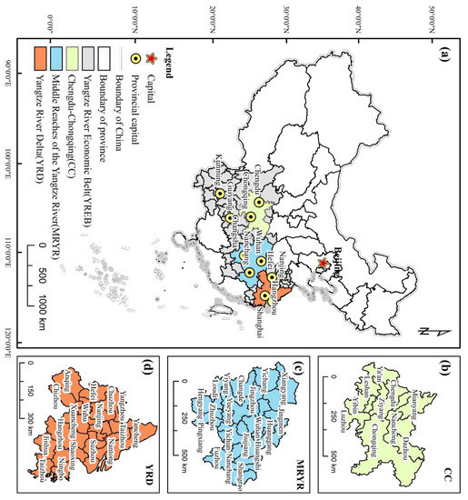
Figure 1.
The location and boundaries of (a) the YREB, (b) CC, (c) the MRYR, and (d) the YRD.
2.2. Data Used
Three datasets, including raster maps of built-up area and population data, and shapefile maps of boundaries of YREB data, were used in this study. The land use/land cover (LULC) type of “Built-up land” in China’s Land-Use/Cover Datasets (CLUDs) (spatial resolution: 100 m) for 2000, 2010, 2015, and 2018 was downloaded from the website of the Data Centre for Resources and Environmental Sciences. Population data (spatial resolution: 100 m) for 2000, 2010, 2015, and 2018 were acquired from the WorldPop Project at https://www.worldpop.org/geodata/listing?id=16 (accessed on 7 May 2022). Boundaries of the YREB were taken from the National Fundamental Geography Information System webpage http://www.ngcc.cn/ngcc/ (accessed on 11 May 2022).
2.3. Applied Method
2.3.1. The Flowchart
Figure 2 presents the flowchart of this study. Firstly, we calculated the LCRPGR and analyzed the spatial patterns of its change over time in the prefecture-level cities and across the UAs in the YREB for 2000–2010, 2010–2015, and 2015–2018. We then used the STI method to understand the spatiotemporal dynamics of LCRPGR. Moreover, we determined the statistical relationship between LCR and PGR using Pearson’s correlation analysis. Finally, according to the results and policy, we concluded that the LUE should be monitored from the perspective of PGR versus LCR to achieve the sustainable development of the UAs.
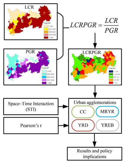
Figure 2.
This study’s flowchart. CC: Chengdu–Chongqing; MRYR: Middle Reaches of the Yangtze River; YRD: Yangtze River Delta; YREB: Yangtze River Economic Belt.
2.3.2. Estimating the Indicator SDG 11.3.1
SDG 11.3.1 is primarily used to quantify the LUE as a consequence of spatially consumed land against the rate at which their populations grow [31,32]. The upper bound was defined as the LCRPGR value located close to the value of the top 2.5th percentile; the lower bound was defined as the LCRPGR value located close to the value of the bottom 2.5th percentile. We then classified the LCRPGR into five categories: LCRPGR ≤ −1.0, −1.0 < LCRPGR ≤ 0.0, 0.0 < LCRPGR ≤ 1.0, 1.0 < LCRPGR ≤ 2.0, and LCRPGR > 2.0 [4,8].
where Urbt and Urbt+n are the total areal extent of land consumed at the given spatial unit (e.g., prefecture-level city) for the initial year (t, 2000, then 2010, 2015) and final year (t + n, 2010, then 2015, 2018), respectively; Popt and Popt+n represent the total population at the given the corresponding spatial unit for the initial year (t) and final year (t + n), respectively; is the number of years between t and t + n; and ln refers to a natural logarithm.
Urb was derived from urban construction land based on the practical definition proposed by Song et al. [28] of the built-up boundary that maintains the core area of the city, and we removed independent pixels (within 5 pixels), small areas at the edge of the city, and satellite cities. This paper selects a multiphase land-use dataset, in which construction land is divided into urban construction land and rural residential land. Taking urban construction land as the scope of Urb, the Urb of the multiphase in-study area was extracted. Then, the extracted Urb was divided into 1 km × 1 km grids, and the percentage of the Urb was calculated in each grid in the YREB from 2000 to 2018.
2.3.3. Deriving Land-Use Efficiency
Land-use efficiency (LUE), defined as the rate of change in LCRPGR between the first time period (P1) and the second time period (P2), was derived using the following formula:
A positive value indicates that land-use efficiency decreases over time, while a negative value indicates an increase in LUE. We classified the LUE into seven categories: high increase (≤−100%), medium increase (−100% to −50%), low increase (−50% to 0%), no change (0%), low decrease (0% to 50%), medium decrease (50% to 100%), and high decrease (>100%) [4].
2.3.4. Spatiotemporal Analysis
We used the space–time interaction (STI) method given by Legendre et al. [33] to understand the spatial and temporal dynamics of LCRPGR. This method tests for space–time interactions in repeated data, where there are no replications at the level of individual sampling units. In STI, variables of time and space are coded using principal coordinates of neighbor matrices in a two-way analysis of variance (ANOVA) model [34]. The STI’s significant results (p < 0.05) show that LCRPGR’s spatial distribution has changed over time. In this study, we used the R package adespatial (version 0.3–8) to process STI, setting each STI test at 999 permutations [33,35].
2.3.5. Statistical Analysis
We used a correlation analysis (i.e., Pearson’s r) to examine the statistical relationship between LCR and PGR during the period 2000–2018 in CC, the MRYR, the YRD, and the YREB.
3. Results
3.1. Trends of Built-Up Expansion and Population Growth
On average, the YREB’s population has been increasing at a rate of 3.05 million people/year, while the YREB’s built-up area has been expanding at a speed of 928.83 km2/year. Specifically, the YREB’s population increased 2.1-fold from 54.44 million in 2000 to 112.38 million in 2018 (Figure 3a), and its built-up area increased 2.7-fold from 10,436.74 km2 in 2000 to 28,084.58 km2 in 2018 (Figure 3b).
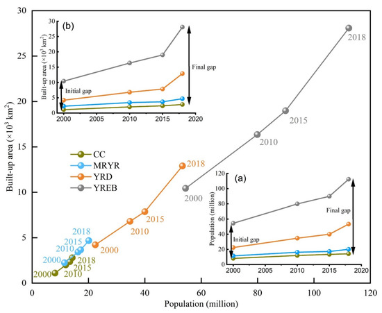
Figure 3.
Relationship between population and built-up area at the UA level: (a) Trends of population growth across the four UAs (i.e., CC, MRYR, YRD, and YREB) from 2000 to 2018. (b) Trends of built-up expansion across the four major UAs from 2000 to 2018.
CC’s population increased 1.8-fold from 8.12 million in 2000 to 14.26 million in 2018, and its built-up area increased 2.5-fold from 1101.66 km2 in 2000 to 2788.74 km2 in 2018. The MRYR’s population increased 1.8-fold from 11.48 million in 2000 to 20.12 million in 2018, and its built-up area increased 2.1-fold from 2242.76 km2 in 2000 to 4685.7 km2 in 2018. The YRD’s population increased 2.4-fold from 22.45 million in 2000 to 53.36 million in 2018, and its built-up has area increased 3.1-fold from 4218.09 km2 in 2000 to 12,899.52 km2 in 2018 (Figure 3).
In three UAs (i.e., CC, the MRYR, and the YRD), the YRD had the highest proportion of the YREB’s population and built-up area during 2000–2018 (Figure 3a,b). Both the population and the built-up area of the MRYR and CC have increased over the years. Regardless of population or built-up area, the percentage share of the YRD has always been the highest. During 2000–2018, the gaps in both population and built-up area between YREB and the three UAs did not narrow, but widened (Figure 3a,b).
3.2. Spatiotemporal LCRPGR Changes
At the UA level, CC had the highest land-use efficiency in the three periods, followed by the MRYR, YRD, and YREB (Table 1). A major difference was that the land-use efficiency of the YRD decreased over the three periods, whereas that of the MRYR and YREB first decreased and then increased (Table 1).

Table 1.
LCRPGR and LUE at the UA level.
Moreover, in the prefecture-level cities, the LCRPGR increased (LCRPGR > 0) in 16 (100%), 13 (81%), and 11(69%) of the 16 prefecture-level cities across CC in 2000–2010, 2010–2015, and 2015–2018, respectively (Figure 4 and Table 2). Specifically, the MRYR, YRD and YREB had the highest proportions in 25 ± 2 (89 ± 8%) of 28 prefecture-level cities, 24 ± 1 (97 ± 3%) of 25 prefecture-level cities, and 113 ± 7 (83 ± 5%) of 126 prefecture-level cities with increasing LCRPGR values, respectively (Figure 4 and Table 2).
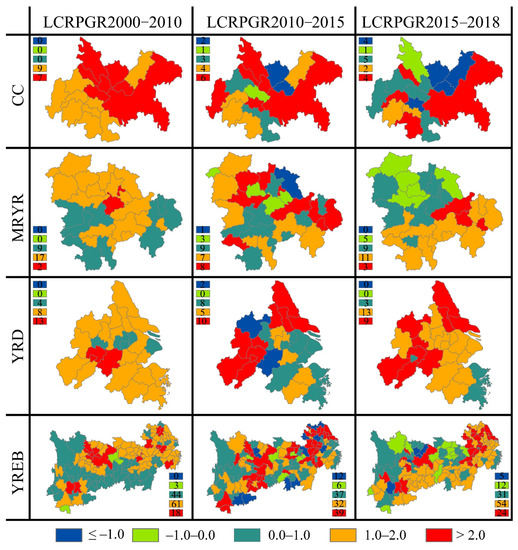
Figure 4.
Spatial patterns of the LCRPGR values across CC, the MRYR, the YRD, and the YREB in 2000–2010, 2010–2015, and 2015–2018. A positive value for LCRPGR indicates an increase in built-up area and population over the period, while a negative value indicates a decrease. The numbers in the legend represent the count of prefecture-level cities of each classification.
Table 2.
Statistics on the number prefecture-level cities of LCRPGR < 0 and LCRPGR > 0 for 2000–2010, 2010–2015, and 2015–2018 in CC, the MRYR, the YRD, and the YREB.
In Figure 5, the spatiotemporal dynamics of the LCRPGR in all prefecture-level cities are shown. For CC (Figure 5a), an obvious initial decrease and subsequent increase was observed from 2000 to 2018. In contrast, a clear initial increase and subsequent decrease was observed across the MRYR (Figure 5b) during the same periods. For the YRD (Figure 5c) and YREB (Figure 5d), LCRPGR showed a weak growth trend and tended to stabilize over time, respectively. Results from the STI analysis (p < 0.05) indicate that this stabilization trend only happened in a few specific prefecture-level cities (Figure 5d). In reality, the spatial patterns of LCRPGR were affected by not only the spatial heterogeneity in the YREB (p < 0.05), but also the conditions of natural resources and the economic basis.
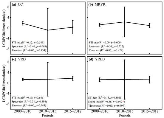
Figure 5.
STI test results for LCRPGR across prefecture-level cities in (a) CC, (b) the MRYR, (c) the YRD, and (d) the YREB over the entire study period (2000–2018) (mean ± SD across all prefecture-level cities). ⁎ Significance level of 0.05.
Overall, the spatiotemporal dynamics of the LCRPGR showed that the selected UAs experienced a fluctuation trend. Only trends in the YRD increased weakly, while trends in the YREB tended to stabilize from 2000 to 2018.
3.3. Relationship between LCR and PGR
A significant positive relationship (p < 0.001) was found between LCR and PGR in CC, the MRYR, the YRD, and the YREB (Figure 6). In the prefecture-level cities, LCR and PGR were also positively and significantly correlated over the entire study period (2000–2018) in the four UAs, namely, CC (N = 48, Pearson’s r = 0.425, p < 0.001), the MRYR (N = 84, Pearson’s r = 0.90, p < 0.001), the YRD (N = 75, Pearson’s r = 0.85, p < 0.001), and the YREB (N = 378, Pearson’s r = 0.83, p < 0.001) (Figure 6).
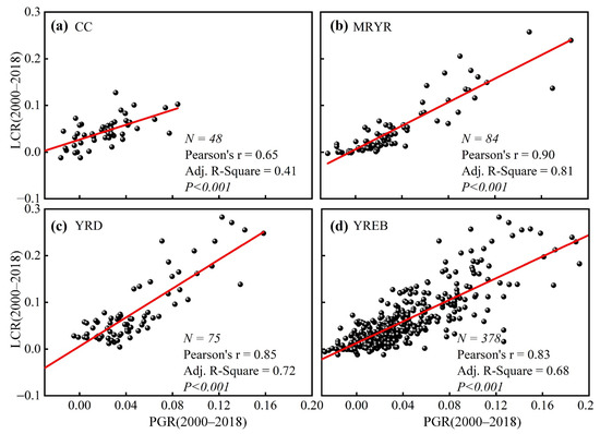
Figure 6.
Scatterplots describing the relationships between LCR and PGR across (a) CC, (b) the MRYR, (c) the YRD, and (d) the YREB during 2000–2018. Each point represents a prefecture-level city.
4. Discussion
According to UN-Habitat reports, cities are expanding spatially at a faster rate than population growth, which can cause problems and have an impact on city-related disasters, climate change, urban planning, and policies [32].
The indicator SDG 11.3.1 was designed to monitor LUE as urbanization threatens urban sustainable development. This study uses CLUDs data to extract information on built-up land, and combines population data to calculate and monitor the LCRPGR of the YREB and its three major UAs in China.
The world average LCRPGR value given by the UN SDG report 2017 for the period 2000–2015 was 1.28 [6,18]. Compared with the world average of 1.28 for LCRPGR, except for the LCRPGR of the YRD (2000–2018) and CC (2000–2010), the LCRPGR of CC, the MRYR, and the YREB was lower than 1.28 throughout the entire study period (2000–2018) (Table 1), indicating that LCRPGR in CC, the MRYR, and the YREB was lower than the world average.
The Big Earth Data in Support of the SDGs (2020) reported that the LCRGR of 433 cities in China increased from 1.33 during 1990–1995 to 2.15 during 2010–2015, and that since 2015 the rate of urban expansion has slowed down. Compared with the LCRPGR in China, except for the LCRPGR of the YRD (2000–2018) and CC (2000–2010), the LCRPGR of the YREB increased from 1.21 during the period 2000–2010 to 1.23 during the period 2010–2015, and then decreased to 1.16 during the period 2015–2018 (Table 1), indicating that the relationship between LCR and PGR in the YREB is relatively stable, but it belongs to the urban land expansion type. Unlike Opole, Ethiopia, and other urban agglomerations in China [20,21], most cities in the YREB have a positive LCRPGR, while CC had a negative LCRPGR during 2010–2015 due to negative population growth in surrounding small cities. Chengdu and Chongqing, as economically developed cities in the southwestern region, have obvious core–periphery effects on the surrounding small cities, leading to the phenomenon of population loss. The core–periphery effects are reflected in the migration of the central and western population to the eastern region in China, or the strong attraction to the population of surrounding cities, suburbs, and rural settlements [25]. The LCRPGR values of the YREB were 1.21, 1.23, and 1.16 in 2000–2010, 2010–2015, and 2015–2018, respectively, which were lower than the LCRPGR values of 2.1 and 1.9 in 1990–2000 and 2000–2015 for sampled cities in developed countries, respectively [16]. The value of LCRPGR in the MRYR during the period 2010–2015, and in the YRD during the period 2015–2018, slightly outperformed the global stratified sample city average LCRPFR in 1990–2000 and 2000–2015 (1.68 and 1.74, respectively), and surpassed China’s LCRPGR in 1990–2000 and 2000–2010 (1.69 and 1.78, respectively).
The UAs that changed most dramatically were CC and the MRYR, which decreased from 1.77 during the period 2000–2010 to −0.82 during the period 2010–2015, and then to 0.31 during the period 2015–2018 (Table 1). By contrast, the MRYR and CC increased from 1.23 during the period 2000–2010 to 2.35 during the period 2010–2015, and then to 0.92 during the period 2015–2018, indicating that the LCR and PGR in CC and the MRYR underwent significant changes. This could be due to two reasons: Firstly, the average LCRPGR values given by the UN SDG report 2017 and the Big Earth Data in SDGs (2020) were calculated based on a different data source as those of this paper. Secondly, UAs of different sizes and different urban expansion types are used to calculate the average LCRPGR within a geographical area, which mainly shows the average level of LUE, and does not pay attention to cities with severe urban land growth or severe urban population growth phenomena.
Theoretically, a reasonable LCRPGR value should be equal to or close to 1 [36], indicating a balance between urban land-use consumption and population growth in UAs. This study shows that there were two types of change trends during the measurement periods 2000–2010, 2010–2015, and 2015–2018 (Table 1): One is that the LCRPGR value for the MRYR and YREB for the period 2015–2018 is closer to the ideal value of 1 than the values for the periods 2000–2010 and 2010–2015, meaning that the urban land-use efficiency was improved in the MRYR and YREB. The second is that the LCRPGR value in CC and the YRD for the period 2000–2010 is closer to the ideal value of 1 than the values for the periods 2010–2015 and 2015–2018, which means that the urban land-use efficiency declined in CC and the YRD. Therefore, CC and the YRD are facing the problem of inefficient use of urban land, either with relatively larger or smaller urban land consumption compared with the PGR [7]. Due to differences in factors such as socioeconomics, regional locations, and policy orientations, there are differences in the expansion intensity of different cities. For example, the growth of the built-up area in CC is mainly reflected in the provincial capital cities. Because the provincial capital cities have a strong attraction to the whole province, the built-up area of the provincial capital cities has grown rapidly. In terms of policy, the dual land system has led to the formation of two markets—for agricultural land and non-agricultural land—in China’s land market. The low cost of land acquisition and rapid industrial development have transformed a large number of agricultural land markets into non-agricultural land markets, driving the growth of urban land consumption rates. Different land policies in different cities also lead to differences in land-use efficiency.
It is worth noting that our calculated results have many outliers of LCRPGR. These outliers of LCRPGR are generated mostly by small changes in urban population growth over time [6]. If these outliers of LCRPGR are used to evaluate the LUE, it will inevitably reduce the reliability of the results [6]. Thus, relevant scholars need to revise the SDG 11.3.1 indicator to conceive a more comprehensive one [4].
On the scale of UAs, a significant positive relationship (p < 0.001) was found between LCR and PGR (Figure 6), which is inconsistent with the findings of Estoque et al. [4], who found a significant positive relationship between LCR and PGR in only some regions [4]. One possible reason for this difference might be related to land-use policies. China’s land-centered expansion of built-up areas is influenced by regulatory land control from land governance and land-use planning [24]. Therefore, the land-use policies of the country’s establishment can guide land consumption for the local government, and can provide instruction to properly arrange newly increased urban land to maximize the benefits of regional integration [24]. This finding might have important implications in spatial simulation and spatial prediction models of future urban expansion [4], especially at the UA level.
There are several papers in the literature on LCRPGR monitoring at the global [4,5], regional [6,7], national [8], and local [9,10,11,12,13,14,15] levels. As highlighted by Li et al. [6], the procedures used to assess the indicator SDG 11.3.1 differ from city to city. Therefore, it is very difficult to compare their results. We suggest that the administrative boundaries of the LCR and PGR calculations are the same [4], and that those data used should be highly spatiotemporally consistent, so as to ensure that the results of the monitored land-use efficiency are statistically comparable with one another.
5. Conclusions
We monitored the LCRPGR in the YREB and its three major UAs (i.e., CC, the MRYR, and the YRD) for 2000–2018 and its three sub-periods (i.e., 2000–2010, 2010–2015, and 2015–2018), mapping spatiotemporal LCRPGR changes and relationships between LCR and PGR in the prefecture-level cities using the indicator SDG 11.3.1, STI, and Pearson’s method, and analyzing the spatial pattern of LCRPGR changes over time at the UA level. Three major findings are supported: (1) On average, the YREB’s population has been growing at a rate of 3.05 million people/year, and the YREB’s built-up area has been expanding at a rate of 928.83 km2/year. (2) The gaps in both population and built-up area between the YREB and the three UAs has not narrowed, but widened. (3) At the UA level, the spatial and temporal dynamics of the LCRPGR indicate that the majority of the selected UAs showed a fluctuation trend. Only trends in the YRD increased weakly, while trends in the YREB tended to stabilize from 2000 to 2018. (4) A significant positive relationship (p < 0.001) was found between LCR and PGR in CC, the MRYR, the YRD, and the YREB. Our findings can help to monitor LUE in UAs, and to provide a case study in monitoring the SDG 11.3.1 for UAs.
Author Contributions
Conceptualization, B.L.; Formal Analysis, Y.W. and B.L.; Funding Acquisition, B.L. and L.X.; Methodology, B.L.; Resources, Y.W. and B.L.; Supervision, B.L.; Visualization, Y.W. and B.L.; Writing—Original Draft, Y.W. and B.L.; Writing—Review and Editing, Y.W. and B.L. All authors have read and agreed to the published version of the manuscript.
Funding
This work was supported by the National Natural Science Foundation of China (Grant No. 42101259), the China Postdoctoral Science Foundation (Grant No. 2021M702508), the Young Talent Fund of Association for Science and Technology in Shaanxi, China (Grant No. XXJS202234), the Key Laboratory of Spatial-temporal Big Data Analysis and Application of Natural Resources in Megacities, MNR (Grant No. KFKT-2022-08), the Fundamental Research Funds for the Central Universities (Grant No. 2042021kf0006), and the Open Fund of the National Engineering Research Center for Geographic Information Systems, China University of Geosciences, Wuhan 430074, China (Grant No. 2021KFJJ03).
Institutional Review Board Statement
Not applicable.
Informed Consent Statement
Not applicable.
Data Availability Statement
Land-use/land-cover (LULC) datasets were downloaded from the Data Centre for Resources and Environmental Sciences (RESDC) webpage http://www.resdc.cn/data.asp x?DATAID = 99 (accessed on 5 May 2022). Population data were acquired from WorldPop at https://www.worldpop.org/geodata/listing?id=16 (accessed on 7 May 2022). Boundaries of the YREB were taken from the National Fundamental Geography Information System webpage http://www.ngcc.cn/ngcc/ (accessed on 11 May 2022).
Acknowledgments
We are grateful to the anonymous reviewers for their valuable comments and suggestions to improve this study.
Conflicts of Interest
The authors declare no conflict of interest.
References
- Parnell, S. Defining a Global Urban Development Agenda. World Dev. 2016, 78, 529–540. [Google Scholar] [CrossRef]
- UN. World Urbanization Prospects: The 2018 Revision; Department of International Economic and Social Affairs, United Nations: New York, NY, USA, 2018. [Google Scholar]
- UN. Twitter, UN Global Pulse Announce Data Partnership. 2016. Available online: https//www.un.org/sustainabledevelopment/cities/ (accessed on 6 May 2022).
- Estoque, R.C.; Ooba, M.; Togawa, T.; Hijioka, Y.; Murayama, Y. Monitoring Global Land-Use Efficiency in the Context of the UN 2030 Agenda for Sustainable Development. Habitat Int. 2021, 115, 102403. [Google Scholar] [CrossRef]
- Melchiorri, M.; Pesaresi, M.; Florczyk, A.J.; Corbane, C.; Kemper, T. Principles and Applications of the Global Human Settlement Layer as Baseline for the Land Use Efficiency Indicator—SDG 11.3.1. ISPRS Int. J. Geo-Inf. 2019, 8, 96. [Google Scholar] [CrossRef] [Green Version]
- Li, C.; Cai, G.; Du, M. Big Data Supported the Identification of Urban Land Efficiency in Eurasia by Indicator SDG 11.3.1. ISPRS Int. J. Geo-Inf. 2021, 10, 64. [Google Scholar] [CrossRef]
- Li, C.; Cai, G.; Sun, Z. Urban Land-Use Efficiency Analysis by Integrating LCRPGR and Additional Indicators. Sustainability 2021, 13, 13518. [Google Scholar] [CrossRef]
- Wang, Y.; Huang, C.; Feng, Y.; Zhao, M.; Gu, J. Using Earth Observation for Monitoring SDG 11.3.1-Ratio of Land Consumption Rate to Population Growth Rate in Mainland China. Remote Sens. 2020, 12, 357. [Google Scholar] [CrossRef] [Green Version]
- Ghazaryan, G.; Rienow, A.; Oldenburg, C.; Thonfeld, F.; Trampnau, B.; Sticksel, S.; Jürgens, C. Monitoring of Urban Sprawl and Densification Processes in Western Germany in the Light of SDG Indicator 11.3.1 Based on an Automated Retrospective Classification Approach. Remote Sens. 2021, 13, 1694. [Google Scholar] [CrossRef]
- Cai, G.; Zhang, J.; Du, M.; Li, C.; Peng, S. Identification of Urban Land Use Efficiency by Indicator-SDG 11.3.1. PLoS ONE 2020, 15, e0244318. [Google Scholar] [CrossRef]
- Mudau, N.; Mwaniki, D.; Tsoeleng, L.; Mashalane, M.; Beguy, D.; Ndugwa, R. Assessment of SDG Indicator 11.3.1 and Urban Growth Trends of Major and Small Cities in South Africa. Sustainability 2020, 12, 63. [Google Scholar] [CrossRef]
- Schiavina, M.; Melchiorri, M.; Corbane, C.; Florczyk, A.; Freire, S.; Pesaresi, M.; Kemper, T. Multi-Scale Estimation of Land Use Efficiency (SDG 11.3.1) across 25 Years Using Global Open and Free Data. Sustainability 2019, 11, 5674. [Google Scholar] [CrossRef] [Green Version]
- Jalilov, S.M.; Chen, Y.; Quang, N.H.; Nguyen, M.N.; Leighton, B.; Paget, M.; Lazarow, N. Estimation of Urban Land-Use Efficiency for Sustainable Development by Integrating over 30-Year Landsat Imagery with Population Data: A Case Study of Ha Long, Vietnam. Sustainability 2021, 13, 8848. [Google Scholar] [CrossRef]
- Gilani, H.; Ahmad, S.; Qazi, W.A.; Abubakar, S.M.; Khalid, M. Monitoring of Urban Landscape Ecology Dynamics of Islamabad Capital Territory (ICT), Pakistan, over Four Decades (1976-2016). Land 2020, 9, 123. [Google Scholar] [CrossRef] [Green Version]
- Philip, E. Coupling Sustainable Development Goal 11.3.1 with Current Planning Tools: City of Hamilton, Canada. Hydrol. Sci. J. 2021, 66, 1124–1131. [Google Scholar] [CrossRef]
- The Sustainable Development Goals Report 2016; United Nations: New York, NY, USA, 2016.
- SDG Indicator Training Module. Land Use Efficiency; 11.3.1; UN-Habitat: Nairobi, Kenya, 2018.
- The Sustainable Development Goals Report 2017; United Nations: New York, NY, USA, 2017.
- Calka, B.; Orych, A.; Bielecka, E.; Mozuriunaite, S. The Ratio of the Land Consumption Rate to the Population Growth Rate: A Framework for the Achievement of the Spatiotemporal Pattern in Poland and Lithuania. Remote Sens. 2022, 14, 1074. [Google Scholar] [CrossRef]
- Koroso, N.H.; Lengoiboni, M.; Zevenbergen, J.A. Urbanization and Urban Land Use Efficiency: Evidence from Regional and Addis Ababa Satellite Cities, Ethiopia. Habitat Int. 2021, 117, 102437. [Google Scholar] [CrossRef]
- Wiatkowska, B.; Słodczyk, J.; Stokowska, A. Spatial-Temporal Land Use and Land Cover Changes in Urban Areas Using Remote Sensing Images and Gis Analysis: The Case Study of Opole, Poland. Geosciences 2021, 11, 312. [Google Scholar] [CrossRef]
- Koroso, N.H.; Zevenbergen, J.A.; Lengoiboni, M. Urban Land Use Efficiency in Ethiopia: An Assessment of Urban Land Use Sustainability in Addis Ababa. Land Use Policy 2020, 99, 105081. [Google Scholar] [CrossRef]
- Guo, H.; Liang, D.; Chen, F.; Shirazi, Z. Innovative Approaches to the Sustainable Development Goals Using Big Earth Data. Big Earth Data 2021, 5, 263–276. [Google Scholar] [CrossRef]
- Liu, Y.; Zhang, X.; Kong, X.; Wang, R.; Chen, L. Identifying the Relationship between Urban Land Expansion and Human Activities in the Yangtze River Economic Belt, China. Appl. Geogr. 2018, 94, 163–177. [Google Scholar] [CrossRef]
- Wang, Y.; Huang, C.; Zhao, M.; Hou, J.; Zhang, Y.; Gu, J. Mapping the Population Density in Mainland China Using NPP/VIIRS and Points-Of-Interest Data Based on a Random Forests Model. Remote Sens. 2020, 12, 3645. [Google Scholar] [CrossRef]
- Zhang, Z.; Hu, Z.; Zhong, F.; Cheng, Q.; Wu, M. Spatio-Temporal Evolution and Influencing Factors of High Quality Development in the Yunnan–Guizhou, Region Based on the Perspective of a Beautiful China and SDGs. Land 2022, 11, 821. [Google Scholar] [CrossRef]
- Li, S.; Bing, Z.; Jin, G. Spatially Explicit Mapping of Soil Conservation Service in Monetary Units Due to Land Use/Cover Change for the Three Gorges Reservoir Area, China. Remote Sens. 2019, 11, 468. [Google Scholar] [CrossRef] [Green Version]
- Tian, P.; Wu, H.; Yang, T.; Jiang, F.; Zhang, W.; Zhu, Z.; Yue, Q.; Liu, M.; Xu, X. Evaluation of Urban Water Ecological Civilization: A Case Study of Three Urban Agglomerations in the Yangtze River Economic Belt, China. Ecol. Indic. 2021, 123, 107351. [Google Scholar] [CrossRef]
- Bian, H.; Gao, J.; Wu, J.; Sun, X.; Du, Y. Hierarchical Analysis of Landscape Urbanization and Its Impacts on Regional Sustainability: A Case Study of the Yangtze River Economic Belt of China. J. Clean. Prod. 2021, 279, 123267. [Google Scholar] [CrossRef]
- Xu, X.; Yang, G.; Tan, Y.; Liu, J.; Hu, H. Ecosystem Services Trade-Offs and Determinants in China’s Yangtze River Economic Belt from 2000 to 2015. Sci. Total Environ. 2018, 634, 1601–1614. [Google Scholar] [CrossRef]
- UN-Habitat. SDG Indicator 11.3.1 Training Module: Land Use Efficiency; UN Habitat: Nairobi, Kenya, 2018. [Google Scholar]
- UN-Habitat. SDG 11 Synthesis Report 2018: Tracking Progress towards Inclusive, Safe, Resilient and Sustainable Cities and Human Settlements; UN Habitat: Nairobi, Kenya, 2018. [Google Scholar]
- Legendre, P.; De Cáceres, M.; Borcard, D. Community Surveys through Space and Time: Testing the Space-Time Interaction in the Absence of Replication. Ecology 2010, 91, 262–272. [Google Scholar] [CrossRef]
- Renard, D.; Rhemtulla, J.; Bennett, E. Historical Dynamics in Ecosystem Service Bundles. Proc. Natl. Acad. Sci. USA 2015, 112, 13411–13416. [Google Scholar] [CrossRef] [Green Version]
- Chen, H.; Fleskens, L.; Schild, J.; Moolenaar, S.; Wang, F.; Ritsema, C. Impacts of Large-Scale Landscape Restoration on Spatio-Temporal Dynamics of Ecosystem Services in the Chinese Loess Plateau. Landsc. Ecol. 2022, 37, 329–346. [Google Scholar] [CrossRef]
- United Nations Human Settlements Program. Module 3: Land Consumption Rate. 2018. Available online: https//archive.unescwa.org/sites/www.unescwa.org/files/u593/module_3_land_consumption_edited_23-03-2018.pdf (accessed on 26 June 2022).
Publisher’s Note: MDPI stays neutral with regard to jurisdictional claims in published maps and institutional affiliations. |
© 2022 by the authors. Licensee MDPI, Basel, Switzerland. This article is an open access article distributed under the terms and conditions of the Creative Commons Attribution (CC BY) license (https://creativecommons.org/licenses/by/4.0/).