Management of Landslides in a Rural–Urban Transition Zone Using Machine Learning Algorithms—A Case Study of a National Highway (NH-44), India, in the Rugged Himalayan Terrains

Abstract

Landslides are critical natural disasters characterized by a downward movement of land masses. As one of the deadliest types of disasters worldwide, they have a high death toll every year and cause a large amount of economic damage. The transition between urban and rural areas is characterized by highways, which, in rugged Himalayan terrain, have to be constructed by cutting into the mountains, thereby destabilizing them and making them prone to landslides. This study was conducted landslide-prone regions of the entire Himalayan belt, i.e., National Highway NH-44 (the Jammu–Srinagar stretch). The main objectives of this study are to understand the causes behind the regular recurrence of the landslides in this region and propose a landslide early warning system (LEWS) based on the most suitable machine learning algorithms among the four selected, i.e., multiple linear regression, adaptive neuro-fuzzy inference system (ANFIS), random forest, and decision tree. It was found that ANFIS and random forest outperformed the other proposed methods with a substantial increase in overall accuracy. The LEWS model was developed using the land system parameters that govern landslide occurrence, such as rainfall, soil moisture, distance to the road and river, slope, land surface temperature (LST), and the built-up area (BUA) near the landslide site. The developed LEWS was validated using various statistical error assessment tools such as the root mean square error (RMSE), mean square error (MSE), confusion matrix, out-of-bag (OOB) error estimation, and area under the receiver operating characteristic (ROC) curve (AUC). The outcomes of this study can help to manage landslide hazards in the Himalayan urban–rural transition zones and serve as a sample study for similar mountainous regions of the world.

1. Introduction

Landslides are a type of mass movement on the steep slopes of rugged landscapes and can take several forms, such as rockfalls, mudslides, and debris falls. Landslides are triggered by both natural and anthropogenic activities [1,2]. Extended heavy rainfall events, earthquakes, soil properties, and changes in groundwater level are some of the natural causes behind landslides. In contrast, heavy traffic near the landslide susceptible site, tunnel construction, excessive mining and quarrying, and cutting of steep hills for road construction or widening are some significant anthropogenic factors that have made slopes extremely vulnerable to failures [3]. All these factors can be responsible for single or multiple slope failures on the hill slopes [4].

Globally, landslides cause a large amount of destruction to the lives and property of millions of people living in regions vulnerable to landslides. About 55,997 deaths have been reported worldwide due to 4862 landslide events between January 2004 and December 2016, and most of them occurred in Asia alone [5]. Moreover, due to the destruction of roads and industrial establishments, landslides are responsible for considerable losses to the economy of the regions. The Reventador landslides in Ecuador (Napo) killed one thousand people and caused a colossal economic loss of about 1 billion dollars [6]. Alaska’s landslide in 1964 caused a financial loss of 280 million dollars [7]. The Haiyuan landslides in China (Ningxia) killed 100,000 people, destroyed many villages, and caused a substantial economic loss in 1920 [8]. Landslides are also responsible for causing landslide lake outburst floods, a widespread phenomenon in the Himalayas (LLOF) [9,10]. LLOF is caused when a landslide blocks a stream or a river and forms a temporary pool-like situation. The accumulated water increases the pressure on the obstruction, which eventually is breached and gives way to the accumulated water [11]. According to recent studies, the outburst can release millions of cubic meters of water in short limited time intervals, creating a situation similar to a Glacier Lake Outburst Flood (GLOF) [12]. An LLOF struck Chamoli, Uttarakhand, India, on 7 February 2021, claiming 72 lives, and causing extensive damage to a power construction project.

The Himalayan regions are mainly characterized by sparsely separated urban and rural settlement zones [13]. The transition between these zones often involves the large mountainous belts that have to be cut in order to pave the way for the movement of people and supplies [14]. The highways constructed along these transition zones, because they destabilize the mountain slopes, are one of the factors causing this region to be vulnerable to landslides [15]. Understanding the processes initiating landslides is extremely important in the Himalayas as people’s lives are dependent on their occurrence. One major scientific stride in the assessment of landslides is predicting their occurrence. In this context, machine learning algorithms have been at the forefront of scientific development [16,17,18,19]. ML uses algorithms to learn from past data patterns to produce insights into future extreme disaster events [20], such as decision tree, artificial neural networks (ANN), and statistical regression analysis. These techniques can learn patterns and associations between the responsible factors and disaster occurrences without an anticipated structural model [21]. In disaster and hazard management, machine learning models are now used to augment the traditional field-based methods, as they provide the inputs for greater accuracy and prediction capabilities [22]. ML has shown remarkable results in hazard prediction, with the ability to collate more variables as causal factors for better analysis and precise predictions [23]. Moreover, they have proved to be a convenient option for handling big-data spatial analytics, when the theoretical approaches to a problem are insufficient [24], and statistical pre-assumptions are inconsistent or unknown [25]. With these characteristics and its resilience as one of the best methods for dealing with nonlinear geo-environmental challenges, ML techniques are increasingly being applied to determine different hazard predictions [26]. Many machine learning algorithms have been used for landslide susceptibility mapping utilizing internal (geological, topographical, and environmental) parameters in the Himalayas [27,28,29,30]. Not much work has been performed in landslide prediction modelling using ML in this region, and prediction is one of the main components of disaster mitigation.

In the present study, we explore the use of Machine Learning (ML) algorithms for predicting the landslides of one of the hard-hit landslide-prone areas of the Himalayas, the NH-44 national highway, Jammu–Srinagar stretch, India, specifically, the northernmost segment of NH-44 that extends over 65 km from the Jawahar Tunnel to Chandarkote. It connects the Kashmir valley with the rest of India, passing through the highly steep and unconsolidated slopes of the northern Himalayan Mountains. The highway’s significance lies in the fact that it is considered the bloodline of the Kashmir valley since all the daily supplies to the valley have to pass through it [31]. Climatologically, this area receives a monthly average rainfall of 75–150 mm, which is responsible for heavily saturating the soil on the slopes and causing slope failures [32,33]. Most of the landslide events in this area take place during or immediately after a heavy spell of precipitation. Every year, the whole Kashmir valley and the UT of Leh and Ladakh are adversely impacted in terms of the loss of human lives and damage to the economy due to landslides on this segment of the NH-44 Highway [34]. Nearly 8000 accidents and 2000 deaths were recorded on this highway between 2000 and 2010 [35]. Further, according to the Kashmir Traders and Manufacturers Fund (KTMF), the economic losses to the Kashmir valley approximate about 50 million rupees due to the continuous blockage of the National Highway. In this context, it is essential to holistically understand the causes of the landslides and use that knowledge to develop and design an advanced landslide early warning system (LEWS) for this region that can predict landslides before they hit the area to save life and property. The main objective of this paper is to propose an efficient landslide prediction model for better and more precise landslide prediction. Using field and satellite-based data, we compare four highly efficient machine learning prediction modelling algorithms (multiple linear regression, adaptive neuro-fuzzy inference system-ANFIS, random forest, and decision tree) to determine which is the best among these for a LEWS at the Jammu–Srinagar National Highway, NH-44.

2. Study Area

The study area is shown in Figure 1 and is located between the Ramban and Banihal district of Jammu and Kashmir, belonging to the northern Himalayas with an altitude of 495–4510 m above sea level. The area covers an area of 401 Km² and extends over a distance of 65 km from the Jawahar Tunnel to Chandarkote. Such regions in India are known to be highly vulnerable to landslides [36], since many landslides have occurred in the past, and more than ten highly significant and devastating events occurred between December 2020 and January 2021. The area has hilly topography with an average altitude of 2044 m above mean sea level, making it an area highly prone to landslides.

The study area is located between two different climatic regions. The Jammu region has a subtropical climate, while Kashmir has a moderate climate. The Ramban region in the study area belongs to the Jammu division, while Banihal belongs to the Kashmir division of the state of Jammu and Kashmir. The temperature of the study area ranges from −5 °C to 30 °C over the Banihal region. In contrast, the Ramban region has a minimum temperature of approximately 5–10 °C and the maximum may reach 38 °C in summer [37]. The study area has a lowest altitude of 495 m and a maximum of 4510 m above mean sea level. The road corridor has a minimum of 1150 m and a maximum of 2200 m elevation above the mean sea level, making the slopes along the National Highway highly vulnerable to land failures and rock slides [38]. One of the landslide sites is shown in Figure 2. Because of the high elevation, the area receives high-intensity rainfall in January, April, June, August, and December, with an average of 330 mm per month. The daily mean precipitation (TRMM data) of the study area from 2000 to 2020 is shown in Figure 3. It clearly shows extreme precipitation events throughout the year and for each year during the observation period.

3. Materials and Methods

3.1. Field Observation and Data

Field observation is an effective procedure for landslide hazard assessment to collect the primary field data (distance to road, distance to river, and general evaluation of the location) for the study [39]. The mapping and landslide susceptibility analysis of landslide-prone areas is the first stage in the field observation [40]. As part of the research, a field investigation was conducted in October 2020. The objective was to physically examine and analyse landslide hotspots to collect the data required for spatial landslide prediction. During the field observation, around 258 spots were identified. Based on the slope, proximity to habitation and roads, vegetation cover, and soil parameters, we classified them into three classes. Out of the 258 spots, 49 were highly active, 59 were medium prone, and 150 had a low potential for a slide in the near future.

The distance to the road and the distance to the river, which can influence slope stability, were obtained using the base map services from ArcGIS 10.4.1. Some sites were measured manually with measuring tape, as shown in Figure 4. The landslide inventory of the study area was obtained from (Global landslide catalog) svs.gsfc.nasa.gov (accessed on 1 December 2021) and from local sources (newspapers, social media, and online news reports). Some soil characteristics and threshold values were derived from Fayaz and Khader (2020) [41]. The same threshold values were used to predict landslides using machine learning methods (algorithm). Slope angle data were obtained using a mechanical tool inclinometer and a Digital Elevation Model (DEM) generated from stereo SRTM DEM. The rainfall data were divided into four categories for better model predictions and accuracy: (i) 0–20 mm as ‘1’, (ii) 21–40 mm as ‘2’, (iii) 41–100 mm as ‘3’, and (iv) a 3-day antecedent rainfall above 50 mm as ‘4’. The area-average of the root zone soil moisture in kgm² was obtained from NASA (giovanni.gsfc.nasa.gov (accessed on 01 December 2021)) using [GLDAS Model GLDAS_CLSM025_D V2.0]. The built-up area near the landslide spots was measured and calculated using ArcMap 10.4.1. The structures (construction) surrounding each landslide-prone site were mapped with ArcGIS Basemap services and measured in square meters.

Table 1. Data used in this study along with their sources.

Data	Source
Rainfall (RF)	TRMM giovanni.gsfc.nasa.gov (accessed on 21 June 2021)
Land Surface Temperature (LST)	giovanni.gsfc.nasa.gov (accessed on 21 June 2021)
Slope Moisture (SM)	giovanni.gsfc.nasa.gov (accessed on 21 June 2021)
Slope Angle (SLP)	Slope Map and Manually using Inclinometer
Distance to Road (DTRD)	GIS and Manually using Measuring tape
Distance to River (DTR)	GIS and Manually using Measuring tape
Built-up Area (BUA)	Visual Image Interpretation using ArcGIS Basemap services

shows the sources of the data used in the present study.

3.2. Methods

In this paper, a landslide prediction model was designed using various machine learning algorithms. The algorithms used were Multiple Linear Regression, Adaptive Neuro-Fuzzy Inference System (ANFIS), Random Forest, and Decision Tree; the model accuracies were compared to determine the optimal prediction system for landslides. The application of these models in landslide engineering has been discussed in detail by Fayaz and Khader (2020) [41]. The overall methodology used in the present study is shown in Figure 5.

3.2.1. Multiple Linear Regression (MLR)

Multiple linear regression (MLR) was used to predict the chances of landslide in the range of (1–3), where 1 is low, 2 is medium, and 3 is high.

The population regression line for the explanatory variables X₁, X₂, X₃, …, Xn is defined as

$$Y=b_0+b_1{X}_1+b_2{X}_2+b_3{X}_3+b_4{X}_4+b_5{X}_5+b_6{X}_6+b_7{X}_7+\epsilon ,$$

where

• Y = dependent variable (predicted value).
• b₀ = ‘constant’ (Y intercept), which is the value of Y when all the independent variables are zero.
• X₁ through X₇ = predictor or p distinct independent variables.
• ε is the aspect of the random error that reflects the difference between the predicted and fitted linear relationship; b1 through b7 are the estimated regression coefficients, which are estimates of the unknown population parameters explaining the correlation between the output response and dependent variable [40].

The MLR model statistics were used to determine the contribution of the variables to the overall model. It is important to determine the percentage of importance of each independent variable and specify whether the variable in the model is really contributing significantly or not. The independent p-values of the variables were reviewed to determine whether or not all the variables were statistically significant [42]. All the independent variables used in the model were found to be significant, while the newly added variables of LST and BUA (Built-up Area near the prone site) were both found to be highly significant. The p-values of the model coefficients for the variables were evaluated; the p-value of the LST was 8.40 × 10⁻⁵, which is nearly 99.99%, and the BUA was <2 × 10⁻¹⁶, which is very close to 100%. Therefore, the results indicate that both the variables were highly significant for the Landslide Prediction System.

The model was initially tested without the newly incorporated (LST and BUA) variables using the ‘l’ function in R-Programming. It showed a 95.79% significance (Accuracy), with a Multiple R-squared of 0.9579 and an Adjusted R-squared of 0.9565. The accuracy was improved further from 95.79% to 98.27% by including the new independent variables, which implies that the variables are important and significant for landslide prediction and the Early Warning System.

The overall significance statistics of the final improved model were calculated as follows: the variance, also known as the Mean Square Error (MSE), was estimated using Equation (1) [43].

$${\mathrm{s}}^2=\frac{{{\displaystyle \sum }}_{ei}2}{n-p-1}$$

(1)

The residual standard error was 0.1275 on 151 degrees of freedom; the Multiple R-squared was 0.9827, the Adjusted R-squared was 0.9819; the F-statistic was 1223 on 7 and 151 DF, and the p-value was <2.2 × 10⁻¹⁶.

The variables in the model contributed 98% to the overall model with an F-statistic of 1223 on 7 and 151 DF and a ‘p-value’ of 2.2 × 10⁻¹⁶, which is equal to 1–2.2 × 10⁻¹⁷ and approximately equivalent to 100%. The F-statistic is a value used to determine if the means between two populations are significantly different [44]. The F-statistic from an F-Test is similar to the T statistic from a T-Test [45]. The T-Test is used to find whether a single variable is statistically significant, while an F statistic is used to see if the group of variables are jointly substantial [46]. The F statistic must be used in combination with the p-value to determine if the overall results are significant. The p-value must be less than the alpha level, which is 0.05 for the standard test; otherwise, the null hypothesis cannot be rejected [47].

3.2.2. Decision Tree (Classification Tree)

A Decision Tree (DT) is a type of supervised machine learning algorithm where a system generates output based on the training data (input and output) given to the model [48]. The data are classified based on the various parameters and their importance in the overall model [49]. The top node of the model represents a highly significant and highly contributing variable, then a second one, and so on [50]. The two entities, leaves and decision nodes, explain the tree, where the leaves denote results or the outcome, and the decision nodes represent the nodes where the decisions are made [51]. It helps to make excellent decisions/interpretations at every leaf based on the previous experience (data). It clearly mimics human-level thinking and decision making [52]. The classification type of a decision tree with five terminal nodes is shown in Figure 6, and it was used to classify and interpret the chances of landslides based on the training data.

The data were divided at the first node (SLP), which, according to the DT, is a highly significant and highly contributing attribute to the overall model. The data at the first node were split into two groups, data with an SLP value less than or equal to twenty-six and data with an SLP value greater than twenty-six. Data with an SLP value greater than twenty-six were then distributed into two on the basis of the DTRD (Distance to Road), whether the data point was less than or equal to 5.1 or greater than 5.1. If it was less or equal to 5.1, then the chances of a landslide were relatively high. If the value was greater than 5.1, then there would be an 80% chance of a landslide, which was considered as a medium level warning. Likewise, if the SLP was less than or equal to twenty-six, then the data were checked for Rainfall (RF) at another level, which was also a highly contributing variable. If the value of the RF was less than one, which is 0–10 mm, then the chance of a landslide was ‘1’, which was low, while if the value was greater than one, the data were checked for DTRD. If the DTRD value was less than or equal to 18.32, then the chance of a landslide was ‘2’, which was a mid-level warning. If the value of DTRD was greater than 18.32, then there was a nearly 30% chance of a level 1 (Low) warning and a 70% chance of a level 2 (Mid) warning. The model was composed of five terminal nodes (response nodes), seven input variables, and a single response variable (LC) for the prediction of landslides. The overall accuracy of the model was calculated using a confusion matrix, which provided a holistic view of the model. The model showed an overall accuracy of 95.7% for the testing data and 98.3% for the training data. So we can say that this model is suitable for the classification of landslide chance occurrences based on various essential and highly significant factors (variables).

3.2.3. Adaptive Neuro-Fuzzy Inference System (ANFIS)

An Adaptive Neuro-Fuzzy Inference System (ANFIS) is the hybrid of two intelligent technologies, Fuzzy logic and Neural Networks [53]. Fuzzy logic is a Boolean logic extension based on Lotfi Zadeh’s mathematical theory of fuzzy sets, which is a generalization of classical set theory [54]. Fuzzy logic provides an advantageous flexibility of reasoning by allowing inaccuracies and inconsistencies to be taken into account by introducing the notion of degree in the verification of a condition, thus allowing a requirement to be in a state other than true or false. The best thing about fuzzy logic is that it can provide a range of outputs that we can use to determine the likelihood of landslides. A fuzzy inference system consists of three parts, input (converts the crisp data into fuzzy data), engine (containing rules and membership function), and output (generating a de-fuzzified output).

The Neural Network is used to forecast future values on the basis of the historical data but does not have the ability of knowledge representation; so, the combination of both fuzzy and neural networks provides ‘learning’ as well as ‘knowledge representation ability’. ANFIS is based on the ‘Sugeno fuzzy mode’, where a rule ‘R’ can be represented as:

Rn: IF μAi (x) AND μBi (y) THEN f = pn x + qny +rn,

where “n” = the total number of rules

Ai and Bi are the ‘number of membership functions represented by’ in the antecedent part of the rule ‘R’, and pn, qn, and rn are the linear variables of the subsequent part of the ‘nt’ rule.

ANFIS has five layers: one input layer, three hidden layers, and a single output layer, excluding an input layer (layer 0) [54]. The inputs are fuzzified at the first layer, where each node uses a ‘trimf’’ function to evaluate a membership value for a linguistic term. The ‘trimf’ membership function was used for the input variables, since it showed a lower training and testing error than the other membership functions. The second layer multiplies the output from the first layer with a single factor, which performs min. (AND) operation. The firing strength of the rule is perceived by multiplying the membership values, which are denoted as μA_i (v_0) and μB_i (v_1), where a variable v_0 has a linguistic value of A_i and v_1 with B_i as a linguistic value in the antecedent part of Rule i, estimated using (Equation (2)). The third layer with’p’ nodes normalizes the output of the second layer and generates the output as normalized firing strengths, which are calculated by dividing the strength of each node’s node rule firing strength by the total strength of all firing rules, shown as Equation (3). The fourth layer obtains the normalized firing strength as the input and generates the first-order polynomial as the output. In this layer, every node calculates a linear function where the multilayer feed-forward mechanism of the neural network is used to adjust the function coefficients, shown as Equation (4). The fifth layer of the ANFIS adds every incoming signal and provides the final output evaluated using (Equation (5)).

$${\mathrm{p}}_{\mathrm{i}}={ \mathsf{\mu }\mathrm{A}}_{\mathrm{i}}\left({\mathrm{v}}_0\right)\times {\mathsf{\mu }\mathrm{B}}_{\mathrm{i}}\left({\mathrm{v}}_1\right),$$

(2)

where ${\mathsf{\mu }\mathrm{A}}_{\mathrm{i}}\left({\mathrm{v}}_0\right)$ and ${\mathsf{\mu }\mathrm{B}}_{\mathrm{i}}\left({\mathrm{v}}_1\right)$ are the membership values, ${\mathrm{A}}_{\mathrm{i}}$ is the linguistic value of ${\mathrm{v}}_0$, and ${\mathrm{B}}_{\mathrm{i}}$ is the linguistic value of ${\mathrm{v}}_1$.

$$\overline{{\mathrm{p}}_{\mathrm{i}}}=\frac{{\mathrm{p}}_i}{{{\displaystyle \sum }}_{\mathrm{J}=1}^{\mathrm{R}}\mathrm{pj}},$$

(3)

where ${\mathrm{p}}_{\mathrm{i}}$ is the firing strength of the ith rule computed in second layer.

$$\overline{\mathrm{p}}{\mathrm{f}}_{\mathrm{i}}=\overline{{\mathrm{p}}_{\mathrm{i}}}\left({\mathrm{m}}_0{\mathrm{v}}_0+{\mathrm{m}}_1{\mathrm{v}}_1+{\mathrm{m}}_2\right),$$

(4)

where ${\mathrm{m}}_{\mathrm{i}}^{\prime }\mathrm{s}$ are the parameters, i = n + 1, while “n” is the number of inputs at layer 0.

$${{\displaystyle \sum }}_{\mathrm{i}}\overline{\mathrm{p}}{\mathrm{f}}_{\mathrm{i}}=\frac{{{\displaystyle \sum }}_{\mathrm{i}}{\mathrm{p}}_{\mathrm{i} }{\mathrm{f}}_{\mathrm{i}}}{{{\displaystyle \sum }}_{\mathrm{i}}{\mathrm{p}}_{\mathrm{i}}},$$

(5)

where $\overline{\mathrm{p}}{\mathrm{f}}_{\mathrm{i}}$ is the output of node ‘i’, while the summation of the rule consequents is the final output of the system.

The ANFIS simulations were carried out using ANFIS and the Fuzzy Logic toolbox of MATLAB 7.0. The data were divided using the 70% training and 30% testing split method. The FIS (Fuzzy Inference System) generated using the grid partitioning technique was used to tune the system parameters using the input and output training data. The training algorithm used the combination of both the backpropagation gradient descent as well as the least square method to model the training data. The ‘Trimf’ membership function with three membership functions for each variable was used to train the model, while the epoch number was kept constant at 50.

The model performance was evaluated using the root mean square error (RMSE) and the mean absolute error (MAE). The RMSE is the standard deviation of the prediction errors (residuals) [55]. The term “residuals” refers to the distance between the data points and the regression line. The RMSE is a measure of how the residuals are distributed. In other words, it indicates how closely the data are clustered along the line of best fit. The RMSE measures the average squared difference between the predicted and actual value [55]. The lower the RMSE value, the better the results. The RMSE is evaluated using Equation (6). The model performance was also analysed using the MAE shown in Equation (7), where x_k and z_k denote the network output and measure value from the kth element, respectively.

$$\mathrm{RMSE}={\sqrt{\frac{1}{N}\times {\displaystyle \sum _{K=1}^N{\left(tk-yk\right)}^2}}}^{}$$

(6)

$$\mathrm{MAE}=\frac{1}{N}\times {\displaystyle \sum _{K=1}^N\left|x_k-z_k\right|}$$

(7)

The performance evaluation of the ANFIS model showed a very low training error RMSE = 0.000299 and MAE = 0.00076. The model can be considered as a best fit prediction model with a high coefficient of determination.

3.2.4. Random Forest (RF)

A supervised learning technique based on a principle of ensemble learning contains ‘n’ number of decision trees on different subsets of the given dataset, which increases the predictive accuracy of the dataset [56]. Based on the output of each tree and the majority prediction votes, it predicts the final output. The decision tree can also be used for various machine learning applications, but the biggest drawback of the decision tree is the overfitting of training data [57]. Overfitting occurs when the trees are grown deeply to learn highly irregular patterns in the data. Random forest overcomes this limitation through the creation of multiple trees on various subspace areas at the cost of significantly reduced bias [58]. There are many other benefits to using RF approaches, for example, outliers or missing data can be ignored, data transformation and rescaling are not essential, and RF can handle both categorical and numerical data [59]. The RF model was developed using the ‘random forest package’ in the RStudio environment.

The random forest can be considered one of the best machine learning algorithms for its deep learning, classification, and prediction capabilities. The different number of trees and variables tried at each split are used to find the best combination for the superlative category and precise prediction outputs. The out-of-bag (OOB) error is used as a decision-making factor for the best combination of trees and variables at each split.

Table 2. The number of trees used in the random forest algorithm and the corresponding out-of-bag errors.

Number of Trees (ntree)	Number of Variables Tried at Each Split (mtry)	Out-of-Bag (OOB) Error
20	2	0.0276
28	4	0.0259
35	2	0.0198
44	4	0.0192
48	2	0.0138
50	3	0.0127
55	2	0

denotes in the first column the number of trees used in the random forest. The second column shows the number of variables tried at each split, and the third column denotes the out-of-bag (OOB) error.

As observed in Table 2, the rate of error decreased with the increase in the number of trees in the forest. The best combination showing a low OOB was observed to be with fifty-five trees trying two variables at each split. The confusion matrix of the model is shown in

Table 3. Confusion matrix for the random forest algorithm for the LEWS.

Classes	1	2	3	Class Error
1	72	0	0	0
2	0	53	0	0
3	0	0	36	0

.

The confusion matrix evaluated for the model showed 100% accuracy, which we can consider as the best model for predicting landslide type problems. The experiments were carried out using two approaches known as hold out and cross-validation. In holdout, the data were portioned into two partitions (independent data sets). Here, 75% of the data was used to train the model, and the remaining 25% was used to test the model for accuracy. The cross-validation approach was used to find the best model and the best accuracy among the various models and methods utilized for future prediction. The default RF model was tuned using the “tuneRF” function in R-Programming to decrease the model’s error rate, which was initially around 0.276 at ntree = 20 and mtry = 2 and dropped to zero at ntree = 55 and mtry = 2. The OOB error visualization is shown in Figure 7.

The above figure shows how the OOB error decreased with the increase in the number of trees in the model. The model offered a high error rate between zero and twenty-five trees, which decreased from twenty-five to thirty-three and increased again from thirty-three to thirty-seven. After thirty-seven, the error dropped to zero and became constant.

Accuracy assessment is a crucial aspect of defining the quality of LULC maps. We collected several sample reference points from high-resolution Google Earth historical imagery and compared that with the mapped LULC each year. We performed stratified random sampling to collect the reference points. Based on the derived confusion matrices, the overall accuracy of the LULC classification of 2020, 2011, and 2000 was 96.32%, 94.12%, and 92.65%, respectively. The various other accuracy indices are shown in

Table 4. Comparative accuracy assessment of the four different ML algorithms used in this study.

S No.	Model	ROC-AUC	RMSE	MAE	Sensitivity (TPR)	Specificity (TNR)	Accuracy
1.	MLR	0.973	0.0757	0.0377	-	-	98.27%
2.	ANFIS	0.997	0.000299	0.000076	-	-	99.80%
3.	DT	0.95	0.0949	0.0552	0.94	0.96	95.70%
4.	RF	1	0.0684	0.0186	1	1	99.50%

.

4. Results and Discussion

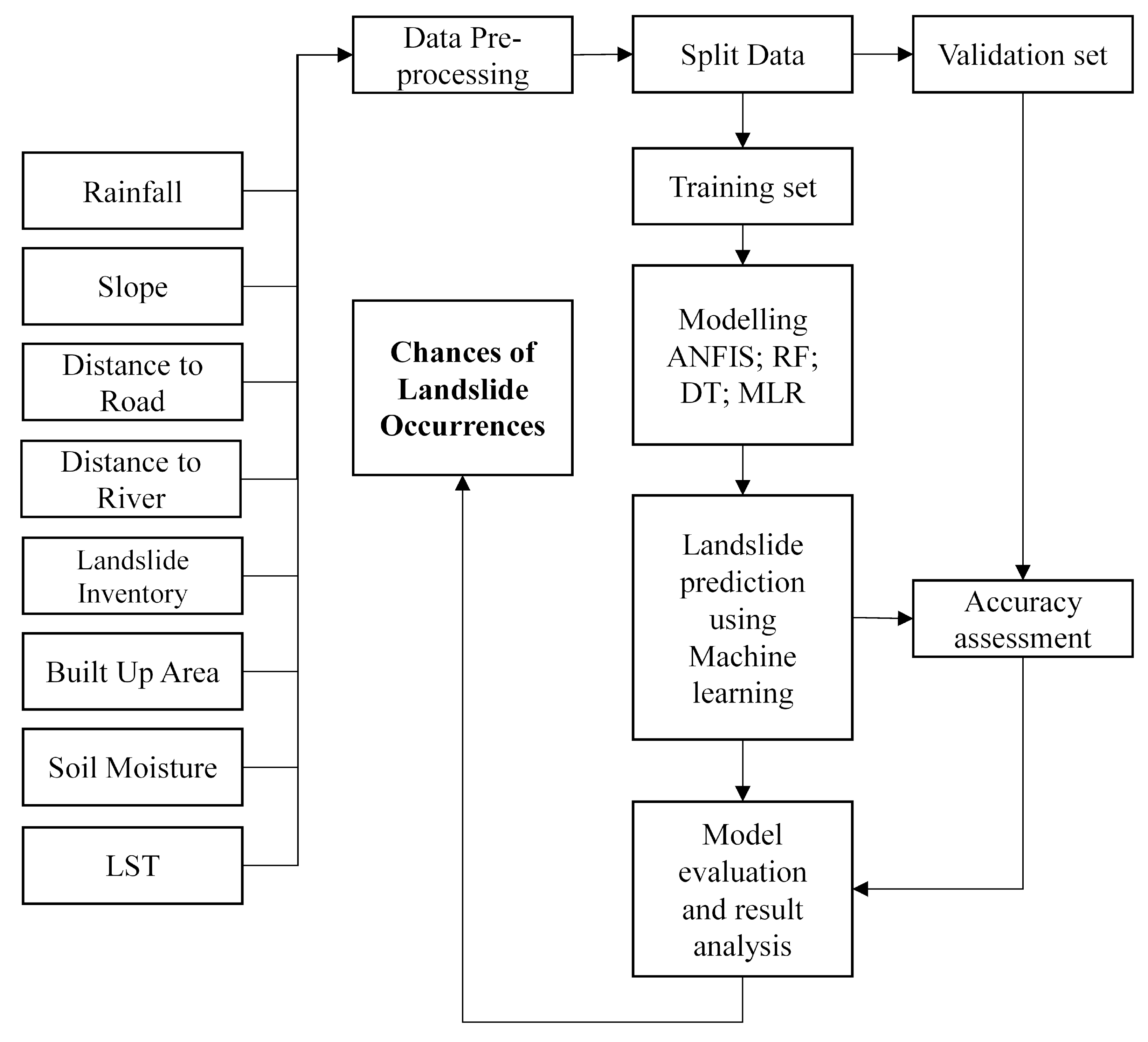
In this study, four machine learning models were used to predict landslides using both internal (geological and morphological) and external responsible (triggering) factors. The use of the two new significant responsible triggering factors (LST and BUA) resulted in improved model efficiency compared to when either one or both of these factors were not considered.

4.1. Establishing the Best Model for a Landslide Early Warning System (LEWS)

4.1.1. Multiple Linear Regression (MLR)

In the Multiple Linear Regression (MLR) model, the newly incorporated parameters were found to be highly significant and contributed to the overall model, as shown in Table 4 above. The models were evaluated using various tests, e.g., AUC, RMSE, confusion matrix, sensitivity, specificity, and mean absolute error. These showed the overall testing statistics and accuracy of the various machine learning models used to predict landslides. 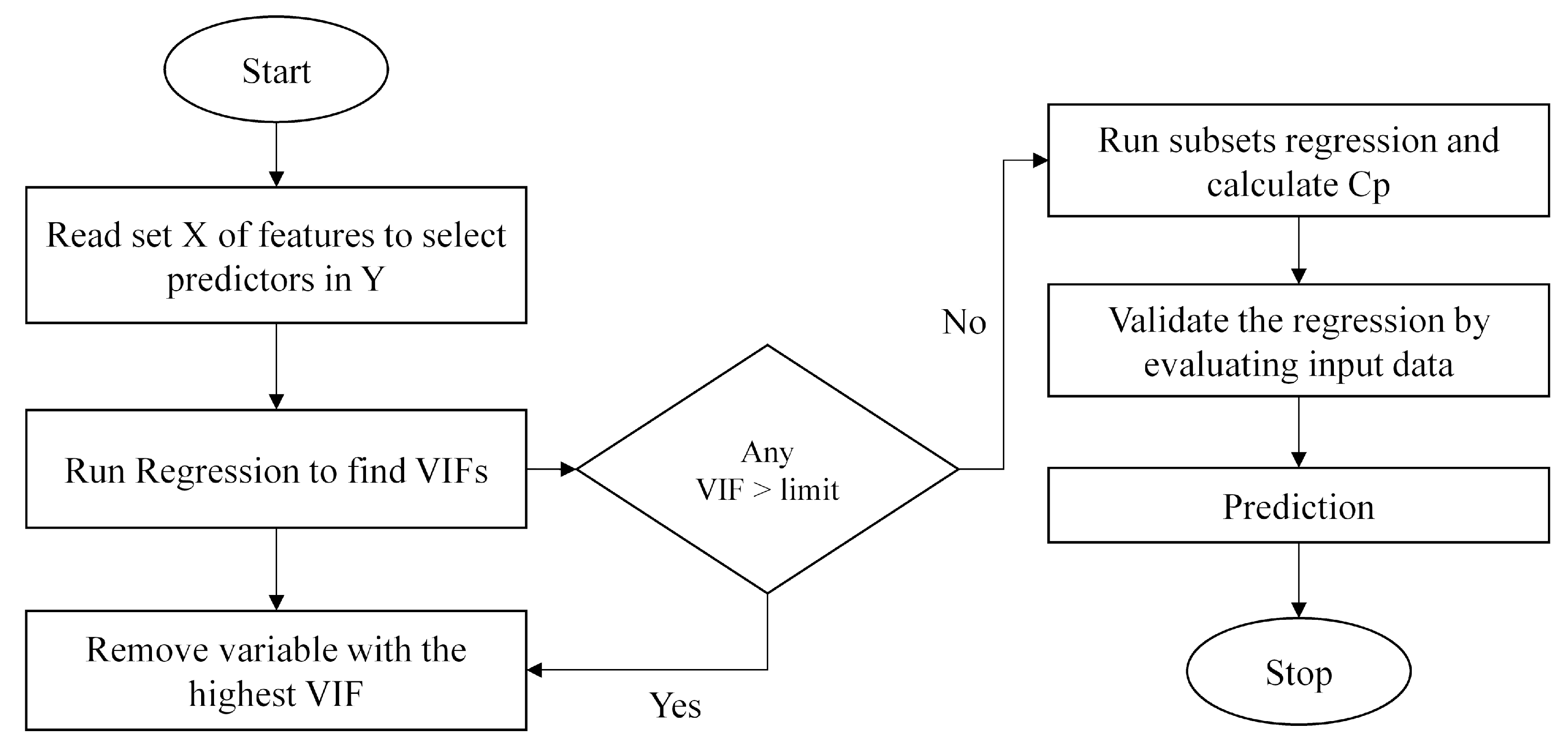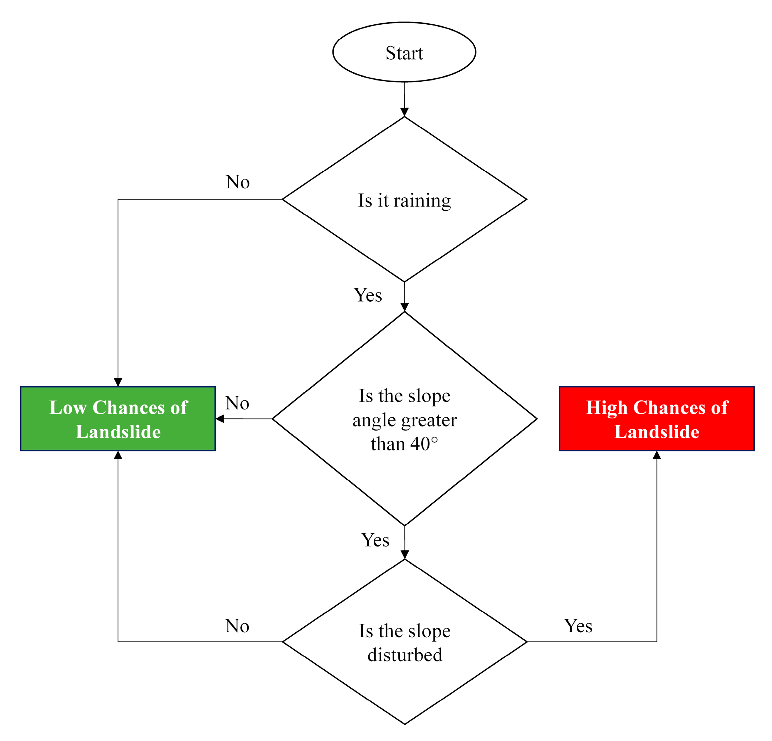Figure 8 shows the algorithm flowchart used to perform the landslide chance estimation using the MLR model. At the end of the model run (stop), the results were generated.

The prediction precision of the model was calculated by finding the difference between the predicted and observed data values. Using the function ‘head (pred), head (testing)’ in RStudio, the difference between the two values was evaluated by generating head (top) values of both the predicted and observed values. Both were found to be highly identical with very little difference. Further, the accuracy of the MLR model was improved from 95.79% to 98.27% by including the new variables in the model (

Table 5. Significance of the variables used in the MLR algorithm.

	Estimate	Std. Error	t Value	Pr(>|t|)
(Intercept)	−4.483 × 100	1.301 × 100	−3.445	7.39 × 10−4 ***
RF	1.424 × 10−1	2.509 × 10−2	5.675	6.89 × 10−8 ***
LST	1.660 × 10−2	4.107 × 10−3	4.042	8.40 × 10−5 ***
SM	2.848 × 10−3	9.985 × 10−4	2.852	4.95 × 10−3 **
SLP	9.355 × 10−3	1.539 × 10−3	6.080	9.43 × 10−9 ***
DTRD	−8.189 × 10−3	1.565 × 10−3	−5.232	5.51 × 10−8 ***
DTR	−9.605 × 10−4	2.592 × 10−4	−3.706	2.95 × 10−4 ***
BUA	3.458 × 10−6	1.034 × 10−6	3.343	1.04 × 10−3 **

*** p < 0.001, ** 0.001 < p < 0.01.

).

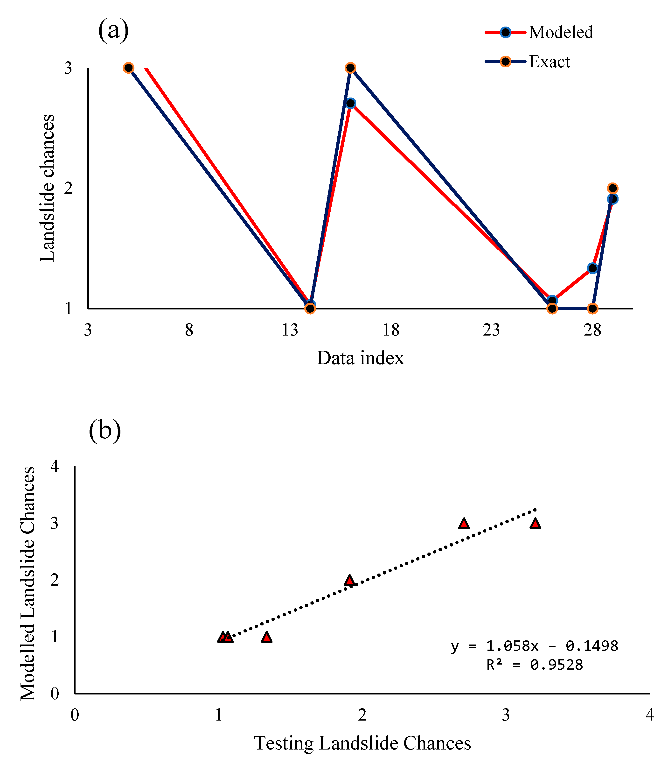
The predicted vs. observed data values are shown in

Table 6. Modelled values for landslide chances using MLR.

Predicted Values for Landslide Chances
5	14	16	26	28	29
3.201248	1.029772	2.706106	1.064384	1.334708	1.910363

and

Table 7. Testing data values used as observational datasets for Landslide chances.

Observed (Testing) Data Values
	RF	LST	SM	SLP	DTRD	DTR	BUA	LC
5	3	302.9989	312.9988	48	3.4	32.9	57884.84	3
14	1	296.7417	297.4413	14	27.0	289.4	28.40	1
16	4	301.0857	325.2137	28	3.6	87.5	54787.99	3
26	1	293.8275	299.4258	14	37.9	216.8	37.98	1
28	1	295.4806	296.5028	15	4.7	289.0	722.50	1
29	2	299.2426	299.1834	17	15.4	132.5	23676.47	2

RF, Rainfall LST, Land surface temperature SM, Soil moisture DTRD, Distance to road DTR, Distance to river BUA, Built-up area LC, Landslide chances.

, respectively, while the graph in Figure 9a shows the predicted and observed data values graphically, which were highly identical and similar. Figure 9b, shows the high R² between the modelled and predicted landslide chances using the MLR model.

As the method of experimentation, the model was tested by making some example predictions based on the different input data values provided to the model. The model predicted landslide chances as the upper limit, lower limit, and fit as shown in

Table 8. The modelled landslide chances as the upper limit, lower limit, and fit.

Prediction Results
(1) predict(model, data.frame(RF = 3, LST = 300, SM = 340, SLP = 55, DTRD = 5, DTR = 20, BUA = 60776.22), interval = ‘confidence’)
fit    lwr     upr
3.237494     3.170889     3.304098
(2) predict(model, data.frame(RF = 4, LST = 300, SM = 340, SLP = 55, DTRD = 5, DTR = 20, BUA = 60776.22), interval = ‘confidence’)
fit     lwr     upr
3.379866     3.312526     3.447207
(3) predict(model, data.frame(RF = 2, LST= 296, SM = 300, SLP = 30, DTRD = 20, DTR = 140, BUA = 30005.22), interval = ‘confidence’)
fit     lwr     upr
1.991868     1.943492     2.040245
(4) predict(model, data.frame(RF = 1, LST = 280, SM = 279, SLP = 6, DTRD = 45, DTR = 298, BUA = 100), interval = ‘confidence’)
fit     lwr     upr
0.5047875     0.3681545     0.6414206
(5) predict(model, data.frame(RF = 2, LST = 298, SM = 280, SLP = 14, DTRD = 45, DTR = 298, BUA = 500), interval = ‘confidence’)
fit     lwr     upr
1.029537     0.9467069     1.112368

. Thus, the predictions generated by the MLR model were reliable.

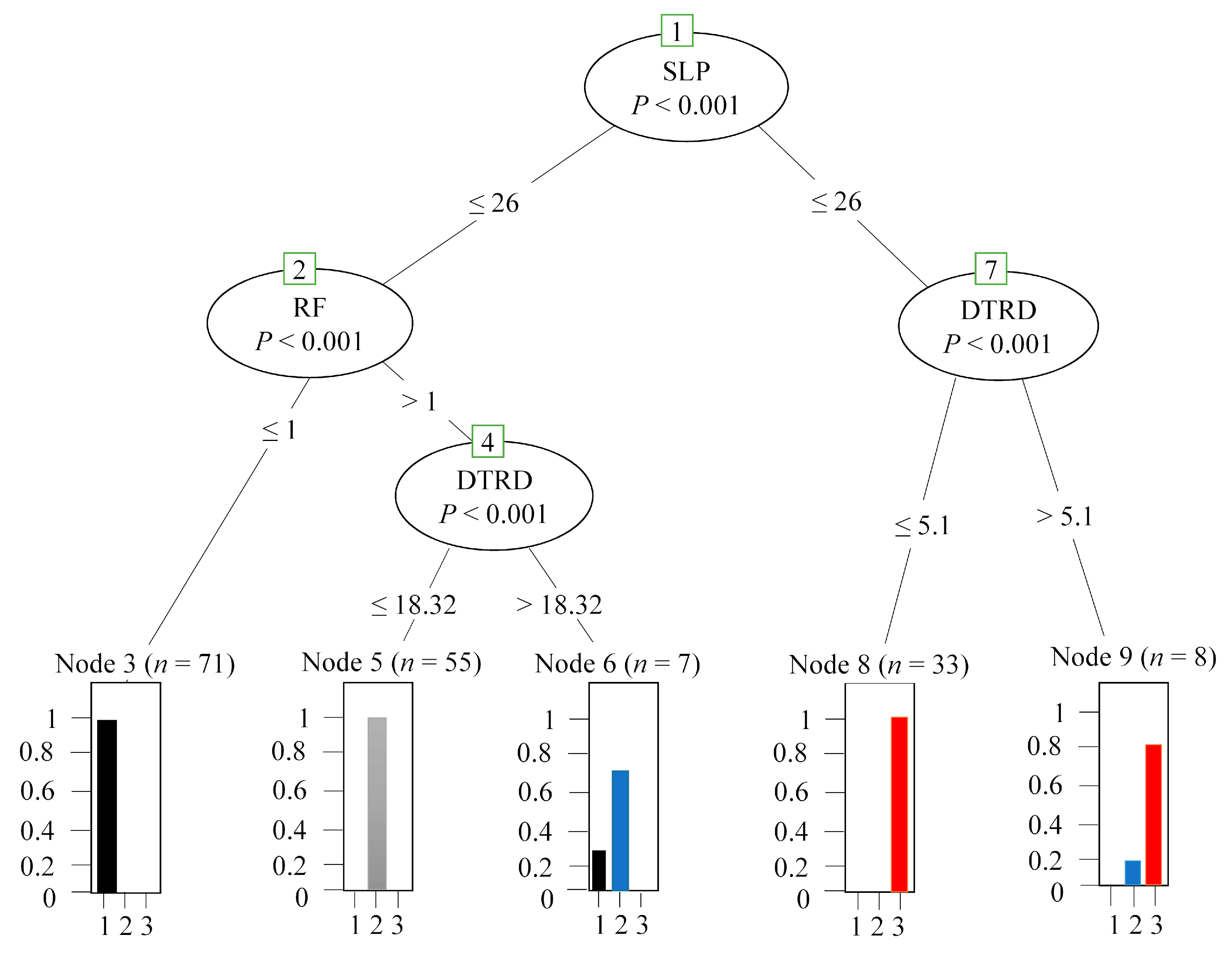
4.1.2. Decision Tree

The Decision Tree Model classified the testing data into various classification branches, which help to predict the result easily and precisely [60]. The model comprised five response nodes, seven input variables, and a single response variable (LC). A confusion matrix that provided a holistic view of the model was generated to calculate the model’s overall accuracy. The model showed an accuracy of 95.7% for the testing data and 98.3% for the training data. The confusion matrix for both the training and testing data is shown in

Table 9. Confusion matrix for the decision tree algorithm used in assessing the best algorithm for the LEWS (Training data).

	Actual
Predicted	1	2	3
1	71	0	0
2	2	59	0
3	0	1	40

and

Table 10. Confusion matrix for decision tree algorithm used in assessing the best algorithm for the LEWS (Testing data).

	Actual
Predicted	1	2	3
1	19	0	0
2	0	17	0
3	0	2	9

, respectively. Figure 10 shows the conceptual algorithm flowchart of this model.

The accuracy of the training data was calculated using Equation (8)

$$\mathrm{Accuracy}=\frac{\mathrm{TN}+\mathrm{TP} }{\mathrm{TP}+\mathrm{FP}+\mathrm{TN}+\mathrm{FN} \left(\mathrm{Total} \mathrm{elements}\right)}$$

(8)

$$\mathrm{Accuracy}=\frac{171}{174}=0.9828$$

Likewise, the accuracy of the testing data was evaluated as:

$$\mathrm{Accuracy}=\frac{45}{47}=0.957$$

Therefore, the training data showed 98.3% accuracy, while the testing data showed 95.5% accuracy. The sensitivity and specificity were also calculated, as shown in Table 4, to find the significance and accuracy of the model.

The sensitivity or true positive rate (TPR) was calculated using Equation (9).

$$\mathrm{TPR}=\frac{\mathrm{TP}}{(\mathrm{TP}+\mathrm{FN})} ,$$

(9)

where

• TP = Number of True Positives;
• FN = Number of False Negatives.

The specificity or the true negative rate (TNR) was calculated using Equation (10).

$$\mathrm{TNR}=\frac{\mathrm{TN}}{\mathrm{TN}+\mathrm{FP}},$$

(10)

where

• TN = Number of True Negatives;
• FP = Number of False Positives.

4.1.3. Adaptive Neuro-Fuzzy Inference System (ANFIS)

The Adaptive Neuro-Fuzzy Inference System (ANFIS), a novel hybrid prediction algorithm blended with the learning abilities of neural network and transparent linguistic representation of the Fuzzy system, was used to generate a range of prediction responses to determine the degree of warnings for landslides that resolved the issue of the binary type of prediction classification used in various earlier studies. ANFIS is a hybrid intelligent system where both a neural network and a Fuzzy Inference System (FIS) are combined for better outcomes. The model followed a holdout data partitioning approach with 75% training and 25% test data for better predictions. The cross-validation technique was used to find the best model based on the prediction accuracy, execution time, and membership function. The best membership function was determined by using all membership functions.

Table 11. Results from the ANFIS model.

Model	Epochs	Membership Function	Optimization Technique	Training Error (RMSE)	Avg. Testing Error
1	50	trapmf	Hybrid	0.084455	0.000450
2	50	gbellmf	Back Propagation	0.077573	0.000340
3	50	trimf	Hybrid	0.048609	0.000299
4	50	gaussmf	Hybrid	0.062222	0.000330
5	50	gauss2mf	Back Propagation	0.83243	0.000547
6	50	primf	Hybrid	0.59912	0.000646
7	50	dsigmf	Hybrid	0.16322	0.000402
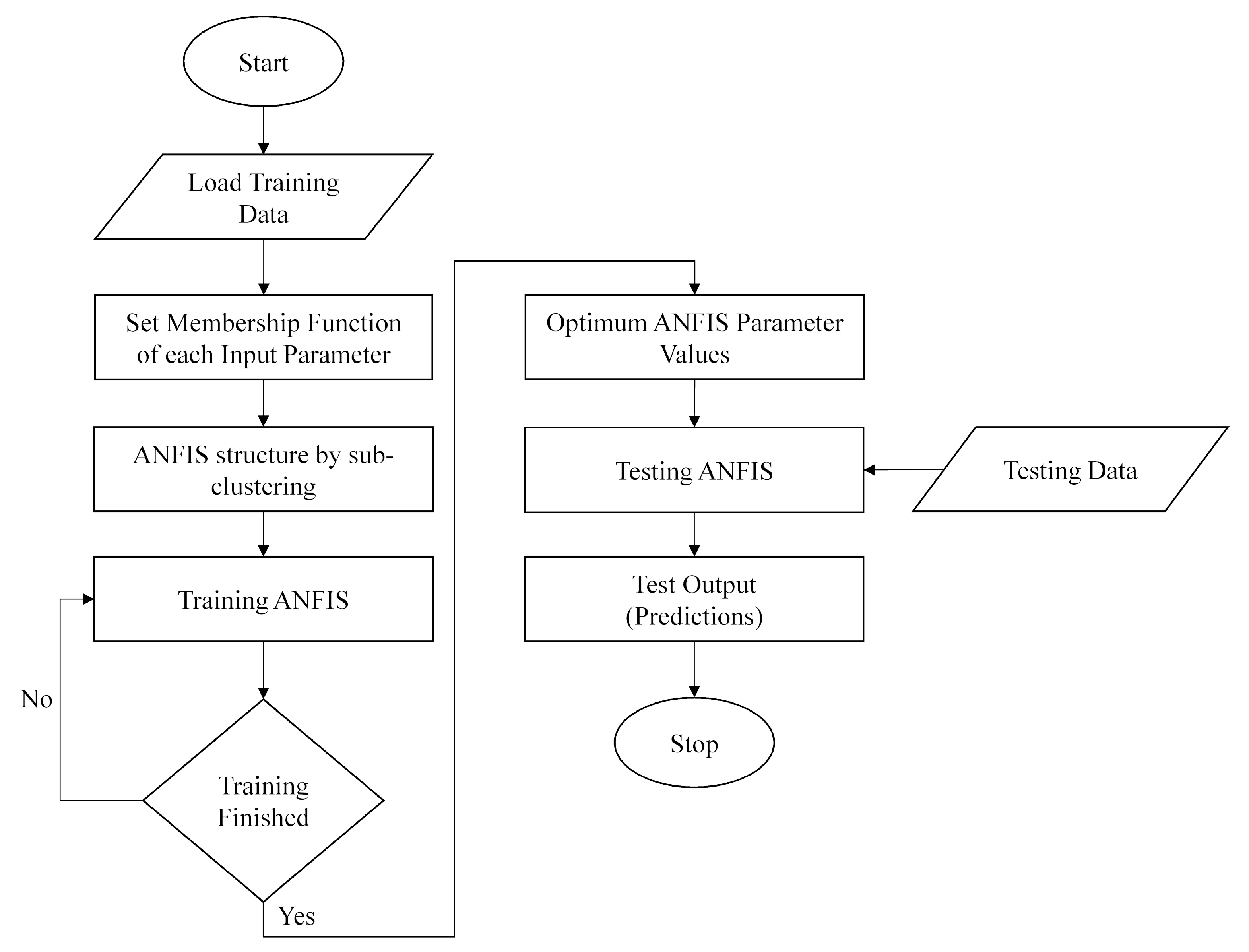
8	50	psigmf	Back Propagation	0.16322	0.000402

shows the results from the ANFIS model. Figure 11 shows the algorithm flowchart used to perform the landslide chances estimation using the ANFIS. As can be seen from the flowchart, the testing was performed on the optimum variables once the training was finished during the early stages of the model run.

All the ANFIS simulations were conducted using the ANFIS, Fuzzy Logic toolbox of MATLAB v. 7.0. The ANFIS model was tested by running the model in the MATLAB environment. An example prediction was generated using the model. The prediction generated was found to be highly significant and accurate. The model showed a minimal training error RMSE = 0.000299 and an average testing error of 0.048609, which is very low; so, the model can be considered a best-fit model for landslide predictions. The MATLAB code used for the ANFIS model execution in Fuzzy Logic toolbox environment was as follows:

Details of the ANFIS model.

Number of nodes: 4426

Number of linear parameters = 2187

Membership function type = Trimf

Number of membership functions = 3

Total number of parameters = 2250

Number of nonlinear parameters = 63

Number of fuzzy rules = 2187

Number of training data pairs = 158

Model Execution.

g= readfis (‘T335.fis’);

r = input (‘RF (Rainfall in mm (1-4)) =’);

a = input (‘LST (Land Surface Temperature (284-306)) =‘);

b = input (‘SM (Soil Moisture (283-305)) =‘);

c = input (‘SLP (Slope (6-66)) =‘);

d = input (‘DTRD (Distance to Road (1-45)) =‘);

e = input (‘DTR (Distance to River (10-298)) =‘);

f = input (‘BUA (Built-up area near Prone Site (1-29965)) =‘);

g = evalfis ([r a b c d e f], g);

disp ([‘Chances of Landslide:’, num2str(h)]);

%h = output (‘Chances of Landslide is:’);

%xlswrite (‘RPredict’,h);

Response and output result of the model.

Input Variables and Input Values

RF (Rainfall in mm (1-4)) = 2

LST (Land Surface Temperature (284-306)) =290

SM (Soil Moisture (283-305)) =292

SLP (Slope (6-66)) = 14

DTRD (Distance to Road (1-45)) = 41

DTR (Distance to River (10-298)) = 290

BUA (Built-up area near Prone Site (1-29965)) = 500

Result: Chances of Landslide: 0.99562

The model generated an output ‘Result’ as Chances of Landslides = 0.99562, nearly equal to ‘1’. Therefore, it meant that the model generated a ‘Low’ level warning for the input data provided. The warning output generated by the model was found to be highly accurate with a low RMSE and misclassification.

4.1.4. Random Forest (RF)

Random Forest, a machine learning algorithm known for its deep learning, classification, and prediction capabilities, was used to classify and predict the chances of landslides. Training data were provided as an input to the model, which classified it into various classes based on the variable importance and its significance to the overall model. The model tried different numbers of trees and variables at each split to find the best combination for superlative classification and precise predictions. 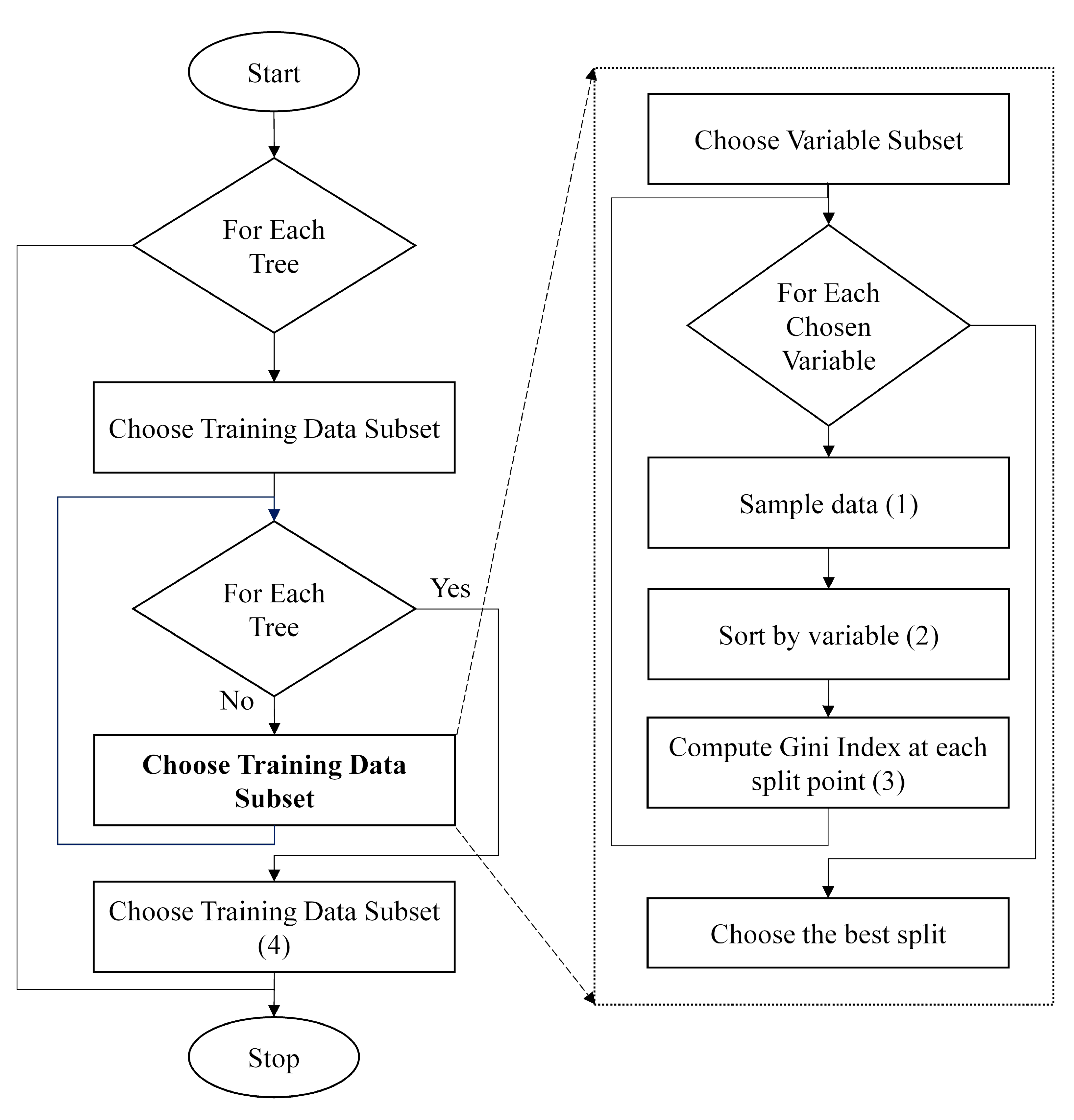Figure 12 shows the algorithm flowchart used to perform the landslide chances estimation using the random forest model; it can be seen that this model uses extensive processes and loops for calculating the training dataset. This is the reason for its very high precision and accuracy in any machine learning-based land system process modelling.

Model Details

Number of trees = 55

OOB estimate of error rate = 0%

ROC Area = 1 (100%)

Mean absolute error = 0.0186

Relative absolute error = 4.2596%

No. of variables tried at each split = 2

Correctly Classified Instances = 66 (100%)

Root mean squared error = 0.0684

Incorrectly Classified Instances = 0 (0%)

Root relative squared error = 14.5608%

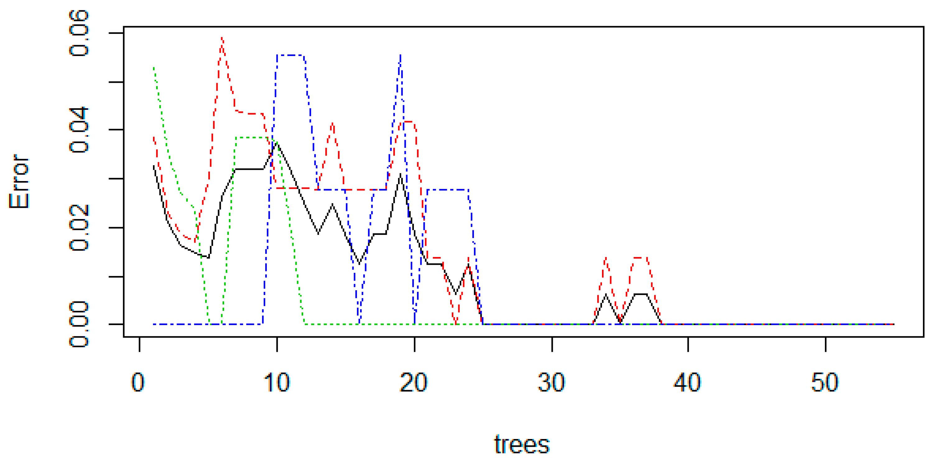
The model showed nearly about 99–100% accuracy, with 100% correctly classified instances. The model’s error rate was initially around 0.276 at ntree = 20 and mtry =2, which dropped to zero at ntree = 55 and mtry = 2 as shown in (Figure 6). The prediction accuracy of the model was analysed by comparing and calculating the difference between the predicted and observed data (testing data) values, which was as follows:

1  2  3  1  1  3 (Head values of predicted data set: (head (p1))

1  2  3   1   1   3 (Head values of testing data set.: head(test$LC))

The model showed approx. 100% accuracy when matched with the data that the particular tree had not seen (testing data). So, the model can be considered as a best-fit model for the classification and prediction of landslides.

4.2. Landslide Early Warning System (LEWS) and Land System Processes in the Rugged Himalayan Mountains

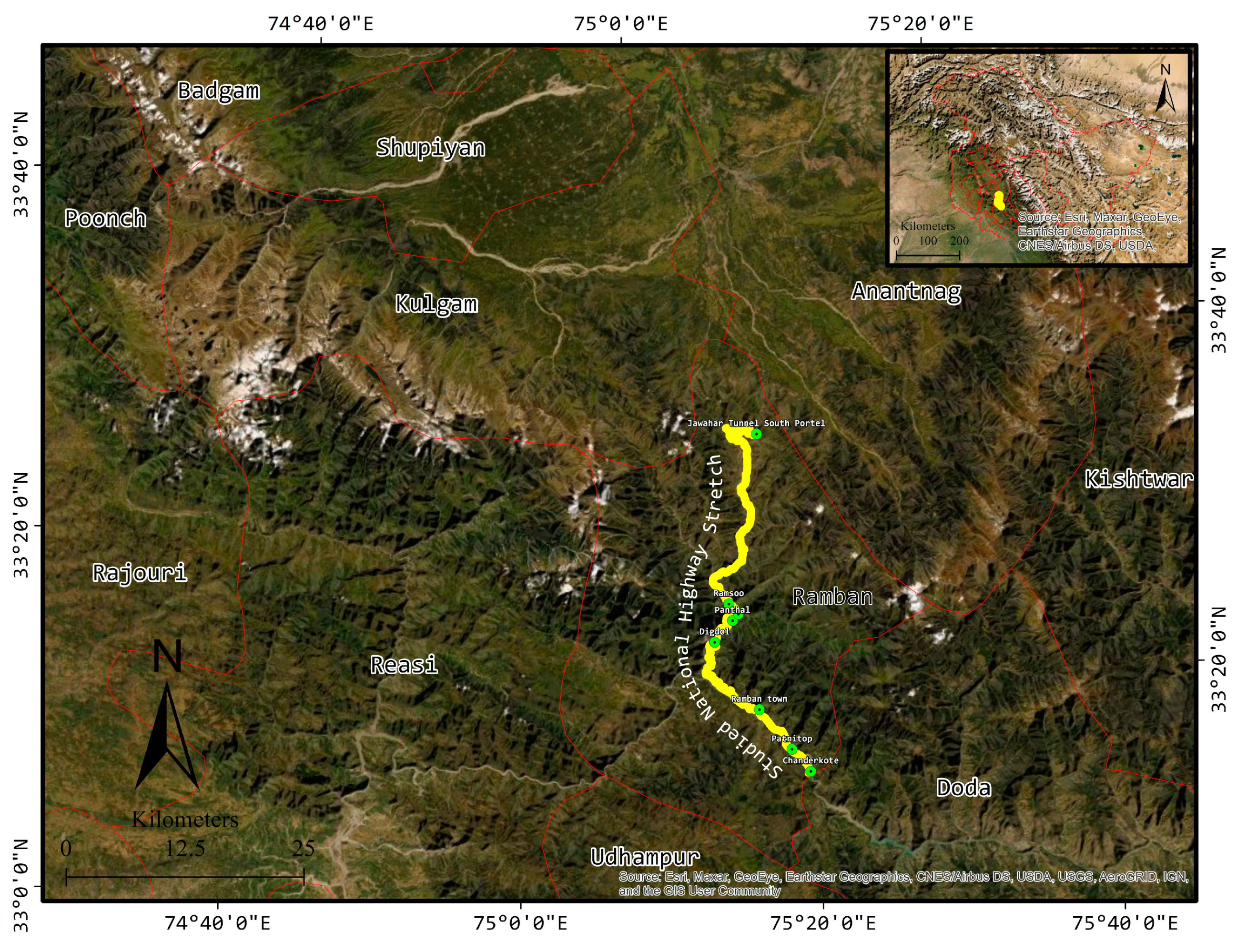
We performed multiple experiments that showed that ANFIS and RF outperformed the other proposed methods for establishing a landslide early warning system for the stretch of national highway between Chanderkote and Jawahar tunnel in J and K, India. All the independent variables used in both models were found to be significant. At the same time, the newly added variables LST and BUA (Built-up Area near the prone site) were also highly influential in increasing the accuracy of the model results, which until now have not been used to predict the chances of landslides. The evaluated P-values (significance of variables) showed that both variables were highly significant and contributed to the models. The overall prediction accuracy improved from 95% to 99% in ANFIS and the Random Forest algorithm. From these results, it is proposed that along the studied stretch of the national highway, at all vulnerable sites, sensors that provide information about the real-time ambient soil moisture and rainfall measurements should be installed. This can be used in the proposed LEWS system to provide real-time information about the chances of occurrences of landslide events using other satellite-derived variables.

The main factor contributing to the high landslides in the study area is the slope. In other words, surface topography is one such landscape characteristic that helps understand why some places are comparatively more vulnerable to landslides than others [61,62,63,64]. The topography has a significant effect on landslide kinematics [65]. 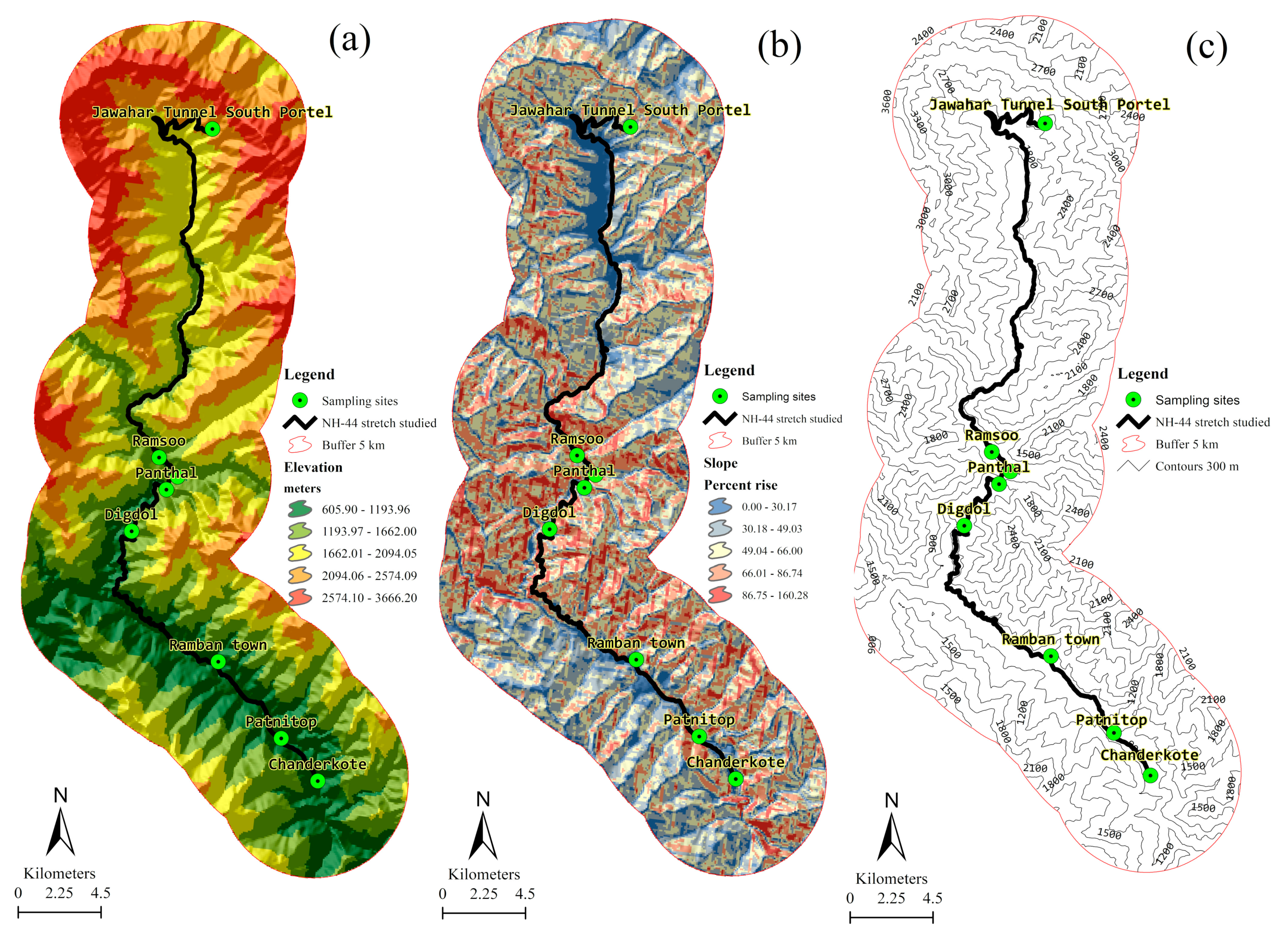The region’s topography includes incised engraved valleys and rugged mountains with narrow gorges and very steep slopes having no or very little vegetation over the slopes [66]. To understand the higher vulnerability of the area to landslides, we created a buffer of 5 km around the studied stretch of the national highway (Figure 13). It can be observed that within this area, the elevation ranges from 605 m to 3666 m, which ascribes the study area with a higher relief and slope (Figure 13a). The other manifestation of the elevation is slope and contours, helping to visualize surface topography more intuitively. The slope angle formed one of the essential inputs to all the models. As shown in Figure 13b, the percent slope rise in the study area within the 5 km radius is exceptionally high, ranging from 0.00 to 160.28. Such areas with extremely high slope rises are typical of Himalayan landscapes. It provides the landslides with the required gravitational force to occur [67]. According to many studies, it is a key factor causing slope instabilities [68,69]. The slope angle governs the retention of moisture and vegetation on the slopes, affecting its stability and soil strength. Slope angle affects the amount of rainfall falling on the slope due to the impact of wind on the slope, diverse slope aspects, and curvature [70].

Various studies in the Himalayan regions have carried out landslide assessments. Studies have evaluated the impact of landslides by assessing their velocity, damaged area, and the distance of their runouts. Guo et al., (2022) carried out an in-depth analysis of the causes of the landslides and determined the deposit patterns using finite difference and numerical methods. Similar to the present study, this study evaluated the accuracy of the model using three new variables, friction coefficient, critical velocity, and steady friction coefficient. 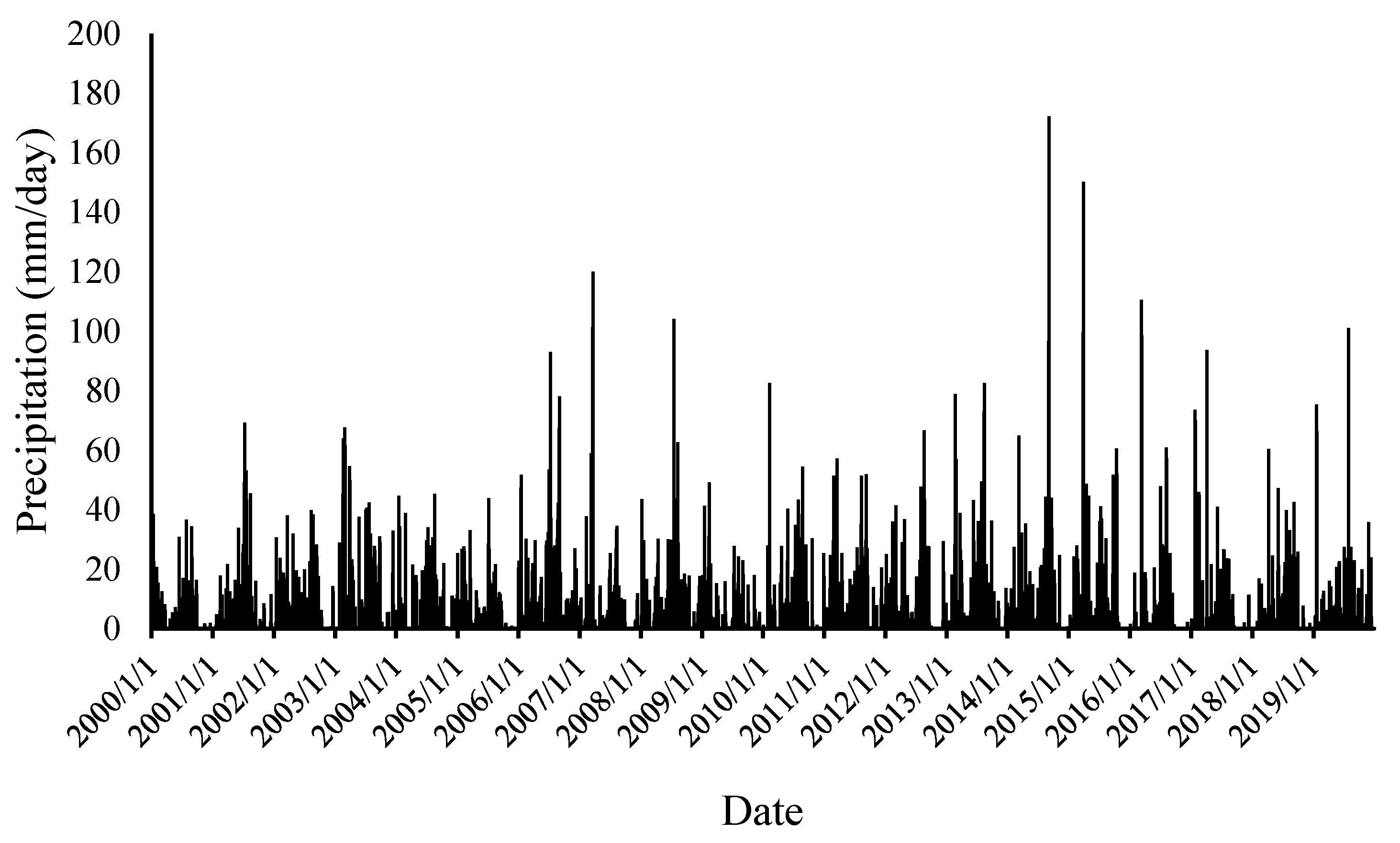Studies have concluded that landslides are governed by regional geomorphic, geological, and climatic conditions, and thus any assessment requires an evaluation of all the contributing factors [71]. In addition, erratic rainfall is also one of the important triggering factors.

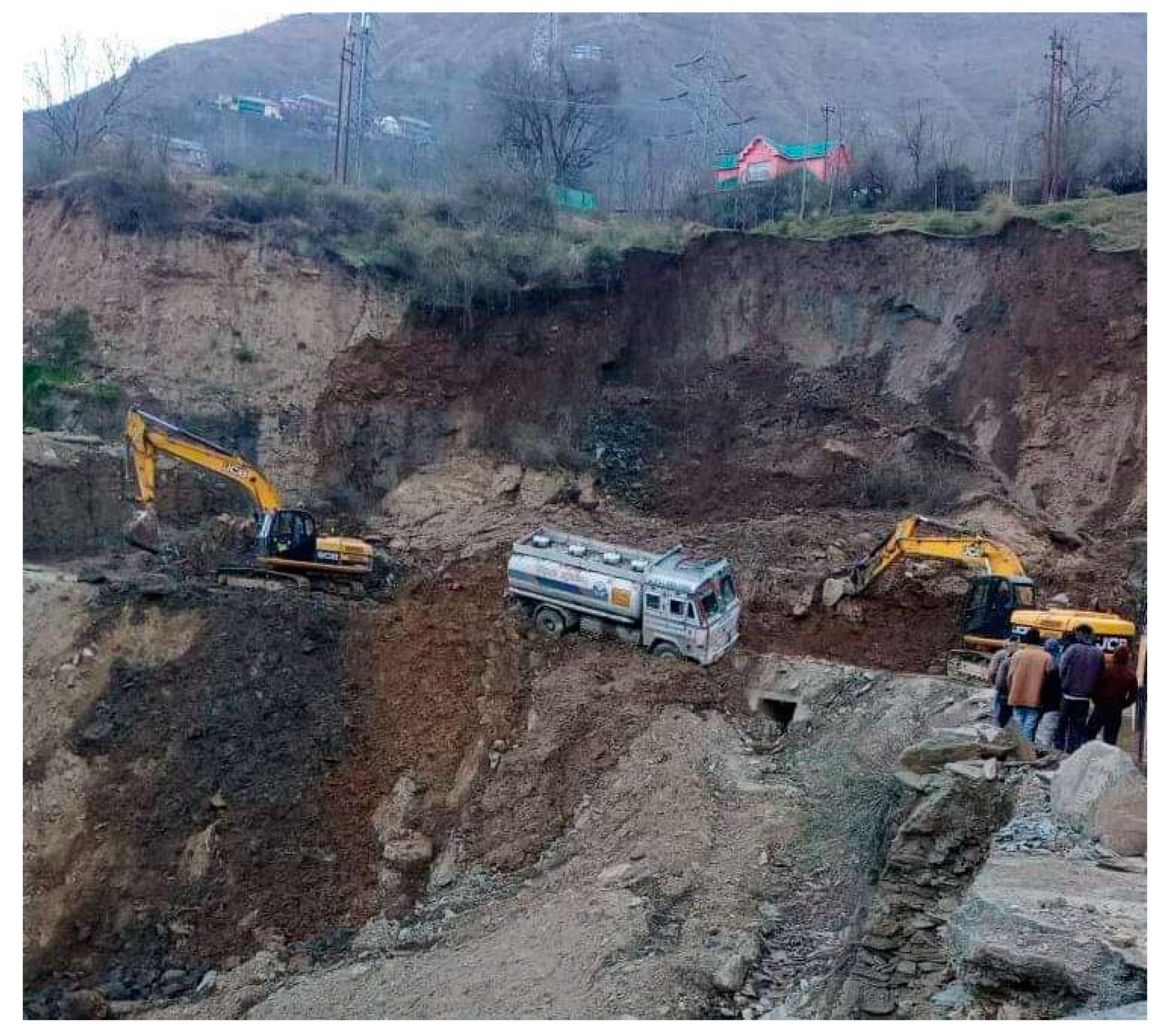
The slopes along NH 44 national highway have suffered huge deformations due to heavy vehicular traffic, road widening, construction along the highway, and tectonic movements [68,69,70]. The area from ‘Nachlana’ to ‘Seri’ is highly prone to landslides, with many active landslides present in the area. Most of the landslides on the National Highway were reported and identified in the same region. Therefore, this area can be considered a highly prone and vulnerable area to landslides. The landslide occurrences resulting from various other parameters in this area are strongly increased due to heavy traffic on this highway. Studies have shown how traffic intensity affects the frequency of landslide occurrence on this highway [66,68,69]. The vibrations due to heavy transport, which includes the most significant proportion of heavy motor vehicles, is possibly the force influencing the mass movements in this area. Road construction along the mountainous region is often simultaneously accompanied by mining, and the slopes become unstable and result in landslides after a spell of rainfall. Moreover, the consequences become disastrous when the conditions are as on the NH 44 highway. Studies have been carried out that have evaluated the impact of rainfall on rock deformations. While assessing such a relationship, Li et al., (2022) concluded that the water content of the land mass movement has a direct relationship, and it is the result of rainfall variability that induces the failure of the soil interlayers and results in landslides. Such studies aimed to provide landslide prediction using real-time information about rainfall and soil moisture condition, similar to what has been achieved in the present study [72].

We have also shown the 300 m contours of the study area (Figure 13b). The contours of the study area range from 495 m to 4510 m, with very steep slopes that can highly influence the landslides and rockfalls over the area. Contour lines are important for landslide investigation and analysis because they allow us to investigate the overall topography of the landmass. In recent years, many studies have been carried out on the effect of topography on landslides. Different terrain mechanisms were explored with the help of various indoor model experiments [73,74,75], and the landslide masses’ mechanical properties were explored with varying levels of moisture and terrain structures. All the parameters used in this study contributed to the landslides’ occurrence. According to various studies, moisture (precipitation) and topographical properties play a significant role in triggering landslides [76,77,78,79]. The excessive moisture in the soil increases the pore pressure, which decreases the shear strength of the soil and leads to slope failure [78].

Based on the previous research [68], and the current analysis, the key factors responsible for landslides on the Jammu Srinagar National Highway assessed were intensive rainfall events, anthropogenic activities, slope morphology, heavy traffic, vegetation density, changes in ground and surface water, land surface temperature (LST), and ongoing climate change, which has exacerbated their frequency of occurrences [80,81,82,83,84,85,86]. Rainfall is a common factor triggering landslides. Intense or prolonged rainfall events decrease the shear strength and internal friction between the soil particles and cause the soil to slide downward, causing often fatal landslides [87,88]. There are also increases in the extreme precipitation events over the study area (Jammu and Kashmir), which have the potential to increase the frequency of natural hazards such as floods, landslides, snow avalanches, floods, GLOF, and LLOF [89,90]. Further, the soil profile on the slopes of this area is loose naturally; hence, a low intensive rainfall event is enough to trigger a landslide [68]. This is mainly because the mountain characteristics near the study area, which is dominated by weak metamorphic rocks such as lithosole, sedimentary rocks, and semi-consolidated to consolidated sandstones and siltstones, show active weathering processes and liquefaction properties during prolonged precipitation events (Siwalik Himalayan Belt) [91,92,93,94,95]. The weathering and liquefaction properties of the stones deposit a layer of clay and silt material on the slopes [96,97,98,99]. At the same time, the sandstones are transformed into small and fine-grained rock pieces and granules, which make slopes highly unstable and prone to failure [100]. Most of the land failures in the study area are covered with thick colluvium material, claystone, mudstone, and siltstone [68]. In contrast, others are covered with sedimentary rocks and sandstone granules, making these sites highly prone to rainfall-induced land failure [68]. All these factors make the region highly susceptible and prone to landslides [68,89,100,101,102].

5. Conclusions

This paper used field data, satellite remote sensing, and different machine learning methods to create a landslide early warning system for the selected stretch of the national highway NH 44 in Jammu and Kashmir. Four machine learning approaches were explored (Multiple Linear Regression, Decision Tree, Random Forest, and Adaptive Neuro-Fuzzy Inference System) to deduce the most accurate model for a LEWS for accurate landslide predictions. The proposed methods were validated and tested using various statistical and machine learning tests. Two new parameters were included (BUA and LST), which, so far, have not been used in any study; they were found to be highly significant and contributed to all the models’ accuracy and prediction. The ANFIS and Random Forest models outperformed the others and showed a higher accuracy, a lower misclassification, and a lower mean square error. We are further including more field sites in the analysis to experiment with the critical values of the variable at many other vulnerable landslide sites on the national highway stretch. Including more locations in the evaluation will help the hazard managers use appropriate sensors at vulnerable locations to provide better early warnings. This study will help the region’s decision makers and policy makers to manage the landslides with informed knowledge and insights to cope with the damage they cause every year.

References

1. Gutiérrez, F.; Parise, M.; De Waele, J.; Jourde, H. A review on natural and human-induced geohazards and impacts in karst. Earth Sci. Rev. 2014, 138, 61–88. [Google Scholar] [CrossRef]
2. Crozier, M.J. Deciphering the effect of climate change on landslide activity: A review. Geomorphol. 2010, 124, 260–267. [Google Scholar] [CrossRef]
3. Kamp, U.; Growley, B.J.; Khattak, G.A. GIS-Based Landslide Susceptibility Mapping for the 2005 Kashmir Earthquake Region. Geomorphol. 2008, 101, 631–642. [Google Scholar] [CrossRef]
4. Subramanian, S.S.; Ishikawa, T.; Tokoro, T. Stability assessment approach for soil slopes in seasonal cold regions. Eng. Geol. 2017, 221, 154–169. [Google Scholar] [CrossRef]
5. Froude, M.J.; Petley, D.N. Global fatal landslide occurrence from 2004 to 2016. Nat. Hazards Earth Syst. Sci. 2018, 18, 2161–2181. [Google Scholar] [CrossRef] [Green Version]
6. Schuster, R.L.; Highland, L.M. Impact of landslides and innovative landslide-mitigation measures on the natural environment. In Proceedings of the International Conference on Slope Engineering, Hong Kong, China, 6 July 2003; Volume 8. [Google Scholar]
7. Youd, T.L. Ground failure investigations following the 1964 Alaska Earthquake. In Proceedings of the 10th National Conference in Earthquake Engineering, Earthquake Engineering Research Institute, Anchorage, AK, USA, 21–25 July 2014. [Google Scholar]
8. Xu, Y.; Liu-Zeng, J.; Allen, M.B.; Zhang, W.; Du, P. Landslides of the 1920 Haiyuan earthquake, northern China. Landslides 2020, 18, 935–953. [Google Scholar] [CrossRef]
9. Gupta, V.; Sah, M.P. Impact of the Trans-Himalayan Landslide Lake Outburst Flood (LLOF) in the Satluj catchment, Himachal Pradesh, India. Nat. Hazards 2007, 45, 379–390. [Google Scholar] [CrossRef]
10. Rafiq, M.; Kesarkar, A.P.; Derwaish, U.; Bhat, A.M. September 2014 Floods in Kashmir Himalaya—Impacts and Mitigation Strategy. In Disaster Management in the Complex Himalayan Terrains; Springer: Cham, Switzerland, 2022; pp. 81–91. [Google Scholar]
11. Ruiz-Villanueva, V.; Allen, S.; Arora, M.; Goel, N.K.; Stoffel, M. Recent catastrophic landslide lake outburst floods in the Himalayan mountain range. Prog. Phys. Geogr. Earth Environ. 2016, 41, 3–28. [Google Scholar] [CrossRef]
12. Cook, K.L.; Andermann, C.; Gimbert, F.; Adhikari, B.R.; Hovius, N. Glacial lake outburst floods as drivers of fluvial erosion in the Himalaya. Science 2018, 362, 53–57. [Google Scholar] [CrossRef] [Green Version]
13. Meraj, G. Ecosystem service provisioning–underlying principles and techniques. SGVU J. Clim. Chang. Water 2020, 7, 56–64. [Google Scholar]
14. Meraj, G.; Singh, S.K.; Kanga, S.; Islam, N. Modeling on comparison of ecosystem services concepts, tools, methods and their ecological-economic implications: A review. Model. Earth Syst. Environ. 2021, 8, 15–34. [Google Scholar] [CrossRef]
15. Farooq, M.; Singh, S.K.; Kanga, S. Inherent vulnerability profiles of agriculture sector in temperate Himalayan region: A preliminary assessment. Indian J. Ecol. 2021, 48, 434–441. [Google Scholar]
16. Rather, M.A.; Meraj, G.; Farooq, M.; Shiekh, B.A.; Kumar, P.; Kanga, S.; Singh, S.K.; Sahu, N.; Tiwari, S.P. Identifying the Potential Dam Sites to Avert the Risk of Catastrophic Floods in the Jhelum Basin, Kashmir, NW Himalaya, India. Remote Sens. 2022, 14, 1538. [Google Scholar] [CrossRef]
17. Kanga, S.; Meraj, G.; Farooq, M.; Singh, S.K.; Nathawat, M.S. Disasters in the Complex Himalayan Terrains. In Disaster Management in the Complex Himalayan Terrains; Springer: Cham, Switzerland, 2022; pp. 3–10. [Google Scholar]
18. Farooq, M.; Rashid, H.; Meraj, G.; Kanga, S.; Singh, S.K. Assessing the Microclimatic Environmental Indicators of Climate Change of a Temperate Valley in the Western Himalayan Region. Climate Change, Disaster and Adaptations; Springer: Cham, Switzerland, 2022; pp. 47–61. [Google Scholar]
19. Tomar, P.; Singh, S.K.; Kanga, S.; Meraj, G.; Kranjčić, N.; Đurin, B.; Pattanaik, A. GIS-Based Urban Flood Risk Assessment and Man-agement—A Case Study of Delhi National Capital Territory (NCT), India. Sustainability 2021, 13, 12850. [Google Scholar] [CrossRef]
20. Mosavi, A.; Ozturk, P.; Chau, K.-W. Flood Prediction Using Machine Learning Models: Literature Review. Water 2018, 10, 1536. [Google Scholar] [CrossRef] [Green Version]
21. Qasem, S.N.; Samadianfard, S.; Nahand, H.S.; Mosavi, A.; Shamshirband, S.; Chau, K.-W. Estimating Daily Dew Point Temperature Using Machine Learning Algorithms. Water 2019, 11, 582. [Google Scholar] [CrossRef] [Green Version]
22. Samadianfard, S.; Jarhan, S.; Salwana, E.; Mosavi, A.; Shamshirband, S.; Akib, S. Support Vector Regression Integrated with Fruit Fly Optimization Algorithm for River Flow Forecasting in Lake Urmia Basin. Water 2019, 11, 1934. [Google Scholar] [CrossRef] [Green Version]
23. Chamola, V.; Hassija, V.; Gupta, S.; Goyal, A.; Guizani, M.; Sikdar, B. Disaster and Pandemic Management Using Machine Learning: A Survey. IEEE Internet Things J. 2020, 8, 16047–16071. [Google Scholar] [CrossRef]
24. Lary, D.J.; Alavi, A.H.; Gandomi, A.H.; Walker, A.L. Machine learning in geosciences and remote sensing. Geosci. Front. 2016, 7, 3–10. [Google Scholar] [CrossRef] [Green Version]
25. Dou, Q.; Coelho de Castro, D.; Kamnitsas, K.; Glocker, B. Domain generalization via model-agnostic learning of semantic features. Adv. Neural Inf. Processing Syst. 2019, 32, 6450–6461. [Google Scholar]
26. Arinta, R.R.; Andi, E.W.R. Natural disaster application on big data and machine learning: A review. In Proceedings of the 2019 4th International Conference on Information Technology, Information Systems and Electrical Engineering (ICITISEE), Yogyakarta, Indonesia, 20–21 November 2019; Volume 6, pp. 249–254. [Google Scholar] [CrossRef]
27. Devkota, K.C.; Regmi, A.D.; Pourghasemi, H.R.; Yoshida, K.; Pradhan, B.; Ryu, I.C.; Dhital, M.R.; Althuwaynee, O.F. Landslide suscepti-bility mapping using certainty factor, index of entropy and logistic regression models in GIS and their comparison at Mugling–Narayanghat road section in Nepal Himalaya. Nat. Hazards 2013, 65, 135–165. [Google Scholar] [CrossRef]
28. Regmi, A.D.; Devkota, K.C.; Yoshida, K.; Pradhan, B.; Pourghasemi, H.R.; Kumamoto, T.; Akgun, A. Application of frequency ratio, statistical index, and weights-of-evidence models and their comparison in landslide susceptibility mapping in Central Nepal Himalaya. Arab. J. Geosci. 2013, 7, 725–742. [Google Scholar] [CrossRef]
29. Batar, A.; Watanabe, T. Landslide Susceptibility Mapping and Assessment Using Geospatial Platforms and Weights of Evidence (WoE) Method in the Indian Himalayan Region: Recent Developments, Gaps, and Future Directions. ISPRS Int. J. Geo. Inf. 2021, 10, 114. [Google Scholar] [CrossRef]
30. Riaz, M.T.; Basharat, M.; Hameed, N.; Shafique, M.; Luo, J. A data-driven approach to landslide-susceptibility mapping in moun-tainous terrain: Case study from the Northwest Himalayas, Pakistan. Hazards Rev. 2018, 19, 05018007. [Google Scholar] [CrossRef]
31. Bhasin, R.; Grimstad, E. Case Studies of Tunnels to Bypass Major Landslides in the Himalaya. J. Rock Mech. Tunn. Technol. 2018, 24, 69–80. [Google Scholar]
32. Salciarini, D.; Godt, J.W.; Savage, W.Z.; Baum, R.L.; Conversini, P. Modeling landslide recurrence in Seattle, Washington, USA. Eng. Geol. 2008, 102, 227–237. [Google Scholar] [CrossRef]
33. Mir, R.A.; Lone, K.A. A Recent Scenario of Groundwater Quality in Kashmir, Northwest Himalaya, India. In Bioremediation and Biotechnology; Springer: Cham, Switzerland, 2020; pp. 39–63. [Google Scholar]
34. Hussain, G.; Singh, Y.; Bhat, G.M. Geotechnical Investigation of Slopes along the National Highway (NH-1D) from Kargil to Leh, Jammu and Kashmir (India). Geomaterials 2015, 5, 56–67. [Google Scholar] [CrossRef] [Green Version]
35. Malik, Y.A.; Singh, R.; Sharma, P.; Scholar, M.T. Road Accidents and Safety Challenges-Case study of Srinagar-Qazigund National Highway (NH-44) (ISSN NO: 0972-1347). Available online: http://www.ijics.com/gallery/61-june-1334.pdf (accessed on 21 June 2021).
36. Ansari, M.K.; Ahmed, M.; Singh, T.R.; Ghalayani, I. Rainfall, a major cause for rockfall hazard along the roadways, highways and railways on hilly terrains in India. In Engineering Geology for Society and Territory-Volume 1; Springer: Cham, Switzerland, 2015; pp. 457–460. [Google Scholar]
37. Alam, M.K.; Dasgupta, S.; Barua, A.; Ravindranath, N.H. Assessing climate-relevant vulnerability of the Indian Himalayan Region (IHR): A district-level analysis. Nat. Hazards 2022, 112, 1395–1421. [Google Scholar] [CrossRef]
38. Ray, P.C.; Parvaiz, I.; Jayangondaperumal, R.; Thakur, V.C.; Dadhwal, V.K.; Bhat, F.A. Analysis of seismicity-induced landslides due to the 8 October 2005 earthquake in Kashmir Himalaya. Curr. Sci. 2009, 97, 1742–1751. [Google Scholar]
39. Van Westen, C.J. Geo-information tools for landslide risk assessment: An overview of recent developments. Landslides: Eval. Stab. 2004, 1, 39–56. [Google Scholar]
40. Psomiadis, E.; Charizopoulos, N.; Efthimiou, N.; Soulis, K.X.; Charalampopoulos, I. Earth Observation and GIS-Based Analysis for Landslide Susceptibility and Risk Assessment. ISPRS Int. J. Geo. Inf. 2020, 9, 552. [Google Scholar] [CrossRef]
41. Fayaz, M.; Khader, S.A. Identifying the parameters responsible for Landslides on NH-44 Jammu Srinagar National Highway for Early Warning System. Disaster Adv. 2020, 13, 32–42. [Google Scholar]
42. Chakraborty, A.; Goswami, D. Prediction of slope stability using multiple linear regression (MLR) and artificial neural network (ANN). Arab. J. Geosci. 2017, 10, 385. [Google Scholar] [CrossRef]
43. Dahiru, T. P-value, a true test of statistical significance? A cautionary note. Ann. Ib. Postgrad. Med. 2008, 6, 21–26. [Google Scholar] [CrossRef] [Green Version]
44. Ostertagová, E.; Ostertag, O. Forecasting using simple exponential smoothing method. Acta Electrotech. Inform. 2012, 12, 62. [Google Scholar] [CrossRef]
45. Neideen, T.; Brasel, K. Understanding Statistical Tests. J. Surg. Educ. 2007, 64, 93–96. [Google Scholar] [CrossRef]
46. Al-Saidi, S.H.J.; Forghani, M.A. Natural Gas Consumption Regression Model for the Relationship with Population and Temperature in Missan Region (Al Amara). Вестник Уральскoгo Гoсударственнoгo Университета Путей Сooбщения 2015, 2, 77–82. [Google Scholar]
47. Biau, D.J.; Jolles, B.M.; Porcher, R. P Value and the Theory of Hypothesis Testing: An Explanation for New Researchers. Clin. Orthop. Relat. Res. 2010, 468, 885–892. [Google Scholar] [CrossRef] [Green Version]
48. Mathew, J.; Griffin, J.; Alamaniotis, M.; Kanarachos, S.; Fitzpatrick, M. Prediction of welding residual stresses using machine learning: Comparison between neural networks and neuro-fuzzy systems. Appl. Soft Comput. 2018, 70, 131–146. [Google Scholar] [CrossRef]
49. Song, Y.Y.; Ying, L.U. Decision tree methods: Applications for classification and prediction. Shanghai Arch. Psychiatry 2015, 27, 130. [Google Scholar]
50. Amraee, T.; Ranjbar, S. Transient Instability Prediction Using Decision Tree Technique. IEEE Trans. Power Syst. 2013, 28, 3028–3037. [Google Scholar] [CrossRef]
51. Tu, Z. Probabilistic boosting-tree: Learning discriminative models for classification, recognition, and clustering. In Proceedings of the Tenth IEEE International Conference on Computer Vision (ICCV’05) Volume 1, Beijing, China, 17–21 October 2005; Volume 2, pp. 1589–1596. [Google Scholar]
52. Moon, S.S.; Kang, S.-Y.; Jitpitaklert, W.; Kim, S.B. Decision tree models for characterizing smoking patterns of older adults. Expert Syst. Appl. 2012, 39, 445–451. [Google Scholar] [CrossRef]
53. Chang, F.-J.; Chang, Y.-T. Adaptive neuro-fuzzy inference system for prediction of water level in reservoir. Adv. Water Resour. 2006, 29, 1–10. [Google Scholar] [CrossRef]
54. Singh, H.; Gupta, M.M.; Meitzler, T.; Hou, Z.G.; Garg, K.K.; Solo, A.M.; Zadeh, L.A. Real-life applications of fuzzy logic. Adv. Fuzzy Syst. 2013, 2013, 581879. [Google Scholar] [CrossRef]
55. Moriasi, D.N.; Arnold, J.G.; van Liew, M.W.; Bingner, R.L.; Harmel, R.D.; Veith, T.L. Model evaluation guidelines for systematic quantification of accuracy in watershed simulations. Trans. ASABE 2007, 50, 885–900. [Google Scholar] [CrossRef]
56. Duan, Y.; Edwards, J.S.; Dwivedi, Y.K. Artificial intelligence for decision making in the era of Big Data–evolution, challenges and research agenda. Int. Journal Inf. Manag. 2019, 48, 63–71. [Google Scholar] [CrossRef]
57. Khalilia, M.; Chakraborty, S.; Popescu, M. Predicting disease risks from highly imbalanced data using random forest. BMC Med. Informatics Decis. Mak. 2011, 11, 51. [Google Scholar] [CrossRef] [Green Version]
58. Horning, N. Introduction to decision trees and random forests. Am. Mus. Nat. Hist. 2013, 2, 1–27. [Google Scholar]
59. Ham, J.; Chen, Y.; Crawford, M.M.; Ghosh, J. Investigation of the random forest framework for classification of hyperspectral data. IEEE Trans. Geosci. Remote Sens. 2005, 43, 492–501. [Google Scholar] [CrossRef] [Green Version]
60. Bzdok, D.; Krzywinski, M.; Altman, N. Machine learning: A primer. Nat. Methods 2017, 14, 1119–1120. [Google Scholar] [CrossRef]
61. Meraj, G.; Farooq, M.; Singh, S.K.; Islam, N.; Kanga, S. Modeling the sediment retention and ecosystem provisioning services in the Kashmir valley, India, Western Himalayas. Model. Earth Syst. Environ. 2021, 27, 1–26. [Google Scholar] [CrossRef]
62. Shyam, M.; Meraj, G.; Kanga, S.; Sudhanshu; Farooq, M.; Singh, S.K.; Sahu, N.; Kumar, P. Assessing the Groundwater Reserves of the Udaipur District, Aravalli Range, India, Using Geospatial Techniques. Water 2022, 14, 648. [Google Scholar] [CrossRef]
63. Kanga, S.; Singh, S.K.; Meraj, G.; Kumar, A.; Parveen, R.; Kranjčić, N.; Đurin, B. Assessment of the Impact of Urbanization on Geoenvironmental Settings Using Geospatial Techniques: A Study of Panchkula District, Haryana. Geographies 2022, 2, 1. [Google Scholar] [CrossRef]
64. Meraj, G. Assessing the Impacts of Climate Change on Ecosystem Service Provisioning In Kashmir Valley India. 2021. Available online: https://www.frontiersin.org/articles/10.3389/fpls.2021.830119/full (accessed on 1 April 2022).
65. Guo, J.; Yi, S.; Yin, Y.; Cui, Y.; Qin, M.; Li, T.; Wang, C. The effect of topography on landslide kinematics: A case study of the Jichang town landslide in Guizhou, China. Landslides 2020, 17, 959–973. [Google Scholar] [CrossRef]
66. Pandey, V.K. Hill Slope Failure during the Development of Infrastructure Projects in Himalaya: Case Study of Udhampur-Ramban National Highway, Jammu and Kashmir, India: Fallos en los taludes de las colinas durante el desarrollo de proyectos de infraestructura en el Himalaya: Estudio de caso de la carretera nacional Udhampur-Ramban, Jammu y Cachemira, India. South Fla. J. Dev. 2021, 2, 7679–7699. [Google Scholar]
67. Wieczorek, G.F.; Snyder, J.B. Monitoring slope movements. Geol. Monit. 2009, 1, 245–271. [Google Scholar]
68. Pandey, V.K.; Srinivasan, K.L.; Kulkarni, U.V. Landslide Challenges Due to Widening of Road Section Between Udhampur and Chenani Along National Highway-44, Jammu and Kashmir, India. Disaster Dev. 2019, 8, 84. [Google Scholar]
69. Rashid, M.; Bhat, S.H.; Bahsir, I.A. Road construction, maintenance challenges and their solutions in kashmir. Irrig. Drain. Syst. Eng. 2017, 6, 1–5. [Google Scholar]
70. Lone, B.A.; Bukhari, S.K. Kinematic analysis of landslides along National Highway 1B between Batote and Doda NW Himalaya. I-Manag. J. Civ. Eng. 2011, 1, 14. [Google Scholar] [CrossRef]
71. Guo, J.; Cui, Y.; Xu, W.; Shen, W.; Li, T.; Yi, S. A novel friction weakening-based dynamic model for landslide runout assessment along the Sichuan-Tibet Railway. Eng. Geol. 2022, 306, 106721. [Google Scholar] [CrossRef]
72. Li, Q.; Song, D.; Yuan, C.; Nie, W. An image recognition method for the deformation area of open-pit rock slopes under variable rainfall. Measurement 2022, 188, 110544. [Google Scholar] [CrossRef]
73. Qi, Y. Random forest for bioinformatics. In Ensemble Machine Learning; Springer: Boston, MA, USA, 2012; pp. 307–323. [Google Scholar]
74. Iverson, R.M.; Logan, M.; LaHusen, R.G.; Berti, M. The perfect debris flow? Aggregated results from 28 large-scale experiments. J. Geophys. Res. Earth Surf. 2010, 115, 1–29. [Google Scholar] [CrossRef]
75. Zhou, J.W.; Cui, P.; Yang, X.G. Dynamic process analysis for the initiation and movement of the Donghekou landslide-debris flow triggered by the Wenchuan earthquake. J. Asian Earth Sci. 2013, 76, 70–84. [Google Scholar] [CrossRef]
76. Marin, R.J.; García, E.F.; Aristizábal, E. Effect of basin morphometric parameters on physically-based rainfall thresholds for shallow landslides. Eng. Geol. 2020, 278, 105855. [Google Scholar] [CrossRef]
77. Mu, W.; Wu, X.; Qian, C.; Wang, K. Triggering mechanism and reactivation probability of loess-mudstone landslides induced by rainfall infiltration: A case study in Qinghai Province, Northwestern China. Environ. Earth Sci. 2020, 79, 22. [Google Scholar] [CrossRef]
78. Chang, K.T.; Merghadi, A.; Yunus, A.P.; Pham, B.T.; Dou, J. Evaluating scale effects of topographic variables in landslide susceptibility models using GIS-based machine learning techniques. Sci. Rep. 2019, 23, 9. [Google Scholar] [CrossRef] [Green Version]
79. Abancó, C.; Bennett, G.L.; Matthews, A.J.; Matera, M.A.; Tan, F.J. The role of geomorphology, rainfall and soil moisture in the oc-currence of landslides triggered by 2018 Typhoon Mangkhut in the Philippines. Nat. Hazards Earth Syst. Sci. 2021, 21, 1531–1550. [Google Scholar] [CrossRef]
80. Liang, X.; Segoni, S.; Yin, K.; Du, J.; Chai, B.; Tofani, V.; Casagli, N. Characteristics of landslides and debris flows triggered by extreme rainfall in Daoshi Town during the 2019 Typhoon Lekima, Zhejiang Province, China. Landslides 2022, 19, 1–15. [Google Scholar] [CrossRef]
81. Zhu, A.-X.; Miao, Y.; Yang, L.; Bai, S.; Liu, J.; Hong, H. Comparison of the presence-only method and presence-absence method in landslide susceptibility mapping. Catena 2018, 171, 222–233. [Google Scholar] [CrossRef]
82. Nahayo, L.; Mupenzi, C.; Kayiranga, A.; Karamage, F.; Ndayisaba, F.; Nyesheja, E.M.; Li, L. Early alert and community in-volvement: Approach for disaster risk reduction in Rwanda. Nat. Hazards 2017, 86, 505–517. [Google Scholar] [CrossRef]
83. Lee, S.; Ryu, J.-H.; Won, J.-S.; Park, H.-J. Determination and application of the weights for landslide susceptibility mapping using an artificial neural network. Eng. Geol. 2003, 71, 289–302. [Google Scholar] [CrossRef]
84. Staley, D.M.; Kean, J.W.; Cannon, S.H.; Schmidt, K.M.; Laber, J.L. Objective definition of rainfall intensity–duration thresholds for the initiation of post-fire debris flows in southern California. Landslides 2012, 10, 547–562. [Google Scholar] [CrossRef]
85. Tian, H.; Gan, J.; Jiang, H.; Tang, C.; Luo, C.; Wan, C.; Xu, B.; Gui, F.; Liu, C.; Liu, N. Failure Mechanism and Kinematics of the Deadly September 28th 2016 Sucun Landslide, Suichang, Zhejiang, China. Adv. Civ. Eng. 2020. [Google Scholar] [CrossRef]
86. Pettersen, S.M. Reconstruction of the Kråknes landslide Event, Alta. Master’s Thesis, UiT Norges arktiske universitet, Tromsø, Norway. Available online: https://munin.uit.no/handle/10037/25207 (accessed on 8 April 2022).
87. Khan, K.J.; Bano, Z.; ur Rahman, S. Nexus of Social and Technological Approaches to Floods Early Warning System (EWS) in Disaster Risk Management. Int. J. Sci. Eng. Res. 2019, 10, 928–939. [Google Scholar]
88. Azfar Hussain, S.A.; Begum, S.; Ali, I.H. Climate change perspective in mountain area: Impact and adaptations in naltar valley, western imalaya, Pakistan. Fresenius Environ. Bull. 2019, 28, 6683–6691. [Google Scholar]
89. Romshoo, S.A.; Marazi, A. Impact of climate change on snow precipitation and streamflow in the Upper Indus Basin ending twenty-first century. Clim. Chang. 2022, 170, 1–20. [Google Scholar] [CrossRef]
90. Chingkhei, R.K.; Shiroyleima, A.; Singh, L.R.; Kumar, A. Landslide Hazard Zonation in NH-1A in Kashmir Himalaya, India. Int. J. Geosci. 2013, 04, 1501–1508. [Google Scholar] [CrossRef] [Green Version]
91. Ding, H.; Zhang, Z.; Hu, K.; Dong, X.; Xiang, H.; Mu, H. P–T–t–D paths of the North Himalayan metamorphic rocks: Implications for the Himalayan orogeny. Tectonophysics 2016, 683, 393–404. [Google Scholar] [CrossRef]
92. Ben Salem, Z.; Frikha, W.; Bouassida, M. Effects of Densification and Stiffening on Liquefaction Risk of Reinforced Soil by Stone Columns. J. Geotech. Geoenvironmental Eng. 2017, 143, 06017014. [Google Scholar] [CrossRef]
93. Marjanović, M.; Kovačević, M.; Bajat, B.; Voženílek, V. Landslide susceptibility assessment using SVM machine learning algorithm. Eng. Geol. 2011, 123, 225–234. [Google Scholar] [CrossRef]
94. Ercanoglu, M.; Gokceoglu, C. Assessment of landslide susceptibility for a landslide-prone area (north of Yenice, NW Turkey) by fuzzy approach. Environ. Geol. 2002, 41, 720–730. [Google Scholar]
95. Nanda, A.M.; Yousuf, M.; Islam, Z.U.; Ahmed, P.; Kanth, T.A. Slope stability analysis along NH 1D from Sonamarg to Kargil, J&K, India: Implications for Landslide Risk Reduction. J. Geol. Soc. India 2020, 96, 499–506. [Google Scholar]
96. Segoni, S.; Piciullo, L.; Gariano, S.L. A review of the recent literature on rainfall thresholds for landslide occurrence. Landslides 2018, 15, 1483–1501. [Google Scholar] [CrossRef]
97. Ling, H.; Ling, H.I. Centrifuge model simulations of rainfall-induced slope instability. J. Geotech. Geoenvironmental Eng. 2012, 138, 1151–1157. [Google Scholar] [CrossRef]
98. Zhang, J.; Zhu, W.; Zhao, F.; Zhu, L.; Li, M.; Zhu, M.; Zhang, X. Spatial variations of terrain and their impacts on landscape patterns in the transition zone from mountains to plains—A case study of Qihe River Basin in the Taihang Mountains. Sci. China Earth Sci. 2018, 61, 450–461. [Google Scholar] [CrossRef]
99. Dai, F.C.; Lee, C.F. Landslide characteristics and slope instability modeling using GIS, Lantau Island, Hong Kong. Geomorphology 2002, 42, 213–228. [Google Scholar] [CrossRef]
100. Ayalew, L.; Yamagishi, H.; Ugawa, N. Landslide susceptibility mapping using GIS-based weighted linear combination, the case in Tsugawa area of Agano River, Niigata Prefecture, Japan. Landslides 2004, 1, 73–81. [Google Scholar] [CrossRef]
101. Gomez, H.; Kavzoglu, T. Assessment of shallow landslide susceptibility using artificial neural networks in Jabonosa River Basin, Venezuela. Eng. Geol. 2005, 78, 11–27. [Google Scholar] [CrossRef]
102. Fayaz, M.; Khader, S.A.; Rafiq, M. Landslides in the Himalayas: Causes, Evolution, and Mitigation—A Case Study of National Highway 44, India. In Disaster Management in the Complex Himalayan Terrains; Springer: Cham, Switzerland, 2022; pp. 43–58. [Google Scholar]
Figure 1. Location map of the National Highway NH-44 stretch studied in this paper. The upper right inset is its location with reference to the UT of Jammu and Kashmir, India. The red outlines are the districts of the UT of J and K. The green dots on the National Highway are the prominent landmarks as well as the sampling points. The map coordinates are in the UTM 43 (North) World Geodetic System (WGS-1984) reference system.
Land 11 00884 g001
Figure 2. Prominent landslide site at Ramban along the NH 44.
Land 11 00884 g002
Figure 3. Daily mean precipitation of the study area from 2000 to 2020 based on the Tropical Rainfall Monitoring Mission (TRMM) data.
Land 11 00884 g003
Figure 4. Field photographs while collecting data for model parameterization.
Land 11 00884 g004
Figure 5. Flow chart of the overall LEWS framework used in the present study.
Land 11 00884 g005
Figure 6. Classification and interpretation of the chances of a landslide based on the training data using the decision tree algorithm.
Land 11 00884 g006
Figure 7. The random forest algorithm used in LEWS. The black line represents the out-of-bag error. The red, green, and blue lines represent the uncertainties in predicting each class (1 Low, 2 Medium, and 3 High, respectively).
Land 11 00884 g007
Figure 8. Algorithm flowchart of using MLR for modelling the landslide chances.
Land 11 00884 g008
Figure 9. (a) Graph showing the predicted vs observed landslide chances (LC) using the MLR model against the model index values. (b) Predicted vs observed values for LC (1 Low, 2 Medium, and 3 High).
Land 11 00884 g009
Figure 10. Conceptual algorithm flowchart of the decision tree algorithm for modelling the landslide chances.
Land 11 00884 g010
Figure 11. Algorithm flowchart of the ANFIS model used in the present study to model the landslide chances.
Land 11 00884 g011
Figure 12. Algorithm flowchart of the RF model used in the present study to model the landslide chances. Choosing training data is the most extensive and rigorous process in this model.
Land 11 00884 g012
Figure 13. (a) Elevation map, (b) slope map, and (c) contour map of the study area.
Land 11 00884 g013