Abstract
Rapid urbanization is causing changes in green spaces and ecological connectivity. So far, urban ecosystem research has mainly focused on using landscape metrics (LM) in two-dimensional (2D) space. Our study proposes three-dimensional (3D) measures of urban forests (UF) and LM calculations using LiDAR technology. First, we estimated the UF volume of Krakow (Poland) and the distribution of vegetation (low, medium, high) using a voxel-based GEOBIA approach based on the ALS LiDAR point cloud, satellite imagery, and aerial orthophotos at specific timestamps: 2006, 2012, 2017. Then, the appropriate landscape metrics were selected (NP, AREA_MN, CONTIG_MN, LPI, PARA_MN, SPLIT, MESH, PD, DIVISION, LSI) to quantify the differences between the 2D- and 3D-derived vegetation structures and detect changes in the urban landscape. The results showed that areas with low vegetation decreased due to the expansion of built-up areas, while areas with medium and high vegetation increased in Krakow between 2006, 2012, and 2017. We have shown that the lack of information on the vertical features of vegetation, i.e., 2D greenery analysis, leads to an overestimation of landscape connectivity. In the 3D vegetation classes, it was observed that low vegetation was the best connected, followed by high vegetation, while medium vegetation was dispersed in the city space. These results are particularly relevant for the urban environment, where the distribution of green space is crucial for the provision of ecosystem services.
1. Introduction
The urban landscape is a complex mosaic of different man-made land covers. Invested areas and green spaces try to fulfill their functions, which, at the same time, are more or less suited as habitats for various species of plants and animals. Human activity and urban management decisions have profoundly affected cities’ ecosystem functions [1,2]. Contemporary urban sprawl brings about numerous transformations in the structure and functioning of the cityscape. Recently raised themes in the analysis of urban landscapes in relation to the pressure of development and, hence, the growth of urbanization are the reduction of green spaces, habitats fragmentation, and the amplification of the mosaic character of the landscape [3,4,5,6]. However, this is undoubtedly a considerable simplification. The characteristics of landscape patterns are most often performed using landscape metrics (LM), which primarily quantify the spatial structure, i.e., the composition (the number and amount of different habitat types) and configuration (the spatial arrangement) of patch-based, discrete land cover classes within a geographic area [7,8]. For this purpose, over a hundred landscape metrics were developed for categorical data [9,10,11,12,13]. The FRAGSTATS [14] and the later GIS software such as the GuidosToolbox [15] were designed to compute a wide variety of LM. As researchers increasingly turn to R, a new ’landscapemetrics’ package, an extensive collection of widely used LM becomes more popular [16]. In recent decades, interpreting these metrics has become an important research topic in landscape ecology [17], as well as in relation to the cityscape [18], sustainable development [19], the monitoring of land cover changes [20,21,22], and urban or regional planning [23]. Recent research has also shown the need to emphasize multi-scale interactions in landscape pattern studies, suggesting methods for big data analysis [24].
The most often considered terms in the urban landscape, especially in the urban green space aspect, are habitat fragmentation and connectivity—key attributes of their spatial structure [25]. Fragmentation is the breaking up of a habitat or vegetation type into smaller, disconnected sections [26]. Connectivity indicates the degree to which the movement of species is facilitated or hindered between fragments in the landscape [27]. The method of their evaluation is the selection and construction of appropriate metrics, because one single parameter is not sufficient to explain complex fragmentation processes, which has been shown in many studies [28,29]. The choice of specific LM for a given problem is not easy and requires careful consideration of the potential application and data used. However, some of them, such as the Number of Patch (NP), Patch Density (PD), Mean Patch Area (AREA_MN), Mean Shape Index (SHAPE_MN), and Shannon’s Diversity Index (SHDI) have been widely adopted by researchers as the fundamental landscape configuration metrics [30]. Subsequent studies have proposed that the Effective Mesh Index (MESH), Splitting Index (SPLIT), and Landscape Division Index (DIVISION) should be added to the basic metrics in urban green space fragmentation analyses because of their reduced sensitivity to the presence of tiny residual patches [31,32]. Considering the measures of connectivity or fragmentation, high-resolution data are suitable for the analysis of heterogeneous urban areas, while medium-resolution data are more applicable in urban peripheries and suburban zones, where larger patches of green space are present and less fragmentation is perceived [26].
In recent years, a number of authors have shown in their work that the monitoring of urban green spaces and inventory methods with the determination of specific parameters of urban forests can be effectively supported by digital photogrammetry technologies and remote sensing, which enable the determination of urban vegetation characteristics at different levels of detail and scales [33]. However, research on the fragmentation and changes in urban green space using landscape metrics has primarily focused on its quantification from a two-dimensional (2D) perspective, most often using satellite or aerial orthophotos to classify vegetation and other classes, or based on available Land Use and Land Cover (LULC) maps, such as CORINE Land Cover (Copernicus) data [34,35,36]. A wide range of remote sensing platforms offering multi-resolution imageries, such as Landsat TM (30 m GSD—Ground Sample Distance), Sentinel-2 (10 m GSD), RapidEye (5.0 m GSD), SPOT-7 (1.5 m GSD PAN), Pleaides (0.5 m GSD PAN), and Worldview-3 (0.3 m GSD PAN)—along with geoinformatics techniques such as pixel-based classification, Geographic Object-Based Image Analysis (GEOBIA), or machine learning—were used to generate land use and land cover maps and deliver the LM [37,38,39,40,41]. Simultaneously, attempts showed that increasing the object details allows for a more precise definition of landscape features (objects) and provides a comprehensive assessment of the cause–effect relationships between classes [42]. However, there are some limitations in traditional 2D landscape models. This is problematic, especially in urban greenery due to the heterogeneous complexity of the vegetation canopy with diversified spatial and volumetric distribution. Because many living organisms do not just move horizontally (in 2D space) but also using multiple strata of the complex vegetation, it is therefore important to understand the spatial distribution of vegetation in three-dimensional (3D) space and characterize their metrics, which also has implications for determining the ecosystem services (ES) provided by urban forests (UF).
In recent years, the 3D biometrical parameters and volume of UF have started to be characterized in studies using LiDAR (Light Detection and Ranging) technology. The Airborne Laser Scanning (ALS) solution uses the time difference between the laser pulse emitted from a sensor in the air and the returning signal from the vegetation (trunk, branch stems, leaves), ground, or other object surface. Based on the travel time of the laser, the angles of the LiDAR platform, and their true coordinates (POS – GNSS + IMU; Position and Orientation System), the coordinates (x,y,z) of the objects can be calculated, obtaining a 3D point cloud, which can be processed (after ground classification) into a raster-based Digital Terrain Model (DTM) approximating the bare ground and the Digital Surface Model (DSM), representing tree canopies, roofs of buildings, and other objects such as ground and roads [43,44,45]. The processing of the next echo’s returning by the ground and vegetation most often results in the generation of a Canopy Height Model (CHM), which represents the normalized height of trees and shrubs. The CHM can also be used for tree and shrub extent detection and the measurement of 3D characteristics (e.g., the base of the crown height, the volume of the crown) [46,47]. Recently, based on the LiDAR point cloud, the urban landscape was presented in the 3D form using voxels (volumetric pixels) to calculate the volume of UF [48,49,50]. With the proliferation of 3D methods, the development of landscape metrics is also expanding into three dimensions, which could become a new paradigm in landscape science [51]. However, 3D LM are not ready to be widely used in urban landscape ecological studies [52]. Although Casalegno et al. conducted an analysis of ecological connectivity in 3D space in 2017 [53], there has been no further research on the spatiotemporal change of landscape metrics in such 3D environments. This is understandable given the heterogeneous structure of urban habitats and the challenges of acquiring adequate and comparable 3D data from different time periods to separate built-up areas from green infrastructure and classify different vegetation levels.
The purpose of the presented study was to measure the horizontal (2D) and vertical spatial distribution (3D) of green infrastructure and estimate the volume of the urban forest of Krakow (Poland) at specific timestamps—2006, 2012, and 2017—for the change detection in urban green spaces and the analyses of environmental impact using landscape metrics based on ALS LiDAR and Very High Resolution (VHR) satellite imagery. We also aimed to investigate how the 3D perspective affects landscape fragmentation indicators over time and space by comparing LM at a 2D level and when using 3D data, where low, medium, and high vegetation layers were distinguished.
2. Materials and Methods
2.1. Study Area
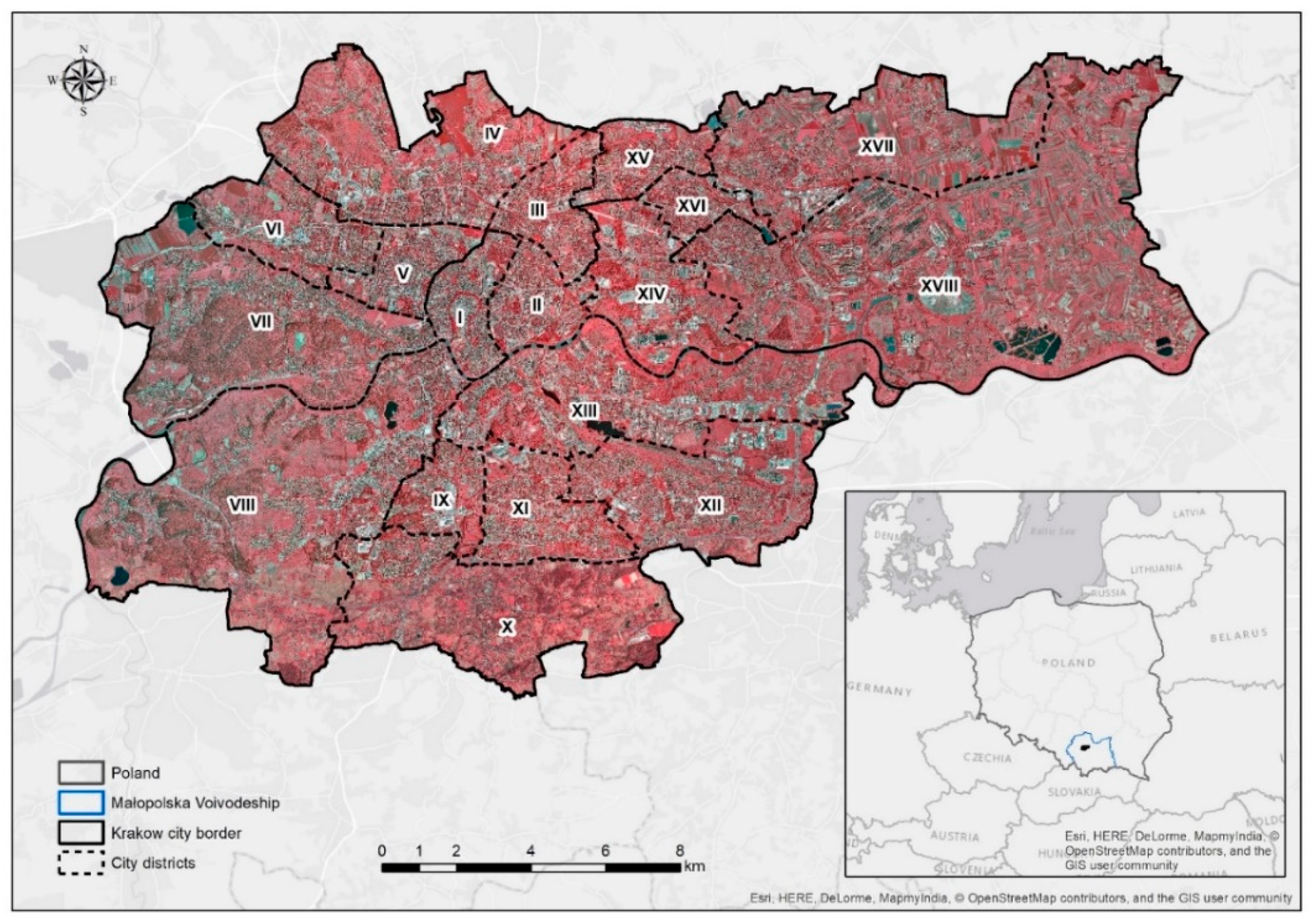
The study was conducted in Krakow, the second largest city located in South Poland (Lesser Poland Voivodeship), a cultural, academic, and touristic center with a total area of 327 km² and a population of about 782 thousand people, which is still growing [54]. The Krakow municipality is divided into 18 districts (Figure 1) which exhibit variability in the patterns of green infrastructure and architecture. As in other developing cities, Krakow’s major challenges include significant air pollution, urban sprawl and residential development, and a reputation for diminishing green space. The greatest threats to the formation of a coherent system of green areas in Krakow are external factors—legal conditions and investment pressure.

Figure 1.
Location of the study area on the base map of Europe and aerial orthophoto (CIR) of the Krakow municipality with district borders.
Krakow was chosen as a research object because of the intensive changes that have been taking place in urban tissue in recent years, which are putting pressure on various areas in the city. Although the current spatial structure of urban forests has been shaped by natural conditions and the development of the urban structure, for which the territorial expansion of the city, its contemporary multicentricity, and changing geometric shape are responsible, in the conceptual designs and implementation of shaping plans, the green areas of Krakow have been compared with model solutions [55]. Therefore, we had the opportunity to compare these concepts of connection with the existing spatial state in the research framework.
2.2. Input Data
Investigating the vegetation changes occurring in time and space (3D) at different landscape levels required the use of multi-temporal and multi-source spatial data. In this study, to prepare 2D and 3D UF maps, we used airborne laser scanning (ALS) point clouds acquired for the Krakow municipality area in 2006, 2012, and 2017 and VHR satellite imagery and aerial digital orthophotos acquired close to the dates of the LiDAR data acquisition (Table 1).

Table 1.
Details of the geospatial data acquired.
In 2006, the ALS LiDAR campaign was commissioned by the Municipality of Krakow (Office of Spatial Planning) and was performed in the fall after the end of the vegetation season (leaf-off period). This was the second application of ALS in Poland and the first study with such a high point density—at least 12 pts/m2 (RMSE: XY = 8 cm; Z = 5 cm) [56]. The ALS LiDAR point clouds acquired in 2012 and 2017 (cloud density ≥ 12 pts/m2, Standard II) [57] were obtained from Poland’s Central Office of Geodesy and Cartography; (projects: ISOK and CAPAP). The acquired 3D ALS point clouds were classified according to the ASPRS (American Society for Photogrammetry and Remote Sensing) standard, i.e., class 2—ground, 3—low vegetation (0.0–0.4 m above ground; AGL), 4—medium vegetation (0.4–2.0 m AGL), 5—high vegetation (2.0 max Z), 6—buildings (H > 2.0 m with specific planarity and surface parameters of the roof).
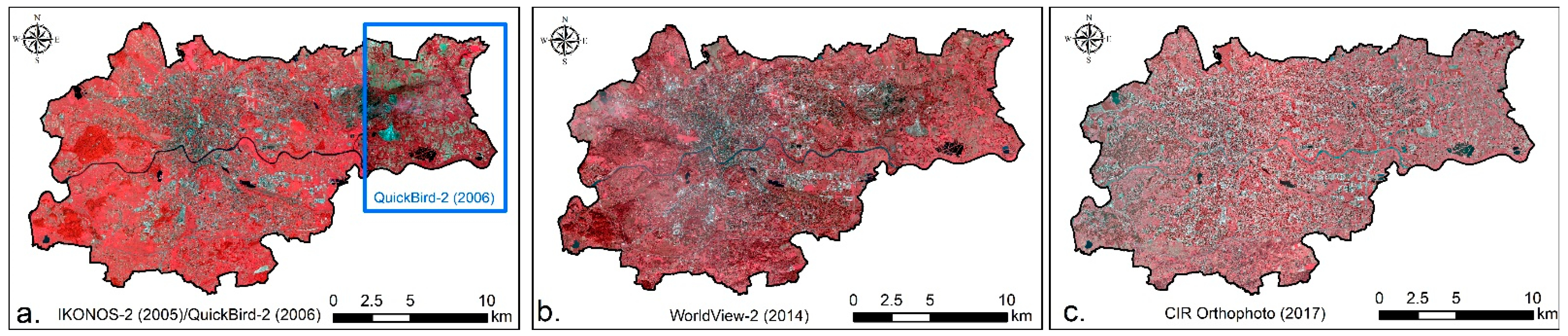
Available multispectral (MS) satellite imageries were used to analyze the green spaces, mainly including near-infrared (NIR) and red bands, because healthy vegetation has a high reflectance in NIR spectra and a low reflectance in red bands (high absorption by chlorophyll). In 2006, QuickBird-2 satellite imagery at 0.61 m (panchromatic—PAN) and at 2.4 m (multispectral—MS) resolutions was used to classify UF in the eastern part of the Krakow city, and IKONOS-2 (0.8 m PAN/3.2 m MS) from 2005 was used for the western part. For 2012, the green space classification was supported with available WorldView-2 imagery (0.5 m PAN/2.0 m MS) acquired in 2014 (closest available to ALS LiDAR 2012), and in 2017, Color-InfraRed (CIR) aerial orthophotos with 0.25 m GSD were used (Figure 2).
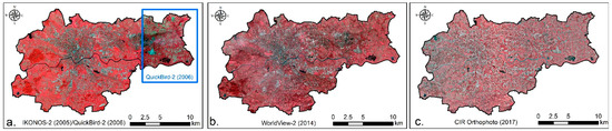
Figure 2.
Krakow in false-color imagery using the near infrared (NIR), red, and green spectral bands—this image shows vegetation in a red tone, as vegetation reflects most light in the NIR; (a) IKONOS-2 (2005) and QuickBird-2 (2006); (b) WorldView-2 (2014); and (c) CIR aerial orthophoto (2017).
2.3. Processing 2D and 3D Data
In order to analyze the landscape structure at different levels, in the first step, we created a land cover (LC) map of the vegetation in a raster format, which is necessary for quantifying the landscape metrics. We prepared both traditional 2D green space maps and vertical vegetation strata based on LiDAR 3D point clouds (namely, low, medium, and high vegetation). Additionally, we used a voxel-based approach to estimate changes in the volume of vegetation. The above analyses were applied to the 2006, 2012, and 2017 data sets.
The 2D maps with the distribution of green spaces/biologically active areas (BAA) were derived based on satellite imagery or CIR aerial orthophotos using spectral reflectance in the NIR and red band to calculate the Normalized Difference Vegetation Index (NDVI) [58]. The NDVI index reaches a value range from −1.0 to 1.0 and was used to separate class vegetated areas from built-up or other vegetation-free areas in the city. The index value thresholds were set based on histograms [59] and indicate the presence of vegetation (0.2 ≤ NDVI ≤ 1.0) or the absence of vegetation (−1.0 ≥ NDVI > 0.2). This analysis stage resulted in general 2D biologically active area (2D BAA) maps from NDVI, showing the spatial extent of urban vegetation. The created raster maps were resampled to a spatial resolution of 1.0 m.
The 3D LiDAR point clouds were used to classify the vegetation in the three separate vertical layers to estimate the impact of vertical stratification on the landscape metrics and their changes. Initially, the ALS LiDAR point cloud required pre-processing. We generated a 1.0 m GSD raster representing the Digital Terrain Model (DTM) and Canopy Height Model (CHM) using the Area Processor (FUSION; USDA Forest Service) [60]. The CHM layer was created using points from classes 2 (ground), 3, 4, and 5 (low, medium, and high vegetation), applying the median filter to smooth the approximated surface. During CHM generation, the ALS point clouds were normalized by subtracting the DTM elevation to obtain the relative heights of the tree crowns or shrubs.
The segmentation and classification of individual vertical vegetation layers were performed using the GEOBIA approach based on the ruleset prepared in the eCognition Developer 9.3 software (Trimble Geospatial). Within the BAA, we used a multiresolution segmentation algorithm [61] with the following parameters: shape—0.4, compactness—0.9, and a CHM raster layer to subdivide the 3D vegetation into classes. As a result, we distinguished three key vegetation strata: low (NDVI ≥ 0.2 and height < 2.0 m), medium (NDVI ≥ 0.2 and height 2.0 ÷ 15.0 m), and high vegetation (NDVI ≥ 0.2 and height > 15.0 m). As a result, we obtained a map with 3D vegetation classes and quantified the surface coverage for each layer.
Additionally, to examine the volume changes in the Krakow vegetation, we converted the ALS point cloud (from vegetation classes: 4 and 5) to volumetric pixels, known as voxels, at a 0.5 m horizontal and vertical resolution, following the methodology presented by Hancock et al. (2017) [48] and used in later papers [49,53]. The ALS data processing was performed using RStudio and the lasvoxelize function from the ‘lidR’ package: “Airborne LiDAR Data Manipulation and Visualization for Forestry Applications” [62]. Based on the distribution of 3D voxels, we calculated the Vegetation 3D Density Index [50], which indicates the total volume of vegetation [m3] per unit of the area of investigation [m2] to compare changes at the district level and between them. Analyses using the same parameters were performed separately for the 2006, 2012, and 2017 ALS datasets.
2.4. Landscape Metrics Calculation
Since there are many metrics and methods available to describe the structure of urban landscapes and studies describing individual LM [63], our goal was not to compare them among themselves but to use those LM that would be adequate to investigate the differences between the 2D and 3D approach and the changes occurring over time in the urban green infrastructure. We selected the landscape metrics used in urban studies that, according to their characteristics, allow for the direct comparison of areas with different forms over time and space. Furthermore, given the study’s primary objective, the selected LM represent structural features at the class and landscape level to minimize the uncertainty of the change analysis. Because there are correlations between some metrics, a set of LM were selected to eliminate duplication when interpreting the results [64]. Table 2 describes the metrics used in this study, along with the abbreviation of the names commonly found in the literature and their range and units.
Table 2.
Description of the landscape metrics (LMs) selected for this study.
The Number of Patches (NP) metric describes the fragmentation of a class. The Mean Patch Area (AREA-MN) summarizes each class as the mean of all patch areas, which makes it possible to simply describe the landscape’s composition. The Mean Patch Contiguity Index (CONTIG-MN) assesses the cell’s spatial connectedness (contiguity) in the landscape patches and the degree of fragmentation. The index ranges from 0—when the types of patches are discontinuous and dispersed—to 1—when the patch adjacency is the highest, i.e., the landscape consists of a single patch. More connections between the cells in the patch result in higher values of the contiguity index. The Largest Patch Index (LPI) is a measure of the dominance that corresponds to the percentage of the largest patch of each class in the landscape. The Mean Perimeter-Area Ratio (PARA-MN) metric describes the patch complexity. When the value of the metric approaches 0, the shape resembles a small square, and as the value of the metric increases, the patches become more complex. The Splitting Index (SPLIT) describes the number of patches, assuming that all the patches of a class are divided into equally sized fragments. This metric indicates the landscape’s perforation level, where more significant division indicates fragmentation. The Effective Mesh Size (MESH) is a relative measure of the patch structure and belongs to the aggregation metrics. It is based on the determination of possible connections between patches of the same type. Thus, when a given vegetation patch is subdivided, e.g., the growth of invested areas or road construction, the connectivity in these land cover types decreases. The Landscape Division Index (DIVISION), also called the Connectivity Index (CI), determines the probability that the two drawn pixels are not situated in the same selected patch of the given class. The index ranges from 0 to 1, assuming that the higher the index (close to 1), the lower the connectivity of the selected type in the landscape. The Landscape Shape Index (LSI) indicates irregularities in the landscape shape using the ratio between the actual edge length of the selected class and the potential minimum edge length that would occur at the maximum aggregation of this class.
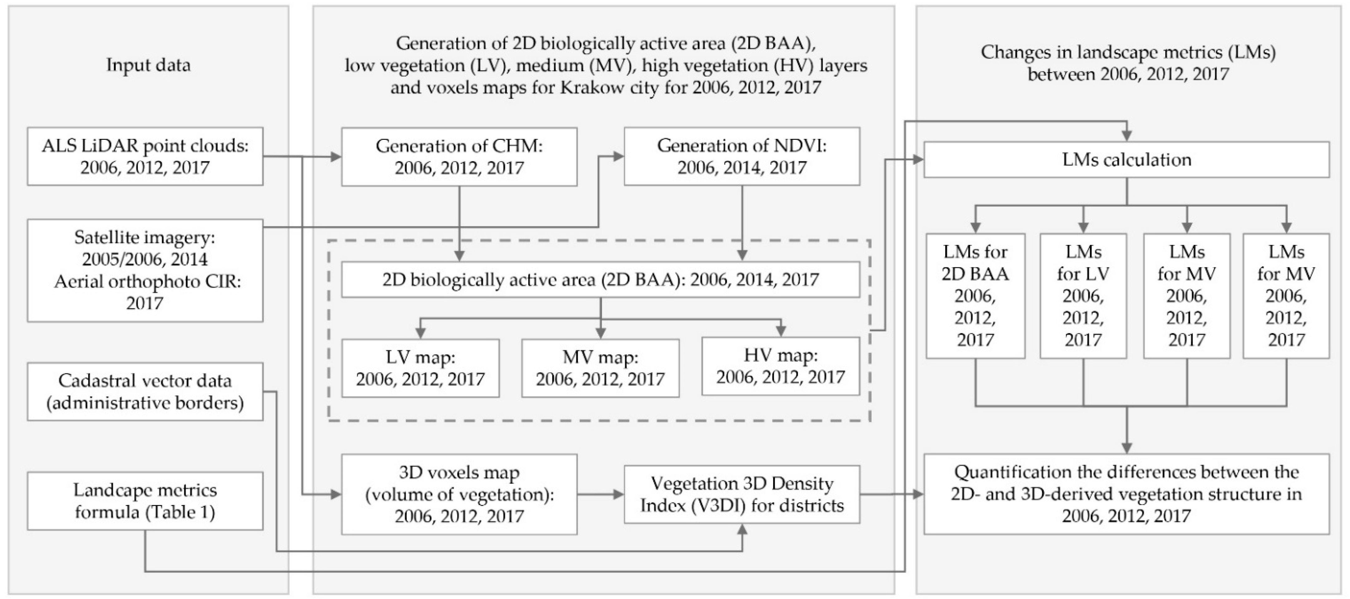
The LM calculations were performed in RStudio with the ‘landscapemetrics’ package “Landscape Metrics for Categorical Map Patterns” [65] based on the vegetation maps produced and described in Section 2.3. The package ’landscapemetrics’ reimplements the most common metrics from the FRAGSTATS software [14] and implements new ones from the current literature on landscape metrics. Because the indicator calculations are conducted on raster spatial maps, the 3D vegetation vector layers created during the GEOBIA classification and exported from eCognition were converted back to a raster format (1.0 m GSD). We calculated the landscape metrics separately for each vegetation layer for 2008, 2012, and 2017, i.e., low vegetation (LV), medium vegetation (MV), high vegetation (HV), and all 2D biologically active areas (2D BAA). The flowchart of the performed analyses is presented in Figure 3.

Figure 3.
Flowchart of analyses (ALS—Airborne Laser Scanning; CHM—Canopy Height Model; CIR—Color-InfraRed; NDVI—Normalized Difference Vegetation Index; 2D BAA—2D biologically active area; LV—low vegetation; MV—medium vegetation; HV—high vegetation; LMs—landscape metrics).
3. Results
3.1. Changes in 2D and 3D Vegetation Cover
The changes in the 2D and 3D perspective vegetation cover and vegetation volume for three periods (2006, 2012, and 2017) were determined by analyzing satellite imagery, aerial orthophotos, and ALS LiDAR data. The following vegetation categories were selected: 2D biologically active area (2D BAA), low vegetation (LV), medium vegetation (MV), and high vegetation (HV). Figure 4 and Figure 5 show the classified land cover maps of vegetation, with a detailed view of the part of Krakow.
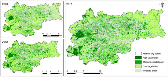
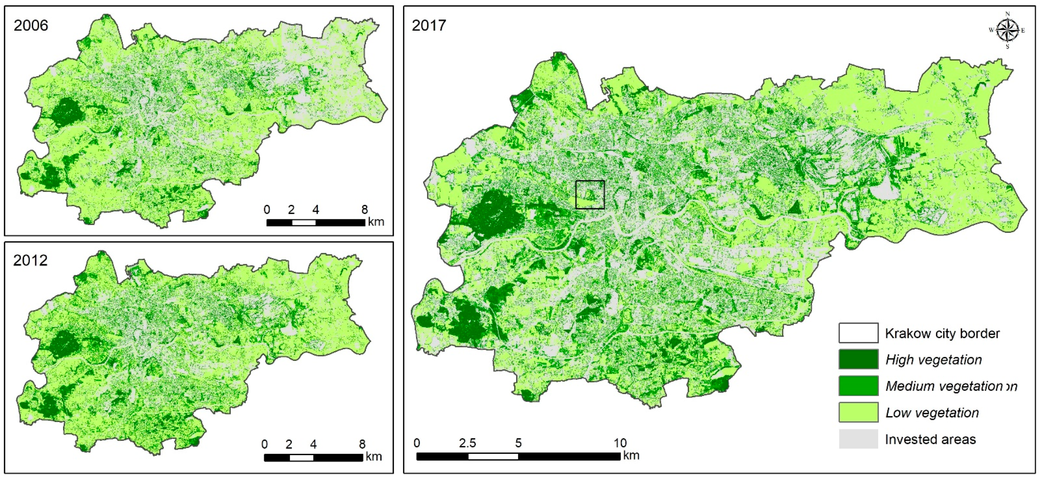
Figure 4.
Results of Krakow vegetation classification for 2006, 2012, and 2017.
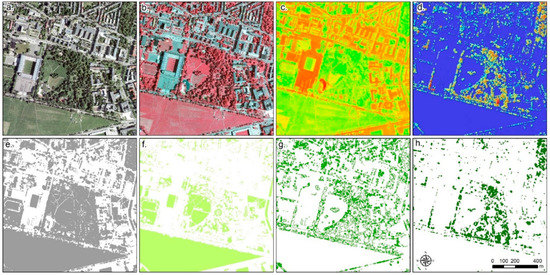
Figure 5.
A detailed view of the part of Krakow in 2017 with different data sources and result layers of 2D/3D vegetation: (a) RGB aerial orthophoto; (b) CIR aerial orthophoto; (c) NDVI; (d) CHM; (e) 2D BAA mask of the urban “green” areas (grey pixels) and non-green (white pixels) areas; and 3D vegetation layers: (f) LV; (g) MV; (h) HV.
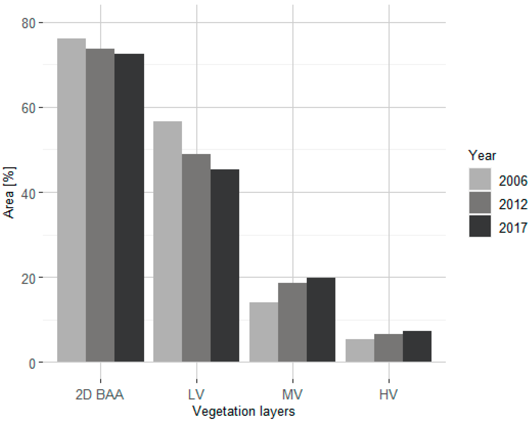
The results show that the total area of 2D BAA for Krakow decreased from 24,872 ha (2006) through 24,110 ha (2012) and continued to 23,655 ha (2017), which is a city-wide decrease in green spaces from 76.1% to 73.8% and 72.4%, respectively. For 3D vegetation, where the relative height was considered: the low vegetation (H < 2.0 m) areas shrank from 56.6% (2006) through 48.8% (2012) to 45.3% (2017). In contrast, medium and high vegetation (H > 2.0 m) increased in the city area, from 19.5% (2006) to 25% (2012) and reaching 27.1% in 2017. Individually, both vegetation classes (MV and HV) increased, as presented in Figure 6. A summary of the area covered by each vegetation class and the percentage area of Krakow in particular years are presented in Table 3.
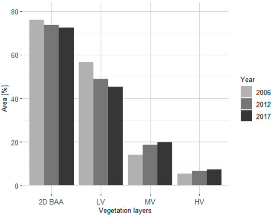
Figure 6.
Changes in vegetation area [%] in Krakow according to year.
Table 3.
Vegetation cover in Krakow for 2006, 2012, and 2017.
3.2. Vegetation Volume and Vegetation 3D Density Index
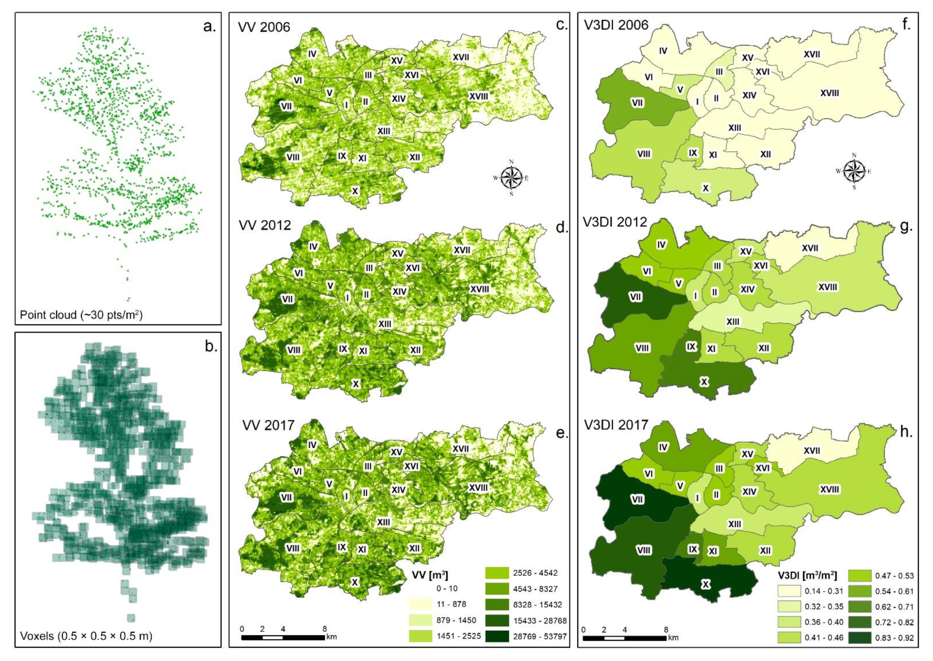
Using the voxel approach, we calculated the vegetation volume (VV) based on the classified ALS LiDAR point cloud. We counted the sum of all voxels (0.5 × 0.5 × 0.5 m) representing the medium and high vegetation classes in the study area, assuming that a single voxel was 0.125 m3. We created raster maps containing the sum of voxels (GSD 0.5 m and 100 m [50]) for Krakow in 2006, 2012, and 2017 (Figure 7). As a result, the total VV in the Krakow city increased in the following years, from about 100 million m3 (2006) through 160 million m3 (2012) and reaching 180 million m3 at the end of the analysis (2017).

Figure 7.
Vegetation volume based on the ALS point cloud (a) converted into 0.5 m × 0.5 m × 0.5 m (x, y, z) voxels (b). Maps of the Vegetation Volume (VV) as the sum volume of voxels in 2006 (c), 2012 (d), and 2017 (e), and the Vegetation 3D Density Index (V3DI) in the Krakow city districts (I-XVIII) in 2006 (f), 2012 (g), and 2017 (h).
In order to compare the changes in the vegetation volume at different levels of detail, we calculated the Vegetation 3D Density Index (V3DI) for all of the city districts (Table 4). The overall value of the V3DI Index for entire Krakow city was increasing over the different timestamps from 0.31 m3/m2 (2006) to 0.48 m3/m2 (2012) and finally reaching 0.56 m3/m2 (2017). The most abundant city districts in terms of vegetation volume, which had the highest V3DI at each analyzed time point, were Zwierzyniec (VII), Swoszowice (X), Dębniki (VIII), and Łagiewniki (IX). In 2006, the Krowodrza (V) city district was characterized by one of the higher V3DI indexes; however, in the following years, it decreased in relation to other districts due to the development of residential and invested zones. The lowest value of V3DI was found for the Wzgórza Krzesławickie (XVII), Podgórze (XIII), and Stare Miasto (I—Old Town) districts (Figure 7).
Table 4.
Vegetation Volume (VV) and Vegetation 3D Density Index (V3DI) calculated for the Krakow districts for 2006, 2012, and 2017.
3.3. Landscape Metrics in Evaluation 2D and 3D Urban Forest Change
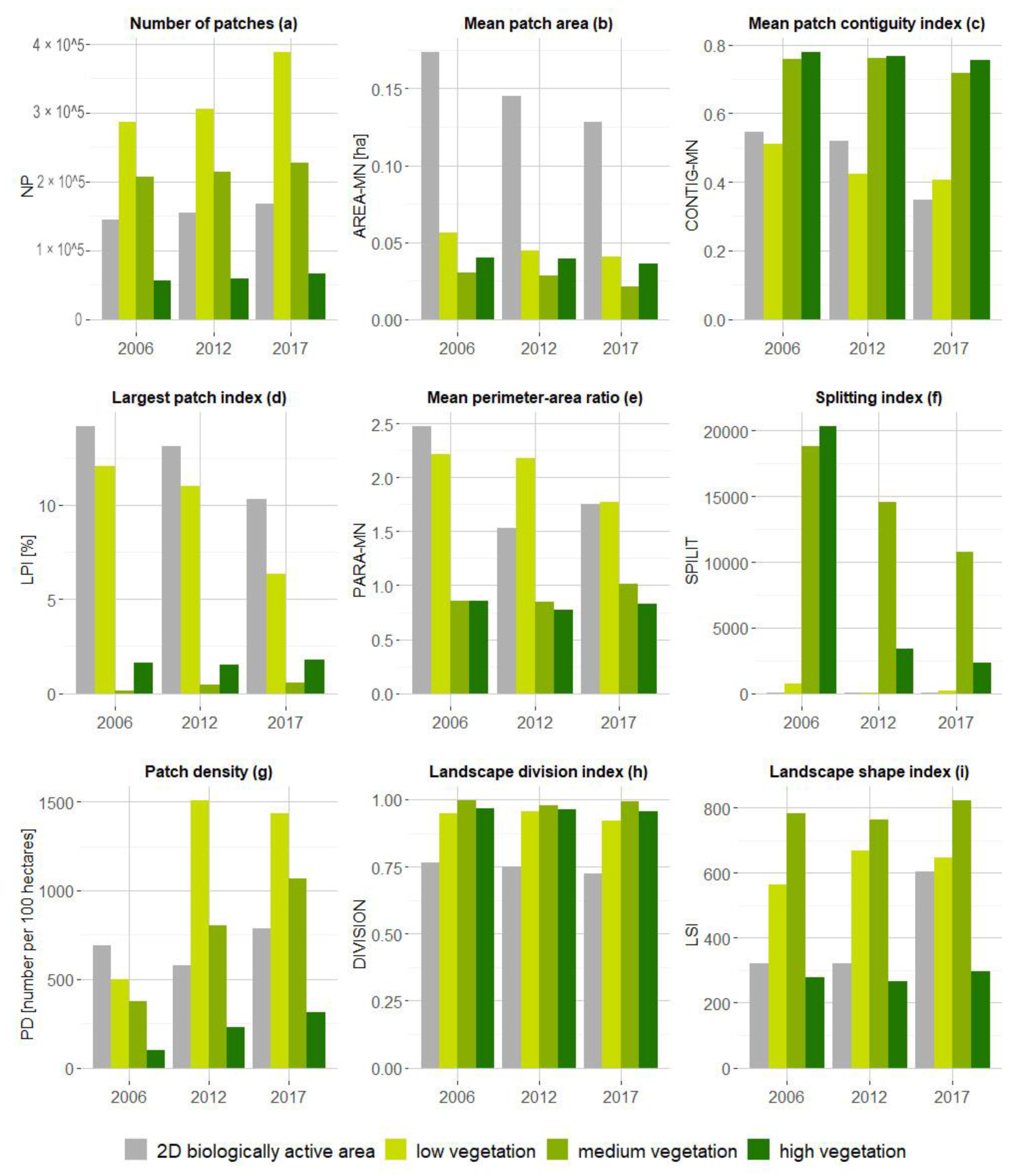
A set of landscape metrics was calculated for the several layers representing vegetation derived from the 2D and 3D analyses to compare the differences between them and thus the impact of the type of vegetation strata on the determination of the fragmentation or connectivity of the landscape. The quantification of the landscape metrics for the 2D BAA and 3D vertical strata—high vegetation, medium vegetation, and low vegetation in specific timestamps (2006, 2012, 2017)—allowed us to describe the spatiotemporal changes occurring in Krakow’s landscape (Figure 8). Table 5 summarizes the values of the calculated LM for each vegetation class.

Figure 8.
Landscape metrics derived from the analysis of the 2D biologically active area (2D BAA; grey bars) and 3D structural layers—low, medium, and high vegetation (LV, MV, and HV; greenish bars) in 2006, 2012, and 2017.
Table 5.
Landscape metrics calculated for Krakow UF for 2006, 2012, and 2017.
The Number of Patches (NP), which describes the fragmentation of a whole class, steadily increased for 2D BAA from 143,991 (2006) through 155,051 (2012) to 167,253 (2017). The NP metrics also increased for all 3D vegetation types (LV, MV, and HV), showing the highest dynamic of changes in the LV class for the last 2012–2017 time interval. The increase in the NP combined with the reduction in 2D BAA (Table 3) is indicative of increased fragmentation, resulting in the division of green spaces into smaller patches, which is often a result of the sprawl of developed areas and the conversion of agriculture into built-up areas.
In all 2D and 3D green space classes for Kraków, the Mean Patch Area (AREA-MN) metric decreased over the years. For the 2D BAA class, the level of this metric was 0.17 ha (2006), 0.15 ha (2012), and 0.13 ha (2017). This shows a decrease in the average vegetation patch area and indicates an increase in the interspersion classes, i.e., the interpenetration of green land cover classes and man-made invested areas. The AREA-MN metric, with very low values close to 0.0 for specific vegetation classes, combined with the total class area, gives an idea of the structure of the patches, which indicates that there are many small objects. The continual reduction of the vegetation class patches area results in a greater openness of the greenery, which may be subject to degradation, increasing the ecological pressure on urban green spaces.
When analyzing the 2D urban greenery, the level of the Mean Patch Contiguity Index (CONTIG-MN) decreased for the 2D BAA layer from 0.55 in 2006 to 0.52 in 2012 and, ultimately, to as low as 0.35 in 2017, approaching a value of 0, indicating a significant reduction in continuity in the 2D vegetation class. Similar values were observed for this indicator calculated for the LV class. In contrast, the 3D MV and HV classes were characterized by a high CONTIG-MN index value, which was closer to 1, taking values of 0.78, 0.77, and 0.76 (HV class). This indicates high contiguity in the 3D vegetation classes. The only decrease in the value of the index suggests that there are no significant changes and that the continuity of these areas is maintained.
The Largest Patch Index (LPI) measured for the 2D BAA shows that there has been a decrease in this ratio from 14.2% (2006) through 13.1% (2012) to 10.3% (2017), similarly to the LV class (from 12.1% to 6.3% between 2006 and 2017). If it is noticeable that the area of the largest greenery patch is decreasing, this may indicate fragmentation. For the HV class, the value of the LPI indicator varied between 1.64% (2006), 1.5% (2012), and 1.77% (2017), eventually exhibiting a small increasing trend, indicating a merging of patches, which shows that the high vegetation is spreading and merging into a larger patch during this growth in the period from 2006–2017.
The Mean Perimeter-Area Ratio (PARA-MN) for the HV class was close to 0 and remained relatively constant (0.86 in 2006, 0.78 in 2012, 0.83 in 2017), indicating a stable geometric shape for this particular vegetation class. However, for the MV class, the PARA-MN metric increased slightly between 2006 and 2017 (from 0.86 to 1.01, respectively), suggesting increasing complexity in this vegetation class. In contrast, in the LV class, as in the 2D vegetation class, the PARA-MN value decreased slightly (2D BAA: 2.48 in 2006 to 1.75 in 2017) while remaining higher than in the 3D vegetation class, suggesting an increased likelihood of fragmentation.
The Splitting Index (SPLIT) for the 3D vegetation classes was decreasing (for the medium and high vegetation: HV—from 20,377 (2006) to 3385 (2012) and 2326 (2017); MV—from 18,782 (2006) to 14,600 (2012) and 10,734 (2017)) while maintaining a high level, so the 3D vegetation showed consistency across classes relative to the 2D BAA class, where the trend was the opposite, and an increase in this index was observed over the last ten years. The increase marks a split in the 2D vegetation class due to the general dynamics of the changes taking place, as observed in 2D space.
The Effective Mesh Size (MESH) metric showed an increase in the HV class from 2.81 (2006) through 7.61 (2012) to 9.17 (2017). Similarly, in the medium vegetation class. The increase in the MESH index indicates the integrity of these land cover types. In the LV class, there were fluctuations. First, the index increased sharply and then decreased, which may suggest intense changes occurring in different directions in this vegetation class over the years. This situation was also influenced by the different phenological phase of the vegetation, classified on satellite images from different months, which may have caused these differences. In the 2D BAA class, the MESH index decreased from 1683 (2006) to 1387 (2012) and 822 (2017), indicating the observed decreasing contiguity, considering all of the vegetation classes in one layer.
Similarly, the aggregation metric is Patch Density (PD), which indicates the number of patches per 100 ha. A high-density value indicates a more significant fragmentation of the landscape. The variation of this metric showed that intense fragmentation occurred in the 3D vegetation between 2006 and 2012 and was not repeated in subsequent years.
The most significant differences were observed during the time interval for the Landscape Division Index (DIVISION)/Connectivity Index (CI) between the 2D and 3D perspectives. The metric’s value calculated for the LV, MV, and HV classes remained almost constant and high. It was close to 1 (CI > 0.9), indicating increased fragmentation. In contrast, in the 2D BAA class, this metric was consistently lower (CI > 0.7), indicating the greater connectivity of these surfaces compared to that in the 3D classes. Furthermore, the low connectivity in the 3D classes changed slightly over the years, showing a decreasing trend between 2006 and 2017, which would suggest an improvement in connectivity.
The Landscape Shape Index (LSI) for both the 2D and 3D vegetation increased between 2006 and 2017, indicating a higher interspersion and that patches are becoming less compact. This is particularly noticeable in the 2D BAA class, where the metric held steady between 2006 and 2012 and then increased sharply, doubling in value in 2017, suggesting significant changes after 2012 related to the intersections of urban greenery by invested areas (roads, buildings, etc.).
Comparing the relevant landscape metrics calculated for the 2D BAA class and the 3D derived strata (LV, MV, and HV), the measures of landscape fragmentation (or connectivity) differed using the two approaches, indicating general patterns. From a 2D perspective, the landscape was perceived to be more connected than in the 3D layers—the 2D BAA indicated a larger core connected zone compared to the 3D layers (Figure 8d). At the same time, the surfaces were more connected in the 2D BAA than in the 3D layers, as indicated by the Connectivity Index (Landscape Division Index), which had lower values for the 2D BAA than for any of the 3D vegetation layers (Figure 8h).
Regarding the patterns in the connectivity of individual 3D vegetation classes, it was observed that the low vegetation was always (2006, 2012, 2017) the best connected, followed by the high vegetation (HV), which was better connected than the medium vegetation (Figure 8h), which was dispersed in the city space.
4. Discussion
The urban forest landscape can be characterized by a complex vegetation structure that varies in two- and three-dimensional spaces. The change detection and fragmentation of the urban green space is most often performed concerning the 2D spatial extent, without taking into account the vertical structure of the vegetation. For this purpose, land cover maps are used—for example, the CORINE Land Cover (EEA) and, more recently, the ESA WorldCover—a global land cover product at a 10 m resolution based on Sentinel-1 and Sentinel-2 ESA satellite data [66]. However, the final values of the landscape metrics may be influenced by the quality of the LULC map classification due to, among other things, the spatial resolution of the satellite imagery and the health condition of the vegetation. For example, an image with a ground resolution of 30 m (e.g., Landsat; NASA, USGS) may contain, in the city area, more than one land cover class, such as partly built-up forest areas, which may affect the calculated indices (so called “mixels”—heterogenous pixels). Another source of information that is used very often is the vegetation map based on NDVI, which maps the presence or absence of greenery, where the green areas are evenly distributed in space [67]. Undeniably, this is a more straightforward approach, but it insufficiently describes the complexity of the urban vegetation, as presented in Figure 5.
In recent years, discussions have begun to expand the understanding of ’3D’ in landscape ecology, as landscape metrics are associated with a universal ’patch-corridor-matrix’ model, which is to reduce the landscape to a two-dimensional mosaic, ignoring the third dimension. Previous studies have identified recommendations to extend the currently functioning set of metrics to include attributes related to topography (height, slope, aspect) [68]. However, so far, 3D landscape metrics have not yet been developed.
Using Airborne Laser Scanning point clouds, we were able to separate the different vertical layers of vegetation (LV, MV, and HV) and calculate the volume of two of those classes (MV and HV). Thus, we created 3D maps of UF and the traditional 2D maps of UF. Then, we were able to estimate the differences that arise in the calculated landscape indices due to the different interpretations—from 2D and 3D perspectives. As a novelty, we were able to show the impact of 2D and 3D analyses on estimating the results of the fragmentation changes in the city of Krakow over ten years (timestamps: 2006, 2012, 2017). The analyses were possible thanks to the availability of ALS LiDAR data, cyclically acquired since 2006 for Krakow and characterized by a similar point cloud density. One of the key challenges in studies using landscape metrics is selecting an optimum number of metrics with appropriate information. As many authors point out, the purpose of the study determines their selection [69,70]. We identified an appropriate set of metrics through the literature review by testing several different ones and then focused on those selected and used in other studies.
Our study showed that when analyzing landscape metrics to estimate the connectivity of urban green spaces, relying only on 2D data (e.g., NDVI) distorts the results, increasing the potential measure of connectivity by not taking into account the vertical structure of vegetation. Meanwhile, the 3D spatial distribution of low, medium, and high vegetation determines the connectivity for a specific group of organisms. In the landscapes of urban areas, for example, trees are significant, as they are practically the only way for specific groups and are extremely important for these species’ connectivity. In addition, an important aspect is the GIS spatiotemporal analyses of landscape metrics, which allow for the examination of changes over the years, showing the trend and dynamics of change, which is not possible with a single observation over time. When describing individual metrics, care should be taken in their interpretation, although they sometimes appear to be a simple method for describing the landscape composition and configuration details. Over the last decade, the expansion of man-made areas in Krakow has decreased the 2D biologically active areas; this is mainly observed for the low vegetation class. On the other hand, a positive observation concerns the area covered by medium and high vegetation, which has increased over the years, indicating an increase in the number of parks, small urban forests, and pocket parks, which will fit in with the concept of the municipality of Krakow for years to come. At the same time, it is worth emphasizing that increasing the cover of urban forests often did not reduce the fragmentation of these areas. Additional confirmation of this thesis is provided by our estimation of the volume of urban forests (in the medium and high vegetation classes), which increased significantly over the years, partly due to shrubs/trees growth but also due to the creation of new green infrastructure in the city. The developed Vegetation 3D Density Index indicated that in each district of the city, the volume of vegetation increased (Table 4), and, overall, on a city-wide scale, the index increased significantly. At the same time, the lowest V3DI values indicate districts where a greenery deficit is observed (mainly the eastern part of the city and the center—Old Town). Our findings show that the development of Krakow, with an ever-increasing population, has led to changes in the landscape, where invested areas taking up low vegetation areas have become more fragmented. Therefore, planning the land for future investments and managing the urban forest resources must be controlled for green space connectivity. Furthermore, future research on Krakow and the landscape could focus on the impact of fragmentation on the quality of the urban environment, the urban heat island effect, or the absorption capacity of pollutants.
5. Conclusions
This study analyzed changes in the landscape of Krakow for 2006, 2012, and 2017 using landscape metrics, comparing the influence of 2D and 3D perspectives on the measures of landscape connectivity. We generated maps based on satellite images (IKONOS-2; QuickBird-2/DigitalGlobe; WorldView-2/MAXAR), CIR orthophotos, and airborne laser scanning point clouds of 2D biologically active areas and 3D structural layers (low, medium, and high vegetation). Using landscape composition, fragmentation, and configuration metrics (NP, AREA-MN, CONTIG-MN, LPI, PARA-MN, SPLIT, MESH, PD, LSI, and DIVISION), it was possible to investigate the intensity of changes in urban greenery and estimate the fragmentation measures for the 2D and 3D layers. In the study area, the landscape metrics indicated a decrease in the areas with low vegetation due to the expansion of developed areas, while the areas with medium and high vegetation increased. Furthermore, the analyses showed that omitting the vertical information of vegetation and basing the analysis only on the 2D layers characterized by planar vegetation distribution leads to an overestimation of the landscape connectivity. In an urban environment, it is essential to understand and map the vertical structure of vegetation due to its complexity and impact on the connectivity of individual organism species.
Author Contributions
Conceptualization, K.Z.-K. and P.W.; methodology, K.Z.-K.; software, K.Z.-K.; validation, K.Z.-K. and P.W.; formal analysis, K.Z.-K.; investigation, K.Z.-K.; resources, P.W.; data curation, K.Z.-K. and P.W.; writing—original draft preparation, K.Z.-K.; writing—review and editing, K.Z.-K. and P.W.; visualization, K.Z.-K.; supervision, P.W. All authors have read and agreed to the published version of the manuscript.
Funding
This research was supported by the Ministry of Education and Science of the Republic of Poland.
Institutional Review Board Statement
Not applicable.
Informed Consent Statement
Not applicable.
Data Availability Statement
Publicly available ALS LiDAR datasets were analyzed in this study and can be downloaded here: https://www.geoportal.gov.pl/dane/dane-pomiarowe-lidar. The VHRS imagery (MAXAR) are not publicly available due to license limitations.
Acknowledgments
We thank the Municipality of Krakow, the Spatial Planning Office, and the Central Office of Geodesy and Cartography in Poland (GUGiK) for providing the open LiDAR data and aerial orthophotos and the ProGea Consulting Company for providing the satellite imagery for the purpose of this research.
Conflicts of Interest
The authors declare no conflict of interest.
References
- Andersson, E. Urban Landscapes and Sustainable Cities. Ecol. Soc. 2006, 11, 34. [Google Scholar] [CrossRef]
- Fan, X.; Yu, H.; Tiando, D.S.; Rong, Y.; Luo, W.; Eme, C.; Ou, S.; Li, J.; Liang, Z. Impacts of Human Activities on Ecosystem Service Value in Arid and Semi-Arid Ecological Regions of China. Int. J. Environ. Res. Public Health 2021, 18, 11121. [Google Scholar] [CrossRef] [PubMed]
- Solon, J. Spatial context of urbanization: Landscape pattern and changes between 1950 and 1990 in the Warsaw metropolitan area, Poland. Landsc. Urban Plan. 2009, 93, 250–261. [Google Scholar] [CrossRef] [Green Version]
- Liu, Z.; He, C.; Wu, J. The Relationship between Habitat Loss and Fragmentation during Urbanization: An Empirical Evaluation from 16 World Cities. PLoS ONE 2016, 11, e0154613. [Google Scholar] [CrossRef]
- Endreny, T.A. Strategically growing the urban forest will improve our world. Nat. Commun. 2018, 9, 1160. [Google Scholar] [CrossRef] [PubMed] [Green Version]
- Colding, J.; Gren, A.; Barthel, S. The Incremental Demise of Urban Green Spaces. Land 2020, 9, 162. [Google Scholar] [CrossRef]
- Forman, R.T. Landscape Ecology; Wiley: New York, NY, USA, 1986; ISBN 978-0-471-87037-1. [Google Scholar]
- Frazier, A.E.; Kedron, P. Landscape Metrics: Past Progress and Future Directions. Curr. Landsc. Ecol. Rep. 2017, 2, 63–72. [Google Scholar] [CrossRef] [Green Version]
- Gardner, R.H.; Mime, B.T.; Turner, M.G.; O’neill, R.V. Neutral models for the analysis of broad-scale landscape pattern. Landsc. Ecol. 1987, 1, 19–28. [Google Scholar] [CrossRef]
- O’Neill, R.V.; Krummel, J.R.; Gardner, R.H.; Sugihara, G.; Jackson, B.; DeAngelis, D.L.; Milne, B.T.; Turner, M.G.; Zygmunt, B.; Christensen, S.W.; et al. Indices of landscape pattern. Landsc. Ecol. 1988, 1, 153–162. [Google Scholar] [CrossRef]
- Ricotta, C. From theoretical ecology to statistical physics and back: Self-similar landscape metrics as a synthesis of ecological diversity and geometrical complexity. Ecol. Model. 2000, 125, 245–253. [Google Scholar] [CrossRef]
- Parrott, L.; Proulx, R.; Thibert-Plante, X. Three-dimensional metrics for the analysis of spatiotemporal data in ecology. Ecol. Inform. 2008, 3, 343–353. [Google Scholar] [CrossRef]
- Gustafson, E.J. How has the state-of-the-art for quantification of landscape pattern advanced in the twenty-first century? Landsc. Ecol. 2018, 34, 2065–2072. [Google Scholar] [CrossRef]
- McGarigal, K.; Marks, B.J. FRAGSTATS: Spatial pattern analysis program for quantifying landscape structure. In General Technical Report; PNW-GTR-351; U.S. Department of Agriculture, Forest Service: Washington, DC, USA; Pacific Northwest Research Station: Portland, OR, USA, 1995; p. 122. [Google Scholar] [CrossRef]
- Vogt, P.; Riitters, K. GuidosToolbox: Universal digital image object analysis. Eur. J. Remote Sens. 2017, 50, 352–361. [Google Scholar] [CrossRef]
- Hesselbarth, M.H.K.; Sciaini, M.; With, K.A.; Wiegand, K.; Nowosad, J. landscapemetrics: An open-source R tool to calculate landscape metrics. Ecography 2019, 42, 1648–1657. [Google Scholar] [CrossRef] [Green Version]
- Kaminski, A.; Bauer, D.M.; Bell, K.P.; Loftin, C.S.; Nelson, E.J. Using landscape metrics to characterize towns along an urban-rural gradient. Landsc. Ecol. 2021, 36, 2937–2956. [Google Scholar] [CrossRef]
- Long, Y.; Gu, Y.; Han, H. Spatiotemporal heterogeneity of urban planning implementation effectiveness: Evidence from five urban master plans of Beijing. Landsc. Urban Plan. 2012, 108, 103–111. [Google Scholar] [CrossRef]
- Estoque, R.C.; Murayama, Y. Landscape pattern and ecosystem service value changes: Implications for environmental sustainability planning for the rapidly urbanizing summer capital of the Philippines. Landsc. Urban Plan. 2013, 116, 60–72. [Google Scholar] [CrossRef]
- He, C.; Wei, A.; Shi, P.; Zhang, Q.; Zhao, Y. Detecting land-use/land-cover change in rural–urban fringe areas using extended change-vector analysis. Int. J. Appl. Earth Obs. Geoinf. 2011, 13, 572–585. [Google Scholar] [CrossRef]
- Smiraglia, D.; Ceccarelli, T.; Bajocco, S.; Perini, L.; Salvati, L. Unraveling Landscape Complexity: Land Use/Land Cover Changes and Landscape Pattern Dynamics (1954–2008) in Contrasting Peri-Urban and Agro-Forest Regions of Northern Italy. Environ. Manag. 2015, 56, 916–932. [Google Scholar] [CrossRef]
- Kumar, M.; Denis, D.M.; Singh, S.K.; Szabó, S.; Suryavanshi, S. Landscape metrics for assessment of land cover change and fragmentation of a heterogeneous watershed. Remote Sens. Appl. Soc. Environ. 2018, 10, 224–233. [Google Scholar] [CrossRef] [Green Version]
- Cyriac, S.; Firoz, C.M. A Bibliometric Review of Publication Trends in the Application of Landscape Metrics in Urban and Regional Planning. Pap. Appl. Geogr. 2022, 1–18. [Google Scholar] [CrossRef]
- Fu, G.; Wang, W.; Li, J.; Xiao, N.; Qi, Y. Prediction and Selection of Appropriate Landscape Metrics and Optimal Scale Ranges Based on Multi-Scale Interaction Analysis. Land 2021, 10, 1192. [Google Scholar] [CrossRef]
- Angel, S.; Parent, J.; Civco, D.L. The fragmentation of urban landscapes: Global evidence of a key attribute of the spatial structure of cities, 1990–2000. Environ. Urban. 2012, 24, 249–283. [Google Scholar] [CrossRef] [Green Version]
- Lin, Y.; An, W.; Gan, M.; Shahtahmassebi, A.; Ye, Z.; Huang, L.; Zhu, C.; Huang, L.; Zhang, J.; Wang, K. Spatial Grain Effects of Urban Green Space Cover Maps on Assessing Habitat Fragmentation and Connectivity. Land 2021, 10, 1065. [Google Scholar] [CrossRef]
- Vogt, P.; Ferrari, J.R.; Lookingbill, T.R.; Gardner, R.H.; Riitters, K.H.; Ostapowicz, K. Mapping functional connectivity. Ecol. Indic. 2009, 9, 64–71. [Google Scholar] [CrossRef]
- Sinha, P.; Kumar, L.; Reid, N. Rank-Based Methods for Selection of Landscape Metrics for Land Cover Pattern Change Detection. Remote Sens. 2016, 8, 107. [Google Scholar] [CrossRef] [Green Version]
- Cushman, S.A.; McGarigal, K. Metrics and Models for Quantifying Ecological Resilience at Landscape Scales. Front. Ecol. Evol. 2019, 7, 440. [Google Scholar] [CrossRef] [Green Version]
- Chen, Z. The Application of Airborne Lidar Data in the Modelling of 3D Urban Landscape Ecology; Cambridge Scholars Publishing: Newcastle upon Tyne, UK, 2017; ISBN 1-4438-9986-0. [Google Scholar]
- Jaeger, J.A.G. Landscape division, splitting index, and effective mesh size: New measures of landscape fragmentation. Landsc. Ecol. 2000, 15, 115–130. [Google Scholar] [CrossRef]
- Tian, Y.; Jim, C.Y.; Tao, Y.; Shi, T. Landscape ecological assessment of green space fragmentation in Hong Kong. Urban For. Urban Green. 2011, 10, 79–86. [Google Scholar] [CrossRef]
- Ciesielski, M.; Stereńczak, K. Accuracy of determining specific parameters of the urban forest using remote sensing. IFor. Biogeosci. For. 2019, 12, 498–510. [Google Scholar] [CrossRef] [Green Version]
- Wahyudi, A.; Liu, Y.; Corcoran, J. Combining Landsat and landscape metrics to analyse large-scale urban land cover change: A case study in the Jakarta Metropolitan Area. J. Spat. Sci. 2019, 64, 515–534. [Google Scholar] [CrossRef]
- Qing, L.; Petrosian, H.A.; Fatholahi, S.N.; Chapman, M.A.; Li, J. Quantifying urban expansion using Landsat images and landscape metrics: A case study of the Halton Region, Ontario. Geomatica 2020, 74, 220–237. [Google Scholar] [CrossRef]
- Nasehi, S.; Namin, A.I. Assessment of urban green space fragmentation using landscape metrics (case study: District 2, Tehran city). Model. Earth Syst. Environ. 2020, 6, 2405–2414. [Google Scholar] [CrossRef]
- Fichera, C.R.; Modica, G.; Pollino, M. Land Cover classification and change-detection analysis using multi-temporal remote sensed imagery and landscape metrics. Eur. J. Remote Sens. 2012, 45, 1–18. [Google Scholar] [CrossRef]
- Wężyk, P.; Hawryło, P.; Szostak, M.; Pierzchalski, M.; De Kok, R. Using Geobia and Data Fusion Approach for Land use and Land Cover Mapping. Quaest. Geogr. 2016, 35, 93–104. [Google Scholar] [CrossRef] [Green Version]
- Zięba-Kulawik, K.; Wężyk, P. Detection of high vegetation cover change in Krakow in 2016-2017 based on GEOBIA approach of RapidEye (Planet) satellite imagery. In Współczesne Problemy i Kierunki Badawcze w Geografii; Contemporary Problems and Research Directions in Geography; Instytut Geografii i Gospodarki Przestrzennej UJ.: Kraków, Poland, 2019; Volume 7, pp. 199–226. [Google Scholar]
- Arora, A.; Pandey, M.; Mishra, V.N.; Kumar, R.; Rai, P.K.; Costache, R.; Punia, M.; Di, L. Comparative evaluation of geospatial scenario-based land change simulation models using landscape metrics. Ecol. Indic. 2021, 128, 107810. [Google Scholar] [CrossRef]
- Sertel, E.; Topaloğlu, R.H.; Bahşi, K.; Varol, B.; Musaoğlu, N. Production of a Land Cover/Land Use (LC/LU) Map of Izmir Metropolitan City by Using High-Resolution Images. In Environmental Science and Engineering; Springer: Cham, Switzerland, 2021; pp. 1837–1846. [Google Scholar] [CrossRef]
- Sertel, E.; Topaloğlu, R.H.; Şallı, B.; Algan, I.Y.; Aksu, G.A. Comparison of Landscape Metrics for Three Different Level Land Cover/Land Use Maps. ISPRS Int. J. Geo-Inf. 2018, 7, 408. [Google Scholar] [CrossRef] [Green Version]
- Wezyk, P.; Tompalski, P.; Szostak, M.; Glista, M.; Pierzchalski, M. Describing the selected canopy layer parameters of the Scots pine stands using ALS data. In Proceedings of the 8th International Conference on LiDAR Applications In forest Assessment and Inventory, Heriot-Watt University, Edinburgh, UK, 17–19 September 2008; pp. 636–645. [Google Scholar]
- Matasci, G.; Coops, N.C.; Williams, D.A.R.; Page, N. Mapping tree canopies in urban environments using airborne laser scanning (ALS): A Vancouver case study. For. Ecosyst. 2018, 5, 31. [Google Scholar] [CrossRef] [Green Version]
- Koma, Z.; Zlinszky, A.; Bekő, L.; Burai, P.; Seijmonsbergen, A.C.; Kissling, W.D. Quantifying 3D vegetation structure in wetlands using differently measured airborne laser scanning data. Ecol. Indic. 2021, 127, 107752. [Google Scholar] [CrossRef]
- Plowright, A.A.; Coops, N.C.; Eskelson, B.N.I.; Sheppard, S.R.J.; Aven, N.W. Assessing urban tree condition using airborne light detection and ranging. Urban For. Urban Green. 2016, 19, 140–150. [Google Scholar] [CrossRef]
- Bajorek-Zydroń, K.; Wężyk, P. Atlas Pokrycia Terenu i Przewietrzania Krakowa; Urząd Miasta Krakowa, Wydział Kształtowania Środowiska: Kraków, Poland, 2016; ISBN 978-83-918196-5-4. [Google Scholar]
- Hancock, S.; Anderson, K.; Disney, M.; Gaston, K.J. Measurement of fine-spatial-resolution 3D vegetation structure with airborne waveform lidar: Calibration and validation with voxelised terrestrial lidar. Remote Sens. Environ. 2017, 188, 37–50. [Google Scholar] [CrossRef] [Green Version]
- Anderson, K.; Hancock, S.; Casalegno, S.; Griffiths, A.; Griffiths, D.; Sargent, F.; McCallum, J.; Cox, D.T.C.; Gaston, K.J. Visualising the urban green volume: Exploring LiDAR voxels with tangible technologies and virtual models. Landsc. Urban Plan. 2018, 178, 248–260. [Google Scholar] [CrossRef]
- Zięba-Kulawik, K.; Skoczylas, K.; Wężyk, P.; Teller, J.; Mustafa, A.; Omrani, H. Monitoring of urban forests using 3D spatial indices based on LiDAR point clouds and voxel approach. Urban For. Urban Green. 2021, 65, 127324. [Google Scholar] [CrossRef]
- Kedron, P.; Zhao, Y.; Frazier, A.E. Three dimensional (3D) spatial metrics for objects. Landsc. Ecol. 2019, 34, 2123–2132. [Google Scholar] [CrossRef]
- Frazier, A. Landscape Metrics. In The Geographic Information Science & Technology Body of Knowledge; Association of American Geographers: Corvallis, OR, USA, 2019. [Google Scholar] [CrossRef]
- Casalegno, S.; Anderson, K.; Cox, D.T.C.; Hancock, S.; Gaston, K.J. Ecological connectivity in the three-dimensional urban green volume using waveform airborne lidar. Sci. Rep. 2017, 7, 45571. [Google Scholar] [CrossRef] [Green Version]
- Babiarz, P.; Dziedzic, A.; Kłósek, M.; Łacic, M.; Piwowarczyk, M.; Rudnik, K.; Tutaj, J.; Ziomek-Pożoga, A. Statistical Yearbook of Kraków; Statistical Office in Kraków: Krakow, Poland, 2021.
- Zachariasz, A. Development of the System of the Green Areas of Krakow from The Nineteenth Century to The Present, in The Context of Model Solutions. IOP Conf. Ser. Mater. Sci. Eng. 2019, 471, 112097. [Google Scholar] [CrossRef]
- Jędrychowski, I. Airborne laser scanning of Cracow/Lotnicze skanowanie laserowe Krakowa. Arch. Fotogram. Kartogr. Teledetekcji 2007, 17, 339–345. [Google Scholar]
- Wężyk, P. Podręcznik dla Uczestników Szkoleń z Wykorzystania Produktów LiDAR; Wężyk, P., Ed.; Główny Urząd Geodezji i Kartografii: Warszawa, Poland, 2014; ISBN 978-83-254-2090-1. [Google Scholar]
- Tucker, C.J. Red and photographic infrared linear combinations for monitoring vegetation. Remote Sens. Environ. 1979, 8, 127–150. [Google Scholar] [CrossRef] [Green Version]
- Liang, S. Quantitative Remote Sensing of Land Surfaces; John Wiley & Sons, Inc.: Hoboken, NJ, USA, 2004. [Google Scholar]
- McGaughey, R.J. FUSION/LDV: Software for LIDAR Data Analysis and Visualization; USDA Forest Service: Seattle, WA, USA; Pacific Northwest Research Station: Corvallis, OR, USA, 2015.
- Baatz, M.; Schäpe, A. Multiresolution Segmentation-an optimization approach for high quality multi-scale image segmentation. In XII Angewandte Geographische Informationsverarbeitung; Wichmann-Verlag: Heidelberg, Germany, 2000. [Google Scholar]
- Roussel, J.-R.; Auty, D.; De Boissieu, F.; Meador, A.S.; Jean-François, B.; Demetrios, G.; Steinmeier, L.; Adaszewski, S. Package “lidR” Airborne LiDAR Data Manipulation and Visualization for Forestry Applications; 2022. Available online: https://cran.r-project.org/web/packages/lidR/index.html (accessed on 1 May 2022).
- Lausch, A.; Blaschke, T.; Haase, D.; Herzog, F.; Syrbe, R.-U.; Tischendorf, L.; Walz, U. Understanding and quantifying landscape structure—A review on relevant process characteristics, data models and landscape metrics. Ecol. Model. 2015, 295, 31–41. [Google Scholar] [CrossRef]
- Herold, M.; Couclelis, H.; Clarke, K.C. The role of spatial metrics in the analysis and modeling of urban land use change. Comput. Environ. Urban. Syst. 2005, 29, 369–399. [Google Scholar] [CrossRef]
- Hesselbarth, M.H.K.; Sciaini, M.; Nowosad, J.; Hanss, S.; Graham, L.J.; Hollister, J.; With, K.A.; Prive, F.; Strimas-Mackey, M. landscapemetrics: Landscape Metrics for Categorical Map Patterns; 2021. Available online: https://cran.r-project.org/web/packages/landscapemetrics (accessed on 1 May 2022).
- European Space Agency WorldCover|WORLDCOVER. Available online: https://esa-worldcover.org/en (accessed on 27 March 2022).
- Muratet, A.; Lorrillière, R.; Clergeau, P.; Fontaine, C. Evaluation of landscape connectivity at community level using satellite-derived NDVI. Landsc. Ecol. 2012, 28, 95–105. [Google Scholar] [CrossRef]
- Stupariu, M.S.; Pàtru-Stupariu, I.G.; Cuculici, R. Geometric approaches to computing 3D-landscape metrics. Landsc. Online 2010, 24, 1–12. [Google Scholar] [CrossRef]
- Uuemaa, E.; Roosaare, J.; Oja, T.; Mander, Ü. Analysing the spatial structure of the Estonian landscapes: Which landscape metrics are the most suitable for comparing different landscapes? Est. J. Ecol. 2011, 60, 70–80. [Google Scholar] [CrossRef] [Green Version]
- Cushman, S.A.; McGarigal, K.; Neel, M.C. Parsimony in landscape metrics: Strength, universality, and consistency. Ecol. Indic. 2008, 8, 691–703. [Google Scholar] [CrossRef]

Publisher’s Note: MDPI stays neutral with regard to jurisdictional claims in published maps and institutional affiliations. |
© 2022 by the authors. Licensee MDPI, Basel, Switzerland. This article is an open access article distributed under the terms and conditions of the Creative Commons Attribution (CC BY) license (https://creativecommons.org/licenses/by/4.0/).