1. Introduction
Plant health and productivity in agricultural settings have vital roles in ecosystem health and economic benefits. Changes in precipitation amounts and intensities concurrent with increasing air temperatures are a common threat to the agricultural fields arising from climate change [
1]. Food security is becoming a major issue worldwide [
2], and land suitability for crop growth might shift due to climatic change [
3]. Environmental changes, such as drought or soil chemistry modifications, can be reflected in changes in the physical appearance of plants [
4,
5]. These changes can provide rapid information about plant health, indicating the need for further action to secure plant productivity. The best way to prepare and to develop mitigating measures from climate change-related negative impacts is to monitor changes of the complex plant–soil–water system to the varying environmental conditions.
Monitoring of plant health may consist of observing belowground environmental conditions such as soil water content (SWC) or temperature, and aboveground plant conditions such as leaf greenness or canopy density. Spectral properties of plants, such as the Normalized Vegetation Index (NDVI) or the Photochemical Reflectance Index (PRI), can be used to monitor plant health and soil–plant–water relations. NDVI might be used to retrieve data on plant greenness and density [
6]. It can also be used as a proxy for annual aboveground net primary production (NPP), commonly integrated over the entire growing season [
7]. Plant stress induced by soil water- or nutrient-related changes can be studied by measuring PRI [
8,
9]. The fraction of absorbed photosynthetically active radiation (fAPAR) values can be used for estimating the leaf area index (LAI), providing information on canopy structure. Leaf surface area plays an important role in the global cycles of carbon, nitrogen, and water [
10]. The LAI has been widely used as an indicator of plant health. The chlorophyll content is highly affected by leaf nitrogen concentrations as leaves are an important part of the photosynthetic activities in many aspects [
11]. The information on plant LAI is not only a vital part of understanding a given ecosystem, but also an important input for crop yield or climate models [
12].
Soil physical and chemical characteristics can greatly influence plant growth and development. In agricultural lands, the spatial variations of topography, physical, and chemical characteristics of soils result in varying crop and fruit yield, which for vineyards can be crucial for wine quality and volume [
13]. While spatial heterogeneity due to erosion or topographic conditions changes the soil characteristics the plants are growing in, the plants also change soil conditions as they grow [
14]. A healthy plant takes up a higher amount of water and nutrients from the soil during its development compared to an ailing plant with lower biomass or a less dense root structure.
Slope position can greatly affect plant growth, mainly due to differences in soil physical and chemical properties resulting from soil erosion processes, or radiation exposure due to elevation changes. SWC can vary at a different part of the slopes as soil hydraulic conditions change [
15]. Soil properties, especially organic matter content, can explain a significant portion of crop yield or fruit production differences at a given topographical land feature [
16]. Due to soil redistribution processes, the upper portions of the slopes are often more degraded, while at lower parts, soil depositions occur. Consequently, NPP can also decrease towards the upper portion of a slope, as soil water content or nitrogen availability might decrease [
17]. Soil deterioration and land degradation are major threats to crop production; therefore, to keep agricultural lands sustainable, conservational soil management practices should be implemented whenever possible [
18]. However, to develop proper conservation strategies, some background knowledge on land resource use and monitoring activities is necessary.
While the topography of a given area influences the spatial distribution of soil properties, such as organic matter content [
19,
20], the land use type is another major factor controlling soil chemistry [
21]. Plants in different land use types have varying nutrition and water needs. For example, compared to grass, grapes need 30% less water, while maize needs approximately 10% more [
22]. Therefore, the same amount of precipitation might be right for grapes but can cause water stress for maize in rainfed lands. Plants with deeper root structures promote preferential water flow, enabling rainwater to enter the deeper part of the soil matrix, which in turn is available for plant uptake during drought conditions [
23,
24]. Soil water content is one of the major factors affecting soil ecosystem health, which is highly dependent on the water-holding capacity (WHC) of a given soil. WHC is an important soil physical parameter for plant available water in drought-prone areas, and especially, with increasing soil temperatures due to climatic changes, the evaporation rates can also be expected to increase. Sandy soils have lower, while clayey soils have higher water-holding capacities, however the soil chemistry such as organic matter content [
25] or the soil management system used [
26,
27] can also affect the soils’ WHC. Therefore, improving plant available WHC of soils is an important aspect of mitigating climate change-related negative effects.
Satellite images have become extensively useful tools to access data on terrestrial information, such as crop yield estimates or plant health. Sentinel-2 products with free accessibility of the complete archive of 10–20 m resolution images along with the computing ability of the Google Earth Engine [
28] enable researchers to better assess remote sensing applications for ground measurements. Sentinel-2 data have been successfully used for crop yield estimation [
29,
30]. Furthermore, NDVI or canopy data derived from satellite imagery can be important crop model input parameters, resulting in a better estimation of crop or fruit yield [
31].
To better understand the soil–plant–water relations under varying land use types and environmental conditions, field measurements can offer valuable information. While atmospheric conditions such as ozone or water vapor content can influence sensor reflectance [
32], optical satellite imagery is dependent on cloud-free views [
33]. Therefore, field observations supplemented with satellite imagery data provide a more accurate assessment of a given study site.
The aim of the present study was to investigate the relationship between soil parameters (soil chemistry, water content, and temperature) and plant reflectance using handheld sensor sets. We also analyzed how slope position affects plant health, as indicated by differences in NDVI, PRI, and fAPAR. Furthermore, data from Sentinel-2 satellite imagery provided an opportunity to further expand the information from our field measurements, affording a more comprehensive picture of the study sites.
2. Materials and Methods
2.1. Site Description
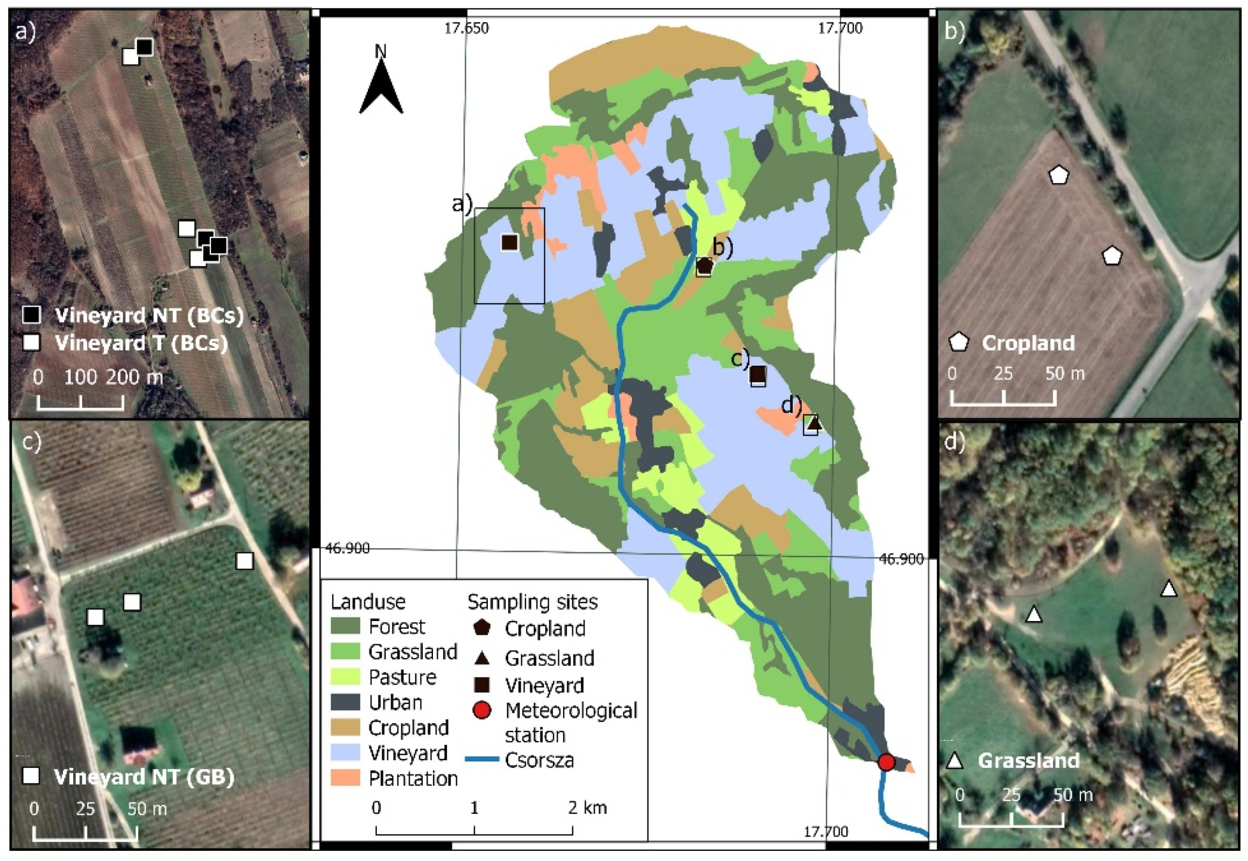
The study sites are located in a small agricultural catchment of the Csorsza stream, which feeds Lake Balaton in Hungary. The total area of the catchment is 21 km2.
The present experiment was carried out in 2021 during the vegetation period (30 June–9 September). Three main land use types with a total of five slopes were selected for the study, with a total of fourteen measuring points. The exact locations of the study sites and points are shown in
Figure 1. The land use types and slope inclinations are the following: cropland with 0–5% slope, two vineyards of BCs (abbreviation is based on location, Balatoncsicsó) and GB (abbreviation is based on location, Gergely Vineyard) with 8–10% and 12–18% slope, respectively, and grassland with 5–10% slope. The soils at the investigated land use sites are Cambisols and Calcisols, according to WRB [
34].
From the five investigated slopes, three of them were vineyard slopes, each with three or four measurement points (upper, lower, and a middle point regarding its position on the slope gradient;
Figure 1a,c). The fourth was a cropland and the fifth was a grassland slope having 2-2 measuring points (one upper and one lower slope position;
Figure 1b,d).
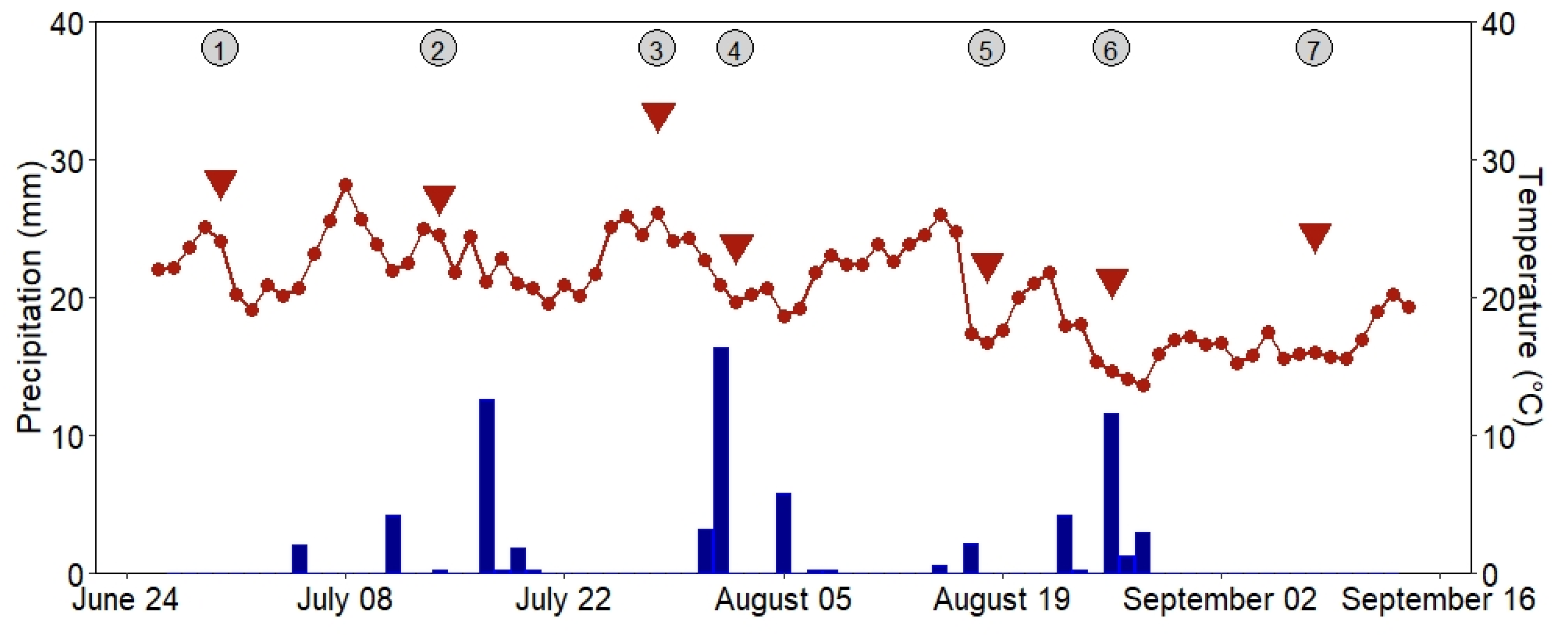
Meteorological data were collected from the meteorological station located at the catchment outlet (
Figure 1). The daily cumulative precipitation and average air and midday temperatures are shown in
Figure 2. The midday data represent the average temperature when field measurements were conducted, i.e., the points in
Figure 2 were based on measurements from 10:00 to 14:00.
A crop rotation system was applied on the field, with maize (Zea mays L.) sown in 2021. At the BCs vineyard, the grape variety is called Riesling (Vitis vinifera L.), while at the GB vineyard, Furmint (Vitis vinifera L.) is grown, and both are white wine grape varieties. The GB vineyard is currently planted with grass inter-rows between the rows, with no tillage. At the BCs site, we investigated plots with grass inter-rows (NT), as well as plots with tilled soil management (T) performed between rows. In 2021, the tilled site had red clover (Trifolium pretense L.) and rye (Secale cereal L.) sown between the rows. The grassland normally has occasional mowing events performed, which in 2021 was once in early July.
2.2. Plant Measurements/Ground Validation Samples
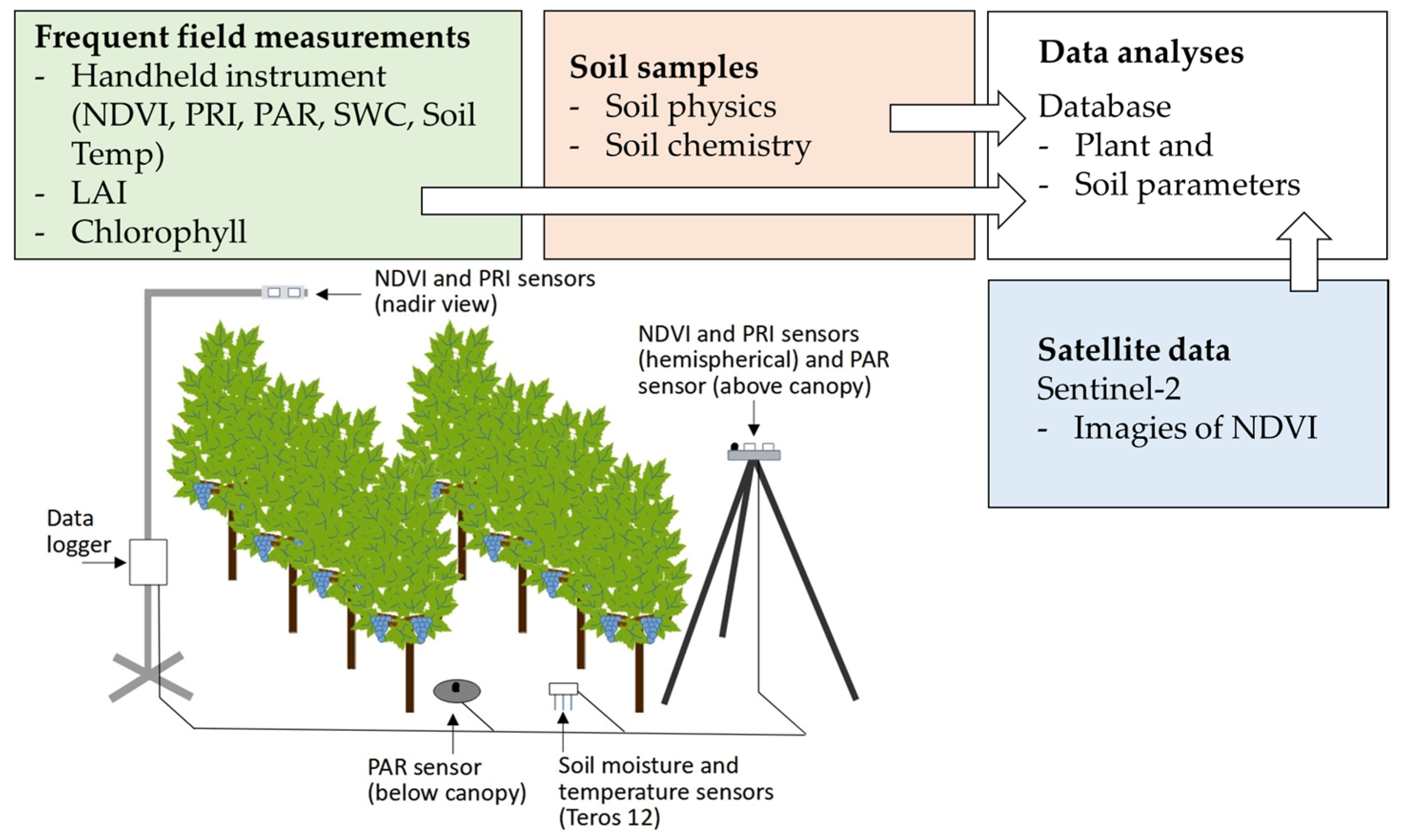
In 2021, field measurements were collected on 7 occasions in the different land use types using a handheld sensor set. This sensor set setup is shown in
Figure 3 and included PRI, NDVI, photochemically active radiation (PAR; METER Group, Pullman, WA, USA), and soil water and temperature sensors (TEROS 12; METER Group).
From the measured PAR values, we calculated the fraction of the absorbed PAR as a difference of the hemispherical and below-canopy radiation flux over the above-canopy radiation flux [
35]. Photon flux values are presented in µmol m
−2 s
−1. At the same time as the PAR measurements, spectral reflectance sensors of PRI and NDVI were measuring 532 and 570 nm and 630 and 800 nm spectral irradiance, respectively.
The PRI values were calculated based on Gamon [
36] using the following equation:
where
Pr represents the field stop lens sensor for reflected radiation from the canopy, while
Pi is the hemispherical sensor for incident radiation values. The uncorrected reflectance values (
Pr/
Pi) were calculated for each waveband (532 and 570 nm) and used to calculate uncorrected PRI.
The NDVI values were calculated based on radiance [
36,
37] using the following equation:
where
Nr represents the field stop lens sensor for reflected radiation from the canopy, while
Ni is the hemispherical sensor for incident radiation values. The uncorrected reflectance values (
Nr/
Ni) were calculated for each waveband (630 and 800 nm) and used to calculate uncorrected NDVI.
While PAR sensors were placed below the canopy, the NDVI and PRI sensors were set into nadir view 2.5 m aboveground. All hemispheric data were collected from nearby immobile stations.
Along with the spectral reflectance sensors, we also used two soil water content and temperature sensors to further analyze the connections between soil water and plant relations. These sensors measured the volumetric water contents of the top 12 cm of the soils.
Concurrent with the handheld sensor set measurements, we determined the leaf area index (LAI) of all three plant types using an AccuPAR LP 80 instrument, which computes the LAI from above- and below-canopy readings of PAR and the leaf angle distribution parameter. Chlorophyll content of the grapevine leaves at the veraison stage was also measured to increase our understanding of the soil–plant–water interactions. We used an Apogee MC-100 instrument, where the values were provided in chlorophyll content index (CCI) for general measurements. The instrument calculates the chlorophyll content from the ratio of optical transmission at 931 nm (NIR wavelength) to the optical transmission at 653 nm (red wavelength). Due to the extreme drought conditions during the measurement time, both the grassland and maize dried out, and therefore measurements were not conducted at these sites.
Most measurements were reduced to 5 values (PRI, PAR, NDVI) or 10 values (SWC, soil temperature, and chlorophyll) per sampling site for each measurement day and averaged. For the LAI values, 40 measurements were averaged per measurement point.
2.3. Soil Sampling
Soil samples for chemical analyses were collected in triplicates, from the upper 0–20 cm of the soil layer. Samples were homogenized, sieved (<2 mm), and analyzed for total nitrogen, NH4+-N, NO3−-N, K2O (ammonium lactate soluble), P2O5 (ammonium lactate soluble), soil organic carbon (SOC) content, electrical conductivity, and pHH2O. The amount of total nitrogen was determined using the modified Kjeldahl method (ISO 11261:1995). The amount of organic carbon was measured by wet digestion based on the Tyurin method. K2O and P2O5 values were measured using inductively coupled plasma optical emission spectrometry (ICP-OES, Ultima 2, Thermo Fischer Scientific, Waltham, MA, USA) after ammonium lactate extraction. The soil pH was measured in 1:2.5 soil:water suspensions. Soil element concentrations are reported as mg kg−1 dry weight soil.
2.4. Sentinel-2 Imagery and Pre-Processing
The source of the data is from the European Space Agency’s Sentinel-2 satellite equipped with multispectral sensors. The Level-2A (MSIL2A) images are orthorectified, corrected for atmospheric distortions, and pixel values are transformed to surface reflectance, with 10 m resolutions on spectral bands needed for calculations presented in the paper. Sentinel-2 satellite images were captured every 5 days of our experimental site. Data between June 26 (the last satellite passing before the first field measurement) and 14 September 2021 (the first satellite passing after our last field measurement) were collected, and all images also covered the time when ground measurements were performed. Therefore, during our measurement period, altogether, 17 occasions were retrieved when the Sentinel-2 satellite passed by our field sites. For each satellite passing, four imageries could be collected that covered our study sites, and the pixel values were averaged. Among these 17 downloaded images, 6 were omitted due to cloudiness. The NDVI values were calculated from the NIR and Red bands and were exported in the EOV projection system (EPSG: 23700). In QGIS, we selected all the NDVI values corresponding to our field measurement points for each satellite crossing date.
2.5. Statistical Analysis
The effects of slope positions and land use types (vineyard, grassland, or cropland) on soil water contents and plant parameters (spectral reflectance and PAR values) were analyzed using nonparametric statistical analyses of the Wilcoxon test and Kruskal–Wallis ANOVA for the non-normally distributed datasets. Pearson’s correlation coefficient (r) was used to evaluate the linear correlation between the soils’ physical and chemical characteristics and plant parameters. Principal component analysis (PCA) multivariate analysis was applied to explore the factor pattern of the selected soil and plant parameters. All statistical calculations were performed using the software package R (for the figures the ggplot2, for the correlation the Hmisc, for the Wilcoxon test the ggpubr, and for the statistical letters the multcomp, multcompView packages were used; R Core Team, Version 4.0.2). Statistical significance of the datasets was determined at p < 0.05.
3. Results
3.1. Soil–Plant–Water Relations at Different Slope Positions and Land Use Types
Soil and plant measurements were conducted at the upper and lower points of slopes for each land use type, including intermediate points in the vineyards.
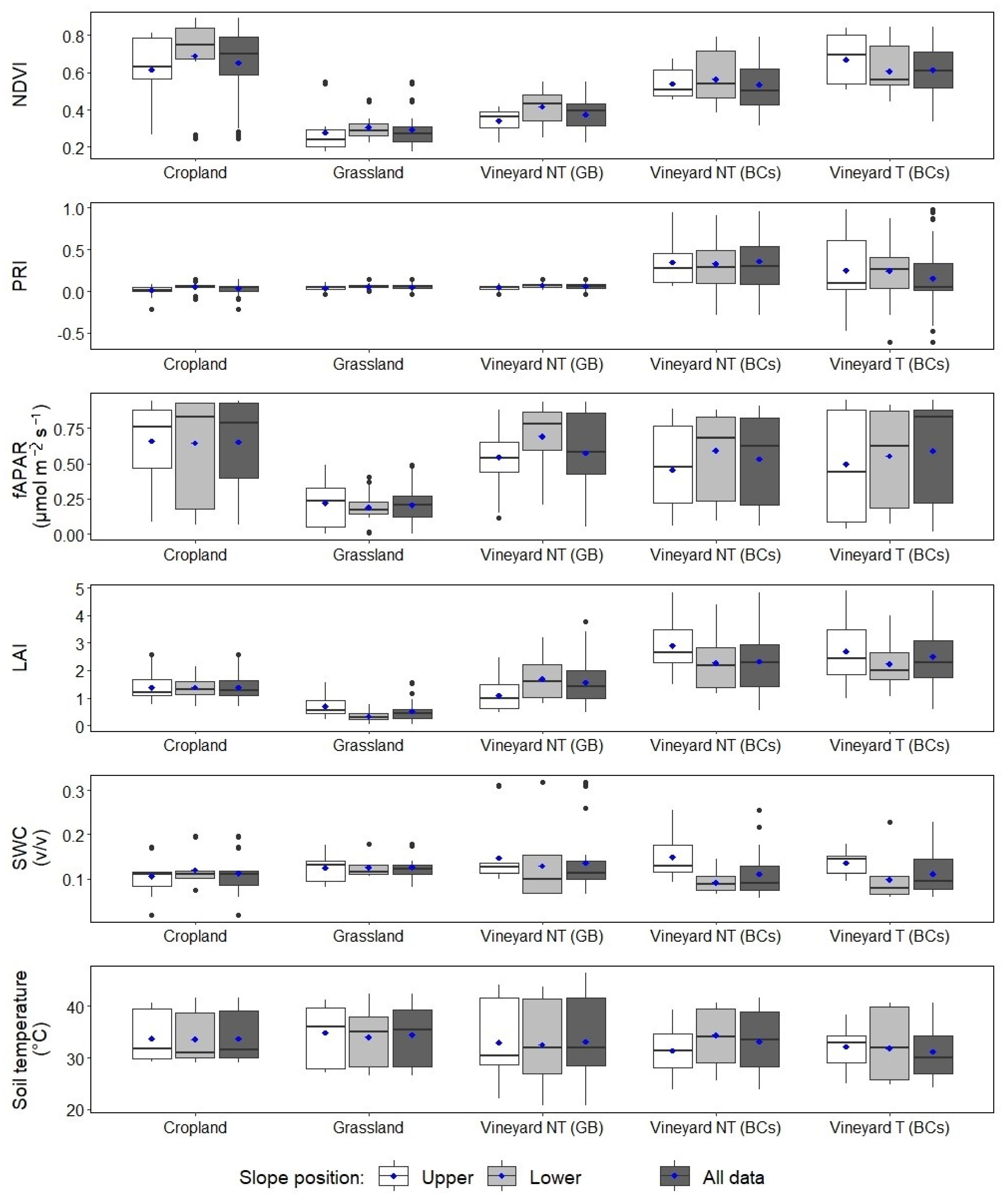
Our data show that slope position has a strong influence on plant parameters. The NDVI values were higher for plants at the bottom of the slopes for most land use types, except the tilled BCs vineyard. The highest overall NDVI was observed for the lower point of the cropland (0.690) and the lowest for the grassland upper point (0.280). The PRI values were similar for the BCs sites both at the bottom and upper points of the slopes (
Figure 4). The largest difference of the PRI values between the slope positions was observed for the maize (cropland), where plants at the lower part had over three times higher values compared to the upper point’s values. For the GB vineyard, the grassland and the cropland each had significantly different NDVI and PRI values between the slope positions. The fAPAR values between the slope positions showed clear differences, whereby the vineyard and cropland sites had higher values at the bottom than at the top (
Figure 4). However, these differences were not significant.
Based on the mean of the seven measuring dates, the soil water content was the lowest at the BCs no-till site lower point (9.15%), followed by the cropland upper point (10.55%). Remarkably, the highest average SWC was observed for the BCs no-till upper point followed, by the BCs tilled site’s upper point. The soil temperatures were similar between the upper and lower study points for most of the respective land use types. The soil temperature did not differ much, it was between 31.33 and 34.86 °C (BCs no-till upper point and grassland’s upper point, respectively).
The lowest average NDVI was measured for the grassland (0.293) and the highest for the maize (0.653); however, compared to the maize, the BCs sites had similarly high values observed. All NDVI values were significantly different among land use types (p < 0.001). The PRI values were much higher for the BCs sites compared to all other sites. Except for the BCs tilled and no-tilled sites, and between the GB and grassland, all land use types had significantly different PRI values (p < 0.05). The fAPAR values of maize and grapevine were similar (average for maize 0.645, and for the grapevines 0.548), while for grassland it was substantially lower (average 0.197). The highest average fAPAR value was observed for maize (0.645). Statistically, the grassland had significantly lower fAPAR values compared to the other land use types (p < 0.01), while most other sites were similar. LAI values were relatively low in all measured points due to the extremely dry and hot conditions in the study period. The highest overall values were observed for the two BCs vineyard sites (2.35 and 2.54 for BCs NT and T, respectively). The lowest LAI value was noted in the grassland (0.51). Interestingly, the slope upper points had higher LAI values compared to the lower ones, with significant differences (p < 0.01 for vineyards BCs NT and GB, and grassland), except for the cropland, where the overall values were very similar (p > 0.05).
The SWCs of the investigated land use types were relatively alike and varied between 11.2% and 13.7% for the measurement times. Statistically, only the grassland and BCs no-tilled site (p < 0.05) and grassland and cropland were significantly different (p < 0.01). Similar to the SWCs, the overall soil temperatures showed small variations, between 32.0 (BCs tilled) and 34.4 °C (grassland) during our measuring times, and the only significant difference was observed between grassland and BCs tilled sites (p < 0.01).
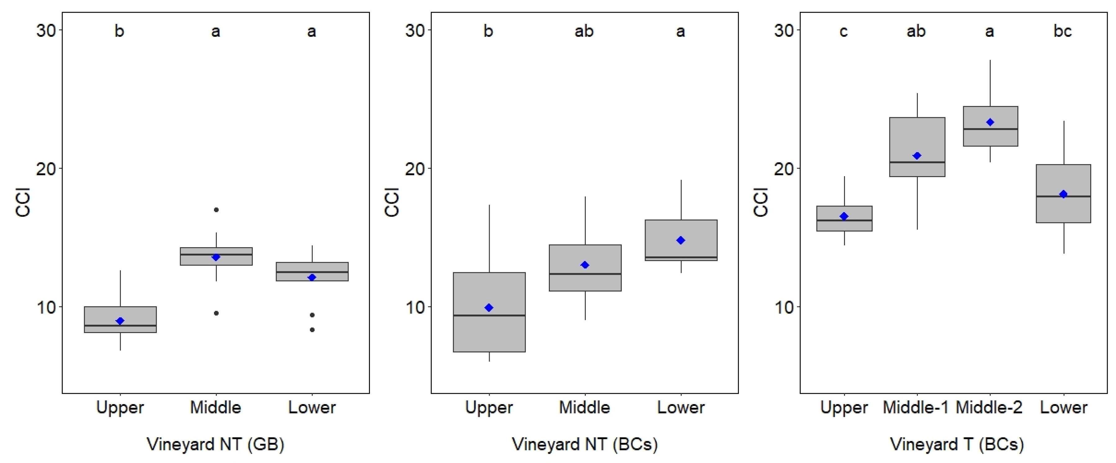
Leaf chlorophyll contents were measured for all three vineyard sites, and the content values are shown in
Figure 5. The highest chlorophyll contents were measured in the BCs vineyards’ tilled sites, while the lowest was observed for the GB vineyard. We found that slope positions significantly influenced the chlorophyll contents as the lower points’ values were significantly higher compared to the middle or the upper points’ data for the investigated slopes (
Figure 5).
3.2. Soil–Plant–Water Relations
To better understand the relationships between overall plant traits and soil characteristics, selected soil physical and chemical parameters were measured in the laboratory. The basic soil physical and chemical characteristics of the investigated land use types are summarized in
Table 1.
Among the land use types, cropland had the lowest sand concentration and one of the highest clay contents (
Table 1). The highest sand and lowest clay contents were observed for the BCs vineyards, showing that even though different soil management is being performed, the soil structure is still similar in the adjacent slopes. Soil pH was slightly basic for all land use types. Grassland had approximately three times higher nitrogen content compared to the other land use sites, along with the highest SOC content (
Table 1). Among the land use sites, cropland had the highest P
2O
5 and vineyard GB the highest K
2O content.
Correlation analysis was performed to see how strong the connections are between the investigated soil and plant parameters. Correlation analysis was conducted based on data from each land use type, separately.
NDVI and fAPAR values were well-correlated for the cropland (
r = 0.64;
p = 0.02), while NDVI and PRI showed a weaker, positive correlation in the vineyards (
r = 0.42;
p = 0.22;
Table 2). The LAI was well-correlated with the NDVI values for the cropland and the vineyards (
r = 0.51 and 0.83, respectively). The SWC was moderately correlated with the NDVI values for the vineyards (
r = 0.56;
p = 0.09) and showed no significant correlation with the selected parameters (
Table 2). Soil temperature negatively affected most of the plant parameters, especially SWC (
r = −0.25–−0.30;
Table 2).
Besides soil water and plant data, we included soil chemical measurements such as pH, soil organic carbon (SOC), total nitrogen, NH
4+, NO
3−, K
2O, P
2O
5, and C/N, as described in
Table 1. The results of the Pearson correlation analysis for plant parameters, soil water content, and soil temperature compared to soil physical and chemical values are summarized in
Table 3. For the vineyards, strong negative correlations were observed between NDVI and clay, SOC, N, K
2O, and NH
4−-N contents of the soil (
r > −0.63;
p < 0.01;
Table 3,
Figure 6). For the vineyard samples, NDVI had a strong positive correlation with soil pH (
r > 0.87;
p < 0.01
Table 3) and moderate correlations with sand, silt, and NO
3− contents (
r > 0.53). fAPAR values showed a moderate positive correlation with soil C/N for the cropland (
r = 0.52) and with P
2O
5 for the vineyards (
r = 0.58). From the soil physical parameters, sand had a positive effect (
r = 0.64;
p = 0.02), while clay had a negative influence (
r = −0.58;
p = 0.04) on the grassland’s PRI values.
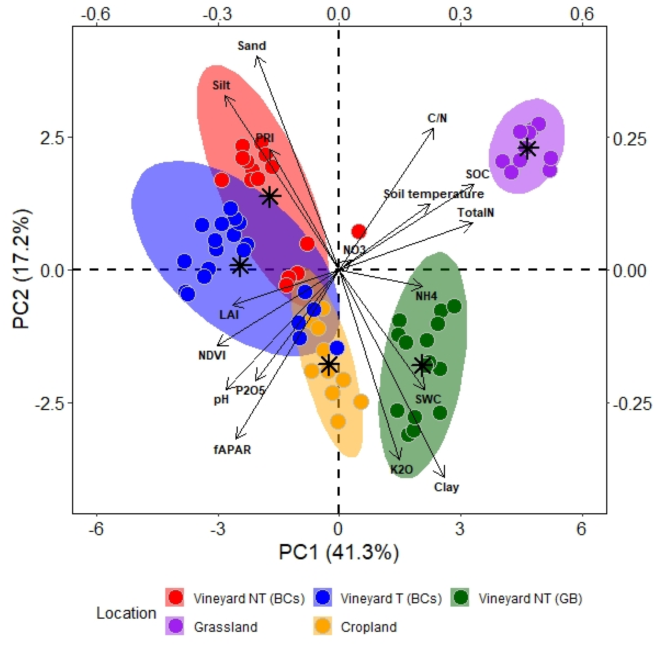
The PCA revealed that the first principal component (PC1) accounted for 41.3% of the variation caused by the interaction, while PC2 accounted for 17.2% (
Figure 6). The data show clear partitioning of grassland and vineyard GB samples from the vineyard BCs sites and cropland along the PC1, concurrent with partitioning of grassland from vineyard GB and cropland along PC2.
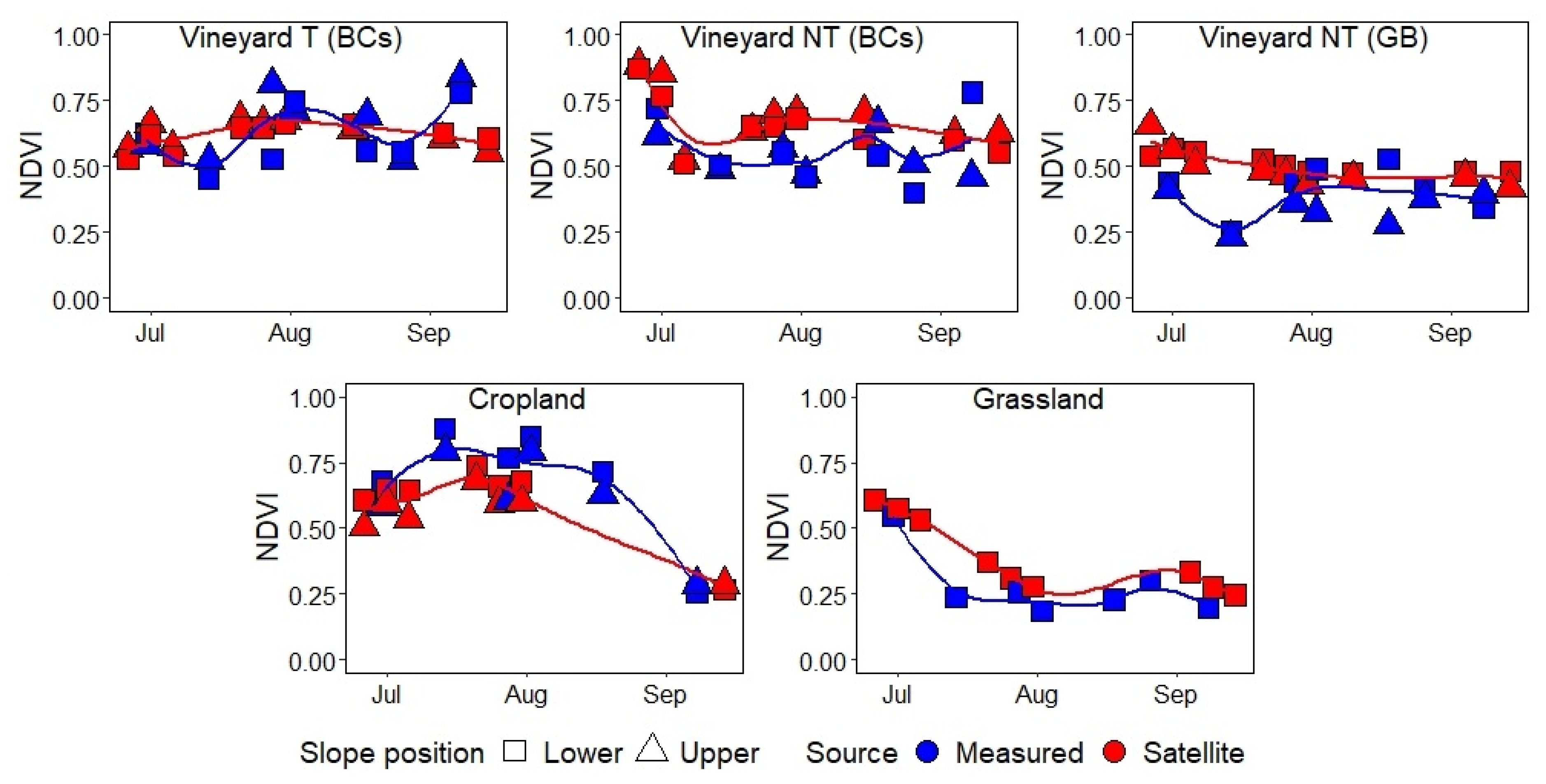
3.3. Remote Sensing Versus Field NDVI Measurements
Ground measurements and Sentinel-2 imagery were used to study NDVI values at each land use type and location. We found that for the GB vineyard and the grassland, our measurements were lower than the satellite-retrieved NDVI data (
Figure 7). For the cropland, our measurements had systematically higher estimated NDVI values compared to the Sentinel-2 values.
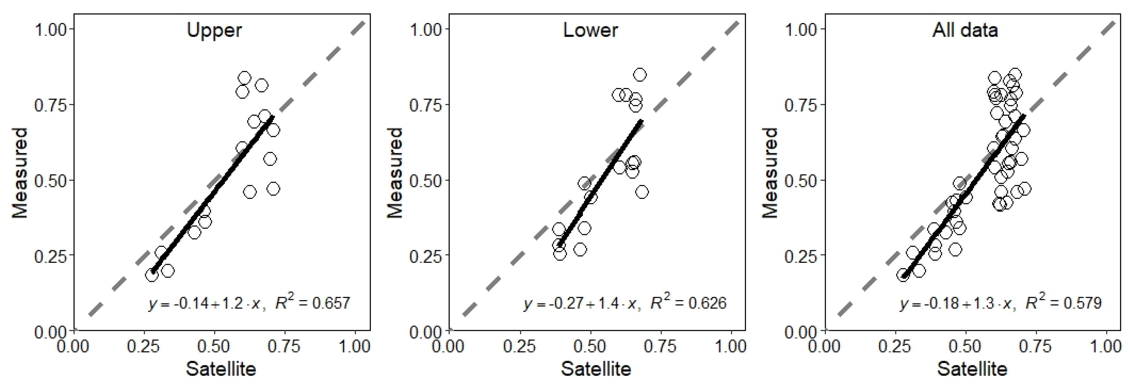
Figure 8 shows the correlation between the measured and satellite-retrieved NDVI values, where the different slope positions and the overall comparison are separately shown. The upper and lower measurement points showed very strong and strong correlations (
r = 0.811 and 0.791, respectively) when analyzed separately. Based on all the retrieved points, we found a strong correlation (
r = 0.761,
p < 0.001) between the satellite imagery-based and field-measured NDVI values (
Figure 8).
While most of the vegetation period was under dry conditions, a larger precipitation event (16.4 mm) occurred on 1 August, which increased the top 12 cm of the soil column from 9.4% to 21.5% average SWC for the study sites by 2 August, which was one of the field measurement days. We observed no significant differences between the NDVI values measured before and after the precipitation nor the satellite-retrieved NDVI data (p > 0.05).
4. Discussion
Monitoring plant responses to the changing environmental conditions might provide immediate knowledge on stress-related changes. Besides meteorological conditions, these changes can arise from soil nutrient or soil water content (SWC) deficiencies. The year 2021 was an exceptionally dry year for the study site, with 399.4 mm of precipitation in total measured at the study catchment outlet. During the investigated period (June–September), only three rain events had more than 10 mm of precipitation, which is below the average expected in this area [
38].
The physical properties of the soil can greatly influence SWC, as hydrological properties such as hydraulic conductivity are highly dependent on particle and aggregate size distribution. While the soil particle size distribution can vary with depth and position in a given land use type, the soil hydraulic properties can correlate well with soil pedological properties [
39]. Our study showed that at BCs sites, the slope position affected SWC, and at the lower points, SWCs were lower compared to the upper points. One of the possible reasons is that the upper points at this study site had 64% and 42% higher clay contents (T and NT, respectively) compared to the lower points, where finer grain sizes such as clay can hold more water during drought conditions [
40]. Dlapa et al. [
41] investigated pore size distribution and water retention differences of various land use types and found that grassland has higher water retention than arable land, concurrent with SOC content. Our study also highlighted that grassland and vineyard GB were the two land use types with the highest SOC contents, and they also had the highest SWC in the upper 12 cm of the soil layer. However, our SWC measurements were very similar between most of the measuring times, and therefore our deduction is not sufficiently supported without additional measures after larger precipitation events.
The PRI can be used to assess changes in leaf reflectance that can be an outcome of either soil nutrient- or water-related stress [
5,
9]. Higher PRI might be expected at low light intensity conditions as most light is being utilized by the plants, while the PRI might decrease at high light intensities [
42]. Our results indicate that increases in the SWC increased the PRI values, and therefore the studied plants suggest better light use efficiency at better soil water conditions. The overall PRI among land use types suggests that the cropland, grassland, and vineyard GB sites were under stress, while the grapes at the BCs vineyard sites showed the least distress. One of the most likely reasons for the differences is the root length. Grass and maize have the densest root structure in the upper 20–40 cm soil layer [
43], while grape roots can go as deep as 10–15 m [
44]. Therefore, during drought conditions when the top soil layer is very dry, the deeper grape roots can remove some soil water and nutrients. We also noted differences between the PRI values of the two vineyard sites. The GB vineyard has highly eroded topsoil, and therefore the grape roots are limited by the proximity of the bedrock, while the grape roots are not restricted in growth at the BCs vineyard site. Based on soil chemistry, we found no connections to the PRI variations. While we found weak connections between PRI and LAI values, others found strong relations [
45]; however, our data are limited to one vegetation period when mainly drought conditions were present.
The effects of temperature and precipitation changes on plant biomass production can be monitored using NDVI values. In our study sites, grassland was the driest, and the plants had not recovered after an early July mowing event, as was shown in the very low NDVI values both in the field measurements and satellite-retrieved data. The day after a larger precipitation event in August, we conducted a field measurement, however the NDVI values showed no significant differences compared to earlier values. Plant responses to the increasing SWC might take longer than a day to show differences in their physiology [
8], which also depends on the time water takes to infiltrate into the deeper soil layers where roots can uptake it. Drought conditions can result in decreasing NDVI values, as was observed in many studies [
4,
46,
47]. We found a strong correlation between fAPAR and NDVI values for the vineyards. A healthier canopy is not only greener but can also be denser, and therefore the connection between our parameters could be expected. NDVI is known to reflect in canopy changes, such as leaf movement or wilting [
48], and therefore it is a useful tool to detect overall plant structural changes. However, PRI is more suitable for plant physiological changes because it is better linked to the process of photosynthesis [
49]. The LAI and fAPAR values can correlate well, and both provide similar information on plant canopy and health. However, while fAPAR values were measured from the below-canopy and above-canopy values only, the LAI values were averaged from the top to bottom measurements for the grapevines and maize, and therefore weak positive correlations are acceptable.
The chlorophyll contents were measured for the three vineyard sites at a veraison stage. We found that slope position greatly affected the leaf chlorophyll content; however, soil management also showed high variations among the grape leaves’ chlorophyll values. Chlorophyll content can decrease under drought conditions; however, depending on the type of grapes, it might not be significantly affected [
50]. Tillage can also negatively affect the leaves’ chlorophyll content [
50]; conversely, in our study, we observed positive effects in the veraison stage. However, as leaf chlorophyll contents of grapes have high spatio-temporal variability [
51], more measurements should be performed at other phenology phases to better understand plant development. Chlorophyll contents can be strongly correlated to NDVI and PRI values [
45], and therefore further measurements would enable us to establish more profound deductions. Soil chemistry influences plant growth, and the addition of nutrients to the soil can help in plant development. In many vineyards, organic or inorganic fertilizer or compost addition might be applicable. High carbon and NPK concentrations in compost can increase soil quality for plants, and consequently, increase the chlorophyll concentrations of the grapevine leaves [
52].
During summer months, SWC and air temperature are the main factors affecting NDVI [
53]. High soil temperature increases evaporation rates, which consequently reduces water infiltration into the deeper layers of the soil. SWC did not correlate well with our plant parameters of NDVI, PRI, or fAPAR, except for the vineyards. The magnitude of the correlations between NDVI and SWC or soil temperature values highly depended on the vegetation type. Cui et al. [
54] found positive and significant correlations between NDVI and temperature and weak negative, non-significant correlations between NDVI and precipitation. In our study, we only investigated soil temperature and water content, however, with NDVI and soil temperature, we found mixed results of both negative and positive weak correlations depending on vegetation types. In the present study, the SWC and temperature values were based on the top 12 cm of the soil column and were highly dependent on the time of the measurements. During the study period, there was a long drought period along with high air temperatures. These factors limited our ability to fully investigate the effects of SWC and soil temperature on the plant parameters under study. Therefore, more frequent measurements, especially before and after rain events or longer cold front events, might provide more precise deductions.
Satellite- and field-based NDVI measurements showed a strong correlation in our study. However, the Sentinel-2 satellite-based imagery used 100 m
2 data, compared to our handheld sensors with a maximum of 2.07 m
2 per measurement point depending on the plant type and height. While for the grassland and maize after canopy closure, both methods can approximate good correlations, for the vineyard sites, the row spacing includes either grass or cover crops. To overcome alterations in the integrated NDVI values, corrections to the solar elevation (e.g., the sunlit and shaded soil) should also be considered [
55]. Therefore, for the vineyards and croplands prior to full canopy development, the handheld instrument can be a great tool to assess the differences between overall site-specific values. On the other hand, the handheld sensor set only measures certain spectra of the reflected lights, while the satellite imagery enables us to capture more vegetation indices, such as the enhanced vegetation index (EVI), soil-adjusted vegetation index (SAVI), or the chlorophyll vegetation index (CVI). These additionally derived indices can be used to further enhance our knowledge on site-specific plant growth and development.
5. Conclusions
The soil–plant–water system was investigated by establishing soil physical, chemical, and hydrological characteristics along with plant traits of NDVI, PRI, fAPAR, LAI, and leaf chlorophyll content. In our study, the highest stress conditions for plants were observed for the grassland site, where most plant parameters were much lower compared to the vineyard or cropland sites (e.g., NDVI, fAPAR, LAI). We found that slope position can significantly influence plant development due to soil management or erosion-related soil physical and chemical changes. Therefore, our results highlight the importance of soil–plant–water relationships and their interactions, as soil property changes due to environmental conditions result in changing parameters for plants to grow, or by the plant itself by taking up nutrients from soil or developing dense root structures. Slope position also showed clearly distinguishable results on grapevine leaf chlorophyll concentrations, as the plants located at the slope upper positions had significantly lower chlorophyll levels compared to the plants at the lower points. The soil temperatures were generally higher at the upper points of a given slope, which increases evaporation and can consequently decrease SWC at lower soil layers. Therefore, careful evaluation should be conducted in these areas prior to crop sowing. In addition to ground measurements, we also analyzed satellite imagery and noted a strong correlation between the collected values. We found that incorporating satellite imagery into our analysis could greatly improve and add depth to our findings. Nevertheless, this study is the first analysis on the area of concern, and the in situ measurement methods and the use of satellite imagery can be further refined. Our field measurements were carried out in an exceptionally dry year, when SWCs were very low and soil and air temperatures were high. To draw more accurate conclusions, additional measurement points from a wetter growing season or even after wetter weather periods should be included. We also plan to extend the study with multiple vegetation indices on a spatio-temporal scale.


