Long-Term Assessment of Spatio-Temporal Landuse/Landcover Changes (LUCCs) of Ošljak Island (Croatia) Using Multi-Temporal Data—Invasion of Aleppo Pine

Abstract

The karst landscapes of the Mediterranean are regarded as some of the most vulnerable, fragile, and complex systems in the world. They hold a particularly interesting group of small islands with a distinctive, recognizable landscape. The Republic of Croatia (HR), which has one of the most indented coasts in the world, is particularly known for them. In this paper, we analyzed the spatio-temporal changes (STCs) in the landscape of Ošljak Island, the smallest inhabited island in HR. Landuse/landcover change (LUCC) analysis has been conducted from 1944 to 2021. The methodology included the acquisition of multi-temporal data, data harmonization, production of landuse/landcover (LU/LC) maps, selection of optimal environmental indicators (EIs), and simulation modeling. In total, eleven comparable LU/LC models have been produced, with moderate accuracy. STCs have been quantified using the nine EIs. The dominant processes that influenced the changes in the Ošljak landscape have been identified. The results have shown that, in recent decades, Ošljak has undergone a landscape transformation which was manifested through (a) pronounced expansion of Aleppo pine; (b) deagrarianization, which led to secondary succession; and (c) urban sprawl, which led to the transformation of the functional landscape. The most significant of the detected changes is the afforestation of the Aleppo pine. Namely, in a 77-year span, the Aleppo pine has expanded intensively to an area of 11.736 ha, created a simulation model for 2025, and pointed to the possibility of the continued expansion of Aleppo pine. Specific guidelines for the management of this new transformed landscape have been proposed. This research provides a user-friendly methodological framework that can efficiently monitor LUCCs of a smaller area in the case when geospatial data are scarce and satellite imagery of coarser resolution cannot be used. Moreover, it gives an insight into the availability and quality of multi-temporal data for the HR.

1. Introduction and Background

The analysis of landuse/landcover changes (LUCCs) [1] is very important to understanding the relationship between the socio-economic development of specific areas and the balance of the landscape [2]. This type of analysis is conducted with the aim of identifying changes in thematic attribute [3] at a specific study (time) period, within a specific (area) landscape. The thematic attribute can refer to (1) land cover (LC)—which concerns the properties of features (objects, patches) at the surface, and (2) land use (LU)—which describes the socio-economic function of that features (patches) at the surface [3]. LUCCs analysis helps to establish a deep insight into the past appearance of the. LUCCs primarily allude to the effects of human activity on a specific ecosystem or landscape [4]. Furthermore, the significant LUCCs in larger areas can have a direct impact on biodiversity, biogeochemical cycles, sustainable use of environmental resources, and interactions between biosphere-atmosphere [5]. Vegetation can have a significant effect on hydrological fluxes due to variations in the physical characteristics of the land surface, soil, and vegetation, such as the roughness, albedo, infiltration capacity, root depth, architectural resistance, leaf area index (LAI), and stomatal conductance [6,7].

LUCCs have been the object of research by numerous scientists in recent decades. It is necessary to analyze LUCCs in order to determine temporal trajectories of LU/LC change [8]. This can generate information about landscape dynamics that can be crucial to understanding human–environment interactions. In order to do that, the fundamental step is to acquire the multi-temporal spatial data over an observed research area [9]. Therefore, LUCC analysis has been performed for the landscapes in almost all continents around the world, using the different sources of spatial data, within various time periods, by applying different methodological complexity. For example, ref. [10] used various geospatial technologies to monitor LUCCs in a Mediterranean wetland of northern Greece, ref. [11] analyzed the historical and future spatial patterns of classes in the Central Alps, and ref. [2] analyzed LUCCs in South Tyrol (Italy). There are numerous studies of the LUCCs for Northern, Central, and South America. For example, ref. [12] analyzed LUCCs for the city of Mississauga on the shore of Lake Ontario (Canada), ref. [13] analyzed the urban landscape of the Phoenix metropolitan region, and ref. [14] analyzed LUCCs for the northeastern coast of Florida. Furthermore, ref. [15] accelerated the process of harmonizing the satellite imagery in order to perform the LUCCs analyzes using forest cover in Minnesota; ref. [16] analyzed, quantified, and compared spatial urbanization processes for the four largest Mexican urban agglomerations; and ref. [17] assessed spatio-temporal rates and patterns of LU/LC changes in the Cerrados of southeastern Mato Grosso, Brazil.

Multi-temporal geospatial data in LUCCs analyses include data collected using various methods and sources, such as historical cadastral maps, satellite imagery, historical aerial photographs (HAPs) [18,19,20], field surveys, and unmanned aerial vehicle (UAV) photogrammetry. If the LUCCs are observed further back in time, various old maps such as cadastral maps can be consulted. However, such maps are less reliable considering the technical capabilities of that time and need to be harmonized with newer data. HAPs are regarded as the oldest form (the early 1930s) of remote sensing data [21] and are recognized as valuable historical information and a unique resource on vegetation dynamics [18] that can provide essential referent data for quantitative mapping of landscape heterogeneity within a specific time period [22]. However, it is necessary to point out technical constraints of this source in LUCC analysis, including the lack of ground control data necessary to assess the accuracy of the model, as well as precise camera parameters, which could hamper an orthorectification of the raw imagery. Therefore, the historical aerial grey-scale photographs (HAPs) and orthomosaics collected by official state geodetic administrations using high-resolution cameras mounted on aircraft [10,12,14] and, in recent times, by UAV [23] provided constant and detailed insight into LUCCs. Since the mid-1970s, the increasing availability of long and short time series satellites (e.g., Landsat and Sentinel series) and available archival satellite data have simplified the performance of LUCC analysis, systematic monitoring of landscape changes [9,14,24], and advanced land change science [8]. However, the previously mentioned freely available satellite images cannot be used in the analysis of LUCCs for smaller areas due to their spatial resolution (medium 10–30 m). Therefore, if smaller areas are analyzed, other data sources need to be used. Today, a new incentive is coming with the development of UAVs and accompanying sensors (red, green, and blue—RGB; multispectral; and hyperspectral cameras) that can monitor LUCCs on bigger scales or at higher spatial resolutions. When a large amount of spatial data of different spatial resolution is available for a larger area, multiple-scale validation processes are encouraged. This allows the scientist to determine if the model LUCCs makes predictions at scales that are relevant to the purpose of the research [25].

Due to the various differences between the mentioned multi-temporal datasets, data harmonization must be performed [15,26]. These differences can include different spatial coverages, viewing and solar angles, and atmospheric conditions [27], as well as different spatial, spectral, and/or radiometric properties [15]. That being said, it is almost impossible to perform LUCC analysis without the use of multi-sensor data over extended periods of time. For example, ref. [14] used satellite and aerial photogrammetric data for analysis of mangrove–saltmarsh ecotone changes for the 1942–2013 period, and ref. [28] used topographic maps, satellite, and aerial photogrammetric data for LUCCs analyses for Nepal between 1978 and 2010.

Modern geospatial technologies (GSTs) have made it possible to accurately detect and track changes in the landscape [29,30,31,32,33]. As a result, a wide spectrum of environmental indicators emerged which are intended for the precise quantification of the current state of the landscape or any part thereof [33,34,35,36]. Environmental indicators are used to identify the state of the landscape, early-warnings of ecological problems, and the state of ecological resources [37]. They are measures of the size, shape, and spatial proximity of specific land types, as well as the configuration and complexity of all land types within an area [38]. Various landscape indicators have been discussed in many papers [39,40,41]. The United States Environmental Protection Agency (EPA) has singled out and explained several indicators for the recovery potential screening (RPS) ecological indicators category [36]. The choice of environmental indicators to be used in LUCC analysis depends on the characteristics of the available multi-temporal data and derived models.

Nowadays, simulation modeling of LUCC is becoming very popular. Simulation modeling is a method used to explain and project LUCCs that are basically related to broader social and natural elements [42]. They are one of the most effective tools for studying LUCCs and can further support LU planning and policy [43]. Numerous researchers around the world are working on the development of LU/LC simulation models [44,45,46,47,48,49,50,51]. Most empirical research based on LUCC simulation models has focused on dynamic areas that have experienced significant changes, such as rapid population growth, urbanization, and economic development in recent decades [52]. However, there are almost no similar researches in the territory of the HR. Only [42] conducted simulation modeling of LUCCs for Požega-Slavonia County (HR) for the period from 1985 to 2027.

The Mediterranean region is considered as one of the most endangered ecosystems in the world, whose landscape is undergoing major changes [53,54]. It is under the constant influence of various natural endogenous and exogenous processes, and, as such, is subject to constant change [55,56]. Landscape changes are occurring with increasing frequency due to the different driving forces, such as socio-economic, cultural, political, and technological factors [57]. Therefore, increasing pressure on natural resources [2,58] require sustainable solutions to preserve this and other fragile ecosystems. Within the Mediterranean region, the karst landscapes are especially regarded as some of the most vulnerable, fragile, and complex systems in the world [59,60].

The HR is particularly recognized for its karst landscapes. Most of them are, according to the International Union for Conservation of Nature (IUCN) classification, protected areas according to their management objectives, and even some are included in the United Nations Educational, Scientific, and Cultural Organization (UNESCO) World Heritage List. The HR has one of the most indented coasts in the world and more than 1248 islands, islets, and reefs [61]. Croatian islands are a great economic resource for the Croatian economy; as such, they should be monitored and preserved through smart and sustainable management. Considering its geographical location and predominant climatic type, Croatia should be completely overgrown with forest [62]. However, as in the rest of the Mediterranean, human activity has created a specific landscape characterized by the almost total disappearance of indigenous vegetation of holm oak and the predominance of other degrading or invasive forest species [63].

The LUCCs in HR were mainly influenced by the actions and policies caused by socio-economic situations. Depopulation, mainly caused by emigration from island rural areas toward nearby urban coastal cities and other immigration destinations in HR and in highly developed countries, followed by the collapse of socialism and the Homeland War in the early 1990s, led to major socio-economic and institutional changes [64]. The orientation of the Croatian economy exclusively towards tourism has also led to an uncontrolled litoralization of the Croatian coast and islands, accompanied by mass, and sometimes illegal, apartmentization and betonization [65,66]. All this led to de-agrarianization and afforestation of rural areas of the HR [67]. Accordingly, most of the Croatian islands have experienced such a fate. Many arable lands have been abandoned and left to the spread of the indigenous Mediterranean and non-indigenous vegetation, especially Aleppo pine [68]. Considering the prevailing socio-economic processes, small inhabited islands stand out the most. During historical and geographical development, they developed a specific “metabolism” ([69], p. 32), thus relying on local and individually modest resources which form specific landscapes [70]. Therefore, special emphasis in LUCC analysis can be placed on small Croatian islands, i.e., fragile socio-economic communities that have developed on the periphery in relation to the centers of decision-making. In recent decades, they have undergone a radical transformation which was manifested through depopulation in the island demography, economic disorientation, and LUCCs which influenced the change in the island functions [70]. However, before this, the landscape of the Croatian islands was recognizable by cultivated olive groves and vineyards, carefully landscaped gardens, and maintained roads that made every part of the island accessible. Numerous historical sources testify to this, especially A. Fortis in 1774 and L. F. Cassas and J. Lavalle in 1802 [71].

One of these landscapes was Ošljak, the smallest inhabited island in HR. Therefore, the main objective of this paper was to analyze the LUCCs of Ošljak Island over a 77-year period (1944–2021). Moreover, an analysis of changes in the number and distribution of cadastral parcels was made for the 246-year period (1776 to 2022). The main challenge in this research was the fact that free satellite images (e.g., Sentinel and Landsat) could not be used as input data for LUCC analysis due to the size of the study area (33.5 ha) and the study period. Therefore, it was necessary to acquire the other available multi-temporal data, which included cadastral maps, historical aerial photographs (HAPs), and UAV imagery. This demanded a large amount of time and resources. Furthermore, the characteristics (spatial, spectral, and radiometric resolution) of these data required the conduction of the data harmonization process and conditioned the number of classes of the LU/LC models and the type of selected environmental indicators used to monitor the state of the Ošljak landscape. In the context of studying the landscape functional transformation, which can be regarded as a research gap, it is necessary to point out that attempts to analyze landscape functions transformation based on LC information can be limited since the LC is not always a good indicator for the actual functions performed by the land [43,72].

In summary, in the analysis of STCs of the Ošljak landscape, multi-temporal data from 1776 to 2021 were acquired from different sources. The paper seeks to present a user-friendly methodological framework that can efficiently monitor LUCCs of a smaller area in the case when geo-spatial data are scarce. The secondary objectives of the research were:

(a)

to collect and harmonize different acquired raster data;

(b)

to perform comparable LU/LC models for the defined time period;

(c)

to derive the latest (2021) LU/LC model of the Ošljak Island;

(d)

to define appropriate environmental indicators (EI) in LUCC analysis;

(e)

to determine the dominants changes in LU/LC within a defined period

(f)

to identify the reason that caused these changes;

(g)

to create a stochastic simulation model from 2018 to 2025;

(h)

to provide basic guidelines for the management of Ošljak.

Furthermore, this research provides insight into the availability and quality of some multi-temporal data for the territory of the HR, as well as how to harmonize it and perform LUCC analysis in order.

Study Area

The island of Ošljak (Figure 1C) is the smallest Croatian-inhabited island (

Table 1. The number of Ošljak inhabitants in the period 1857–2021.

Island	1857.	1869.	1880.	1890.	1900.	1910.	1921.	1931.	1948.	1953.	1961.	1971.	1981.	1991.	2011.	2021.
Ošljak	45	50	62	87	91	85	130	199	139	125	93	64.	27	65	18	37

Source: [74].

) with an area of about 0.33 km² [73] located in Zadar County, more precisely in the Zadar channel (Figure 1A). According to the administrative territorial structure of HR, it is classified as a settlement [74] which belongs to the Municipality of Preko. Geographically, Ošljak belongs to the North Dalmatian island group, a subgroup Zadar archipelago [75] (Figure 1B). It is located about 780 m from settlement Kali, about 940 m from settlement Preko on the Island of Ugljan, and 4.5 km from the city of Zadar (Figure 1).

The length of the Ošljak coastline determined by UAV photogrammetry performed within this research is 4.18 km, while the highest peak is 88.5 m high (Štandarac). The coastline is more than twice as long as the line corresponding to the circumference of the circle (2052.9 m) whose area is equal to the area of the island. Due to the fact that there is no deeper bay on the island that would be sheltered from the winds, the residents built a seawall on the west coast of the island and arranged part of the coast for mooring ships which includes a smaller boat ramp for pulling boats out for maintenance and repair. Furthermore, the oldest monuments of profane and sacral architecture are concentrated next to the port. The ferry port, a key element of modern port infrastructure in Ošljak, has also been arranged at this location.

The first mention of the name Ošljak (Osglach) dates back to 1414 [76]. Ošljak owes its second name, Lazaret, to the fact that there was once a quarantine (built in 1630) where patients infected with the plague were brought to be cured or to die [77]. In addition to these two names, other names of the islet, such as S. Marco and Calogerà/Calugerà, have been recorded in archives and old maps during the 18th and 19th centuries [78], after the family that owned the island in the first half of the 18th century.

In the karst relief structure, the parallelism in the Dinaric direction (NW-SE) of the forms is expressed which indicates the Dalmatian type of coast. The island is dominated by carbonate rocks, while the pedological resources, flysch, and other softer sediments are exceptions. The dolomite agrarian-valued areas are mostly conveniently facing south. The main island development resource is the soil that developed on the predominant Cenomanian dolomites from which the nearby northeastern part of the island of Ugljan was built. These soils are mostly developed on slopes of smaller slopes in lower altitude classes. Half of the island’s surface is at altitudes of 0 to 20 m, and this zone borders the central island hill. The island of Ošljak is characterized by a Mediterranean climate with long, dry, and warm summers, and short, mild, and humid winters. The average annual temperature is about 14.7 °C. The average temperature in the coldest month of the year (January) is around 6.7 °C, while the average temperature in the warmest month (July) is 23.6 °C [79]. Although the total amount of precipitation is relatively high (915 mm), most precipitation (in the form of rain) falls in the colder months, mostly in November (118 mm), and the least precipitation falls in the warmest months, in July (35 mm). The vegetation cover of Ošljak belongs to the Mediterranean littoral belt. This area is commonly characterized by evergreen holm oak forests and Aleppo and black Dalmatian pine [80]. Therefore, the natural vegetation that predominates on Ošljak includes a mixed forest of Aleppo pine, cypress, and holm oak along with olive trees, Mediterranean macchia, and karst pastures. The cultivated vegetation is dominated by olive groves, vineyards, orchards, and vegetable gardens surrounded by dry stone walls. This significant landscape is home to several endangered and strictly protected bird species [81].

Ošljak is regarded as a place of great natural and cultural heritage; therefore, in 1985, it was included in the protected areas as a significant landscape [82] which corresponds to the fifth level (V.) of the IUCN protection category. This category (V) represents the landscape where, through time, human–nature interaction has produced a specific feature with significant biological, cultural, ecological, and scenic value [83]. In the significant landscape, interventions and activities that do not violate the characteristics for which it was declared are allowed. The Island of Ošljak is an example of traditional Mediterranean architecture with an old fishing port and the church of St. Mary dating from the 6th century. The hiking trail on the island is around two kilometers long, passing by a lighthouse and the remains of a windmill from the 17th century. This landscape is the basis for various forms of valuation—from the protection of biodiversity and cultural landscape to the management of these assets in the island’s development mechanism.

2. Materials and Methods

The methodology of this research can be divided into several steps (Figure 2). First, (1) multi-temporal data for STCs of the Ošljak landscape were collected using various methods and sources. These include (a) historical cadastral maps, (b) historical aerial photographs (HAPs), (c) field surveys, and (d) UAV photogrammetry. The total time period within which the multi-temporal data were collected was 245 years, ranging from 1776 to 2021. However, a detailed analysis of LUCCs for multiple classes (n = 6) was made for the period from 1944 to 2021 (77-year span) (Figure 3). This was conditioned by the characteristics, i.e., the detail of the available data. Urban sprawl and analysis of cadastral parcels were made for the period from 1776 to 2021 (244 years).

Since these data originate from different sources and were acquired using different inventory techniques, the process of (2) data harmonization was carried out in order to make comparable LU/LC models. Namely, each dataset has its own domain of applicability and quality standards [84].

In the (3) step, LU/LC models for the period of 1944–2021 were derived from the collected historical aerial photographs (HAPs) and digital orthophoto (DOP) of Ošljak (2021) in order to conduct LUCC analysis. The resolution of the LU/LC models was adjusted to the quality of the oldest HAPs; therefore, the ground sampling distance (GSD) of the model was 0.5 m. Within this step, an assessment of the thematic accuracy of each derived LU/LC model was performed using a confusion matrix and supporting metrics.

Then, in the fourth step, the appropriate (4) environmental indicators (EI) were selected in order to accurately detect and track changes in LU/LC models through the study period. The main condition for the selection of the appropriate EIs was to effectively indicate the state of the landscape and to point out the possible emerging problems. Furthermore, EIs were selected in regards to the characteristics of available multi-temporal data and quality of the derived LU/LC models.

In the final (5) step, LU/LC simulation models were performed using Modules for Land Use Change Simulations (MOLUSCE) plugin in QGIS. The objective of this was to generate the stochastic simulation model of the Ošljak landscape from 2011 to 2025. Special emphasis in this step was placed on monitoring, i.e., the simulation of possible further spread of Aleppo pine in the future (Figure 2).

2.1. Multi-Temporal Data Acquisition

In order to conduct the STCs analysis, it was necessary to acquire data from the 277-year period to gain the best insight into LUCCs. First, historical cadastral maps were collected whose level of detail was not good enough to perform STCs of landcover for multiple classes. The only usable LC class from this dataset was Urban (Figure 2). Therefore, multi-temporal HAPs were collected for detailed LUCC analysis (Figure 2). We have acquired a total of ten HAPs of Ošljak in the period from 1944 to 2018. These data can provide a great insight into the LUCCs over a period of 74 years, and when data from the 2021 UAV survey are added, the time period reaches 77 years.

2.1.1. Cadastral Maps

Cadastral maps can contain a lot of information about the area shown on them. By using them, it is possible to analyze part of this historical space; thus, they have a unique value in the reconstruction of historical, geographical, social, demographic, economic, and urban change over time [85]. Therefore, the acquisition of different cadastral maps, from 1776, 1824, and 2020, was carried out in order to reconstruct landscape changes in terms of urban sprawl monitoring and parceling, i.e., fragmentation of arable land on the island (Figure 2).

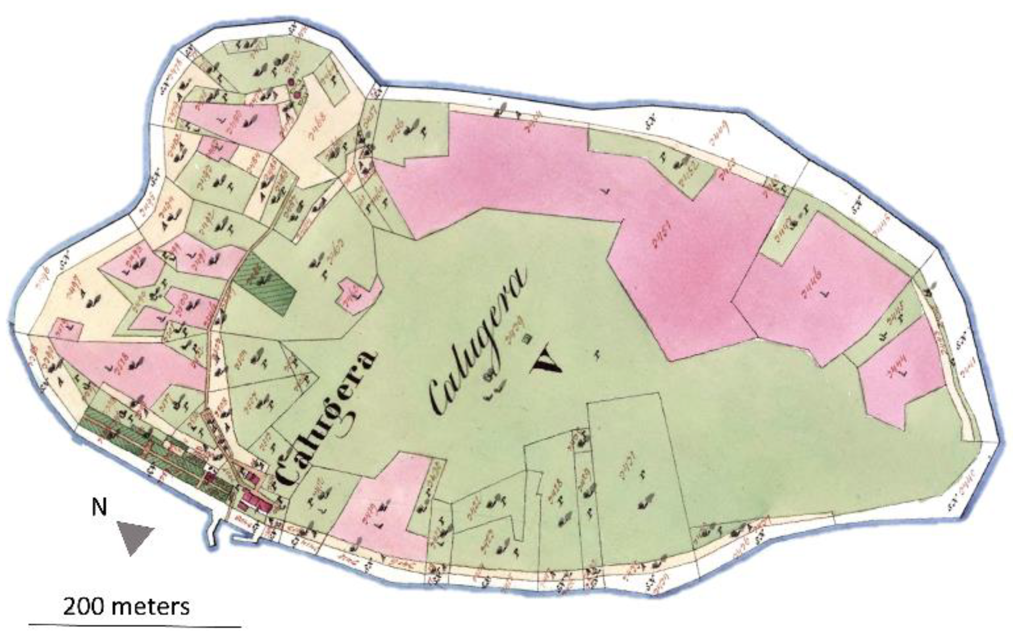
The map from 1776 is the oldest acquired data, representing the Plan of Ošljak (Pianta del Scoglio Osgliach) on 17 October 1776 (Figure 4). The copy of this map was made by the public surveyor and owner of the island Lorenzo Licini Rubčić [86]. Licini Rubčić was an excellent surveyor and cartographer, and it can be assumed that he carried out geodetic activities on his Ošljak with special care, as indicated by a very precise representation of the coastline. This plan is part of the Venetian cadastral created on the basis of orders issued by the general governors in the periods during the 17th and 18th centuries [85].

The second cadastral map dates from 1824 (Figure 5). More precisely, it is a sheet of the cadastral plan of the cadastral municipality of Preko made within the Franciscan cadastral survey of 1824 [87]. This map was made as part of the systematic cadastral survey of the countries of the Habsburg Monarchy, which for the first time included all Croatian lands. The survey was named as the Franciscan Survey after Emperor Francis I [78]. The cadastral from 2020 was acquired from the State Geodetic Administration (DGU). The DGU is the state geodetic administration of HR that performs administrative and other tasks related to geodetic and cadastral activities, in particular the preparation, renovation, and maintenance of the real estate cadastral; computerization of the cadastral and geodetic spatial system; topographic survey and state maps; management geodetic documentation; keeping statistical data of the real estate cadastral and infrastructure; etc.

2.1.2. Historical Aerial Photographs (HAPs)

Aerial imagery is acquired by periodic aerial surveys with a camera attached to a gyroscopically stabilized stand mounted above the opening in the bottom of the aircraft. Advances in GST have certainly revolutionized LUCC analysis; however, this technology has traditionally ignored greyscale (black and white) aerial photography [88]. Although the first aerial surveys of certain parts of Croatia began in the early 1930s, the first systematic aerial photogrammetric surveys were conducted after World War II [89]. The first available aerial photograph of the Ošljak Island used in this research was one acquired from a British Air Force dating from 1944 (World War II aerial photograph, photo no. 4103). It is preserved in the Croatian Hydrographic Institute (Figure 6). In this image, even before the LU/LC models were derived, dense drywall networks and the absence of high vegetation, i.e., forests, can be observed.

Furthermore, the HAPs acquired by the Military Geographical Institute (VGI) in Belgrade were collected for the years 1959, 1967, 1972, and 1977 (Figure 7). VGI has produced various types of cartographic, aerial, graphic, and textual–numerical documents in digital and printed form since 1876. Given that the HR was part of Yugoslavia, data from the period between World War II and the independence of the HR in 1991 are the legacy of the VGI. The newer LU/LC models ranging from 1997 to 2018 for the Ošljak were created based on archived aerial photos of the DGU. Aerial imagery for 1997, 2004, 2011, 2014, and 2018 were collected (Figure 7). The aerial photos are created as part of the systematic aerial survey of the entire territory of the HR, regularly carried out by the DGU every few years [90]. The request for obtaining aerial photogrammetric material is available at [91].

Over the years, the scale of aerial photogrammetric surveys and the type of metric cameras have changed depending on the availability and purpose of the surveys. Gradually, cameras with better technical specifications were developed, which allowed better resolution of the collected images and detection of smaller details on the images. Therefore, when using the available archive aerial imagery, the technical specifications of the cameras should be considered. An overview of used cameras is given in

Table 2. Overview of aerial photogrammetric data acquired for LUCC analysis of Ošljak island.

Data Type	Year	Camera Model	No. of Photos
Digitized analog aerial photograph	1944	N/A	1
Digitized analog aerial photograph	1959	SN Camera—RC8 343	1
Digitized analog aerial photograph	1967	N/A	1
Digitized analog aerial photograph	1972	N/A	1
Digitized analog aerial photograph	1977	N/A	1
Digitized analog aerial photograph	1997	Leica RC-20 15/4 UAGA-F	1
Digitized analog aerial photograph	2004	Carl Zeiss RMK Top 15	1
Digital aerial photograph	2011	Vexcel Imaging GmbH UltraCam X	1
Digital aerial photograph	2014	Vexcel Imaging GmbH UltraCam Condor M1 f80	1
Digital aerial photograph	2018	Vexcel Imaging GmbH UltraCam Eagle M3 f100	1

.

2.1.3. UAV Photogrammetry

The latest digital orthophoto (DOP) used for derivation of LU/LC model was generated based on UAV imagery collected in May 2021. The Matrice 210 RTK V2 and the 16 mm Zenmuse X7 camera were used in the UAV survey. The flight missions were planned in the DJI Pilot app. The percentage of front and side overlap was set at 80%. Considering the morphometric and vegetation characteristics of the island, the flight altitude of the UAV was set at 130 m above ground level (AGL), which resulted in the high resolution (GSD = 3.4 cm) of DOP and a digital surface model (DSM). The proposed flight speed was reduced to obtain better images, i.e., to avoid possible blurring at the edges of the missions at the moment when the UAV abruptly turns or stops. In addition, the camera settings (ISO, shutter speed, and aperture) were adjusted during the survey according to examples of good practice. Six ground control points (GCPs) were used for the orientation of the reconstructed model, and their coordinates were acquired using a high-precision Stonex S10 GNSS receiver (Figure 8).

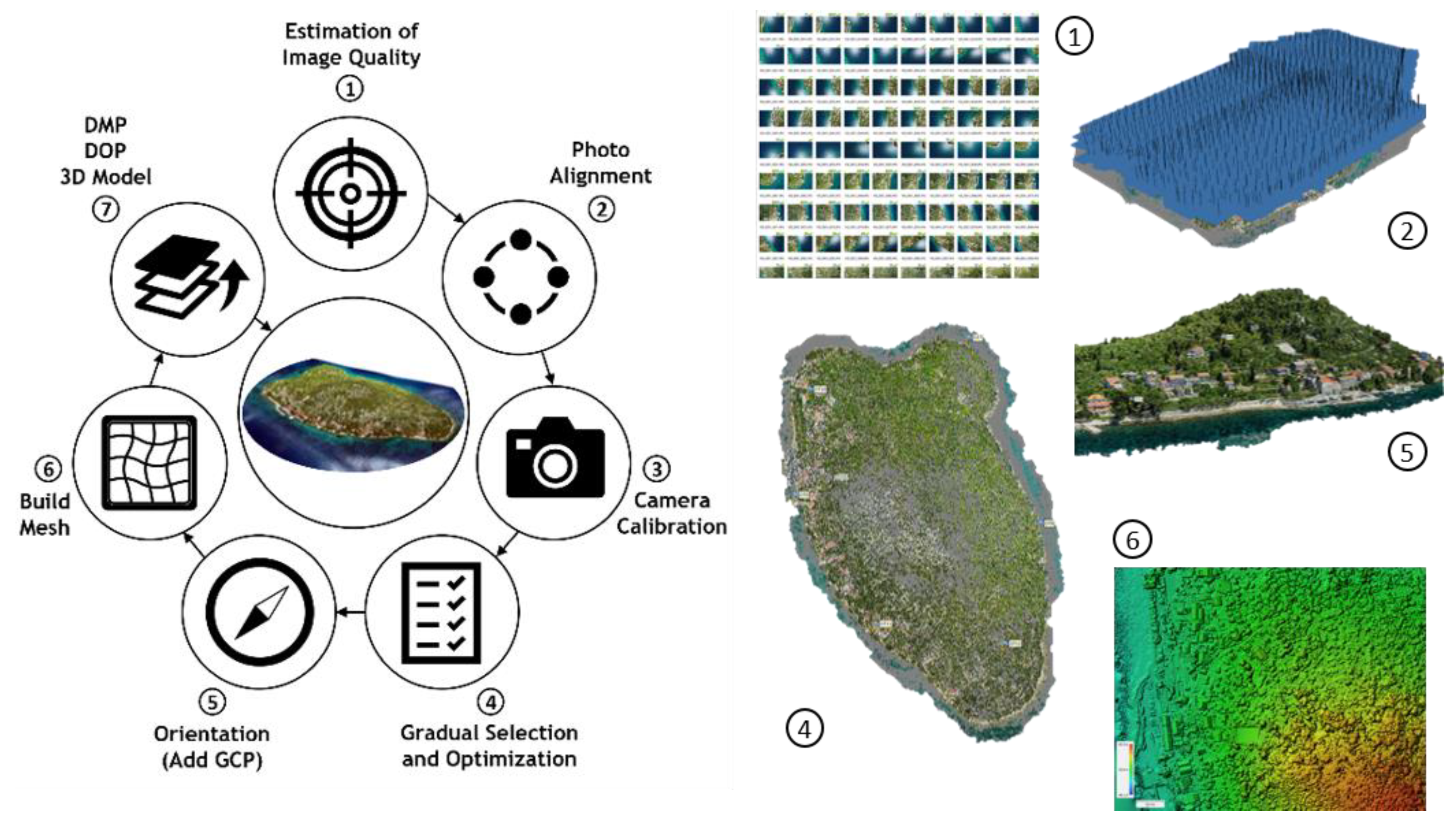
The collected UAV images were processed in Agisoft Metashape 1.5.1 (Figure 8), an advanced 3D modeling software whose main goal is to create high-quality models from photographs. This procedure, called structure from motion (SfM), operates under the same basic settings as stereoscopic photogrammetry, from overlapping photos with 3D point reconstruction. The image workflow process consisted of seven main steps (Figure 8). A total of 1199 high-quality aerial shots were collected. Over 600,000 tie points were generated whose projection error was reduced by gradual selection. The dense point cloud was created under the ultra high-quality parameter, which led to the derivation of over 600 million points for the island of Ošljak.

In-Situ Reference Data Acquisition

After DOP production, the reference (in-situ) samples were collected for validation of the 2021 LU/LC model and future research. In situ mapping was performed through several steps. First, a high-resolution DOP was created from UAV imagery. This model represents an updated template on which our location is shown while collecting control samples. Then, the Bluetooth GPS application was installed on the laptop at ArcMap and it was connected to the Stonex S10 real-time kinematic RTK GNSS receiver. This enabled precise positioning and display of our location on the updated DOP of Ošljak. It makes sampling easier because better accuracy can be achieved by immediately clicking on the specific sample (object/pixel) on the DOP and by adding the specific identification number and thematic attribute (class description) for that point. If the vegetation species of a specific sample is unknown, the Plant Net application was used to identify it (Figure 9). Finally, the collected data enabled the development and accuracy assessment of a LU/LC model of Ošljak for the year 2021.

Unfortunately, in this case, such detailed sample data cannot be used to derive the LU/LC model with multiple vegetation classes. This is because the number of classes of this LU/LC model (2021) must be consistent with the number of classes of LU/LC models derived based on greyscale HAPs. The same number of classes allows for a statistically simpler comparison. Therefore, these samples were reclassified into larger clusters (reclassify) when assessing the accuracy of the LU/LC model and while marking the samples on the segmented model. For example, samples of olives, figs, and myrtles were all classified under class (2) other bushy vegetation. Namely, since the emphasis of this research is on the spread of pine trees (more precisely Aleppo pine), other shrubby vegetation is represented as one class because it is not possible to make an accurate distinction of these species from greyscale HAPs. However, for future research, when Ošljak will be recorded with advanced multispectral cameras, these samples will certainly be useful for derivation of LU/LC model with multiple classes (n > 5) and for more detailed STC analyses. A total of 150 samples were collected.

2.2. Data Harmonization

To properly perform LUCC analysis, it was necessary to harmonize the collected multi-temporal data. In this context, data harmonization refers to the unification of all used raster data (cadastral map, HAPs, and UAV-DOP) into the same projected coordinate system and the same GSD. For the purpose of georeferencing all multi-temporal data (cadastral maps and HAPs), the newest DOP from 2021 was used as a reference. The selected coordinate system in which all raster data were georeferenced and all analyses were performed was HTRS96_Croatia_TM, i.e., the official positional reference coordinate system of HR.

The harmonization consisted of several steps. The georeferencing process is performed in the Georeferencing tool in ArcMap. To connect the known positions of the two raster dataset, links (control points—CPs) with known positions must be added. The process is such that a CP is added at a location that is clearly visible on all HAPs, as well as on the reference UAV-DOP. These locations usually include some recognizable sharp edges such as on houses, dry stone walls, or piers on the shoreline (Figure 10). A number of added control points will depend on the complexity of the used transformation. When adding CPs, special attention is paid to the correct arrangement of the points, since their spatial distribution affects the result in terms of accuracy when rectifying with transformation algorithms. However, adding more control points will not necessarily lead to better registration. If possible, control points need to be evenly distributed throughout the raster dataset, rather than concentrated in a single area. The points are added so that they are always placed opposite the previous point, in such a way that the points frame the outer dimensions of the image and move towards the central part of the photo. Swipe in the Effect Toolbar was used as an auxiliary tool to compare and track the geometric alignment. A total of 34 control points were selected for georeferencing each raster model. A total of eight transformation methods were tested: zero-order polynomial (only shift), similarity polynomial, first-order polynomial (affine), second-order polynomial, third-order polynomial, adjust, projective transformation, and spline. After discarding the six points where the largest error in the residuals occurred, the best results according to residuals and root mean square error (RMSE) in CPs were used for adjust transformation.

The value of spatial resolution was adjusted for the older HAPs. Therefore, the GSD of the models used in LUCC analysis was set to 0.5 m. For HAPs with better spatial resolution (1997–2018), and for DOP from 2021, resampling was performed in ArcMap using the bilinear resampling technique. This is used to calculate the value of each pixel by averaging (weighted for distance) the values of the surrounding 4 pixels. It is recommended for continuous data.

2.3. Derivation of the LU/LC Models

Different geographic object-based (GEOBIA) pixel-based (PB) classification algorithms, both unsupervised and supervised, enable the extraction of classes from multispectral (MS), RGB, or one-band (greyscale) images. The quality of derived classes will primarily depend on the quality of the input data and set parameters [92]. Ref. [88] have tested the applicability of the mentioned methods in the extraction of information (LU/LC classes) from greyscale HAPs [88]. The results have shown that the GEOBIA approach has an advantage over PB methods because can create a standardized set of rules that can provide efficient segmentation and classification for diverse HAPs. Therefore, a similar approach was followed in this study.

2.3.1. GEOBIA Segmentation

Unlike the traditional PB unsupervised and supervised methods, GEOBIA works on the principle of grouping pixels in objects (clusters) based on their spectral similarity. However, since classification is performed on greyscale HAPs, same limitations of this method can also occur. The first step was the segmentation of HAPs and DOP (UAV) for 2021. Segmentation was carried out in ArcGIS using the Segment MeanShift approach [93]. This delineates segments in imagery by grouping spectral, spatial, and geometric similar neighboring pixels (Figure 11).

The quality of these segments, which ultimately affect the accuracy of the LU/LC model, depends on the characteristics of the image and set parameters of spectral detail (SDe), spatial detail (SDa), and the minimum segment size (MSS). Therefore, a similar approach outlined in [88] is used, where the iterative process of setting the values of these three parameters for each raster was carried out. For each raster (n = 11) in LUCC analysis, three different combinations of parameter values were tested. This ultimately led to 33 segmented images. From the three segmented images for each raster, the best one was selected on the basis of which the classification was made. The best combination of parameter values was selected using visual interpretation (comparison of original raster and segmented image) as in [94], guided by the fact that good segmentation is a compromise between a good delineation of LU/LC classes and a reduced number of the resulting objects (elements, patches). Figure 11 gives an example of selected parameters for 1944, 2011, and 2021. It is noticeable that the spectral detail (SDe) parameter is higher for older HAPs, which is expected given their characteristics, and that MSS is set at slightly lower values (10) than recommended (20), in order to effectively map all bushy vegetation, predominantly olives.

2.3.2. Selection of LU/LC Classes

The number of classes can significantly affect the accuracy of LU/LC models and simulation models conducted in the continuation of the research. Ref. [95] states that researchers should expect about a 0.77% decrease in overall accuracy when they increase 1 LC classification class. This is especially the case if the classification is performed on an image that does not have a sufficiently detailed spectral and spatial resolution (e.g., historical greyscale image). Therefore, the classification scheme in this research consisted of six classes that are harmonized for the period from 1944 to 2021 (Figure 11). They included:

(1)

Karst bare rock;

(2)

Poorly overgrown bare karst;

(3)

Karst pastures;

(4)

Other bushy vegetation (predominantly olive);

(5)

Coniferous forest (predominantly Aleppo pine);

(6)

Urban (residential, cultural, and commercial object).

Conditionally speaking, it was assumed that a smaller number of classes would be sufficient to identify the main LUCCs and, from that, the processes that prompted these changes (deagrarianization, deruralization, afforestation, etc.) can transform the Ošljak landscape in the study period. Furthermore, the names of the classes are defined by the following examples in [3,96].

Given that there are usually different groups of pixels in class (6), and due to their spectral diversity (roofs built from tin, concrete, and tiles), they can be mixed with other classes. Following this approach [97], it was decided to delineate this class with manual vectorization from each original raster data (n = 11). Furthermore, this class was analyzed within a wider time period (1776–2021) than other LU/LC classes (1944–2021). This is because, from the acquired cadastral map (1776 and 1824), it was possible to manually vectorize only this class and make it comparable to other classes in 1944–2021 LU/LC models. Cadastral parcels derived from cadastral maps (1776, 1824, and 2020) were not recognized as a special class within the LU/LC model. They were studied as a separate element, with the aim of monitoring land parceling among landowners, as well as the impact of terrain morphometry on their geometry (location and shape).

2.3.3. Adding Training Samples

This refers to the process of collecting training samples and verifying them. Training samples were collected for the defined six classes on each segmented image. This was achieved in ArcMap using the Image Classification tool and Select Segment option. Due to the reduced spectral and spatial quality of HAPs, a larger number of training samples was selected on the whole surface of Ošljak. Around 1000 training samples were selected for each segmented image. The addition of samples for class (5) was added based on assumptions that these trees are darker, have a higher height and a shadow of ground, and occur in larger segments than samples for class Other bushy vegetation. This vegetation usually has a lower height, has a more rounded, and grows more isolated, i.e., the distance is bigger between them due to the planting plan. This assumption is based on information received from the local population. It also overlays the acquired HAPs and DOP and spots vegetation patterns. A similar approach was adopted by [88].

2.3.4. Classification of Segmented Images

The next step involved the classification of segmented images. Segmented images were classified using the support vector machine (SVM) classification algorithm. This algorithm was chosen because it is the most commonly used classification algorithm for analyzing different imagery [98], and numerous research [92,99,100] has shown that it is very accurate in identifying vegetation forms within LU/LC classes. It should be noted that testing the accuracy of classification algorithms in the derivation of LU/LC models on greyscale HAPs, through a wide range of metrics, requires special and separate research. Therefore, this will be explored in our future work. After classification, LU/LC models were converted from a raster to a vector format in order to calculate defined environmental indicators which are explained in the following section.

2.3.5. Accuracy Assessment of LU/LC Models

Accuracy assessment is regarded as an important part of the processing of various remote sensing data [101]. The accuracy assessment of derived LU/LC models (n = 11) was determined using the contingency matrix (confusion matrix). This method contains specific metrics, such as user accuracy (UA) (type error 1 or false positive), producer’s accuracy (PA) (type error 2 or false negative), overall accuracy (OA), and Kappa coefficient (K) (which describes the quality of the performed LU/LC models). The meaning of these metrics and their formulas are available in numerous LU/LC studies. The accuracy assessment process was carried out in ArcMap using the Accuracy Assessment Point tool which generated around 300 points/samples for each LU/LC model. The sampling strategy was stratified random, whereby points are randomly distributed within each class, and each class has a number of points proportional to its relative area (Figure 12).

The values of PA, UA, OA, and K were then calculated using the Create Confusion Matrix tool within ArcGIS based on the formulas below:

$$\mathrm{P}\mathrm{A}i=\frac{p_{ii}}{p_{+i}}$$

(1)

$$\mathrm{U}\mathrm{A}i=\frac{p_{ii}}{p_{i+}}$$

(2)

$$\mathrm{O}\mathrm{A}={{\displaystyle \sum }}_{i=1}^m{p}_{ii}$$

(3)

where $p_{ii}$—the major diagonal element for class i; $p_{+i}$—the total number of observations in column i (bottom margin); $p_{i+}$—the total number of observations in row i (right margin); and m—the number of rows and columns in the error matrix.

PA, UA, and OA values can vary between 0 and 1. A higher value represents higher accuracy. The formula for the Kappa coefficient (K) is calculated:

$$\mathrm{K}=\frac{M{{\displaystyle \sum }}_{i=1}^{r}xii-{{\displaystyle \sum }}_{i=1}^r{x}_i+x_{i+i}}{M^2-{{\displaystyle \sum }}_{i=1}^r{x}_i+x_{i+i}}$$

(4)

where r—the number of rows in the confusion matrix; x_ii—the number of samples in row (i) and column (i) (i.e., diagonal elements); and M—the total number of samples.

K values can vary between −1 and +1. Values < 0 represent poor; 0–0.2 slight; 0.21–0.4 fair; 0.41–0.6 moderate; 0.61–0.8 substantial; and 0.81–1 represent an almost perfect overlap of reference and classified objects.

Each generated point received a ground truth and classification attribute (from the derived LU/LC model). However, since we do not have better data to assess the accuracy of LU/LC models derived from HAPs with a spatial resolution of 0.5 m, ground truth data were estimated from these raw images, i.e., images before the classification, using the insights we gained in talking to the locals. It should be noted that this is a fairly common problem in LUCC analysis since the most common LU/LC models are validated through field surveys. However, in this research, this was conducted for the 2021 LU/LC model. Therefore, the possibility of error was reduced to a minimum because the maximum trusted data source at our disposal was used during the derivation of historical LU/LCs models. All LU/LC models had a Kappa coefficient greater than 0.6 and an overall accuracy greater than 0.65. The black and white (greyscale) HAPs had slightly worse accuracy compared to RGB imagery. The biggest errors were, as expected, in determining the classes of karst pastures and poorly overgrown bare karst.

Table 3. Example of confusion matrix table generated for 2011, 1977 and 1944 LU/LC models.

Confusion Matrix LU/LC 2011
CLASS_ID	1	2	3	4	5	6	TOTAL	U_ACC.	KAPPA
1	71	3	4	3	7	0	88	0.81	-
2	5	40	12	1	1	0	59	0.68	-
3	2	0	22	3	0	0	27	0.81	-
4	0	1	0	25	0	0	26	0.96	-
5	5	2	2	0	81	0	90	0.90	-
6	0	0	0	0	0	10	10	1	-
TOTAL	83	46	40	32	89	10	300	-	-
P_ACCU.	0.85	0.87	0.55	0.78	0.91	1	0	0.83	-
KAPPA	-	-	-	-	-	-	-	-	0.78
Confusion Matrix LU/LC 1944
CLASS_ID	1	2	3	4	5	6	TOTAL	U_ACC.	KAPPA
1	66	9	0	1	2	0	78	0.85	-
2	12	117	8	3	0	0	140	0.84	-
3	0	6	39	12	0	0	57	0.68	-
4	0	0	3	17	0	0	20	0.85	-
5	0	0	0	0	10	0	10	1	-
6	0	0	0	0	0	10	10	1	-
TOTAL	78	132	50	33	12	10	315	0	-
P_ACCU.	0.85	0,89	0.78	0.51	0.83	1	0	0.82	-
KAPPA	-	-	-	-	-	-	-	-	0.75
Confusion Matrix LU/LC 1977
CLASS_ID	1	2	3	4	5	6	TOTAL	U_ACC.	KAPPA
1	74	8	0	0	6	0	88	0.85	-
2	0	97	15	4	0	0	116	0.84	-
3	0	5	16	5	0	0	26	0.62	-
4	0	3	3	12	0	0	18	0.67	-
5	4	0	0	0	44	0	48	0.92	-
6	0	0	0	0	0	10	10	1	-
TOTAL	78	113	34	21	50	10	306	0	-
P_ACCU.	0.95	0.86	0.47	0.57	0.88	1		0.83	-
KAPPA	-	-	-	-	-	-	-	-	0.77

ID 1 = other bushy vegetation; ID 2 = karst pastures; ID 3 = poorly overgrown bare karst; ID 4 = bare karst; ID 5 = coniferous forest; ID 6 = urban.

contains an example of the confusion matrix for the LU/LC model of 2011, 1977, and 1944. The urban class had the highest UA and PA out of all the LU/LC models. The reason for this is explained in Section 2.3.2. Namely, due to it spectral diversity, following the approach [97], the decision was made to delineate this class with manual vectorization from each original raster data.

2.4. Selection of the Ecological Indicators (EI)

Improvements in GST have advanced our ability to quantify LU/LC details and landscape configuration. Different natural and anthropogenic changes in landscapes over time have raised concern in managing protected areas. In response to this, decision-makers, scientists, and conservationists are constantly developing systems composed of metrics in order to monitor the quality of landscape/landscape conditions or their “vital signs” [102]. It is beyond the scope of this research to review and use a wide spectrum of chemical, biotic, and physical indicators since the characteristics of our multi-data cannot support this, and there is already a comprehensive review of the literature on this topic [103]. Often, environmental and ecological terms are often used interchangeably, although ecological indicators are actually a sub-set of environmental indicators. Sometimes, the metrics of the landscape structure are mentioned in this context. Therefore, we analyzed Ošljak LC/LU changes by applying a selected set of metrics that can be regarded as primary environmental indicators.

For specific indicators, zonal level (hexagonal grid) calculation was used rather than the focus area defined by the data set. The ZonalMetrics toolbox was used for this approach [104], which enables direct analysis of user-defined vectors, i.e., a set of available landscape metrics, as well as the creation of specific user-defined zones (pies, hexagon). Zones were created using the Create hexagons tool. Since the size of the hexagon was based on a user-defined height parameter, each hexagon had an area of 1000 m². This enabled more precise monitoring of changes in selected classes within the studied landscape. Therefore, at the zonal level, the following indicators were used: (1) Shannon’s diversity index (SHDI) which belongs to the group of DIVERSITY metrics; and (2) the largest patch index (LPI) with (3) the percentage of zone (PZONE) which belongs to the group of AREA metrics (

Table 4. List of metrics used in LUCC analysis.

Abbreviation	Full Name	Level of Analysis	Definition
SHDI	Shannon’s diversity index	Statistical zone	the proportional abundance of each patch type
LPI	Largest patch index	Statistical zone	looks for the patch covering the largest area within the statistical zone
PZONE	Percentage of zone	Statistical zone	% of the area of the corresponding class within the statistical zone
FE	Forest extent	Ošljak landscape	total extent (ha, km2, or m2) of forest within landscape
FG	Forest gain	Ošljak landscape	transformation from an unforested to a forest class
UE	Urban extent	Ošljak landscape	total extent (ha, km2, or m2) of urban within landscape
UG	Urban gain	Ošljak landscape	transformation from n natural to an urban class
PAUFC	Percentage of area under forest cover	Ošljak landscape	% of the forest within the landscape
PAUUC	Percentage of area under urban cover	Ošljak landscape	% of the urban within the landscape

).

Shannon’s Diversity Index (SHDI) [105]

$$SHDI=-{{\displaystyle \sum }}_{i=1}^m\left(p_i\ast \ln p_i\right)$$

(5)

where $p_i$ = the proportion of the statistical zone area occupied by patch type I and m = the total number of patch types

This is the most popular diversity index because it represents the amount of “information” per patch. The absolute magnitude of this indicator is not particularly meaningful; therefore, it is often used as a relative metric in comparison of the same landscape over a period of time [106]. The minimum value of SHDI is 0, and there is no upper limit. SHDI is 0 when the landscape contains only one patch (i.e., no diversity). The value increases as the number of different patch types (i.e., patch richness) increases and/or the proportional distribution of the area among patch types becomes more equitable [107].

Largest Patch Index (LPI) [106]

$$LPI=\left(\frac{n_i}{A}\right) \ast 100$$

(6)

where $n_i$ = the area of the specific LC class and A = the total area of the statistical zone.

LPI shows which patch of a specific class dominates within a predefined zone (in this case hexagon). In other words, it looks for the path covering the largest area within the statistical zone (hexagon). This metric is very similar to the PZONE in the calculation context, but differs in display mode. Namely, after the calculation, it is not expressed as a percentage, rather as categorical data where each zone receives a thematic attribute or the name of the class whose element dominates it, i.e., the highest percentage of area.

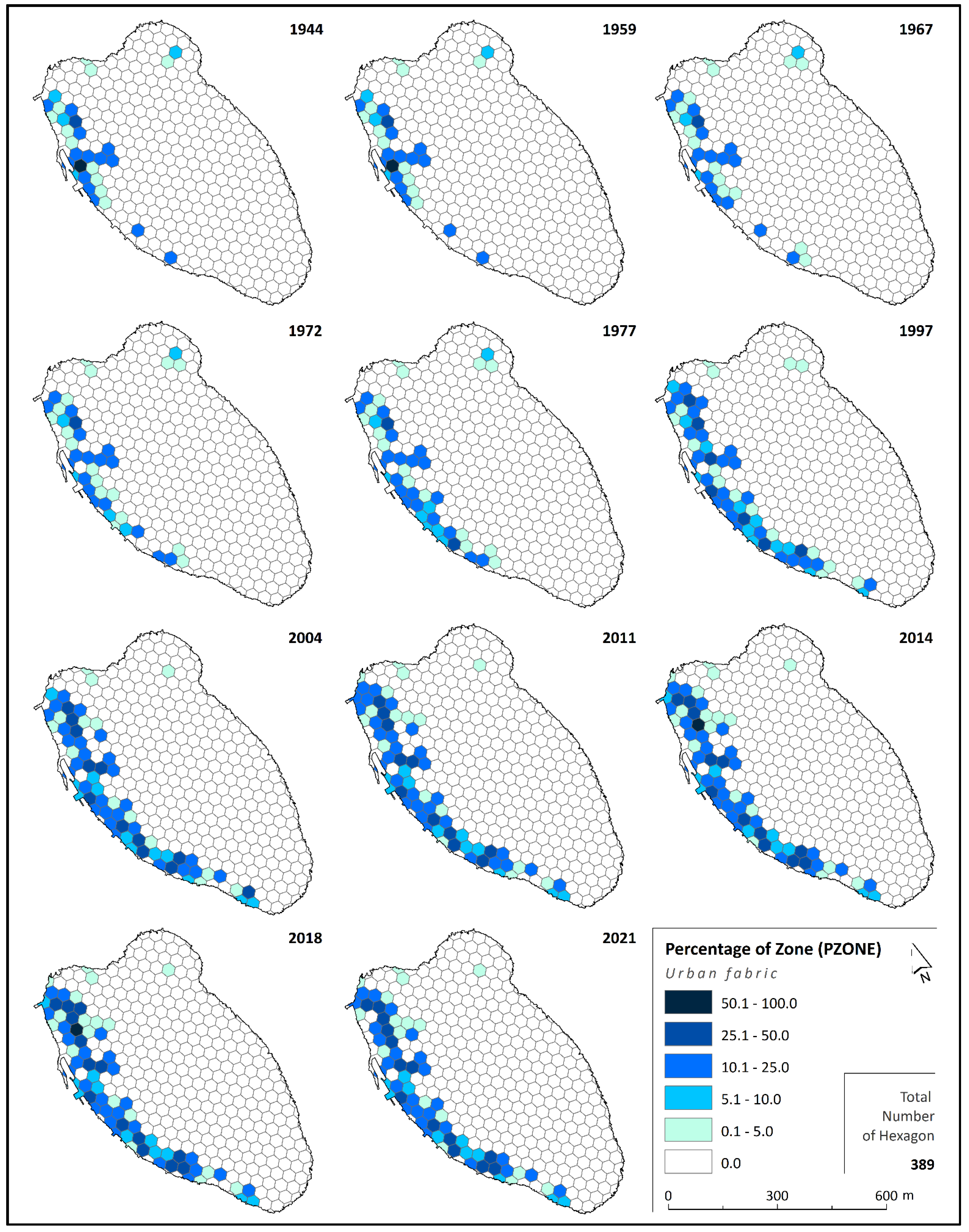
Percentage of Zone (PZONE) [104]

$$PZONE=\left(\frac{CA}{ZA}\right) \ast 100$$

(7)

where $CA$ = the total area of the corresponding patches of specific class within the statistical zone and $ZA$ = the total area of the statistical zone.

The PZONE value can vary between 0 and 100%. The PZONE is 100% when the entire landscape (in this case statistical zone) consists of a single patch of the specific class [106].

Furthermore, the following indicators were used which were not derived within the statistical zones (hexagons), i.e., they were generated for the whole Ošljak within a specific year (Table 4). They, following the examples by [108] and (UNSD) handbook [109] include:

• Forest extent (FE);
• Forest gain (FG);
• Percentage of area under forest cover (PAUFC).

Variations on these examples were made by the addition of:

• Urban extent (UE);
• Urban gain (UG);
• Percentage of area under urban cover (PAUUC).

The extent indicators aim to monitor the total area of forest (or urban) within specific landscapes. The gain gives insight into the data about the total land area that has transitioned from an unforested to a forested state within a specific period, or for another example from a natural to an urban state within a specific period. Formulas for these indicators are very simple. The extent indicator is calculated as the sum of all patches of the forest or urban classes for a specific area in a specific period. The gain indicator is calculated as the difference in the total area of the forest or urban class between the two time periods. The percentage indicator is calculated as the division of the total area of a specific class (forest or urban) with the total area of the studied landscape.

2.5. Simulation Modeling

Simulation modeling is a popular method of LU/LC model prediction. The classification scheme contains four classes. Namely, the other bushy vegetation, karst pastures, and poorly overgrown bare karst classes are reclassified into one class because the accuracy of simulation modeling is very class-dependent. The probability of error increases exponentially by introducing new classes [110]. Furthermore, preliminary analyses show that the use of the initial six classes of LU/LC will not give an accurate simulation model; therefore, the reclassification process has to be conducted.

The simulation modeling was conducted into Modules for Land Use Change Evaluation (MOLUSCE), i.e., a tool that is a plugin of QGIS. More precisely, the QGIS 2.4.0 version was used. The simulation integrated in MOLUSCE was carried out in the following steps:

(1)

Input—LU/LC models (initial and final) and explanatory variables or spatial variables were added, and explanatory variables (digital terrain model, slope, aspect, distance from a road, distance from dry stones, and curvature) were used;

(2)

Evaluation correlation—where the correlation between variables was checked;

(3)

Area change—a LU/LC change map was produced;

(4)

Transitional potential modelling—transition potential maps were derived, and an artificial neural network (ANN) was used to model the transition potential of LU/LC (Figure 13).

Then, (5) in cellular automata simulation, simulated LU/LC maps and transition potential maps were generated.

In the final (6) step, the simulated model was validated with our reference LU/LC model. Here, standard kappa statistics were produced.

In order to perform the simulation model of Aleppo pine expansion for 2025, it was necessary to use three LU/LC models (2004—initial, 2011—final, and 2018—reference). The number of iterations in the cellular automata simulation step was set to 2, in order to obtain a time interval of 14 years and a simulation model for 2025.

3. Results

3.1. LUCC Analysis (1944–2021)

Following conducted methodology on Figure 14, derived LU/LC models for Ošljak Island in the time period of 1944–2021 are shown.

By only visual interpretation of derived LU/LC models, two significant processes that took place in the studied period can be clearly observed. The first is the significant expansion of coniferous forests, dominated by Aleppo pine, which occurred on the central (highest part of the island), the northern, eastern, and southeastern part of the island, and following the coast. The second is the urban sprawl of residential and commercial objects on the west side of the island that faces the settlement of Preko on the island of Ugljan (

Table 5. LUCCs results for the 1944–2021 time period.

	Area (ha)	Area (ha)	Difference (ha)
Class	1944	2021	1944–2021
Poorly overgrown bare karst	2.33	1.71	−0.62
Bare karst	6.34	1.52	−4.81
Dry karst pastures	15.60	4.68	−10.92
Other bushy vegetation	8.72	12.84	+4.12
Coniferous forest	0.25	11.74	+11.49
Urban	0.31	1.06	+0.75
SUM	33.54	33.54

).

The largest area in the LU/LC model from 1944 has the class karst pastures (15.6 ha) and other bushy vegetation (8.72) (Table 5). The following then includes larger cultivated species (olive, vines, figs) and shrubs. This is evident from the length of dry stones (27,841 m) in that period, which was determined by manual vectorization and historical cadastral maps. This network of dry stones covered the entire island, delineating the small patches of shallow arable land. Furthermore, a total area of 8.66 ha for bare karst and poorly overgrown karst confirms the presence of dry stones (Table 5). The LU/LC model from 2021 showed that the landscape changed significantly in the 77 year period (Figure 14). Field surveys and conversations with the local elderly population also confirmed this. There are almost no cultivated areas, and they are being replaced by Mediterranean macchia and the spread of invasive vegetation, i.e., Aleppo pine (Table 5). The reasons for this landscape transformation are explained in detail in the Discussion chapter. Therefore, if a more detailed comparison is made on the interval LU/LC models (1944–2021), the following dominant changes in the Ošljak landscape are noticeable: (1) a large increase in the extent of a coniferous forest; (2) an increase in the extent of urban class, which does not cover a large area (Figure 15), but is spatially noticeable on LU/LC models (Figure 15); (3) a decrease in bare karst (predominantly dry stones), karst pastures, and poorly overgrown bare karst associated with extensive agriculture and livestock (Figure 15).

3.2. Environmental Indicators

3.2.1. Statistical Zone (SHDI, LPI and PZONE)

In the following models, which included SHDI, LPI, and PZONE models for the statistical zone of Ošljak for each LU/LC model, the dominant spread of the Aleppo pine and urban is even more visible (Supplementary Materials). There is a noticeable decrease in the value of SHDI in those areas where the Aleppo pine has spread (Figure 16). A lower SHDI value indicates the smaller diversity within the specific landscape. Therefore, zero indicates that there is only one class within the study area or zone. LU/LC from the 1944 model did not have a single zone (hexagon), whereby the only class was coniferous forest, while the LU/LC model from 2021 had four zones. The difference is even more noticeable within the first class (0–0.35) of the derived SHDI model. This class is shown bright red on Figure 16. In 2021, 51 out of 389 hexagons (15.2%) belonged to the first class; in 1997, 26 out of 389 hexagons (6.67%) belonged to the first class; and in 1994, only 6 out of 389 hexagons (1.5%) belonged to the first class. These values are very important indicators of possible disturbance in the Ošljak landscape. Namely, some studies have shown that there is a reduction in biodiversity from 20 to 50% in areas under the complete dominance of Aleppo pine [111,112].

The dominance of Aleppo pine within the defined statistical zones of the Ošljak landscape is effectively shown by the LPI (Figure 17) model. In 1944, Aleppo pine was the dominant class within only one hexagon of 389 (0.25%). Then, that number gradually increases; it was 75 (19.28%) in 1977, and was dominant in 167 hexagons (42.9%) in 2021, i.e., almost half of the island.

PZONE values (Figure 18 and Figure 19) provide a more detailed insight into the process of afforestation of Aleppo pine and urban sprawl. The advantage of this type of visualization is the possibility of classifying the distribution of specific classes according to selected categories. For example, in the case of Aleppo pine, classification can be used, as suggested in [63]: (a) complete dominance of Aleppo pine; (b) larger groups of Aleppo pine trees; and (c) sporadic occurrence of Aleppo pine trees.

3.2.2. Extent, Gain, and %

Table 6. Six indicators (FE, FG, PAUFC, UE, UG, and PAUUC) for (1994–2021).

Time Period	Forest Extent (FE)/ha	Forest Gain (FG)/ha	PAUFC %	Time Period	Urban Extent (EU)/m2	Urban Gain (UG)	PAUUC %
	no data	no data	no data	1776–1824	746.4	746.4
–1944	0.249	-	0.74	1825–1944	3064.2	2317.8	0.22
1945–1959	0.507	0.258	1.51	1945–1959	3064.2	-	0.91
1960–1967	4.139	1.938	7.29	1960–1967	3721.6	657.3	1.11
1968–1972	2.446	1.694	12.34	1968–1972	4002.5	280.9	1.19
1973–1977	5.342	1.203	15.93	1973–1977	4754.9	752.3	1.42
1978–1997	9.002	3.659	26.84	1978–1997	7804.3	3049.3	2.33
1998–2004	10.021	1.019	29.88	1998–2004	8834.0	1029.7	2.64
2005–2011	10.106	0.085	30.13	2005–2011	9251.0	416.9	2.76
2012–2014	10.741	0.635	32.03	2012–2014	9369.6	118.6	2.80
2014–2018	11.338	0.597	33.81	2014–2018	9440.8	71.1	2.82
2018–2021	11.736	0.398	33.81	2018–2021	9532.2	91.3	2.85

shows summary results for the other six indicators used in the LUCC analysis. By comparing the current state of densely overgrown areas of the Ošljak landscape in 2021 with those before afforestation in the middle of the 20th century, we can say that the coniferous forest (predominantly Aleppo pine) has expanded intensively to an area of 11.736 ha (39.8%) in more than 70 years, i.e., its area increased by ×47.

Figure 20 summarizes the data for forest gain (ha) through the years visualized using an Excel tree map. As expected, the highest value of forest gain was measured for the longest period of time between the two HAPs (1977–1997). In that period (20 years), coniferous forest has spread to 3.66 ha. The smallest FG was measured in the period from 2005 to 2011, only 0.085 ha. Furthermore, it can be concluded that the rate of coniferous forest expansion does not show significant signs of deceleration. Namely, in the twenty-year period of 1977–1997, the coniferous forest expanded to mentioned 3.66 ha, and increased by 2.35 ha over the next twenty-year period (1998–2018).

Figure 21 shows a number of built-in residential and commercial objects time periods between acquired sources. By 1944, and the first HAP, 44 facilities had been built on the island. Namely, from the middle of the 18th century until 1931, the number of inhabitants increased constantly (Table 1), which encouraged a gradual increase in the construction of new housing units, more intensive use of arable land, and the construction of a primary school. Depopulation begins in the inter-census period from 1931 to 1948. At that time, the events on Ošljak were significantly influenced by the Second World War when Italian fascist authorities set up a concentration camp on the island.

3.2.3. Cadastral Analysis

Gradual urban expansion (Figure 19 and Figure 21) and demographic development (Table 1) were accompanied by the fragmentation of arable land on Ošljak (Figure 22A–C). A map of Ošljak (Pianta del Scoglio Osgliach) from 17 October 1776, i.e., the oldest source used in the analysis, shows 20 cadastral parcels. Furthermore, on pages IV and V of the Preko Cadastral plan from 1824, 140 cadastral parcels were identified (Figure 22A). The fragmentation of agricultural land continued at a time when the island was owned by the Jurić family and then by the Nakić family [113,114]. Then, the local residents bought the island from the Nakić family and became the owners of those plots. Since then, the fragmentation of property and parcels has improved significantly; therefore, in the 2020 cadastral map, 1136 cadastral parcels were identified on the island, with an average size of 295.2 m² (Figure 22C).

3.3. Simulation Modeling

The 2018 LU/LC model generated a satisfactory level of accuracy. The overall kappa value was 0.67, with a correctness percentage of 74.1%. The ANN-multilayer perception model was then used to forecast LULC for 2025. The results of the simulation model showing the dynamics of the Aleppo pine class expand on Ošljak using the PZONE indicator (Figure 23). The simulation model indicates that a continuation of forest expansion will occur. It will be on those locations, i.e., statistical zones, where Aleppo pine is recognized as a dominant patch, or have a higher PZONE within the hexagon. However, the rate of expansion should be somewhat slower if other analyzed periods are observed (Table 6). If the FG is calculated compared to the 2021 data, the Aleppo pine is expected to increase by an additional 0.153 ha on the Ošljak island by 2025.

4. Discussion

In this chapter, the potential causes of detected LU/LC changes are explained in detail.

Afforestation (Invasion of Aleppo Pine).

Increase in Coniferous Forest.

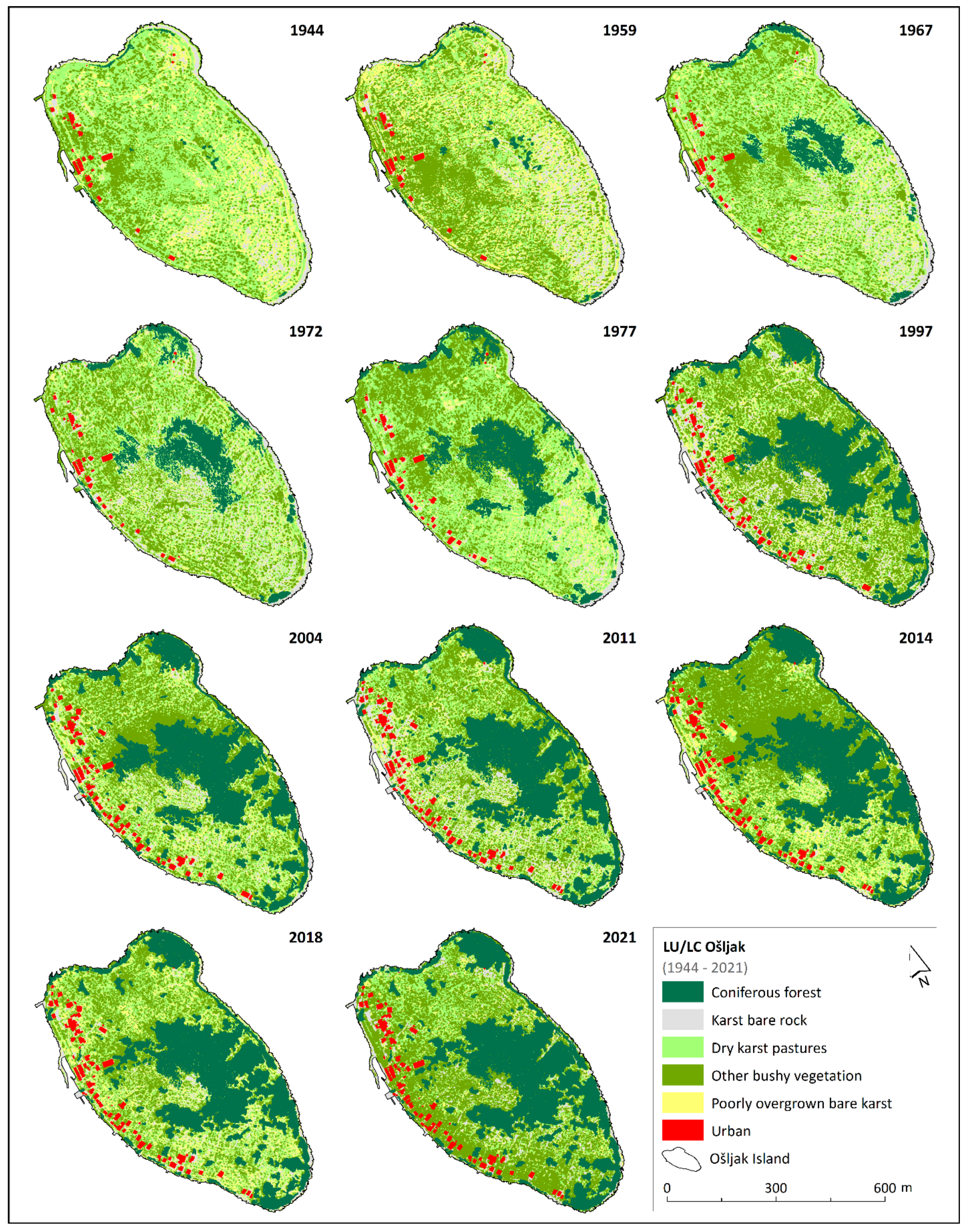
LUCC analysis has shown that the key factor in the LUCCs of the Ošljak landscape is the spread of coniferous forests in which Aleppo pine predominates (Figure 23). This has led to direct changes in the structure of the landscape, as indicated by derived indicators (Figure 15, Figure 16, Figure 17 and Figure 18). In this case, Aleppo pine, considered as the most flammable species in the Mediterranean [115], given that it is an allochthonous species, can be classified in the category of invasive vegetation. Namely, the large quantities of Aleppo pine in small areas, such as Ošljak, can lead to moisture and nutrient depletion from the soil, reducing the chances for the survival of other species [116].

The beginning of this change was due to afforestation [63,117], which marked the beginning of a new era at the Croatian coast in the 18th century. At that time, several species that met the prescribed purpose were selected for afforestation; however, in the end, Aleppo pine prevailed [63]. The Aleppo pine on Ošljak Island was planted between the two World Wars [118]. After afforestation, the Aleppo pine gradually spread (Figure 24). Ošljak is not the only Croatian island facing this problem. Ref [63] cites several studies which mention the islands of Žirje and Zlarin, where the spread of Aleppo pines has progressed significantly by “eating” abandoned vineyards and olive groves. Now, these islands are almost completely covered with Aleppo pine with (66%) and (74%). Ref. [115] mentions Mljet and Kornati national parks (NPs), where Aleppo pine has expanded. However, it is necessary to point out that the spread of Aleppo pines also played a somewhat positive role for Ošljak. The general useful functions of it include the protection of soil from erosion by water and wind, balancing water relations in the landscape and providing space for rest and recreation. Furthermore, due to the shade created by their canopy and the aromatic scent of pine needles, tourists visit Ošljak as a bathing destination during the summer months. Excursion trails framed by evergreen vegetation are also an attractive factor, especially those along the coast.

Deagrarianization and Secondary Succession.

Decrease in Karst pastures, Bare karst and oorley overgrown karst.

Ref. [75] has analyzed the process of deagrarianization across Croatian (small and distant) islands. The small and old population on the Croatian island, and in Ošljak, is abandoning traditional forms of agriculture, which is influencing changes in the island’s landscape [73,75,117]. Therefore, the Croatian islands, unlike the Mediterranean, takes on characteristics of a demographic and economically depressed area. Namely, [70] stated that the process of deagrarianization on the small Croatian islands began even before 1971 and that, even then, a more intensive development of tourism occurred. The derived data support this claim, given that more intensive construction of objects on Ošljak began in the mid-1970s (Video 2). Arable land becomes neglected and gradually overgrown. Process of secondary succession occurs, i.e., gradual overgrowth of shallow soil and pastures into bushy vegetation. Furthermore, island roads and dry stone walls are also overgrown by vegetation [115]. The spread of Aleppo pine, which become the main modifier in the landscape, has also been facilitated by the disappearance of significant agricultural activities and smaller livestock activities, as well as the depopulation process, which is explained in the following chapter.

Dry stones, popularly called stone lace, are considered a valuable heritage and are one of the identity symbols of the Mediterranean coast and islands. The inclusion of dry stone in the UNESCO list of intangible world heritage has given recognition to generations of unnamed builders from all over the Mediterranean. This cultural element of landscape tells a long struggle of coexistence between man and karst. Dry stones have multiple roles in the Mediterranean landscapes, both on other Mediterranean islands and Ošljak. They served as a physical boundary of land parceling and as a natural defense from soil erosion that follows the configuration of the terrain. This problem is beautifully described by Josip Marcelić, the then Bishop of Dubrovnik, a native of Preko, in a booklet about Preko written in 1924. He wrote: “rains almost spilled all soil into the sea little by little, only something was left on the stands by the sea and which serves the residents to plant vegetables” [114]. Due to the resolution of the LU/LCs model (0.5 m), the dry stone element was mapped by manual vectorization of 1944 HAP, when there was not so much forest on Ošljak. A total length of 27,841 m of dry stone was calculated. The dense vegetation (spreading of Coniferous forest) visible on the DOP from 2021 made it impossible to determine the exact number of dry stone walls. Therefore, we rely on data derived from LU/LC, i.e., those classes whose biophysical properties represent dry stone walls. From these data, a reduction in the amount of these areas stated in the results was determined. Thus, it can be concluded that, in the observed period, there was a decrease in the area of bare karst, and thus a possible increased threat to dry stone.

Urban Sprawl and Demographic Decline.

Increase in Urban Class.

After the demographic peak in 1931 (Table 1), the island is experiencing almost constant total depopulation. A small amount of arable soil [114], fragmentation of property (Figure 21), war, and the desire for new challenges are among the main reasons for the emigration of Ošljak residents. A large number of residents emigrated to Zadar and other Croatian cities on the wave of industrialization and urbanization after the Second World War. All of this resulted in the weakening of the biological and economic vitality of the inhabitants of Ošljak; thus, in addition to the negative migration balance, the depopulation of this island was greatly influenced by the negative natural change in the population. However, although the number of inhabitants decreases until 1991, the number of the built objects is constantly growing (Video 2). Data about the increase in the Ošljak population in recent decades (1991 and 2022) must be taken with caution. Field research, i.e., interviews with older residents, found that this number is due to the fact that a certain amount of people who live in nearby Zadar are also listed as residents of the island. This is because they have certain benefits as pensioners (free public transport; free recreational permit; fishing; treating housing units as those intended for permanent residence, not for rest and recreation, which has tax implications; etc.), while the reason for fictitious registration on the island is unknown for the listed younger residents. The reason for the constant increase in the number of objects in recent decades is the building of housing intended for rest and recreation (cottages and apartments), which has intensified as the urban class has longitudinally expanded along almost the entire western coastal facade of the island.

Transformation of the Ošljak Natural and Functional Landscape.

Thanks to the communities which are characteristic for traditional Mediterranean landscapes, Ošljak entered in the register of protected natural heritage in the category of significant landscape. However, LUCC analysis, followed with a cadastral parcel and urban sprawl analysis conducted in this research, has shown that coniferous forest (dominated with Aleppo pine) has covered many traditional landscape patterns and has become one of the most important constituent element (patch) of the modern LU/LC of Ošljak Island. Namely, Ošljak is often advertised as an example of a traditional Mediterranean landscape. However, results have shown that the natural basis of LU/LC in the studied time period, and consequently the function of the island landscape, has changed significantly.

The environmental indicators used in this study indicated the possibility of reduced biodiversity on the island and, at the same time, increased vegetation biomass; thus, there is a higher risk of fire ignition since Aleppo pine belongs to the group of pyrophytes, i.e., plants whose spread is facilitated by fires [112]. In recent decades, the coastal area of Ošljak has become a resource that is intensively valued in tourism. In addition to tourists who come and stay on Ošljak, island beaches with pebbles and slightly sloping flat rock outcrops are also visited by bathers who come from Zadar and nearby settlements on the island of Ugljan. In accordance with the identified changes, the Ošljak area has, to a greater extent, taken over the function of a space intended for rest and recreation (tourism) with a higher share of occasional users compared to permanent residents.

There is certainly room for improving measures and action plans regarding the management of this small and sensitive Mediterranean landscape. The public institution for the management of protected natural objects in Zadar County, Natura Jadera, should additionally take care of the entire island as a significant landscape. Although the island underwent a significant transformation of its natural basis in the last 70 years, marked by the loss of the original elements of the Mediterranean landscape, the management of this area must be adapted to new circumstances, but in an attempt to minimize the negative impact of detected changes (expansion of invasive Aleppo pine vegetation, further apartmentization and concreting of the coast, potential degradation, and disappearance of dry stones). Therefore, the following measures should be implemented: (a) regularly maintaining local roads while keeping the whole island as a pedestrian zone; (b) preventing destruction of dry stones due to unfavorable weather factors, overgrowing with unwanted, and/or invasive vegetation in order to maintain the characteristic appearance of traditional drywall; and (c) paying more attention to the aesthetic and functional arrangement of mules and small docks, which are built spontaneously with different materials, and often without any permission (since this is a sensitive maritime public good every intervention should be justified by a public purpose). Although an allochthonous, invasive species, Aleppo pine has certain positive factors on the island’s landscape that should not be neglected. They include protection from the wind and soil erosion by creating shade for beaches and roads, i.e., a positive impact of tourism. However, it would be beneficial (d) to limit the spread of this vegetation to the current extent so that it does not endanger the centuries-old olive trees on the island, other autochthonous vegetation forms, and dry stones. Moreover, it should be noted that the initial afforestation with Aleppo pine made great sense, due to its other positive effects. However, the continuation of its dominant expansion is in contradiction with today’s environmental policy objectives of European Union (EU) which are directed towards the preservation of Mediterranean landscapes.

5. Conclusions

In this paper, we analyzed the spatio-temporal changes (STCs) of the Ošljak island landscape, the smallest inhabited island in HR. Using the wide range of multi-temporal dataset (77 years span) and defined environmental indicators, LUCC analysis was conducted to identify the dominant process that occurred in the 77-year time period on Ošljak Island.

The detected LU/LC changes were: an increase in coniferous forest and urban, and a decrease in karst pastures, bare karst, and poorly overgrown karst classes. The results have shown that, in recent decades, Ošljak has undergone a significant landscape transformation which was manifested through; (a) a pronounced expansion of Aleppo pine; (b) deagrarianization, which led to secondary succession; and (c) urban sprawl (building of housing intended for rest and recreation), which all led to the transformation of the functional landscape.

In a 77-year span, the Aleppo pine has expanded intensively to an area of 11.736 ha (39% of the total Ošljak area). Many other Croatian islands are experiencing a similar transformation. However, the succession of invasive (Aleppo pine) and indigenous vegetation was recorded with somewhat positive and negative implications. Nevertheless, by taking into account the performed LUCC analysis and simulation modeling, it can be carefully concluded that the trend of an increasing share of Aleppo pine in the total area of Ošljak landscape will continue to grow, which could jeopardize this eco-system’s biodiversity and the characteristic Mediterranean landscape.

In accordance with the new island functions, it is necessary to develop a new management model that can ensure the sustainable, inclusive, and smart development of Ošljak. Within this research, specific guidelines for the management of this new transformed landscape new are proposed. They include (a) regularly maintaining local roads while keeping the whole island as a pedestrian zone; (b) preventing destruction of dry stones due to unfavorable weather factors, overgrowing with unwanted, and/or invasive vegetation; (c) paying more attention to the aesthetic and functional arrangement of mules and small docks, which are built spontaneously with different materials and often without any permission (since this is a sensitive maritime, public intervention should be justified by a public purpose); and (d) limiting the spread of this vegetation to the current extent so that it does not endanger the centuries-old olive trees on the island, other autochthonous vegetation forms, and dry stones.

This research provides a user-friendly methodological framework that can efficient monitor LUCCs of a smaller area in the case when geospatial data are scarce. Additionally, it gives an insight into the availability and quality of some multi-temporal data for the territory of the HR, as well as how to harmonize it and perform LUCC analysis.