
NDVI Threshold-Based Urban Green Space Mapping from Sentinel-2A at the Local Governmental Area (LGA) Level of Victoria, Australia


Abstract
:1. Introduction
- 1.
- Utilisation of high quality and publicly available low cost remote sensing data for mapping and monitoring of urban green vegetation abundance.
- 2.
- 3.
- Evaluation and selection of NDVI threshold ranges using a quantitative iterative optimal approach.
- 4.
- Development of indices and insights on the association of demography with urban green infrastructure.
2. Related Works
2.1. Index-Based Classification
2.2. Machine Learning-Based Classification
2.2.1. Traditional Machine Learning-Based Classification
2.2.2. Deep Learning-Based Classification
3. Materials
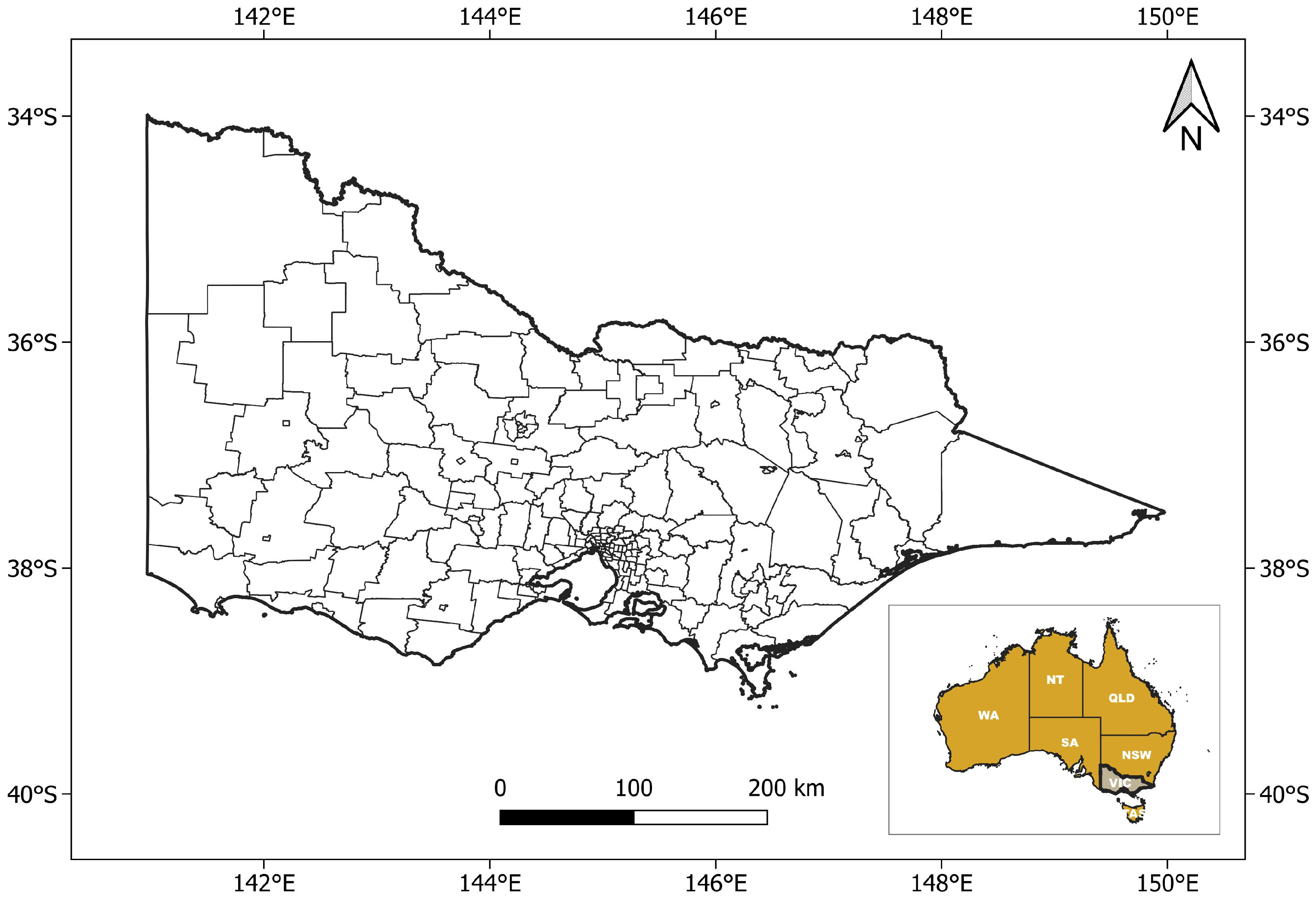
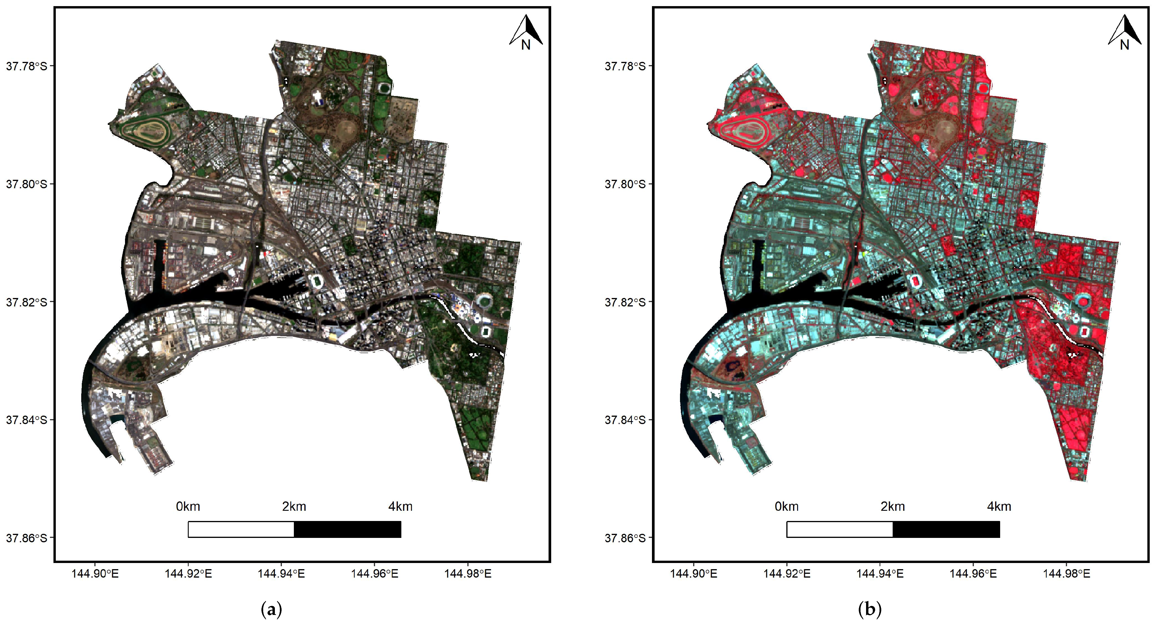
3.1. Study Area
3.2. Satellite Images: Sentinel-2A
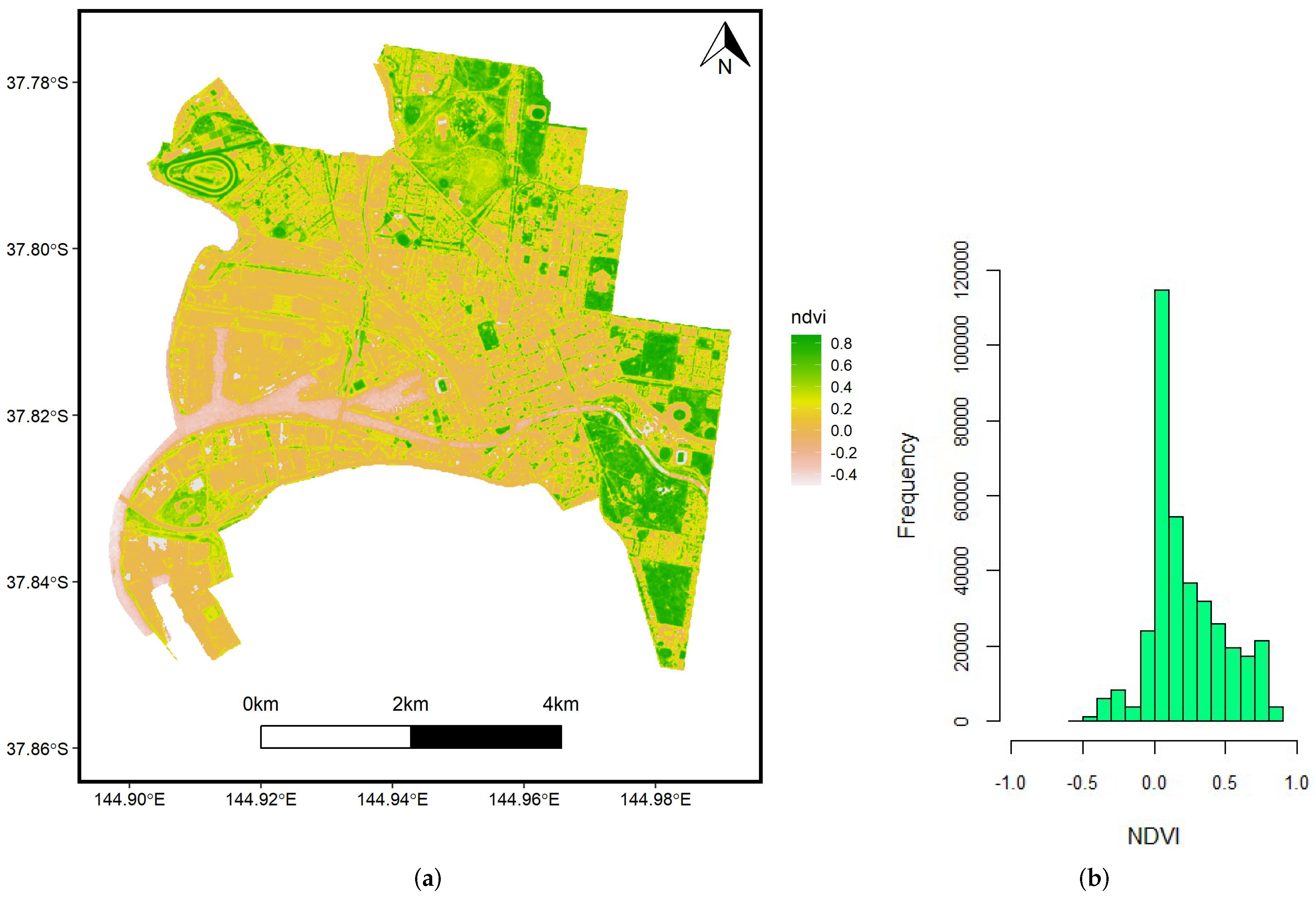
3.3. Normalized Difference Vegetation Index
3.4. Urban Green Space Index and per Capita Green Space
4. Methods
4.1. Acquisition and Pre-Processing of the Sentinel-2A Dataset
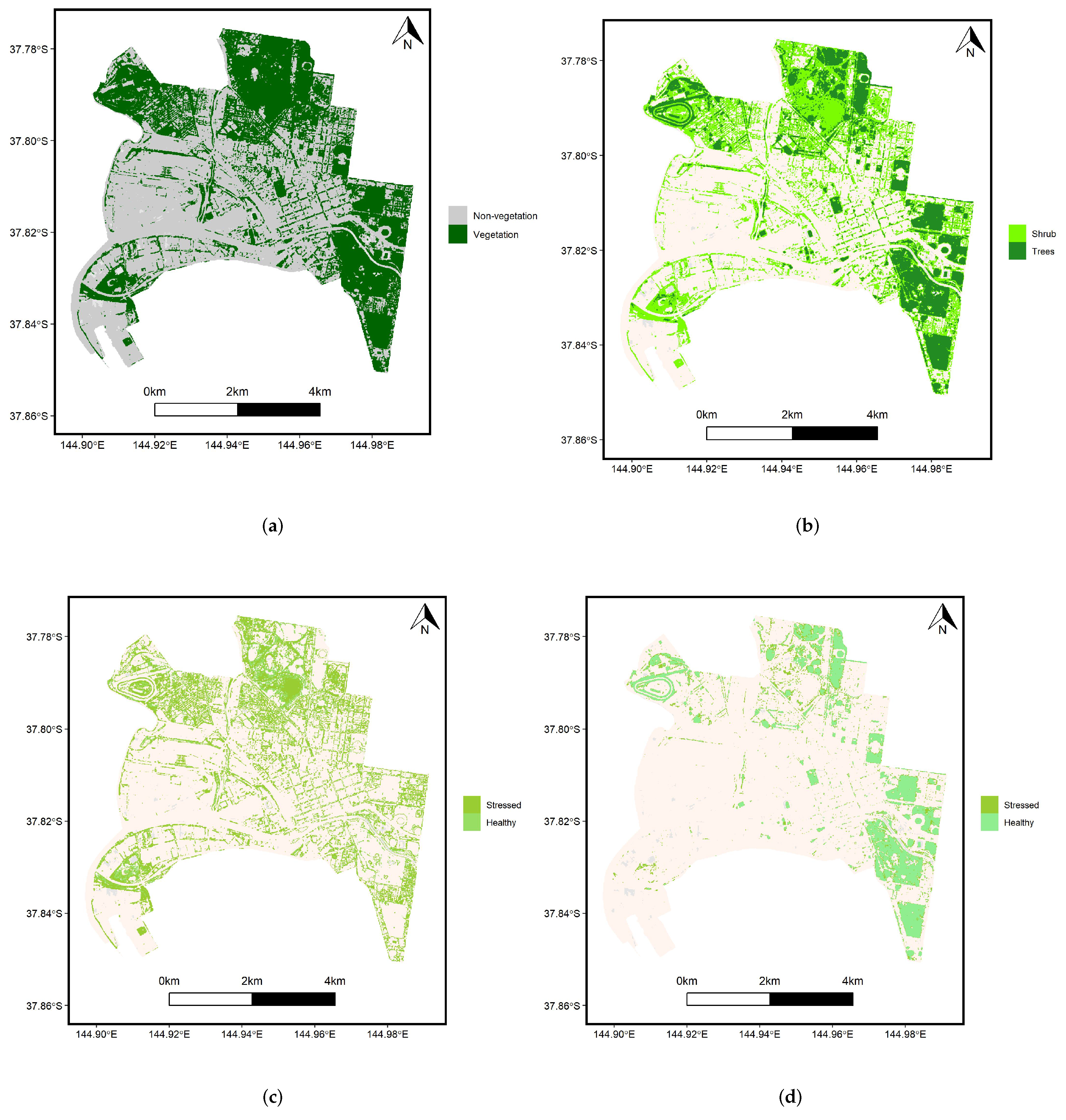
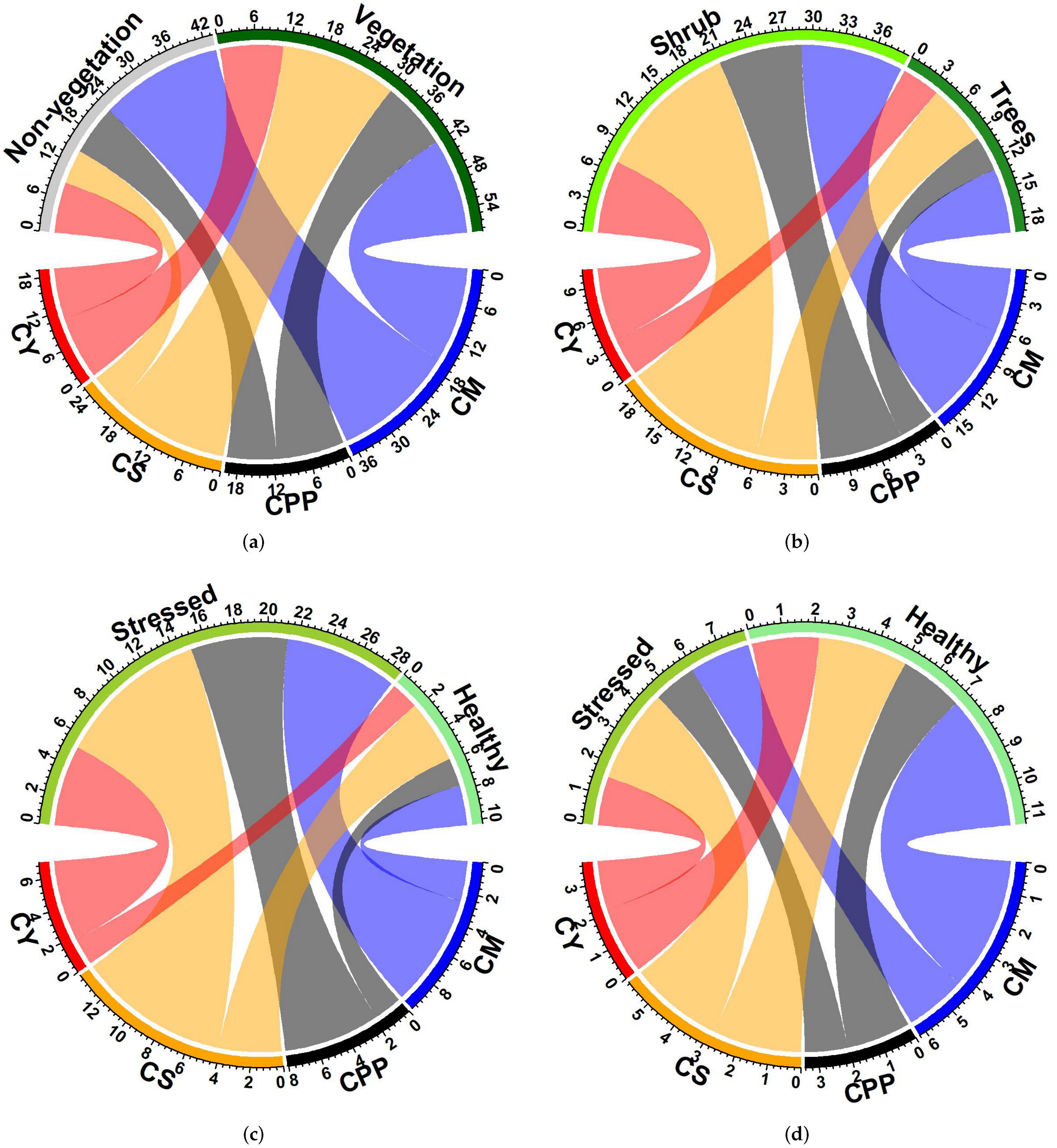
4.2. Level-1 Classification
4.3. Level-2 Classification
4.4. Level-3 Classification
4.5. Accuracy Assessment
5. Results and Discussion
5.1. Results on Various NDVI Threshold Ranges
5.2. Result of Classified Outputs
5.3. Analysis of Threshold Ranges
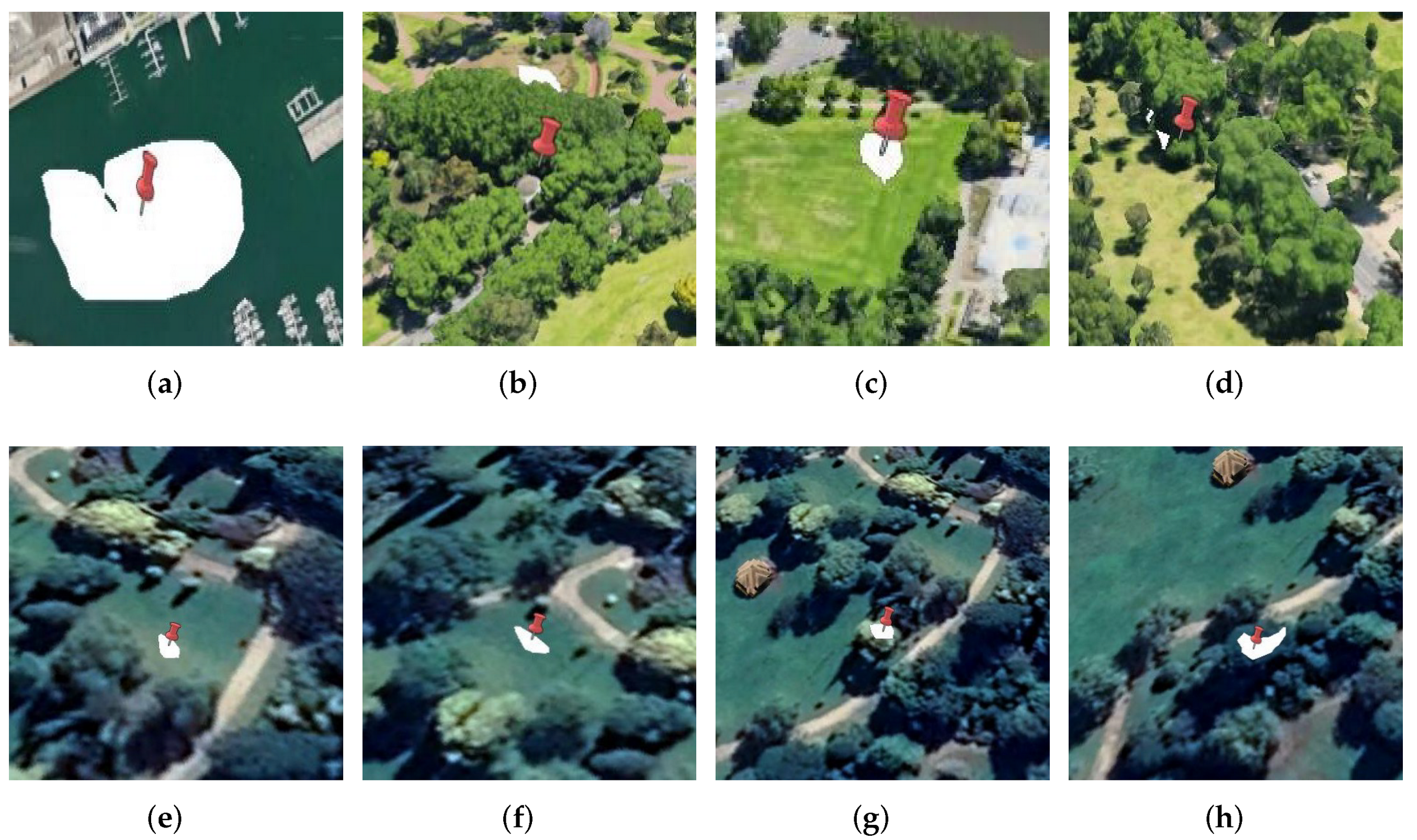
5.4. Analysis of Vegetation Distribution
5.5. Implication of Our Database in Greenprinting
5.6. Key Contributions of This Study
- 1.
- Integration of publicly available remote sensing image database for each LGA of Victoria (a total of 78 LGAs in our work) based on the Sentinel-2A products. Our database platform is readily useful for different tasks such as systematic urban spatial planning.
- 2.
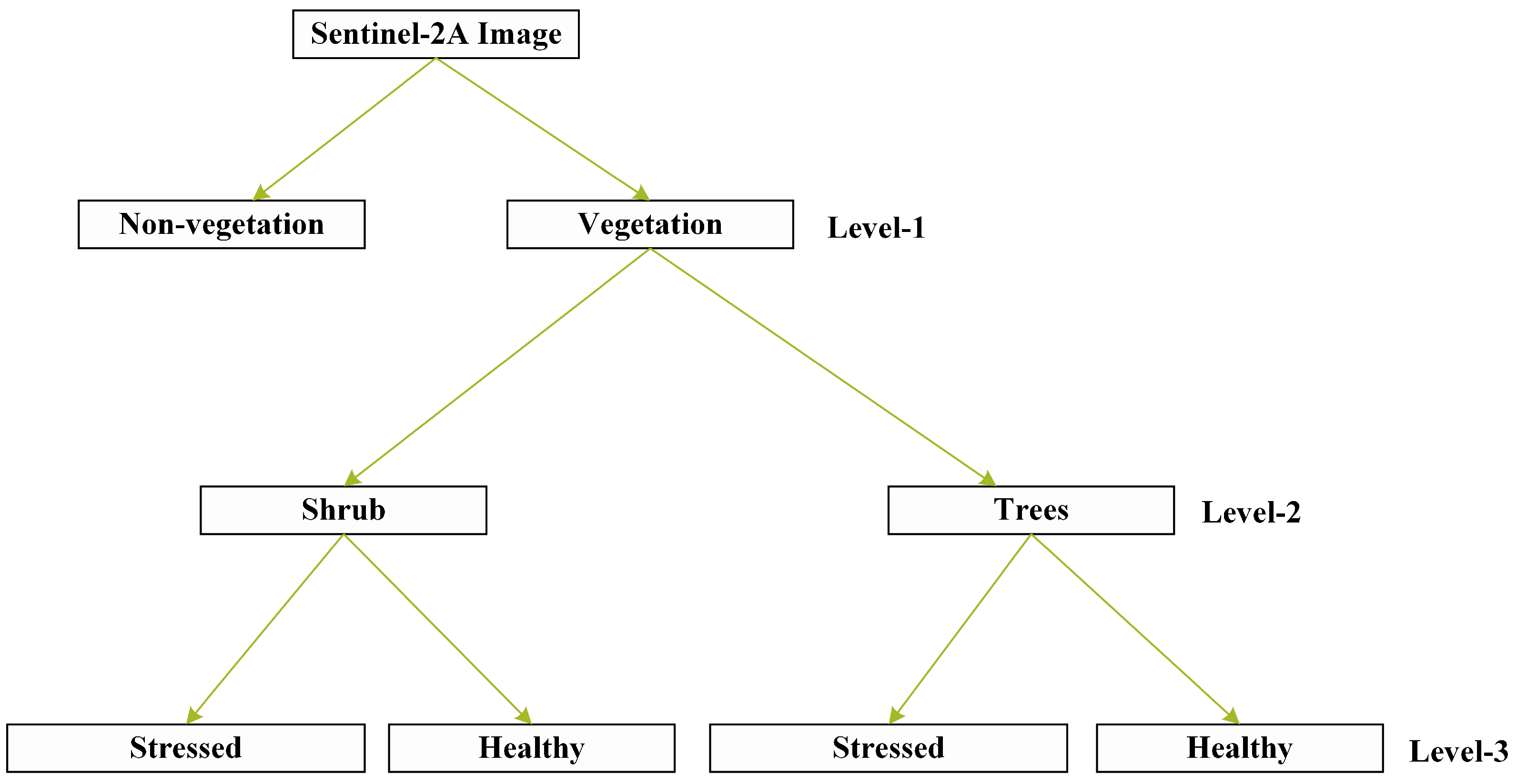
- Hierarchical mapping of urban vegetation into three levels. At the first level (Level-1), we categorise each LGA region into two classes: vegetation and non-vegetation (land). Next, at Level-2, we further categorise the vegetation regions into two sub-classes: shrub and trees. Lastly, at Level-3, both shrub and trees are further categorised into two finer groups: stressed and healthy. The classification maps of three different levels have multiple usability for different stakeholders—for example, biodiversity conservationists, urban planners, bushfire modellers, ecological modellers, and urban agriculture monitoring activities, among many others.
- 3.
- Design of experiment based on quantitative iterative optimal approach in ascertaining the NDVI threshold ranges. In doing this, we derive statistical measures such as mean precision, recall, f-score, and accuracy for evaluation purposes. In addition, then, using such metrics, we adopt the best threshold range for each hierarchy.
- 4.
- Modelling of association between demography and urban green abundance. In doing this, we compute Urban Green Space Index (UGSI) and Per Capita Green Space (PCGS) for each Local Government Area (LGA), which will eventually help in sustainability and resilience research of the cities.
5.7. Limitations of This Study and Future Potential
6. Conclusions
Supplementary Materials
Author Contributions
Funding
Institutional Review Board Statement
Informed Consent Statement
Data Availability Statement
Conflicts of Interest
| 1 | We exclude Bass Coast Shire in our work because Copernicus Open Access Hub did not allow us download the Sentinel-2A image. |
References
- Simonetti, E.; Simonetti, D.; Preatoni, D. Phenology-Based Land Cover Classification Using Landsat 8 Time Series; European Commission Joint Research Center: Ispra, Italy, 2014. [Google Scholar]
- Gorelick, N.; Hancher, M.; Dixon, M.; Ilyushchenko, S.; Thau, D.; Moore, R. Google Earth Engine: Planetary-scale geospatial analysis for everyone. Remote Sens. Environ. 2017, 202, 18–27. [Google Scholar] [CrossRef]
- Copernicus Open Access Portal. 2020. Available online: https://scihub.copernicus.eu/ (accessed on 10 September 2020).
- EO Browser. 2020. Available online: https://www.sentinel-hub.com/explore/eobrowser/ (accessed on 23 November 2020).
- Earth Explorer. 2020. Available online: https://earthexplorer.usgs.gov/ (accessed on 23 November 2020).
- El-Mezouar, C.; Taleb, N.; Kpalma, K.; Ronsin, J. A high-resolution index for vegetation extraction in IKONOS images. In Proceedings of the Remote Sensing for Agriculture, Ecosystems, and Hydrology XII, Toulouse, France, 20–22 September 2010; International Society for Optics and Photonics: Bellingham, WA, USA, 2010; Volume 7824, p. 78242A. [Google Scholar]
- Li, F.; Han, L.; Zhu, L.; Huang, Y.; Song, G. Urban Vegetation mapping based on the hj-a ndvi reconstruction. Int. Arch. Photogramm. Remote Sens. Spat. Inf. Sci. 2016, 41, 867–871. [Google Scholar] [CrossRef] [Green Version]
- Yu, F.; Price, K.; Ellis, J.; Kastens, D. Satellite observations of the seasonal vegetation growth in central asia: 1982–1990. Photogramm. Eng. Remote Sens. 2004, 70, 461–469. [Google Scholar] [CrossRef]
- Ghaderpour, E.; Ben Abbes, A.; Rhif, M.; Pagiatakis, S.D.; Farah, I.R. Non-stationary and unequally spaced NDVI time series analyses by the LSWAVE software. Int. J. Remote Sens. 2020, 41, 2374–2390. [Google Scholar] [CrossRef]
- Abdullah, A.Y.M.; Masrur, A.; Adnan, M.S.G.; Baky, M.; Al, A.; Hassan, Q.K.; Dewan, A. Spatio-temporal patterns of land use/land cover change in the heterogeneous coastal region of Bangladesh between 1990 and 2017. Remote Sens. 2019, 11, 790. [Google Scholar] [CrossRef] [Green Version]
- Kwan, C.; Gribben, D.; Ayhan, B.; Li, J.; Bernabe, S.; Plaza, A. An accurate vegetation and non-vegetation differentiation approach based on land cover classification. Remote Sens. 2020, 12, 3880. [Google Scholar] [CrossRef]
- Montandon, L.; Small, E. The impact of soil reflectance on the quantification of the green vegetation fraction from NDVI. Remote Sens. Environ. 2008, 112, 1835–1845. [Google Scholar] [CrossRef]
- Sahebjalal, E.; Dashtekian, K. Analysis of land use-land covers changes using normalized difference vegetation index (NDVI) differencing and classification methods. Afr. J. Agric. Res. 2013, 8, 4614–4622. [Google Scholar]
- Gascon, M.; Cirach, M.; Martínez, D.; Dadvand, P.; Valentín, A.; Plasència, A.; Nieuwenhuijsen, M. Normalized difference vegetation index (NDVI) as a marker of surrounding greenness in epidemiological studies: The case of Barcelona city. Urban For. Urban Green. 2016, 19, 88–94. [Google Scholar] [CrossRef]
- Da Silva, V.; Salami, G.; da Silva, M.; Silva, E.; Monteiro Junior, J.; Alba, E. Methodological evaluation of vegetation indexes in land use and land cover (LULC) classification. Geol. Ecol. Landscapes 2020, 4, 159–169. [Google Scholar] [CrossRef]
- Mensah, A.; Sarfo, D.; Partey, S. Assessment of vegetation dynamics using remote sensing and GIS: A case of Bosomtwe Range Forest Reserve, Ghana. Egypt. J. Remote Sens. Space Sci. 2019, 22, 145–154. [Google Scholar]
- Daryaei, A.; Sohrabi, H.; Atzberger, C.; Immitzer, M. Fine-scale detection of vegetation in semi-arid mountainous areas with focus on riparian landscapes using Sentinel-2 and UAV data. Comput. Electron. Agric. 2020, 177, 105686. [Google Scholar] [CrossRef]
- Abutaleb, K.; Mudede, M.; Nkongolo, N.; Newete, S. Estimating urban greenness index using remote sensing data: A case study of an affluent vs poor suburbs in the city of Johannesburg. Egypt. J. Remote Sens. Space Sci. 2020, 24, 343–351. [Google Scholar] [CrossRef]
- Cai, Y.; Zhang, M.; Lin, H. Estimating the urban fractional vegetation cover using an object-based mixture analysis method and Sentinel-2 MSI imagery. IEEE J. Sel. Top. Appl. Earth Obs. Remote Sens. 2020, 13, 341–350. [Google Scholar] [CrossRef]
- Zhang, T.; Su, J.; Liu, C.; Chen, W.H.; Liu, H.; Liu, G. Band selection in Sentinel-2 satellite for agriculture applications. In Proceedings of the 23rd International Conference on Automation and Computing (ICAC), Huddersfield, UK, 7–8 September 2017; pp. 1–6. [Google Scholar]
- Liu, Y.; Gong, W.; Hu, X.; Gong, J. Forest type identification with random forest using Sentinel-1A, Sentinel-2A, multi-temporal Landsat-8 and DEM data. Remote Sens. 2018, 10, 946. [Google Scholar] [CrossRef] [Green Version]
- Vasilakos, C.; Kavroudakis, D.; Georganta, A. Machine learning classification ensemble of multi-temporal sentinel-2 images: The case of a mixed mediterranean ecosystem. Remote Sens. 2020, 12, 2005. [Google Scholar] [CrossRef]
- Wei, M.; Qiao, B.; Zhao, J.; Zuo, X. The area extraction of winter wheat in mixed planting area based on Sentinel-2 a remote sensing satellite images. Int. J. Parallel Emergent Distrib. Syst. 2020, 35, 297–308. [Google Scholar] [CrossRef]
- Ghorbanzadeh, O.; Blaschke, T.; Gholamnia, K.; Meena, S.; Tiede, D.; Aryal, J. Evaluation of different machine learning methods and deep-learning convolutional neural networks for landslide detection. Remote Sens. 2019, 11, 196. [Google Scholar] [CrossRef] [Green Version]
- Timilsina, S.; Aryal, J.; Kirkpatrick, J. Mapping Urban Tree Cover Changes Using Object-Based Convolution Neural Network (OB-CNN). Remote Sens. 2020, 12, 3017. [Google Scholar] [CrossRef]
- Li, W.; Fu, H.; Yu, L.; Gong, P.; Feng, D.; Li, C.; Clinton, N. Stacked Autoencoder-based deep learning for remote-sensing image classification: A case study of African land-cover mapping. Int. J. Remote Sens. 2016, 37, 5632–5646. [Google Scholar] [CrossRef]
- Liang, P.; Shi, W.; Zhang, X. Remote sensing image classification based on stacked denoising autoencoder. Remote Sens. 2018, 10, 16. [Google Scholar] [CrossRef] [Green Version]
- Tong, X.Y.; Xia, G.S.; Lu, Q.; Shen, H.; Li, S.; You, S.; Zhang, L. Land-cover classification with high-resolution remote sensing images using transferable deep models. Remote Sens. Environ. 2020, 237, 111322. [Google Scholar] [CrossRef] [Green Version]
- Bramhe, V.; Ghosh, S.; Garg, P. Extraction of built-up areas using convolutional neural networks and transfer learning from sentinel-2 satellite images. Int. Arch. Photogramm. Remote Sens. Spat. Inf. Sci. 2018, 42, 79–85. [Google Scholar] [CrossRef] [Green Version]
- Luo, X.; Tong, X.; Hu, Z.; Wu, G. Improving urban land cover/use mapping by integrating a hybrid convolutional neural network and an automatic training sample expanding strategy. Remote Sens. 2020, 12, 2292. [Google Scholar] [CrossRef]
- Kocev, D.; Džeroski, S.; White, M.; Newell, G.; Griffioen, P. Using single-and multi-target regression trees and ensembles to model a compound index of vegetation condition. Ecol. Model. 2009, 220, 1159–1168. [Google Scholar] [CrossRef]
- Sheffield, K.; Morse-McNabb, E.; Clark, R.; Robson, S.; Lewis, H. Mapping dominant annual land cover from 2009 to 2013 across Victoria, Australia using satellite imagery. Sci. Data 2015, 2, 1–15. [Google Scholar] [CrossRef] [Green Version]
- QGIS Development Team. QGIS Geographic Information System; Open Source Geospatial Foundation: Beaverton, OR, USA, 2009. [Google Scholar]
- Breiman, L. Random forests. Mach. Learn. 2001, 45, 5–32. [Google Scholar] [CrossRef] [Green Version]
- Cristianini, N.; Shawe-Taylor, J. An Introduction to Support Vector Machines and Other Kernel-based Learning Methods; Cambridge University Press: Cambridge, UK, 2000. [Google Scholar]
- Dempster, A.; Laird, N.; Rubin, D. Maximum likelihood from incomplete data via the EM algorithm. J. R. Stat. Soc. Ser. (Methodol.) 1977, 39, 1–22. [Google Scholar]
- Abdi, A. Land cover and land use classification performance of machine learning algorithms in a boreal landscape using Sentinel-2 data. Giscience Remote Sens. 2020, 57, 1–20. [Google Scholar] [CrossRef] [Green Version]
- Chen, T.; Guestrin, C. Xgboost: A scalable tree boosting system. In Proceedings of the 22nd ACM Sigkdd International Conference on Knowledge Discovery and Data Mining, San Francisco, CA, USA, 13–17 August 2016; pp. 785–794. [Google Scholar]
- He, K.; Zhang, X.; Ren, S.; Sun, J. Deep residual learning for image recognition. In Proceedings of the IEEE Conference Computer vision and Pattern Recognition (CVPR), Las Vegas, NV, USA, 27–30 June 2016; pp. 770–778. [Google Scholar]
- Simonyan, K.; Zisserman, A. Very deep convolutional networks for large-scale image recognition. arXiv 2014, arXiv:1409.1556. [Google Scholar]
- Szegedy, C.; Vanhoucke, V.; Ioffe, S.; Shlens, J.; Wojna, Z. Rethinking the inception architecture for computer vision. In Proceedings of the IEEE Conference on Computer Vision and Pattern Recognition (CVPR), Las Vegas, NV, USA, 27–30 June 2016; pp. 2818–2826. [Google Scholar]
- Victorian LGA. 2020. Available online: https://discover.data.vic.gov.au/dataset/lga/ (accessed on 10 September 2020).
- Victorian Vegetation. 2020. Available online: http://www.vicveg.net.au/vvPlantNote2.aspx/ (accessed on 23 November 2020).
- Victorian Vegetation Communities. 2020. Available online: https://www.necma.vic.gov.au/Solutions/Plants-Animals/Native-Plants-Animals/Vegetation-communities-revegetation/ (accessed on 23 November 2020).
- Victorian Climate Temperature. 2020. Available online: http://vro.agriculture.vic.gov.au/dpi/vro/vrosite.nsf/pages/climate-temperature/ (accessed on 23 November 2020).
- Szantoi, Z.; Strobl, P. Copernicus Sentinel-2 Calibration and Validation. Eur. J. Remote Sens. 2019, 52, 253–255. [Google Scholar] [CrossRef] [Green Version]
- Sentinel-2A Products. 2020. Available online: https://sentinel.esa.int/web/sentinel/user-guides/sentinel-2-msi/product-types/ (accessed on 22 November 2020).
- Sentinel-2A Guidelines. 2020. Available online: https://sentinel.esa.int/web/sentinel/technical-guides/sentinel-2-msi/level-2a/algorithm/ (accessed on 22 November 2020).
- Sentinel-2A Processing Levels. 2020. Available online: https://sentinel.esa.int/web/sentinel/user-guides/sentinel-2-msi/processing-levels/level-2/ (accessed on 11 July 2020).
- Bannari, A.; Morin, D.; Bonn, F.; Huete, A. A review of vegetation indices. Remote Sens. Rev. 1995, 13, 95–120. [Google Scholar] [CrossRef]
- Shekhar, S.; Aryal, J. Role of geospatial technology in understanding urban green space of Kalaburagi city for sustainable planning. Urban For. Urban Green. 2019, 46, 126450. [Google Scholar] [CrossRef]
- Australian Bureau of Statistics. 2020. Available online: https://itt.abs.gov.au/itt/r.jsp?databyregion/ (accessed on 3 December 2020).
- R Core Team. R: A Language and Environment for Statistical Computing; R Foundation for Statistical Computing: Vienna, Austria, 2013. [Google Scholar]
- Ranghetti, L.; Busetto, L. sen2r: Find, Download and Process Sentinel-2 Data. 2019. R Package Version 1.1.0. Available online: https://sen2r.ranghetti.info/ (accessed on 3 December 2020).
- Hashim, H.; Abd Latif, Z.; Adnan, N. Urban vegetation classification with NDVI thresold value method with very high resolution (VHR) PLEIADES Imagery. Int. Arch. Photogramm. Remote Sens. Spat. Inf. Sci. 2019, 42, 237–240. [Google Scholar] [CrossRef] [Green Version]
- Aburas, M.; Abdullah, S.; Ramli, M.; Ash’aari, Z. Measuring land cover change in Seremban, Malaysia using NDVI index. Procedia Environ. Sci. 2015, 30, 238–243. [Google Scholar] [CrossRef] [Green Version]
- Zaitunah, A.; Samsuri, A.; Safitri, R. Normalized difference vegetation index (ndvi) analysis for land cover types using landsat 8 oli in besitang watershed, Indonesia. In Proceedings of the IOP Conference Series: Earth and Environmental Science, Banda Aceh, Indonesia, 26–27 September 2018; Volume 126, pp. 1–9. [Google Scholar]
- Gessesse, A.A.; Melesse, A.M. Temporal relationships between time series CHIRPS-rainfall estimation and eMODIS-NDVI satellite images in Amhara Region, Ethiopia. In Extreme Hydrology and Climate Variability; Elsevier: Amsterdam, The Netherlands, 2019; pp. 81–92. [Google Scholar]
- Wüstemann, H.; Kalisch, D. Towards a National Indicator for Urban Green Space Provision and Environmental Inequalities in Germany: Method and Findings; Technical Report, SFB 649 Discussion Paper; Technische Universität Berlin: Berlin, Germany, 2016. [Google Scholar]
- Beiranvand, A.; Bonyad, A.E.; Sousani, J. Evaluation of changes in per capita green space through remote sensing data. Int. J. Adv. Biol. Biomed. Res. 2013, 1, 321–330. [Google Scholar]
- Franco Gantiva, J.A.; Páez, D.; Rajabifard, A. Methodological Proposal for Measuring and Predicting Urban Green Space Per Capita in a Land-Use Cover Change Model: Case Study in Bogotá, Colombia. Master’s Thesis, Uniandes, Bogota, Colombia, 2018. [Google Scholar]
- Huang, C.; Yang, J.; Clinton, N.; Yu, L.; Huang, H.; Dronova, I.; Jin, J. Mapping the maximum extents of urban green spaces in 1039 cities using dense satellite images. Environ. Res. Lett. 2021, 16, 064072. [Google Scholar] [CrossRef]
- Kuras, A.; Brell, M.; Rizzi, J.; Burud, I. Hyperspectral and Lidar Data Applied to the Urban Land Cover Machine Learning and Neural-Network-Based Classification: A Review. Remote Sens. 2021, 13, 3393. [Google Scholar] [CrossRef]


| Band | CW (nm) | SR (m) |
|---|---|---|
| Band 1—Coastal aerosol | 443 | 60 |
| Band 2—Blue | 490 | 10 |
| Band 3—Green | 560 | 10 |
| Band 4—Red | 665 | 10 |
| Band 5—Vegetation red edge | 705 | 20 |
| Band 6—Vegetation red edge | 740 | 20 |
| Band 7—Vegetation red edge | 783 | 20 |
| Band 8—Near infrared (NIR) | 842 | 10 |
| Band 8A—Narrow near infrared (NIR) | 865 | 20 |
| Band 9—Water vapour | 945 | 60 |
| Band 10—Shortwave infrared (SWIR)-Cirrus | 1375 | 60 |
| Band 11—Shortwave infrared (SWIR) | 1610 | 20 |
| Band 12—Shortwave infrared (SWIR) | 2190 | 20 |
| Category | Threshold |
|---|---|
| Vegetation | 0.19 to 1.00 |
| Non-vegetation | −1.00 to 0.19 |
| Category | Threshold |
|---|---|
| Shrub | 0.19 to 0.50 |
| Trees | 0.50 to +1.00 |
| Category | Threshold |
|---|---|
| Healthy | 0.40 to 0.50 |
| Stressed | 0.19 to 0.40 |
| Category | Threshold |
|---|---|
| Healthy | 0.60 to +1.00 |
| Stressed | 0.50 to 0.60 |
| LGA | Area Approx. (sq. kms.) | Type |
|---|---|---|
| Melbourne | 36.90 | Metropolitan |
| Port Phillip | 19.90 | Metropolitan |
| Yarra | 19.30 | Metropolitan |
| Swan Hill | 6095.10 | Rural |
| Non-Vegetation | Vegetation | Precision | Recall | F-Score | Acc. |
|---|---|---|---|---|---|
| −1 to 0.19 | 0.19 to 1 | 1.00 | 1.00 | 1.00 | 1.00 |
| −1.00 to 0 | 0 to 1.00 | 1.00 | 0.67 | 0.75 | 0.70 |
| −1.00 to 0.20 | 0.20 to 1.00 | 0.95 | 1.00 | 0.95 | 0.97 |
| −1.00 to 0.30 | 0.30 to 1.00 | 0.87 | 1.00 | 0.90 | 0.90 |
| Shrub | Trees | Precision | Recall | F-Score | Acc. |
|---|---|---|---|---|---|
| 0.19 to 0.20 | 0.20 to 1.00 | 0.05 | 0.35 | 0.05 | 0.52 |
| 0.19 to 0.30 | 0.30 to 1.00 | 0.35 | 0.87 | 0.30 | 0.57 |
| 0.19 to 0.40 | 0.40 to 1.00 | 0.55 | 0.90 | 0.55 | 0.67 |
| 0.19 to 0.50 | 0.50 to 1.00 | 0.75 | 0.90 | 0.72 | 0.77 |
| Stressed | Healthy | Precision | Recall | F-Score | Acc. |
|---|---|---|---|---|---|
| 0.19 to 0.40 | 0.40 to 0.50 | 0.94 | 0.98 | 0.96 | 0.96 |
| 0.19 to 0.30 | 0.30 to 0.50 | 0.65 | 0.99 | 0.76 | 0.82 |
| 0.19 to 0.20 | 0.20 to 0.50 | 0.08 | 1.00 | 0.14 | 0.53 |
| 0.19 to 0.35 | 0.35 to 0.50 | 0.86 | 0.99 | 0.91 | 0.95 |
| Stressed | Healthy | Precision | Recall | F-Score | Acc. |
|---|---|---|---|---|---|
| 0.50 to 0.60 | 0.60 to 1.00 | 0.82 | 0.86 | 0.86 | 0.85 |
| 0.50 to 0.65 | 0.65 to 1.00 | 0.83 | 0.76 | 0.79 | 0.78 |
| 0.50 to 0.70 | 0.70 to 1.00 | 0.86 | 0.68 | 0.75 | 0.71 |
| 0.50 to 0.75 | 0.75 to 1.00 | 0.87 | 0.55 | 0.66 | 0.62 |
| LGA | Area (km) | Population | N-Veg (km) | Veg (km) | UGSI (%) | PCGS | |||
|---|---|---|---|---|---|---|---|---|---|
| None | Low | Med. | High | ||||||
| Alpine | 4787 | 12,814 | 52 | 4735 | 0.01 | 13.53 | 39.66 | 46.80 | 369,518 |
| Ararat | 4208 | 11,845 | 1794 | 2414 | 43.00 | 39.13 | 15.49 | 2.38 | 203,799 |
| Ballarat | 738 | 109,505 | 145 | 593 | 19.63 | 55.06 | 18.67 | 6.64 | 5415 |
| Banyule | 62 | 131,631 | 6 | 56 | 10.03 | 37.98 | 45.66 | 6.33 | 425 |
| Baw Baw | 4023 | 53,396 | 51 | 3972 | 1.27 | 5.22 | 29.55 | 63.96 | 74,388 |
| Bayside | 36 | 106,862 | 5 | 31 | 13.62 | 36.60 | 42.82 | 6.96 | 290 |
| Benalla | 2348 | 14,037 | 932 | 1416 | 39.66 | 27.42 | 24.19 | 8.73 | 100,876 |
| Boroondara | 60 | 183,199 | 6 | 54 | 10.51 | 35.36 | 49.58 | 4.55 | 295 |
| Brimbank | 121 | 209,523 | 23 | 98 | 19.18 | 28.12 | 41.62 | 11.08 | 468 |
| Buloke | 7944 | 6124 | 7779 | 165 | 97.90 | 2.08 | 0.01 | 0.01 | 26,943 |
| Campaspe | 4517 | 37,622 | 2965 | 1552 | 65.62 | 23.21 | 9.70 | 1.47 | 41,252 |
| Cardinia | 1270 | 112,159 | 36 | 1234 | 2.85 | 21.50 | 56.69 | 18.96 | 11,002 |
| Casey | 401 | 353,872 | 39 | 362 | 9.70 | 39.10 | 46.39 | 4.81 | 1023 |
| C. Goldfields | 1533 | 13,186 | 647 | 886 | 42.56 | 31.52 | 25.91 | 0.01 | 67,192 |
| Colac-Otway | 3368 | 21,564 | 111 | 3257 | 3.29 | 31.04 | 20.10 | 45.57 | 151,039 |
| Corangamite | 4403 | 16,020 | 551 | 3852 | 12.52 | 39.51 | 30.43 | 17.54 | 240,449 |
| Darebin | 53 | 164,184 | 12 | 41 | 23.44 | 42.44 | 31.03 | 3.09 | 250 |
| E. Gippsland | 19,640 | 47,316 | 341 | 19,299 | 1.73 | 7.48 | 53.11 | 37.68 | 407,875 |
| Frankston | 128 | 142,643 | 12 | 116 | 9.73 | 22.44 | 48.94 | 18.89 | 813 |
| Gannawarra | 3734 | 10,472 | 2879 | 855 | 77.10 | 18.41 | 4.13 | 0.36 | 81,646 |
| Glen Eira | 38 | 156,511 | 7 | 31 | 18.23 | 50.71 | 28.96 | 2.10 | 198 |
| Glenelg | 6211 | 19,674 | 160 | 6051 | 2.56 | 37.70 | 33.69 | 26.05 | 307,563 |
| Golden Plains | 2703 | 23,722 | 300 | 2403 | 11.09 | 61.59 | 24.36 | 2.96 | 101,298 |
| G. Bendigo | 2999 | 118,093 | 1157 | 1842 | 38.58 | 38.53 | 22.61 | 0.28 | 15,598 |
| G. Dandenong | 127 | 168,201 | 37 | 90 | 29.22 | 43.25 | 25.83 | 1.70 | 535 |
| G. Geelong | 1244 | 258,934 | 282 | 962 | 22.64 | 59.46 | 16.70 | 1.20 | 3715 |
| LGA | Area (km) | Population | N-Veg (km) | Veg (km) | UGSI (%) | PCGS | |||
|---|---|---|---|---|---|---|---|---|---|
| None | Low | Med. | High | ||||||
| G. Shepparton | 2418 | 66,498 | 1441 | 977 | 59.59 | 29.99 | 9.40 | 1.02 | 14,692 |
| Hepburn | 1473 | 15,975 | 272 | 1201 | 18.44 | 31.78 | 32.03 | 17.75 | 75,180 |
| Hindmarsh | 7501 | 5588 | 4714 | 2787 | 62.84 | 37.13 | 0.02 | 0.01 | 498,747 |
| Hobsons Bay | 62 | 97,751 | 19 | 43 | 30.54 | 34.91 | 31.25 | 3.30 | 440 |
| Horsham | 4253 | 19,921 | 2474 | 1779 | 58.17 | 30.17 | 11.53 | 0.13 | 89,303 |
| Hume | 497 | 233,471 | 73 | 314 | 14.68 | 63.32 | 21.14 | 0.86 | 1345 |
| Indigo | 1937 | 16,701 | 536 | 1401 | 27.66 | 34.97 | 29.70 | 7.67 | 83,887 |
| Kingston | 90 | 165,782 | 24 | 66 | 27.30 | 40.87 | 29.13 | 2.70 | 398 |
| Knox | 113 | 164,538 | 14 | 99 | 12.50 | 32.57 | 49.38 | 5.55 | 602 |
| Latrobe | 1418 | 75,561 | 44 | 1374 | 3.11 | 5.00 | 30.38 | 61.51 | 18,184 |
| Loddon | 6699 | 7504 | 4745 | 1954 | 70.82 | 20.79 | 8.11 | 0.28 | 260,394 |
| M. Ranges | 1745 | 50,231 | 121 | 1624 | 6.94 | 55.79 | 25.74 | 11.53 | 32,331 |
| Manningham | 113 | 127,573 | 6 | 107 | 5.15 | 25.96 | 59.84 | 9.05 | 839 |
| Mansfield | 3839 | 9176 | 129 | 3710 | 3.35 | 17.31 | 32.84 | 46.50 | 404,316 |
| Maribyrnong | 30 | 93,448 | 11 | 19 | 34.92 | 34.78 | 25.81 | 4.49 | 203 |
| Maroondah | 61 | 118,558 | 7 | 54 | 11.88 | 28.28 | 49.14 | 10.70 | 455 |
| Melbourne | 37 | 178,955 | 21 | 16 | 56.33 | 19.78 | 17.00 | 6.89 | 89 |
| Melton | 527 | 164,895 | 161 | 366 | 30.51 | 60.73 | 8.36 | 0.40 | 2220 |
| Mildura | 22,042 | 55,777 | 13,432 | 8610 | 60.93 | 38.54 | 0.52 | 0.01 | 154,365 |
| Mitchell | 2859 | 46,082 | 308 | 2551 | 10.76 | 53.77 | 28.27 | 7.20 | 55,358 |
| Moira | 4018 | 29,925 | 2277 | 1741 | 56.67 | 29.34 | 11.81 | 2.18 | 58,179 |
| Monash | 81 | 202,847 | 14 | 67 | 17.35 | 43.65 | 36.75 | 2.25 | 330 |
| Moonee Valley | 43 | 130,294 | 10 | 33 | 23.77 | 53.63 | 21.74 | 0.86 | 253 |
| Moorabool | 2110 | 35,049 | 224 | 1886 | 10.63 | 39.04 | 29.59 | 20.74 | 53,810 |
| Moreland | 51 | 185,767 | 13 | 38 | 25.87 | 51.78 | 20.75 | 1.60 | 205 |
| M. Peninsula | 722 | 167,636 | 24 | 698 | 3.30 | 7.91 | 49.26 | 39.53 | 4164 |
| Mt. Alexander | 1530 | 19,754 | 286 | 1244 | 18.68 | 51.05 | 29.65 | 0.62 | 62,975 |
| LGA | Area (km) | Population | N-Veg (km) | Veg (km) | UGSI (%) | PCGS | |||
|---|---|---|---|---|---|---|---|---|---|
| None | Low | Med. | High | ||||||
| Moyne | 5476 | 16,953 | 498 | 4978 | 9.08 | 64.88 | 20.68 | 5.36 | 293,635 |
| Murrindindi | 3876 | 14,570 | 125 | 3751 | 3.24 | 31.61 | 33.27 | 31.88 | 257,447 |
| Nillumbik | 431 | 65,094 | 11 | 420 | 2.55 | 25.97 | 59.32 | 12.16 | 6452 |
| N. Grampians | 5723 | 11,402 | 2752 | 2971 | 48.08 | 29.45 | 20.53 | 1.94 | 260,568 |
| Port Phillip | 20 | 115,601 | 8 | 12 | 42.28 | 31.46 | 21.14 | 5.12 | 104 |
| Pyrenees | 3434 | 7472 | 1134 | 2300 | 33.00 | 41.39 | 23.03 | 2.58 | 307,816 |
| Queenscliffe | 8 | 2940 | 1 | 7 | 10.60 | 58.16 | 31.23 | 0.01 | 2381 |
| S. Gippsland | 3257 | 29,914 | 36 | 3221 | 1.09 | 6.60 | 41.07 | 51.24 | 107,675 |
| S. Grampians | 6653 | 16,100 | 821 | 5832 | 12.33 | 60.85 | 23.80 | 3.02 | 362,236 |
| Stonnington | 26 | 117,768 | 6 | 20 | 22.54 | 38.43 | 35.05 | 3.98 | 170 |
| Strathbogie | 3302 | 10,781 | 1437 | 1865 | 43.52 | 39.25 | 16.96 | 0.27 | 172,990 |
| Surf Coast | 1551 | 33,456 | 73 | 1478 | 4.70 | 17.49 | 42.83 | 34.98 | 44,177 |
| Swan Hill | 6095 | 20,649 | 5132 | 963 | 84.20 | 11.59 | 4.20 | 0.01 | 46,637 |
| Towong | 6664 | 6040 | 164 | 6500 | 2.46 | 26.25 | 42.32 | 28.97 | 1,076,159 |
| Wangaratta | 3586 | 29,187 | 939 | 2647 | 26.17 | 24.88 | 33.90 | 15.05 | 90,691 |
| Warrnambool | 120 | 35,181 | 8 | 112 | 6.46 | 54.68 | 29.77 | 9.09 | 3184 |
| Wellington | 10,513 | 44,380 | 609 | 9904 | 6.46 | 26.79 | 48.33 | 18.42 | 223,164 |
| W. Wimmera | 9100 | 3841 | 2995 | 6105 | 32.91 | 48.31 | 17.89 | 0.89 | 1,589,430 |
| Whitehorse | 64 | 178,739 | 8 | 56 | 12.26 | 37.86 | 47.24 | 2.64 | 313 |
| Whittlesea | 487 | 230,238 | 47 | 440 | 9.56 | 51.85 | 27.68 | 10.91 | 1911 |
| Wodonga | 433 | 42,083 | 150 | 283 | 34.58 | 44.04 | 19.98 | 1.40 | 6725 |
| Wyndham | 540 | 270,487 | 173 | 367 | 32.14 | 58.98 | 7.68 | 1.20 | 1357 |
| Yarra | 19 | 101,495 | 9 | 11 | 44.32 | 27.08 | 23.58 | 5.02 | 108 |
| Yarra Ranges | 2466 | 159,462 | 32 | 2434 | 1.31 | 6.29 | 24.78 | 67.62 | 15,264 |
| Yarriambiack | 7320 | 6639 | 6728 | 592 | 91.90 | 8.08 | 0.01 | 0.01 | 89,170 |
Publisher’s Note: MDPI stays neutral with regard to jurisdictional claims in published maps and institutional affiliations. |
© 2022 by the authors. Licensee MDPI, Basel, Switzerland. This article is an open access article distributed under the terms and conditions of the Creative Commons Attribution (CC BY) license (https://creativecommons.org/licenses/by/4.0/).
Share and Cite
Aryal, J.; Sitaula, C.; Aryal, S. NDVI Threshold-Based Urban Green Space Mapping from Sentinel-2A at the Local Governmental Area (LGA) Level of Victoria, Australia. Land 2022, 11, 351. https://doi.org/10.3390/land11030351
Aryal J, Sitaula C, Aryal S. NDVI Threshold-Based Urban Green Space Mapping from Sentinel-2A at the Local Governmental Area (LGA) Level of Victoria, Australia. Land. 2022; 11(3):351. https://doi.org/10.3390/land11030351
Chicago/Turabian StyleAryal, Jagannath, Chiranjibi Sitaula, and Sunil Aryal. 2022. "NDVI Threshold-Based Urban Green Space Mapping from Sentinel-2A at the Local Governmental Area (LGA) Level of Victoria, Australia" Land 11, no. 3: 351. https://doi.org/10.3390/land11030351
APA StyleAryal, J., Sitaula, C., & Aryal, S. (2022). NDVI Threshold-Based Urban Green Space Mapping from Sentinel-2A at the Local Governmental Area (LGA) Level of Victoria, Australia. Land, 11(3), 351. https://doi.org/10.3390/land11030351