Abstract
Shore zone information is essential for coastal habitat assessment, environmental hazard monitoring, and resource conservation. However, traditional coastal zone classification mainly relies on in situ measurements and expert knowledge interpretation, which are costly and inefficient. This study classifies a shore zone area using satellite remote sensing data only and investigates the effect of the statistical indicators from Ice, Cloud, and Land Elevation Satellite-2 (ICESat-2) information with the Sentinel-2 data-derived spectral variables on the prediction results. Google Earth Engine was used to synthesize long time-series Sentinel-2 images, and different features were calculated for this synthetic image. Then, statistical indicators reflecting the characteristics of the shore zone profile were extracted from ICESat-2. Finally, a random forest algorithm was used to develop characteristics and shore zone classification. Comparing the results with the data measured shows that the proposed method can effectively classify the shore zone; it has an accuracy of 83.61% and a kappa coefficient of 0.81.
1. Introduction
As the interaction zone between sea and land or islands and their surroundings, the marine–terrestrial interface (shore zone) provides a fundamental physical environment for sustainability and biodiversity, particularly in conditions of global warming and sea-level rise [1,2]. Detailed mapping of coastal morphology and sedimentation is necessary to understand these areas [3]. As a primary reference for coastal applications, identifying the type of shore zone can assist in evaluating the effects of environmental hazards and provide crucial baseline information on habitat conditions for human activities. Meanwhile, coastal areas are often areas of resource and population concentration as some of the most economically prosperous sites of frequent human activity, in the world. There are many ways to obtain shoreline data. Traditionally, shoreline data acquisition has relied mainly on manual acquisition using GNSS, which is an accurate but low-efficiency method. Unmanned aerial vehicle remote sensing, such as photogrammetry or light detection and ranging (LiDAR), can efficiently capture the spectral and topographic information of coastal areas [4]. However, these approaches have some limitations in terms of accessibility.
With the development of satellite technology, an increased number of satellite sensor images has made it easier to obtain data for large coastal areas [5,6]. Multispectral/hyperspectral satellites and synthetic aperture radar (SAR) satellites have been widely used to acquire observation information of Earth, over large areas [7]. Multispectral imagery can obtain rich spectral information and indices, which is essential for extracting water, land, and vegetation information [8]. However, accurate surface elevation cannot be derived from the data and the images are susceptible to clouds or tall features. Although SAR may exhibit the advantage of wider coverage and provide continuous elevation information in some areas, other characteristics, such as low spatial resolution and a single band, may limit its application [9]. The Ice, Cloud, and Land Elevation Satellite-2 (ICESat-2) carries the Advanced Topographic Laser Altimeter System (ATLAS), which is a spaceborne photon-counting LiDAR. Benefiting from sensitive detectors, ATLAS can obtain detailed and accurate surface elevation data [10,11]. Slope and sediment are the main indicators for determining shore zone types, which require detailed spectral and accurate elevation information. In this paper, we use Sentinel-2 multispectral imagery and ICESat-2 LiDAR data.
Recently, machine learning algorithms emerged as more accurate and efficient alternatives to conventional parametric algorithms when faced with large dimensional and complex data spaces, and they have been used for mapping large areas [12]. However, some machine learning algorithms, such as neural networks, decision trees, and support vector machines, tend to over-fit and require that many parameters are adjusted before they are used [12,13,14]. The new ensemble learning algorithm obtains a strong classifier with a greater generalization ability than a single learner by combining multiple weak learners, which is a good solution to the problem. Bagging and boosting are two common ensemble learning methods [15,16,17]. Bagging methods have no dependencies between learners and can be generated simultaneously. A typical algorithm is a random forest algorithm, based on decision trees. Random forest algorithms solve the bottleneck problem in decision trees and they have a good tolerance for noise and outliers, as well as good scalability for high-dimensional data classification problems. Additionally, random forests can estimate the variable importance by analyzing the increase in prediction error caused by sequence changes because the prediction error is related to the variable importance [15,18,19].
Based on the studies mentioned above, conducting coastal classification using a random forest classifier and features extracted from Sentinel-2 and ICESat-2 data, seems to be a good solution. However, the following issues need to be considered. First, coastal regions are environmentally and dynamically complex. They change rapidly and are subject to tidal, wind, and wave activity over long periods [2]. Even spectral data from the same area can vary significantly depending on the acquisition time, directly affecting further processing. Google Earth Engine was used to synthesize time-series Sentinel-2 images to reduce the data and smooth out the tidal effects [20]. Second, appropriate features are necessary for accurate classification. Several attempts have been made to find appropriate features for information extraction using remote sensing data [19,21,22,23]. Rodriguez– Galiano et al. [19] used multiseasonal Landsat-5 multispectral data and random forest algorithms for land cover classification. Feng et al. [24] reported that texture features can improve the accuracy of urban vegetation mapping. Specifically, overall accuracy increased by 9.6% after including texture features, indicating that texture plays a significant role in improving classification accuracy. Xie et al. [23] employed the ICESat-2 satellite data to extract statistical indicators related to substrate and sediment classification. They successfully exploited the potential of ICESat-2 data in coastal zone classification. Nijland et al. [22] conducted a similar study using airborne LiDAR data on Calvert Island, Canada. Specifically, Nijland et al. [22] investigated how rich shore morphological metrics can be derived from airborne LiDAR and evaluated the application of LiDAR to coastal area classification. However, the above studies have some limitations, especially in shore zone areas where features are often characterized by multiple aspects, such as sedimentation type and coastal morphology, which require that multiple data sources are well-represented [3]. Therefore, an integrated approach to coastal zone classification, using heterogeneous data, is essential.
In this study, combining the new ICESat-2 LiDAR datasets and synthetic Sentinel-2 imagery, shore zone types were produced with only satellite remotely sensed data using random forest algorithms. We used statistical indicators derived from ICESat-2 photons and spectral information derived from the multispectral imagery to classify shore zones. First, we synthesized the Sentinel-2 images using the Google Earth Engine to reduce the data and smooth the tidal effects. Second, we proposed statistical characteristics to extract valid information on the shore zone from the raw photons of ICESat-2 data. Third, this method was used to classify a coastal zone of Nunivak Island and to estimate variable importance. Finally, the result performance (accuracy and consistency) was evaluated and compared with the reference data. This method is promising for rapid coastal zone classification due to its wide coverage and low-cost data acquisition.
The content and structure of this paper are organized as follows. Section 2 presents the study area and materials. Section 3 presents the relevant methods. The principles of sample selection are introduced. Then, the data processing and calculation methods of variables are shown. Consequently, a control experiment is designed. Section 4 focuses on the experimental results, showing the variable importance and the relative performance of different experiments. The discussion is presented in Section 5, which analyzes the causes of misclassification and the advantages and limitations of the proposed method.
2. Study Area and Materials
2.1. Study Area
Nunivak Island, the second largest island in the Bering Sea, is part of the territory of the state of Alaska (USA). It is also a volcanic island located off the mouth of the Yukon River. As shown in Figure 1, covered by coniferous forests, the island’s area is 4220 km2, and its width is 100 km. The northern and eastern parts of the island have ponds and some marshlands. On the south coast are lagoons; on the west side are cliffs, where many sea birds nest. The sea around the island is shallow, making boat approaches to the shore very dangerous. The study area is dominated by rocky ramps, sandy beaches, gravelly beaches, mudflats, and other coastal types, covering most coastal classification types. The sediment-dominated coastal type has the largest proportion and the coastal zone types are predominantly inclined but are flat and steep [25].
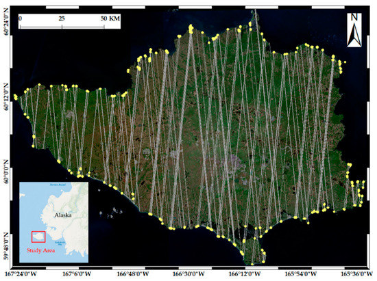
Figure 1.
Map of the Nunivak Island, which is near mainland Alaska. The background is a true-color image obtained using the Google Earth Engine and composed using the Sentinel-2 satellite during the summers of 2018 to 2020. The gray lines represent the ICESat-2 trajectory, and ICESat-2 passed through the region starting from 10/22/2018. The yellow areas represent shore zones, which contain ICESat-2 and multispectral data.
2.2. Materials
We used Sentinel-2 multispectral images and ICESat-2 data in the experiments. Launched by the European Space Agency (ESA), Sentinel-2 has 13 spectral bands with 10, 20, and 60 m ground resolutions, with a revisit period of 5 days [26]. Compared with the top of atmosphere reflectance data of level-1C, the level-2A data are preprocessed through radiometric calibration and atmospheric correction and directly represent the surface reflectance.
ICESat-2, launched by the National Aeronautics and Space Administration (NASA) in 2018, carries an ATLAS sensor that can acquire photon points of about 0.7 m in the along-track direction. ATLAS emits six laser beams arranged in three parallel groups; each group contains one strong and one weak signal, with an energy ratio of 4:1 [10,11]. The data are divided into three levels, with 21 standard data products stored in h5 hierarchical files. ICESat-2 Level-2 ATL03 geolocated photons are used in this paper, including raw photons (signal and noise photons); each photon has a unique latitude, longitude, and altitude based on the WGS84 ellipsoid benchmark [27].
We used ShoreZone data to verify our results. ShoreZone is a standardized coastal habitat mapping system that images and characterizes the biophysical attributes of discrete coastal units in a searchable, spatially explicit database, with the same standard protocols for acquiring, analyzing, and publishing coastal habitat information. For coastal zone areas, the ShoreZone classification is established by substrate (rock, gravel, sand, and different coastal substrate types), intertidal zone width, and slope [25]. Nunivak Island has a broad cross-section of coastal habitats, making it an ideal test area for the shore zone classification study.
3. Methods
3.1. Sentinel-2 Data Processing
Sentinel-2 image selection and processing should be performed before feature selection. The coastal zone is where land and water interface; it has a complex, dynamic environment affected by tides, sedimentation, and wave erosion [1,28]. Since the tidal action is long and periodic, the data obtained from satellites, such as multispectral or microwave radar, only reflect the situation of the coastal zone at the moment of transit and they are not universally available [28,29]. Additionally, errors caused by transient environmental factors, such as glint or cloud cover, can affect the quality of single multispectral image data and influence the final classification results. Therefore, we choose Google Earth Engine for data synthesis.
Google Earth Engine is a computing platform for global scale online processing analysis and visualization of geoscience datasets, especially remote sensing image data. The platform specializes in processing long time-series remote sensing data. It has been widely used in data fusion, multi-temporal image classification, change detection, land cover, and land use dynamics monitoring and modeling [20].
Nunivak Island is located at high latitude. There is no significant area of snow coverage in summer. Therefore, to align the data acquisition time with ICESat-2 as much as possible, we selected Sentinel-2 images for the summers of 2018 to 2020 for processing (1 June to 31 August of each year). Through operations such as de-clouding and median smoothing, the synthetic images to be used as the next classification step were obtained using the Google Earth Engine platform.
Next, we present the variables used as random forest classification characteristics. Spectra are important features in remote sensing images. We selected eight spectral bands of Sentinel-2 synthetic images as classification characteristics. Additionally, index features, such as normalized difference vegetation index (NDVI), normalized difference water index (NDWI), and normalized difference red edge index (NDRE), can contain richer content, more vivid ground attributes, and effectively improve the accuracy of feature classification. NDVI is a simple, effective, and empirical measure of surface vegetation conditions. It can be used to assess the vegetation distribution in the coastal zone region. NDWI is based on the principle of spectral difference between water bodies and terrestrial features in the red and infrared bands. NDRE calculated using the red-edge band of Sentinel-2 has obvious advantages for vegetation canopy chlorophyll detection. As such, it can be used to indicate the coastal zone environment. The specific information is shown in Table 1.

Table 1.
Sentinel-2 characteristic variables and description.
3.2. ICESat-2 Data Processing
The Geoscience Laser Altimeter System (GLAS) carried by ICESat is a full-waveform LiDAR. It responds to echo signals in a linear model and can detect the magnitude of echo signals. GLAS illuminates spots (footprints) 70 m in diameter, spaced at 170 m intervals along the Earth’s surface using laser pulses at 40 times per second [36]. The ATLAS on ICESat-2 is a new photon-counting LiDAR. It improves the detection efficiency significantly compared to GLAS, and its data do not contain the intensity of the echo signal and are more suitable for processing using statistical methods [10,11]. Based on the new characteristics of the ICESat-2 data, we selected a number of features that can be divided into two categories. First, statistical metrics are used: standard deviation (STD), relative standard deviation (Rstd), mean absolute deviation (MAD), quartile deviation (QD), relative average deviation (RAD), mean absolute error (MAE), median, and kurtosis and skewness. Second, the other indicators used are the coastal slope (Slope), signal-to-noise ratio (SNR), number of signal photons (Numbers), and the ratio of the number of photons between the upper and lower quartiles to the total number of photons (Ratio). The Slope is calculated from the upper and lower quartiles which reflects the morphological characteristics; the SNR represents the percentage of medium and high confidence photons. The specific information is shown in Table 2.
Table 2.
ICESat-2 characteristic variables and description.
In Table 2: hi is the elevation of each photon; h is the average elevation of photons; the third quartile (Q3) is the upper or 75th empirical quartile, as 75% of the data lies below this point; the first quartile (Q1) is the middle number between the smallest number (minimum) and median of the dataset; μ is the mean; and σ is the standard deviation. Therefore, to achieve high classification results, statistical indices related to the classification of coastal zone areas are calculated using medium and high confidence photons only, which are substituted into the calculation as characteristics for the random forest algorithms.
3.3. Sample Data Selection
Coastal zones reflect the interaction between land, atmosphere, and ocean, whose sediments and morphology contain information on sea-level change and coastal environmental evolution [1]. The concept of a shore zone is fundamental to delineating and classifying the mapping area. There are different ways to delineate the coastal zone. The narrow zone between high and low tides is delineated as a shore zone, which is obtained from elevation data and the astronomical tide. Additionally, coastal zones can be classified using bio bands or flood markers [22,37]. We chose the buffer method to delineate the coastal zone, given that the images used are synthetic, and the tides and seawater are smoothed out. In this paper, we define the coastal zone as a narrow area at a certain distance from the waterline to the landside in the image. The surface characteristics of the coastline splash zone on the high tide line are influenced by the shoreline type and can be considered as part of the characteristics of the shore type [37]. For this reason, the above distance is set to 100 m.
The quality of the samples directly affects the final classification results, and a representative and typical area should be selected as the sample. ICESat-2 makes passes over Nunivak Island 184 times. There are 1104 trajectories in the region as six beams are formed on the ground each time. In this study, photon trajectories with poor signal quality were excluded to ensure the accuracy of coastal feature extraction as much as possible (at least 50 photons). Finally, a total of 611 effective shore zones were selected. Several typical shore zone types are shown in Figure 2.
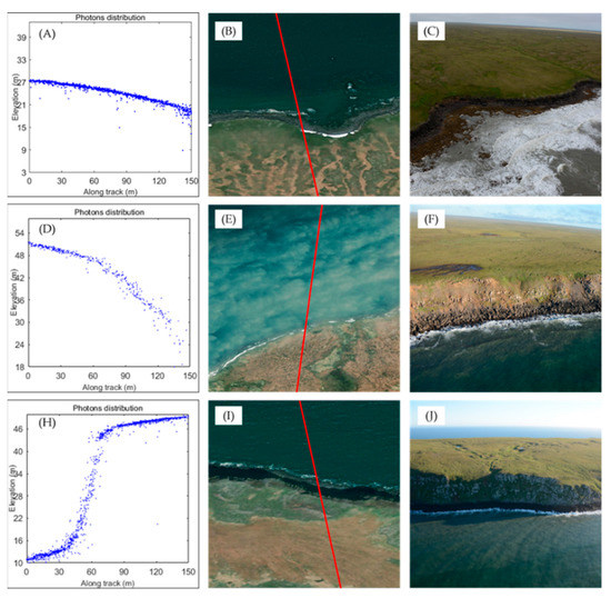
Figure 2.
The typical coastline of Nunivak Island. Different coastal zones are represented in a row: (1) (A–C) are the platform with a gravel beach, (2) (D–F) are ramps with a gravel beach, and (3) (H–J) are cliffs with a gravel beach. The left column is photons distribution from ICESat-2, and the middle column represents a true-color image. The right column corresponds to digital images from ShoreZone classification. The red line corresponds to the ICESat-2 track.
3.4. Random Forests and Feature Optimization
Random forest is an ensemble learning model based on decision tree classifiers. It is trained using the bagging method, and its final classification result is determined by the output vote of a single decision tree [18]. The steps of random forest establishment are as follows. First, training samples are selected from the original sample using the bootstrap method, which amounted to about 63% of the overall samples. Additionally, decision trees are built based on the training samples to form a random forest. In the training process, features are randomly selected at each tree node (usually less than the total number of features). Then, a feature with the most classification ability is selected for node splitting inside the decision tree according to the principle of minimum Gini coefficient or entropy. Finally, the random forest classifier formed by multiple decision trees can classify the data and decide the class by decision trees’ voting. In this process, the selection of training samples and feature subsets is random and independent. The philosophy behind random forest algorithms is based on the basic premise that a set of classifiers performs better classifications than a single classifier [18]. Random forests present many advantages, such as providing estimates of what variables are important in the classification, being robust to outliers, and noise [38]. The random forest algorithm estimates the importance of variables based on the principle that randomly rearranging the order of the features to be evaluated affects a change in prediction error. The importance of a variable can be derived from the predicted value and standard deviation [17,18].
In this paper, we randomly selected 80% of the total samples for training and designed four protocols for comparative study (Table 3). The two main purposes for setting different solutions are as follows. The first is to investigate the influence of different variables on the accuracy of shore zone classification and determine the variable importance. The second is to explore the best method for coastal zone classification through comparison.
Table 3.
Information of experimental protocols.
4. Results
In this section, we demonstrate the variable importance and classification results using the methods and data described above.
4.1. Importance of Variables
We obtained the importance of each feature variable using the random forest algorithm. Figure 3 shows the results in detail. As shown in the figure, band 4 (red band), band 12 (SWIR 2 band), band 2 (blue band), and band 3 (green band) are more important than others in the Sentinel-2 features, which are all key spectral variables. Additionally, index features, such as NDVI and NDWI, are of high importance. For the variables obtained from ICESat-2 data, the Slope, STD, and median variables are of high importance, and these features can adequately characterize the shoreline morphology. Generally, the Sentinel-2 features are more important than the ICESat-2 features. This means that multispectral satellites can obtain richer surface information, important data for land use, and coastal zone classification. Meanwhile, the addition of ICESat-2 data can improve classification accuracy.
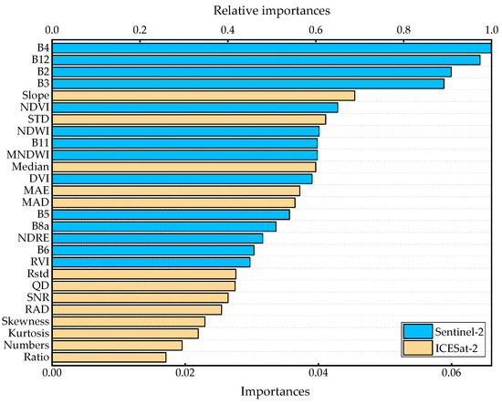
Figure 3.
Distribution of characteristic importance. The feature importance is normalized to highlight the percentage of each variable. The blue column is the characteristic variable of Sentinel-2, whereas the yellow column corresponds to ICESat-2.
We rearranged the features according to variable importance. Then, we added them sequentially to the random forest model for training to observe the changes in classification accuracy and the kappa coefficient to find the optimal combination model. Figure 4 shows that the classification accuracy increases sharply from 34.14% to 76.29% as the features increase from 2 to 9. The accuracy rises slowly when the number of variables is between 9 and 21 and reaches the highest classification accuracy of 83.61% at 21. The accuracy gradually decreases when the number of features exceeds 21. Similarly, the kappa coefficient reaches the highest value of 0.81 when the number of features is 21. Therefore, the number of features was set to 21, which achieves relatively higher accuracy whilst simultaneously reducing the calculation amount.
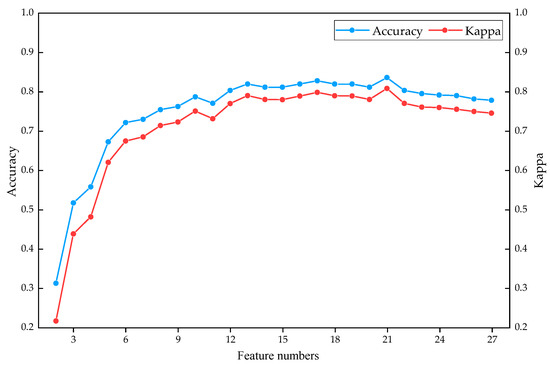
Figure 4.
Relationship between the number of characteristic variables and classification accuracy and the kappa coefficient. The blue line represents the classification accuracy, whereas the red line corresponds to the kappa coefficient.
Table 4 presents the classification accuracies and kappa coefficients for each experimental scheme. As presented in the table, for the shoreline classification results obtained using the four methods, the kappa coefficients ranged from 0.31 to 0.81, with an average of 0.63. The overall classification accuracies ranged from 42.63% to 83.61%, with an average of 68.02%. The feature parameters obtained from Sentinel-2 prediction results are better than ICESat-2, and the optimal solution has better performance in terms of classification accuracy and consistency.
Table 4.
Results of experimental protocols.
4.2. Classification Results of Shore Zone
Next, using the trained random forest model and the preferred feature parameters, the classification results for the coastline of Nunivak Island were generated (Figure 5 and Figure 6). Figure 5 demonstrates the classification results for the whole of Nunivak Island, and Figure 6 shows details for the southeastern part of the island. We can evaluate the performance of each model by comparing the predicted results with the in situ data.
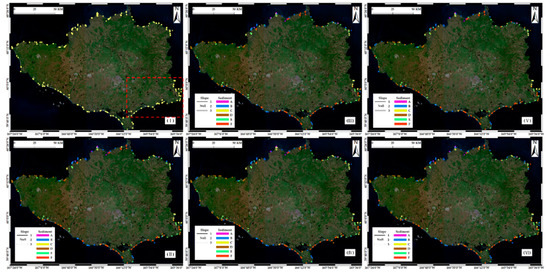
Figure 5.
Shore zone type results for Nunivak Island using different methods. (I) Sentinel-2 imagery of Nunivak Island before classification; (II) shore zone types from the ShoreZone classification; (III–VI) coastline classification results derived from the optimal features, all features, Sentinel-2 features, and ICESat-2 features, respectively. The colors represent the coastal types according to sediment and substrate: (A) rock, (B) rock & gravel, (C) rock & gravel & sand, (D) gravel, (E) sand & gravel, and (F) sand & mud. The line shapes represent the type of shore zone by slope: (1) flat, (2) inclined, and (3) steep. The red box corresponds to the area (to illustrate the detailed classification results) in Figure 6.
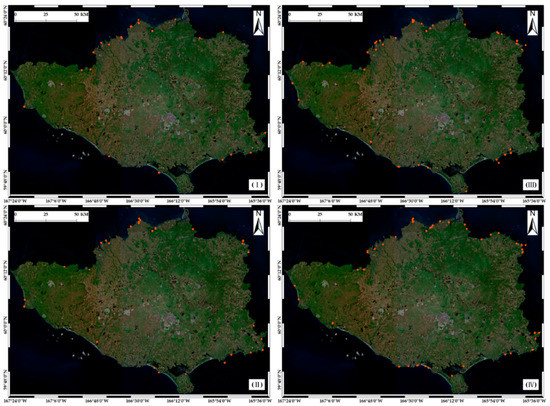
Figure 6.
Detailed results of the coastal zone classification by comparison with the validation data. (I–IV) Coastline classification error results derived from the optimal features, all features, Sentinel-2 features, and ICESat-2 features, respectively. We only show the misclassification results in Figure 6, which are indicated in red colors.
The coastal zone area of the island is relatively developed and has a wide variety of coastal zone types. Therefore, to present the classification results in a more reasonable way, we distinguished the shoreline types according to the coastal morphology (flat, inclined, and steep) and substrate sediments (rock, rock & gravel, rock & gravel & sand, gravel, sand & gravel, and sand & mud). This is consistent with the classification principles of the validation dataset ShoreZone classification, which we used to validate the prediction results (Appendix A, Table A1).
In terms of coastal morphology, the coasts of Nunivak Island are mostly flat and inclined. Steep coasts are relatively rare and distributed mostly in the western and northern parts of the island. Figure 6 reveals detailed results of the coastal zone classification by comparing it with the validation data. The optimal combination model performed better in the morphological classification of the coast compared with other schemes.
5. Discussions
5.1. Misclassification Analysis
Our method classifies shore type from the sedimentary and morphological parameters with an overall accuracy of 83.61% on the test datasets. Table 5 presents the confusion matrix of the model prediction results based on ShoreZone datasets. The producer’s and user’s accuracies of the model prediction results are satisfactory; however, there are still misclassification cases. Based on the confusion matrix, we analyze the reasons for the misclassification as follows.
Table 5.
Confusion matrix of test samples using optimal features predicted, overall accuracy: 83.61%.
First, there are more commission errors in the sample of category 9 (ramp with gravel beach) and more omission errors in the sample of category 7 (platform with gravel beach, wide); they are both sedimentary beaches with gravel morphology [25]. Nunivak Island has long gravel beaches with well-developed coastal zones around the island; gravel beaches have high intra-class variability and are easily confused with other similar beach categories [25]. With manual discrimination, gravel beaches can be difficult to distinguish accurately from gravelly semi-depositional beaches. Furthermore, our study area is delineated based on the shore-water interface line, which is different from the coastal zone classification of the reference data. In the current ShoreZone classification systems, the extent of the coastal zone is usually derived from visible clues, such as tide marks and water level at the time of the photo collection [22]. In this paper, the multispectral data were synthesized using the Google Earth Engine. Although this effectively suppresses the chance of error, smoothed out tidal signs result in the tides in the synthesized images being only the adjusted mean values. We applied a buffer zone approach to determine the extent of the study area. This is because the intertidal delineation using tidal features is impossible on synthetic imagery. This approach differs from the traditional way of describing the coastal zone, which affects the accuracy of coastal zone feature extraction. Additionally, tides, wind, and waves can affect the ICESat-2 satellite measurements. The potential reasons for this are as follows. In the flat and shallow coastline, high confidence photons are obtained from the sea surface and seafloor. Due to the shallow water depth, the photon signals are mixed, and the signal types cannot be effectively distinguished to extract the underwater shoreline. On the steep and deep coast, rising tides can mask the shore morphology, resulting in photons acquiring only surface information [9,39,40].
5.2. Analysis of Important Variables
We used a random forest algorithm to obtain the variable importance for shore zone classification, using the Sentinel-2 and ICESat-2 variables. First, the most important variables derived from Sentinel-2 are band values (B4, B12, B2, and B3) and NDVI. Visible and short-wave infrared bands are good for detecting coastal zone areas. The visible band is susceptible to thin clouds in a single image, leading to limited usability; however, this problem does not seem to exist in synthetic images [41]. NDVI facilitates the detection of terrestrial vegetation, which marks a transition from ocean processes to terrestrial processes, and vegetation can provide a natural and process-based shore zone boundary [8]. Second, the statistical features calculated from the medium and high confidence photons are related to shore zone type, and their importance can be assessed using the random forest model. The important variables, other than those derived from Sentinel-2, consist of the Slope, STD, median, MAE, and MAD. Statistical feature information derived from airborne LiDAR and ICESat-2 are good predictors of coastal area [21]. Xie et al. [23] used ICESat-2 metrics and a SoftMax regression model for shore zone classification. Nijland et al. [22] estimated coastal information on Calvert Island using LiDAR data and compared it to the ShoreZone classification. Third, and overall, most of the important variables are obtained from multispectral data. This emphasizes the efficacy of Sentinel-2 data in coastal zone classification. Although precise elevation information cannot be obtained as with ICESat-2, Sentinel-2 data have multiband spectral information and can reveal environmental changes.
5.3. Contributions of ICESat-2
ICESat-2 is an ideal data source for detailed coastal zone morphological metrics. The contributions and advantages of the ICESat-2 on the shore zone study are as follows. (1) ATLAS features the ability to acquire land–water interaction zone information because of its improved along-track sampling interval (0.7 m) and blue–green laser pulses (532 mm) [10,11]. Traditional LiDAR data applied terrestrially often have a limited spatial application on the marine side of the coastal zone. Due to its inability to penetrate the water column, the information obtained is limited to tide elevations at the time of data acquisition [22,42]. ICESat-2 and airborne LiDAR bathymetry (ALB) make it suitable for detecting shallow water bathymetry, expanding the elevation data beyond the sea surface, where traditional methods do not provide data. (2) ICESat-2 has the advantage of higher resolution, rich terrain information, and is an ideal method for monitoring change in the coastal environments. Elevation data provide important information about shore metrics and coastline position; it can be used for analysis or change detection purposes [37]. The elevation-based morphological data can be used to predict vegetation patterns, soil properties, and mapping of habitat types on the seabed, which can reduce coordinate system conversion errors compared with those of traditional land–water separation measurements [22,37]. (3) LiDAR can provide vertical forest structure information that can be effectively used for forest height and biomass estimation in coastal zone areas, which are difficult to reach using traditional measurement methods. Additionally, ICESat-2, the satellite photon-counting LiDAR, can be followed for mapping and monitoring forest biomass or carbon stock at local to global levels, if it became necessary to consider the seasonal behavior of deciduous forests [8,43].
5.4. Superiority, Limitations, and Suggestions
The superiority of the method presented in this paper is as follows. (1) The study explored the potential to include information obtained from satellite data directly into the coastal classification. ICESat-2 and Sentinel-2 data are freely available. Therefore, this method is cost-effective, reducing the need for manual photo interpretations. (2) The proposed method, combined with multispectral and ICESat-2 data, can be applied to shore zone and areas around islands; it is also essential for hard-to-reach inland waters, such as plateau lakes [44]. Utilizing free satellite data, we can quickly and efficiently obtain detailed information about water–land interface regions on a global scale.
The proposed method has a few limitations. First, the method is less precise than classification results that rely heavily on oblique photography and expert interpretation. For applications that need accurate information on the coastal zone, the proposed method should be used with caution. Second, in our method, the delineation of the shore boundaries cannot be defined by visual cues due to the use of synthetic images, leading to a poor delineation of the shore zone.
In this study, the innovation attempted was the incorporation of ICESat-2 derived morphological metrics into the spectral variables of shore zone classification. Additionally, the ICESat-2 data do not provide a wall-to-wall spatial coverage [27]. Integrating ICESat-2, multispectral, and SAR with other forms of data, and using machine learning algorithms to monitor and classify the shore area, may have significant potential in the future.
6. Conclusions
This paper proposed a classification coastline method using random forest algorithms based on multispectral and ICESat-2 data remote sensing. First, remote sensing images of Sentinel-2 data for Nunivak Island in the summer were composed using Google Earth Engine, a method that can effectively suppress the chance of errors. We calculated data features based on the integrated multispectral data. Second, statistical indicators related to the slope and sediment classification were extracted based on ICESat-2 high confidence photons. Third, the characteristics extracted from the multispectral image and ICESat-2 were used to train the random forest model separately. The results were compared with the optimized features. The experimental results show that the overall accuracy and kappa coefficient for optimizing features is 83.61% and 0.81, respectively, which were superior to others. Additionally, the variable importance was analyzed. The misclassification cases were also carefully analyzed, and the reasons were summarized. In future studies, ICESat-2 can provide various accurate along-track photons when used alongside the multispectral satellite. Using this method, accurate coastline information can be obtained for coastal areas, the area surrounding islands, and reefs, on a global scale, especially in remote and sensitive areas.
Author Contributions
Conceptualization, C.L.; methodology, C.L.; software, C.L.; validation, C.L. and J.Q.; formal analysis, J.Q.; investigation, C.L.; data curation, C.L. and J.Q.; writing—original draft preparation, C.L. and Q.T.; writing—review and editing, J.L., and X.Z.; visualization, J.Q.; supervision, J.L. and Q.T.; project administration, J.L. and Q.T.; funding acquisition, J.L. and Q.T. All authors have read and agreed to the published version of the manuscript.
Funding
This research is funded by the National Natural Science Foundation of China (41876111, 41871381); Key Laboratory of Ocean Geomatics, Ministry of Natural Resources, China (Grant No.2021B04); and Chinese Arctic and Antarctic Administration Project (IRASCC 2020-2022).
Acknowledgments
We thank the NASA NSIDC for distributing the ICESat-2 data; the European Space Agency (ESA) for distributing the Sentinel-2 imagery. Furthermore, we thank the anonymous reviewers and members of the editorial team for their constructive comments.
Conflicts of Interest
The authors declare that they have no known competing financial interests or personal relationships that could influence the work reported in this paper.
Appendix A
Table A1.
Summary of shore zone types.
Table A1.
Summary of shore zone types.
| Substrate | Sediment | With | Slope | Coastal Class |
|---|---|---|---|---|
| Rock | n/a | Wide (>30 m) | Steep (>20 degree) | n/a |
| Inclined (5–20 degree) | Rock Ramp, wide (1) | |||
| Flat (<5 degree) | Rock Platform, wide (2) | |||
| Narrow (<30 m) | Steep (>20 degree) | Rock Cliff (3) | ||
| Inclined (5–20 degree) | Rock Ramp, narrow (4) | |||
| Flat (<5 degree) | Rock Platform, narrow (5) | |||
| Rock & Sediment | Gravel | Wide (>30 m) | Steep (>20 degree) | n/a |
| Inclined (5–20 degree) | Ramp with gravel beach, wide (6) | |||
| Flat (<5 degree) | Platform with gravel beach, wide (7) | |||
| Narrow (<30 m) | Steep (>20 degree) | Cliff with gravel beach (8) | ||
| Inclined (5–20 degree) | Ramp with gravel beach (9) | |||
| Flat (<5 degree) | Platform with gravel beach (10) | |||
| Gravel & Sand | Wide (>30 m) | Steep (>20 degree) | n/a | |
| Inclined (5–20 degree) | Ramp with gravel/sand beach, wide (11) | |||
| Flat (<5 degree) | Platform with gravel/sand beach, wide (12) | |||
| Narrow (<30 m) | Steep (>20 degree) | Cliff with gravel/sand beach (13) | ||
| Inclined (5–20 degree) | Ramp with gravel/sand beach (14) | |||
| Flat (<5 degree) | Platform with gravel/sand beach (15) | |||
| Sand | Wide (>30 m) | Steep (>20 degree) | n/a | |
| Inclined (5–20 degree) | Ramp with sand beach, wide (16) | |||
| Flat (<5 degree) | Platform with sand beach, wide (17) | |||
| Narrow (<30 m) | Steep (>20 degree) | Cliff with sand beach (18) | ||
| Inclined (5–20 degree) | Ramp with sand beach (19) | |||
| Flat (<5 degree) | Platform with sand beach (20) | |||
| Sediment | Gravel | Wide (>30 m) | Flat (<20 degree) | Gravel flat, wide (21) |
| Narrow (<30 m) | Steep (>20 degree) | n/a | ||
| Inclined (5–20 degree) | Gravel beach, narrow (22) | |||
| Flat (<5 degree) | Gravel flat or fan (23) | |||
| Gravel & Sand | Wide (>30 m) | Steep (>20 degree) | n/a | |
| Inclined (5–20 degree) | n/a | |||
| Flat (<5 degree) | Sand/Gravel flat or fan (24) | |||
| Narrow (<30 m) | Steep (>20 degree) | n/a | ||
| Inclined (5–20 degree) | Sand/Gravel beach, narrow (25) | |||
| Flat (<5 degree) | Sand/Gravel flat or fan (26) | |||
| Sand & Mud | Wide (>30 m) | Steep (>20 degree) | n/a | |
| Inclined (5–20 degree) | Sand beach (27) | |||
| Flat (<5 degree) | Sand flat (28) | |||
| Flat (<5 degree) | Mudflat (29) | |||
| Narrow (<30 m) | Steep (>20 degree) | n/a | ||
| Inclined (5–20 degree) | Sand beach (30) | |||
| Flat (<5 degree) | n/a |
References
- Nicholls, R.J.; Cazenave, A. Sea-level rise and its impact on coastal zones. Science 2010, 328, 1517–1520. [Google Scholar] [CrossRef] [PubMed]
- Murray, N.J.; Phinn, S.R.; DeWitt, M.; Ferrari, R.; Johnston, R.; Lyons, M.B.; Clinton, N.; Thau, D.; Fuller, R.A. The global distribution and trajectory of tidal flats. Nature 2019, 565, 222–225. [Google Scholar] [CrossRef] [PubMed]
- Gon, C.C.; Alves, G.; Santos, S.; Duarte, D.; Gomes, J.E. Monitoring Local Shoreline Changes by Integrating UASs, Airborne LiDAR, Historical Images and Orthophotos. GISTAM 2019, 126–134. [Google Scholar] [CrossRef]
- Xu, W.; Guo, K.; Liu, Y.; Tian, Z.; Tang, Q.; Dong, Z.; Li, J. Refraction error correction of Airborne LiDAR Bathymetry data considering sea surface waves. Int. J. Appl. Earth Obs. 2021, 102, 102402. [Google Scholar] [CrossRef]
- Bishop-Taylor, R.; Nanson, R.; Sagar, S.; Lymburner, L. Mapping Australia’s dynamic coastline at mean sea level using three decades of Landsat imagery. Remote Sens. Environ. 2021, 267, 112734. [Google Scholar] [CrossRef]
- Poursanidis, D.; Traganos, D.; Reinartz, P.; Chrysoulakis, N. On the use of Sentinel-2 for coastal habitat mapping and satellite-derived bathymetry estimation using downscaled coastal aerosol band. Int. J. Appl. Earth Obs. 2019, 80, 58–70. [Google Scholar] [CrossRef]
- Mishra, M.K.; Ganguly, D.; Chauhan, P.; Ajai. Estimation of coastal bathymetry using RISAT-1 C-band microwave SAR data. IEEE Geosci. Remote Sens. Lett. 2014, 11, 671–675. [Google Scholar] [CrossRef]
- Nandy, S.; Srinet, R.; Padalia, H. Mapping Forest Height and Aboveground Biomass by Integrating ICESat-2, Sentinel-1 and Sentinel-2 Data Using Random Forest Algorithm in Northwest Himalayan Foothills of India. Geophys. Res. Lett. 2021, 48, e2021GL093799. [Google Scholar] [CrossRef]
- Ma, Y.; Xu, N.; Liu, Z.; Yang, B.; Yang, F.; Wang, X.H.; Li, S. Satellite-derived bathymetry using the ICESat-2 lidar and Sentinel-2 imagery datasets. Remote Sens. Environ. 2020, 250, 112047. [Google Scholar] [CrossRef]
- Markus, T.; Neumann, T.; Martino, A.; Abdalati, W.; Brunt, K.; Csatho, B.; Farrell, S.; Fricker, H.; Gardner, A.; Harding, D.; et al. The Ice, Cloud, and land Elevation Satellite-2 (ICESat-2): Science requirements, concept, and implementation. Remote Sens. Environ. 2017, 190, 260–273. [Google Scholar] [CrossRef]
- Neumann, T.A.; Martino, A.J.; Markus, T.; Bae, S.; Bock, M.R.; Brenner, A.C.; Brunt, K.M.; Cavanaugh, J.; Fernandes, S.T.; Hancock, D.W.; et al. The Ice, Cloud, and Land Elevation Satellite—2 mission: A global geolocated photon product derived from the Advanced Topographic Laser Altimeter System. Remote Sens. Environ. 2019, 233, 111325. [Google Scholar] [CrossRef] [PubMed]
- Mas, J.F.; Flores, J.J. The application of artificial neural networks to the analysis of remotely sensed data. Int. J. Remote Sens. 2008, 29, 617–663. [Google Scholar] [CrossRef]
- Quinlan, J.R. Induction of Decision Trees. Mach. Learn. 1986, 1, 81–106. [Google Scholar] [CrossRef] [Green Version]
- Cortes, C.A.V.V. Support Vector Networks. Mach. Learn. 1995, 20, 273–297. [Google Scholar] [CrossRef]
- Breiman, L. Bagging Predictors. Mach. Learn. 1996, 24, 123–140. [Google Scholar] [CrossRef] [Green Version]
- Freund, Y.; Schapire, R.E. A Decision-Theoretic Generalization of On-Line Learning and an Application to Boosting. J. Comput. Syst. Sci. 1997, 55, 119–139. [Google Scholar] [CrossRef] [Green Version]
- Bühlmann, P. Bagging, Boosting and Ensemble Methods. In Handbook of Computational Statistics, Gentle, J., Härdle, W., Mori, Y.; Springer: Berlin, Germany, 2012. [Google Scholar]
- Breiman, L. Random Forests. Mach. Learn. 2001, 45, 5–32. [Google Scholar] [CrossRef] [Green Version]
- Rodriguez-Galiano, V.F.; Ghimire, B.; Rogan, J.; Chica-Olmo, M.; Rigol-Sanchez, J.P. An assessment of the effectiveness of a random forest classifier for land-cover classification. ISPRS J. Photogramm. 2012, 67, 93–104. [Google Scholar] [CrossRef]
- Gorelick, N.; Hancher, M.; Dixon, M.; Ilyushchenko, S.; Thau, D.; Moore, R. Google Earth Engine: Planetary-scale geospatial analysis for everyone. Remote Sens. Environ. 2017, 202, 18–27. [Google Scholar] [CrossRef]
- Manzo, C.; Valentini, E.; Taramelli, A.; Filipponi, F.; Disperati, L. Spectral characterization of coastal sediments using Field Spectral Libraries, Airborne Hyperspectral Images and Topographic LiDAR Data (FHyL). Int. J. Appl. Earth Obs. 2015, 36, 54–68. [Google Scholar] [CrossRef]
- Nijland, W.; Reshitnyk, L.Y.; Starzomski, B.M.; Reynolds, J.D.; Darimont, C.T.; Nelson, T.A. Deriving Rich Coastal Morphology and Shore Zone Classification from LIDAR Terrain Models. J. Coastal Res. 2017, 33, 949–958. [Google Scholar] [CrossRef]
- Xie, H.; Sun, Y.; Liu, X.; Xu, Q.; Guo, Y.; Liu, S.; Xu, X.; Liu, S.; Tong, X. Shore Zone Classification from ICESat-2 Data over Saint Lawrence Island. Mar. Geod. 2021, 454–466. [Google Scholar] [CrossRef]
- Feng, Q.; Liu, J.; Gong, J. UAV Remote Sensing for Urban Vegetation Mapping Using Random Forest and Texture Analysis. Remote Sens. 2015, 7, 1074–1094. [Google Scholar] [CrossRef] [Green Version]
- Harper, J.R.; Morris, M.C. Alaska ShoreZone Coastal Habitat Mapping Protocol. Prepared for Bureau of Ocean Energy Management (BOEM), Anchorage, AK. Prepared by Nuka Research and Planning Group LLC, Soldovia, AK. 2014; 164p. Available online: http://alaskafisheries.noaa.gov/shorezone/chmprotocol0114.pdf (accessed on 12 October 2021).
- Drusch, M.; Del Bello, U.; Carlier, S.; Colin, O.; Fernandez, V.; Gascon, F.; Hoersch, B.; Isola, C.; Laberinti, P.; Martimort, P.; et al. Sentinel-2: ESA’s Optical High-Resolution Mission for GMES Operational Services. Remote Sens. Environ. 2012, 120, 25–36. [Google Scholar] [CrossRef]
- Neumann, T.; Brenner, A.; Hancock, D.; Robbins, J.; Saba, J.; Harbeck, K.; Gibbons, A. Ice, Cloud, and Land Elevation Satellite--2 (ICESat-2) Project: Algorithm Theoretical Basis Document (ATBD) for Global Geolocated Photons (ATL03); National Aeronautics and Space Administration, Goddard Space Flight Center: Greenbelt, MD, USA, 2019.
- Randazzo, G.; Cascio, M.; Fontana, M.; Gregorio, F.; Lanza, S.; Muzirafuti, A. Mapping of Sicilian Pocket Beaches Land Use/Land Cover with Sentinel-2 Imagery: A Case Study of Messina Province. Land 2021, 10, 678. [Google Scholar] [CrossRef]
- Arjasakusuma, S.; Kusuma, S.S.; Saringatin, S.; Wicaksono, P.; Mutaqin, B.W.; Rafif, R. Shoreline Dynamics in East Java Province, Indonesia, from 2000 to 2019 Using Multi-Sensor Remote Sensing Data. Land 2021, 10, 100. [Google Scholar] [CrossRef]
- Tucker, C.J. Red and photographic infrared linear combinations for monitoring vegetation. Remote Sens. Environ. 1979, 8, 127–150. [Google Scholar] [CrossRef] [Green Version]
- Rouse, J.W.; Haas, R.U.D.H.; Schell, J.A.; Deering, D.W. Monitoring Vegetation Systems in the Great Plains with ERTS; NASA Special Publication: Washington, DC, USA, 1974; Volume 351, p. 309.
- Gao, B. NDWI—A normalized difference water index for remote sensing of vegetation liquid water from space. Remote Sens. Environ. 1996, 58, 257–266. [Google Scholar] [CrossRef]
- Han-Qiu, X.U. A study on information extraction of water body with the modified normalized difference water index (MNDWI). J. Remote Sens. 2005, 5, 589–595. [Google Scholar]
- Thompson, C.N.; Guo, W.; Sharma, B.; Ritchie, G.L. Using normalized difference red edge index to assess maturity in cotton. Crop Sci. 2019, 59, 2167–2177. [Google Scholar] [CrossRef]
- Major, D.J.; Baret, F.E.D.E.; Guyot, G. A ratio vegetation index adjusted for soil brightness. Int. J. Remote Sens. 1990, 11, 727–740. [Google Scholar] [CrossRef]
- Abshire, J.B.; Sun, X.; Riris, H.; Sirota, J.M.; McGarry, J.F.; Palm, S.; Yi, D.; Liiva, P. Geoscience laser altimeter system (GLAS) on the ICESat mission: On-orbit measurement performance. Geophys. Res. Lett. 2005, 32. [Google Scholar] [CrossRef] [Green Version]
- Mason, D.C.; Gurney, C.; Kennett, M. Beach topography mapping—a comparsion of techniques. J. Coast. Conserv. 2000, 6, 113–124. [Google Scholar] [CrossRef]
- Zi--chen, G.; Tao, W.; Shu--lin, L.; Wen--ping, K.; Xiang, C.; Kun, F.; Ying, Z. Comparison of the backpropagation network and the random forest algorithm based on sampling distribution effects consideration for estimating nonphotosynthetic vegetation cover. Int. J. Appl. Earth Obs. 2021, 104, 102573. [Google Scholar] [CrossRef]
- Parrish, C.E.; Magruder, L.A.; Neuenschwander, A.L.; Forfinski-Sarkozi, N.; Alonzo, M.; Jasinski, M. Validation of ICESat-2 ATLAS Bathymetry and Analysis of ATLAS’s Bathymetric Mapping Performance. Remote Sens. 2019, 11, 1634. [Google Scholar] [CrossRef] [Green Version]
- Liu, C.; Qi, J.; Li, J.; Tang, Q.; Xu, W.; Zhou, X.; Meng, W. Accurate Refraction Correction—Assisted Bathymetric Inversion Using ICESat-2 and Multispectral Data. Remote Sens. 2021, 13, 4355. [Google Scholar] [CrossRef]
- Zhao, Y.; An, R.; Xiong, N.; Ou, D.; Jiang, C. Spatio-Temporal Land-Use/Land-Cover Change Dynamics in Coastal Plains in Hangzhou Bay Area, China from 2009 to 2020 Using Google Earth Engine. Land 2021, 10, 1149. [Google Scholar] [CrossRef]
- Mohamed, M.A. Classification of Landforms for Digital Soil Mapping in Urban Areas Using LiDAR Data Derived Terrain Attributes: A Case Study from Berlin, Germany. Land 2020, 9, 319. [Google Scholar] [CrossRef]
- Zhang, J.; Tian, J.; Li, X.; Wang, L.; Chen, B.; Gong, H.; Ni, R.; Zhou, B.; Yang, C. Leaf area index retrieval with ICESat-2 photon counting LiDAR. Int. J. Appl. Earth Obs. 2021, 103, 102488. [Google Scholar] [CrossRef]
- Cooley, S.W.; Ryan, J.C.; Smith, L.C. Human alteration of global surface water storage variability. Nature 2021, 591, 78–81. [Google Scholar] [CrossRef]
Publisher’s Note: MDPI stays neutral with regard to jurisdictional claims in published maps and institutional affiliations. |
© 2022 by the authors. Licensee MDPI, Basel, Switzerland. This article is an open access article distributed under the terms and conditions of the Creative Commons Attribution (CC BY) license (https://creativecommons.org/licenses/by/4.0/).