Abstract
Although many prior studies have found that landscape pattern significantly affects urban heat environment globally, the spatially heterogeneous in the cooling effects of landscape pattern remains poorly understood. In addition, most previous studies have only employed a single landscape metric separately, without holistic consideration of the composition and configuration of different landscapes. Taking one of the new “stove” cities in China-Fuzhou City, Fujian Province, as an example, we employed the principal component analysis (PCA) to synthesize a landscape pattern comprehensive index (LPCI) composed of the four common landscape metrics (i.e., aggregation index, AI; mean patch area, Area mn; largest patch index, LPI; and percentage of landscape, PLAND) of the three major land surfaces (i.e., water, vegetation, and impervious surface). Then, the local model (geographically weighted regression, GWR) was proposed to explore the spatially heterogeneous in the cooling effects of urban landscape. The results revealed that: (1) from 2000 to 2016, the land surface temperature (LST) increased by 4.262 °C, and the proportion of the urban heat island region showed an upward trend, while the urban-heat-island ratio index (URI) increased from 0.328 to 0.457; (2) the cooling effect of different land surfaces ranked from high to low was: water (29.69 °C), vegetation (38.56 °C), and impervious surface (41.82 °C); (3) compared with vegetation patches, water patches had a more obvious cooling effect on the surrounding environment, with the cooling distance within 60–90 m for the vegetation, while reaching 120–150 m for water body; (4) the proposed LPCI could explain more than 80% of the information for all of the landscape metrics for all of the landscape types, and presented a patchy distribution in the study area; (5) the GWR results revealed that the cooling effect of the landscape pattern varied spatially across the study area, indicating that the configuration of landscapes is more important in an urban center in alleviating urban heat environment than in an urban fringe area. The proposed approach provides a new understanding of the interaction between the landscape patterns and urban heat environments, providing a strong basis for landscape planning strategies for specific local sites.
1. Introduction
China’s urbanization rate had reached 60.60% by 2019 [1]. Urbanization changes the structure of a city’s underlying surface [2], combining with the heat emission from human activities, which lead to the phenomenon of concern, that is the well-known urban heat island effects (UHI) [3,4]. The UHI was defined as the surface temperature of urban areas and is significantly higher than that of suburban areas [5]. That is the result of the continuous reduction of vegetation due to the increasing number of impervious surfaces with huge heat storage capacity. Moreover, the tremendous heat generated by urban motor vehicles and human activities also exacerbates such phenomena. The UHI can aggravate air pollution [6], result in extremely bad weather conditions (e.g., strong winds and storms), and seriously affect both the physical and mental health of people [7,8,9], and thus the quality of life of urban residents [5,10,11]. Therefore, the cooling effects of landscape on the UHI have become a global research hotspot [12,13,14] to explore technologies and strategies for urban planners to alleviate urban thermal environment.
Fujian province is located on the southeast coast of China. It has a warm and humid climate and its terrain is mainly mountainous and hills. Its forest coverage rate has ranked first in China for 40 consecutive years. As the capital city of Fujian province, Fuzhou is famous for its reputation of being the “National Forest City” and “China’s Climate Eco-City”. Since China’s reformation and opening up, Fuzhou has implemented the strategy of “moving east and expanding south”, and its main urban area has continually been expanding. By the end of 2018, the urbanization rate of Fuzhou exceeded 70%. With the continuous acceleration of urbanization and the expansion of built-up areas, the urban landscape pattern of Fuzhou has undergone significant changes, and the impervious surface area has increased significantly, while the area of vegetation and water has decreased dramatically [11]. In addition, the basin terrain and high-rise buildings have blocked the main air ducts of the city, leading to the LST rising faster in urban areas than rural areas, and an increased UHI effect as a consequence. Recently, Fuzhou became the top of China’s new “furnaces” [11]. Therefore, it is of the utmost urgency that the optimization of landscape pattern to maximize its ability to mitigate the UHI is explored.
The purposes of this study are to: (1) observe the spatio-temporal evolution of the UHI in the urban area; (2) compare the cooling effect of water patches and vegetation patches; (3) investigate the spatially heterogeneous in the cooling effects of the integrated urban landscape pattern and identify its relative contributions to the urban heat environment. Based on these purposes, in this study we initially used the principal component analysis (PCA) method to synthesize a landscape pattern comprehensive index (LPCI) composed of the four common landscape metrics (i.e., aggregation index, AI; mean patch area, Area_mn; largest patch index, LPI; and percentage of landscape, PLAND) of the three major land surfaces (i.e., water, vegetation, and impervious surface). Then, unlike previous studies that only treat the UHI mechanism at a global level, we further employed the geographically weighted regression (GWR) to explore the spatially heterogeneous in the cooling effects of urban landscape. The proposed approach can provide a new understanding of the interactions between landscape patterns and urban heat environments.
2. Research Review
The land surface temperature (LST) is an important index to analyze and study UHI [14]. To monitor the LST in a wide range in real time, it is convenient to use thermal infrared remote sensing technology [6,15,16]. A variety of LST retrieval algorithms have been proposed, such as generalized single-channel algorithm, split-window algorithm, and radiation transfer equation method, etc. [17,18,19,20]. The research has shown that the retrieval accuracy ranges from high to low as: split-window algorithm > generalized single-channel algorithm > radiation transfer equation method [16,18]. In China, many studies have employed LST to explore the spatio-temporal evolution characteristics of the UHI for megacities, such as Beijing, Shanghai, and Xi’an, respectively [21,22,23]. Recently, the urban-heat-island ratio index (URI) was coined [24] and frequently used to evaluate the UHI, and to observe the evolution of the heat island [11,25,26]. For example, Liu et al. [6] estimated, respectively, the heat island intensity and its range in Beijing at different periods using the quantitative URI, and evaluated the status of UHI condition of Beijing plain regions, indicating that the UHI effect in Beijing continued to increase from 1987 to 2001. The URI is a quantitative index that overcomes the influence of temporal and spatial differences, which can effectively evaluate the intensity of UHI in different time phases and different regions [4,27].
The spatio-temporal distribution of LST is closely related to climatic conditions, the extent and the nature of underlying surface, population density, and other factors [28,29]. Of these, the land surface parameters (e.g., impervious surface, vegetation, water) have some of the greatest impacts on the urban thermal environment [3,30]. In terms of urban green space, some researchers explored the differences in cooling effects of different types of urban green land [31,32]. The normalized difference vegetation index (NDVI) was also extensively used to represent greenspace coverage to explore its association with LST [33,34]. The intensity of the cooling effect of water area was quantitatively evaluated [35,36]. In addition, Peng et al. [37] set the impervious surface index as the primary index to monitor the process of urbanizing expansion and its impact on urban thermal environment in Beijing.
Recently, it has been found that landscape pattern is closely related to the LST. The effects of urban landscape composition and configuration on the urban thermal environment have been extensively investigated using correlation analysis and linear regression. For example, Myint et al. [38] used a multiple regression model to explore the influence of the impervious surface and the NDVI on the LST at different scales in Arizona, USA, indicating that even in a desert city with an abundance of vegetation, the impervious surface could still significantly increase the LST. More recently, the effect of landscape pattern on LST was explored, revealing that the landscape pattern index can effectively characterize urban LST and has a generous contribution to the analysis of UHI [3,39].
However, there is still a considerable knowledge gap in the relationship between the landscape pattern and the LST. Urban heat environment is the result of a combination of multiple land cover types and their configurations. Most of the previous efforts have explored the relationship between an individual land cover type and the thermal environment, without holistic consideration of the composition and configuration of different landscapes, and have utilized global statistical methods, assuming that the relationships between the two regressors hold the same across the entire study area. From this perspective, it is worth studying the relationship between the consortium of different types of land and the urban thermal environment. In this context, two practical questions arise: how to build a comprehensive index measuring both landscape composition and the configuration of different types of landscapes? How can we identify the spatially heterogeneous in the cooling effects of the consortium?
3. Materials and Methods
3.1. Study Area
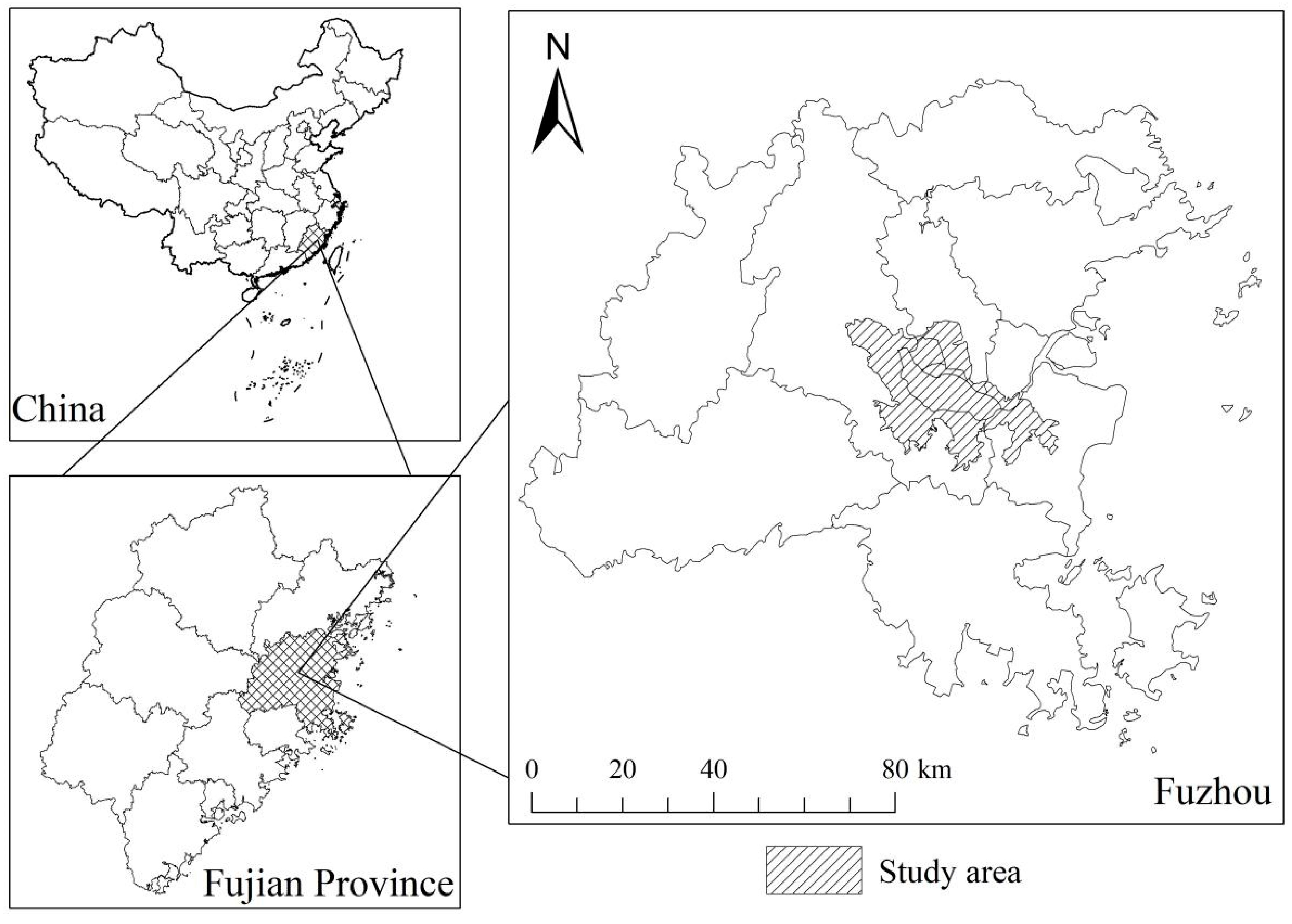
Fuzhou (25°20′ N to 26°38′ N, 118°18′ E to 119°59′ E), the capital city of Fujian province, is located in the east of Fujian province, bordering the East China Sea. It is a coastal harbour city. Fuzhou has typical estuary basin terrain with numerous mountains and hills. Fuzhou belongs to a subtropical Marine monsoon climate with a pleasant temperature and sufficient rainfall. A southerly wind prevails in summer. The annual temperature difference is minimum. The regions of this research include the main urban area of Fuzhou city and its surrounding densely populated areas, which have a total area of 698.3 km2 (Figure 1). In recent years, with the acceleration of urbanization, the urban area of Fuzhou expanded at an average annual rate of 6% to 7% from 1996 to 2005 [40]. The green area of the main urban area was small and severely fragmented [41], and it has obvious UHI [30].
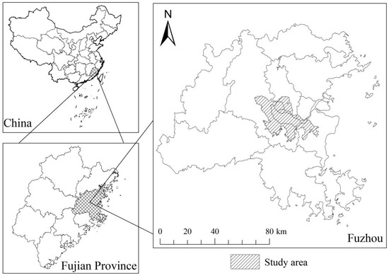
Figure 1.
Location of the study area.
3.2. Data Source and Preprocessing
The Landsat image data employed was downloaded from the Geospatial Data Cloud Platform (http://www.gscloud.cn/, accessed on 12 January 2022) of the Computer Network Information Center, Chinese Academy of Sciences. The orbit numbers of the two images are both 119/042 and the image has low cloud cover. The dates of the two images are 4 May 2000 (hereinafter referred to as the 2000 image, the data type is Landsat ETM+) and 25 June 2016 (hereinafter referred to as the 2016 image, the data type is Landsat OLI/TIRS), respectively. The “Radiometric Calibration” and “FLAASH Atmospheric Correction” tools in the Radiometric Calibration module of the ENVI 5.1 software were employed to perform data preprocessing.
3.3. Land Surface Temperature Retrieve and Urban-Heat-Island Ratio Index
In this study, the single-channel method proposed by Jiménez-Muñoz et al. [17] was used to retrieve LST. This method only needs two parameters: the surface emissivity and the total water vapour content of the atmosphere profile to perform the inversion. First, the digital values (DNs) in the thermal infrared band (Band 6 in Landsat 7 ETM+, Band 10 in Landsat 8 TIRS) were converted into the spectral emissivity values (Lλ) [Equations (1) or (2)] [30,42,43], and then we used the Equation (3) [30,42,43] to convert it into brightness temperature (Tb); additionally, the spectral emissivity was corrected according to the nature of the terrain [44,45,46].
Lλ = gain × Qcal + bias (for Landsat ETM+)
Lλ = MLQcal + AL (for Landsat TIRS)
Among them, Qcal is the DN value of the infrared band of Landsat ETM+ images; ML and AL are the adjustment factors of the infrared band of Landsat TRIS images. These are the Radiance_Mult_Band_10 and Radiance_Add_Band_10 values in the MTL header file of Landsat TRIS, which are equivalent to the gain value and offset value of the Landsat ETM+ image; for Landsat ETM+, K1 = 607.76 W/(m2·sr−1·μm−1), K2 = 1281.71 K; and for Landsat TRIS, K1 = 607.76 W/(m2·sr−1·μm−1) or 774.89 W/(m2·sr−1·μm−1), and K2 = 1281.71 K or 1321.08 K.
Using the Equation (4), Tb can be further corrected by emissivity, and then the temperature can be converted to degrees Celsius (°C) [47,48,49].
Among them, λ is the effective wavelength (for Landsat ETM+ images, while the value of λ is 11.5 μm; for Landsat TRIS images, the value of λ is 10.8 μm). ρ = 1.438 × 10⁻² mK, while ε is the surface emissivity, which can be calculated by Equation (5) [44].
Among them, m = 0.004 is the soil emissivity and n = 0.986 is the vegetation emissivity [46]. Pv is the proportion of vegetation, calculated using Equation (6). The calculation of NDVI can refer to the article of Hu et al. [50].
Since the two images used in the study area were spring image (2000) and summer image (2016), this paper adopted the method of temperature normalization [calculate using Equation (7)] [24,51] to eliminate the seasonal difference, which made the temperature values of different time phases unify to [0,1]. Then, we used the natural piecewise method to divide the normalized LST into 7 levels: extra-low temperature, low temperature, sub-low temperature, medium temperature, sub-high temperature, high temperature, and extra-high temperature, of which medium temperature area, sub-high temperature area, high-temperature area, and the extra-high temperature area were higher than the average LST of the study area, forming the heat island region. Then, the URI was proposed to calculate the ratio of the heat island to characterize the heat island effect change for the study area. The larger the URI index value, the stronger the heat island effect. The URI is expressed as Equation (8) [24].
where m is the number of surface temperature grades, which is 7 here; n is the number of regional grades of heat islands above the average surface temperature, which is 4 here; Wi is the weight value of grade i, which is equal to the temperature grade value; and Pi is the percentage of the grade i area to the total area of the study area.
3.4. Landscape Classification and Sample Designation
Taking the 2016 data as an example, combining it with the land-use characteristics of the study area, and referring to the land classification standards of the Chinese land resource classification system, the supervised classification visual interpretation method was used in the ENVI 5.1 software to classify the urban underlying land surface into three types by exploiting remote sensing images synthesized by bands (6:5:4): water, vegetation, and impervious surface (Figure 2a). The accuracy of the classification was inspected based on a confusion matrix with a total of 2088 random points. The overall classification accuracy was 98.564% and the Kappa coefficient was 0.978, respectively. The classification results showed that the proportions of the three landscapes were: water (10.837%), vegetation (27.014%), and impervious surface (62.149%), respectively.
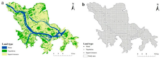

Figure 2.
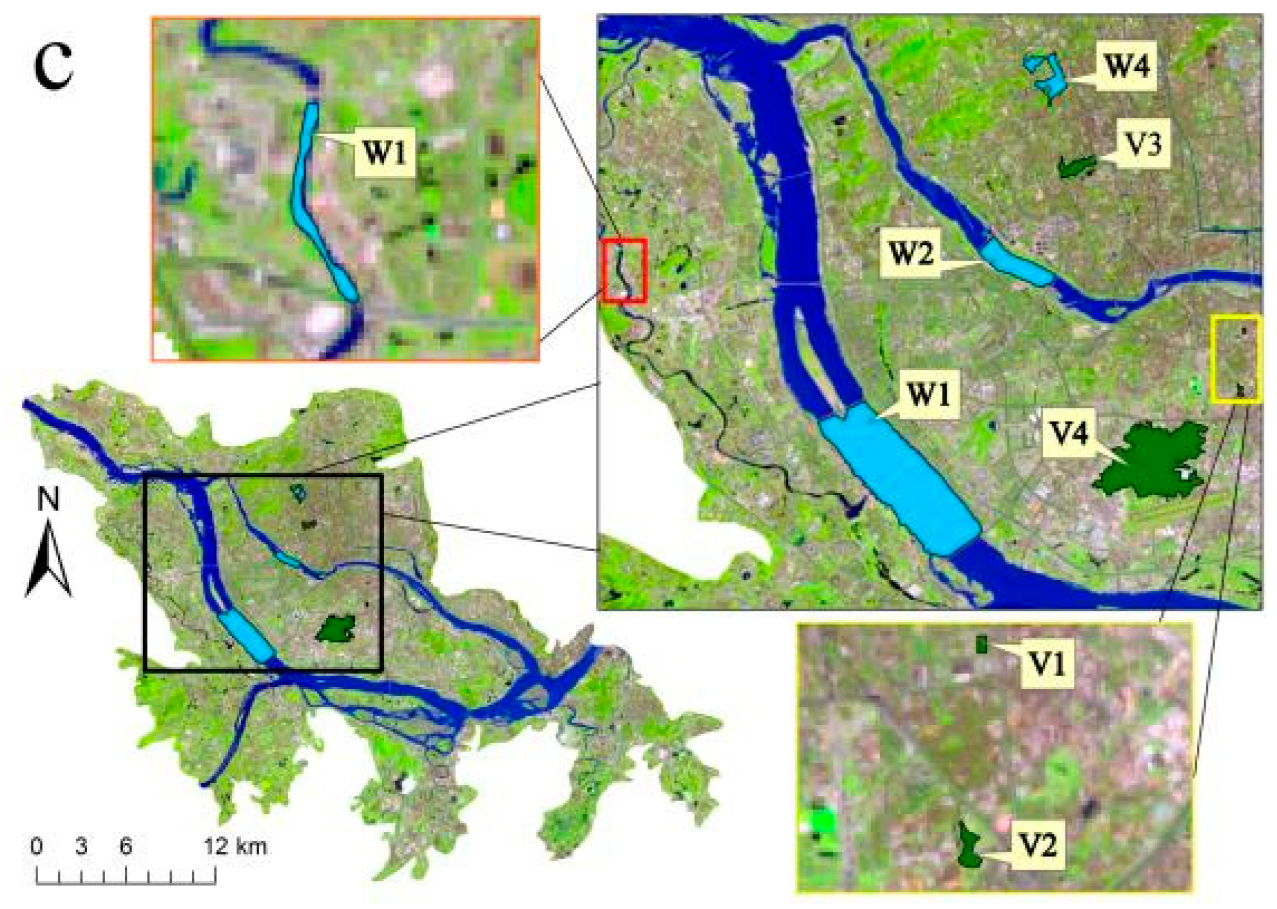
Land type and patch location in the study area. (a,b) are land types of urban underlays; (c) is patch location map of water and vegetation. Wi is the extracted water patch, Vi is the extracted vegetation patch.
Two methods were used for sampling. Firstly, a 900 m × 900 m fishnet established extract information of the temperature and the landscape type (Figure 2b), thereby allowing for the comparison of the heat environment among different landscape types. Secondly, to compare the cooling effects of water patches and vegetation patches of different sizes and shapes, four typical patches of water and vegetation were extracted according to their sizes and geographic locations based on the 2016 image, respectively (Figure 2c). The principles of extracting water bodies and green patches were: (1) patches in different sizes; (2) the environmental conditions around the sample patches were relatively consistent to reduce the disturbance of other factors. The information of the extracted patches is indicated in Table 1.

Table 1.
Water and vegetation patch sample information.
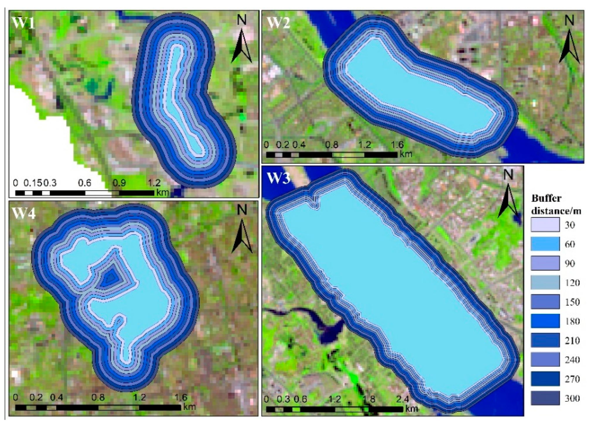
Then, ten 30 m-width buffers of each patch were created to explore the cooling effect of water area and vegetation patches of different sizes (Figure 3).
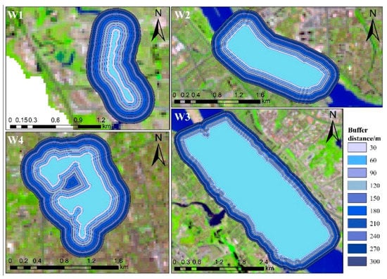
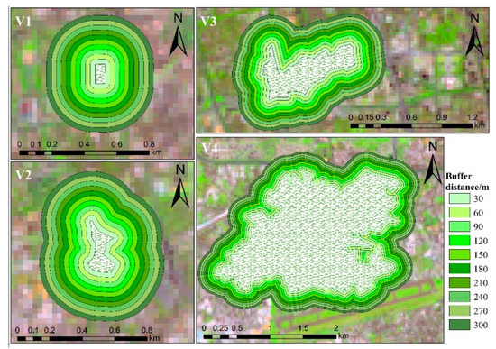
Figure 3.
Buffer image of patches of different water or vegetation.
3.5. Calculation of Landscape Pattern Comprehensive Index
3.5.1. Selection of Landscape Pattern Index
Landscape pattern refers to the type, size, shape, and spatial configuration of landscape patches. It is a quantitative indicator that describes aspects of landscape pattern information, reflecting landscape composition and configuration. In this study, the four commonly used landscape metrics (AI, Area_mn, LPI, and PLAND) were selected [52]. Then, taking the 2016 image data as a case, these metrics in each pixel were calculated adopting a moving window (900 m × 900 m) strategy in method in Fragstats 4.2 software. The calculation results of different metrics were further standardized to be between 0 and 1 using Equations (9) and (10) (Table 2). Among them, the water and vegetation had a mitigating effect on the UHI, while the increase of patches on the impervious surface exacerbated the UHI, so that the applied metrics of the water area and vegetation had a positive effect on alleviating the UHI, while metrics of the imperviousness had the opposite effect.
Table 2.
Original value and the normalized value of landscape pattern index.
3.5.2. Principal Component Analysis
We aimed to construct a comprehensive index (i.e., LPCI) that included the quantitative characteristics of all land types to quickly and quantitatively portray its cooling effects on the UHI. The effectiveness of the LPCI in practice may be affected greatly by weighting methods. In this paper, a principal components analysis (PCA) was adopted to determine the relative importance of each metric to the principal component of LPCI. PCA is a FRAGSTATS multidimensional factor compression technique, which can avoid any co-linearity problem between the four metrics [53]. PCA can automatically and objectively assign weights to each metric based on their contribution to the principal components [54,55].
Based on the above-mentioned four landscape metrics, the calculation of PCA was accomplished using the tool of “PCA Rotation” in ENVI 5.1 software. Firstly, the water landscape comprehensive index (WLCI), the vegetation landscape comprehensive index (VLCI), and the imperviousness landscape comprehensive index (ILCI) were constructed for the three main landscapes; then, the LPCI was synthesized by the WLCI, VLCI, and ILCI using PCA technique. Table 3 and Table 4 listed the statistical outcomes of all of the PCAs. All of the percent eigenvalues of PC1 were larger than 80%, indicating that the PC1 components had integrated most of the feature information of all of the metrics; thus, the PC1 was proposed to construct the final comprehensive index.
Table 3.
Principal component analysis of the comprehensive index for each landscape.
Table 4.
Principal component analysis of the overall landscape pattern comprehensive index.
3.6. Geographically Weighted Regression Model
We proposed a GWR model to explore the complex spatial variation relationship and correlation between the LPCI and the LST. GWR is a local regression technique with the ability to observe the spatial variations in the cooling effects of the LPCI on the LST, which is a significant improvement over commonly used global regression analyses (i.e., the ordinary least squares, OLS) model [56,57,58]. In this study, the GWR model was established with the LPCI as the independent variable and the LST as the dependent variable in the spatial sample unit of 900 m × 900 m. The average LST and LPCI values of each unit in 2016 were calculated based on zonal statistics of the ArcGIS 10.3 software. The GWR model formula is [59]:
In this formula, (ui, vi) represents the coordinates of the sample point; β0(ui, vi) is the slant distance; βk(ui, vi) is the regression coefficient of the k-th explanatory variable at the sample point i; and εi is the error term. The regression coefficient was estimated using local weighted least squares. The formula is:
In this formula, W(ui, vi) is the spatial weighting matrix of the observation data at the sample point i, which represents the influence of sample points around the regression point on the regression point. The closer to the sample point i, the greater the impact on the local regression parameters and the greater the weight; otherwise, the smaller the weight. The key to estimating the regression coefficient βk(ui, vi) is to calculate the spatial weight matrix. In this paper, Gauss function is used to calculate it:
where dij is the Euclidean distance between the sample point j and point i; and h is the band width, which determines the spatial variation of the GWR. The optimal bandwidth is determined by the Akaike information criterion (AIC). When AIC is at its minimum, the bandwidth h is the best.
4. Results
4.1. Spatio-Temporal Characteristics of Urban Heat Island
According to Table 5, the average LST was 35.320 °C and 39.582 °C in 2000 and 2016, respectively, which indicates a 4.262 °C increase in 16 years. From 2000 to 2016, the areas with medium temperature and below have been reduced to varying degrees. Of these, the low temperature region had the fastest decline, with its area accounting for 9.554% of the total study area; on the contrary, the high temperature region expanded fastest, with the extending area accounting for 8.709% of the total study area. As a result, the UHI area (including four temperature level regions: medium temperature, sub-high temperature, high temperature, and extra-high temperature) increased from 343.717 km2 in 2000 to 440.703 km2 in 2016, with the increased area accounting for 13.894% of the total study area.
Table 5.
Surface average temperature and temperature grade area change from 2000 to 2016.
It can be observed from Figure 4 that the area of the urban heat island was greatly expanded from 2000 to 2016. The heat island effect in the original central area of the urban had been strengthened, and it had a tendency to extend to the southeast and along the banks of the Minjiang River. Consequently, the URI value increased from 0.328 in 2000 to 0.457 in 2016, indicating an increased UHI effect in the study area.

Figure 4.
Classification of urban heat islands in 2000 and 2016.
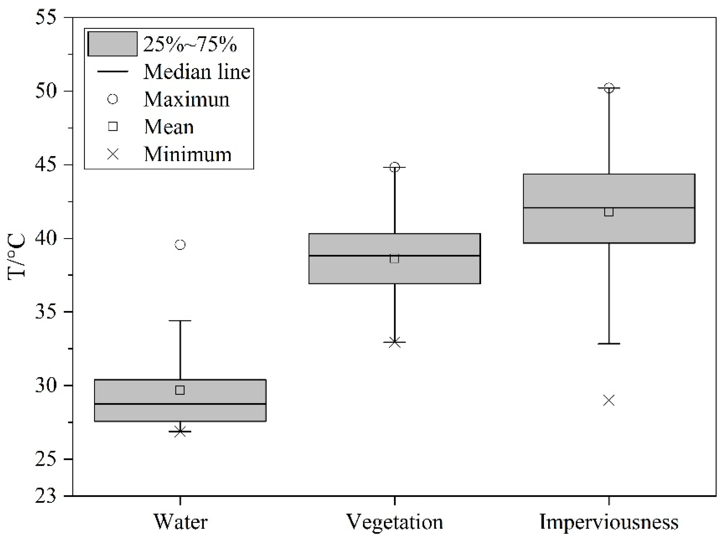
4.2. Cooling Effects of Different Landscape Types
Figure 5 indicated that the average LST of the water (29.69 °C) < the vegetation (38.56 °C) < the impervious surface (41.82 °C).
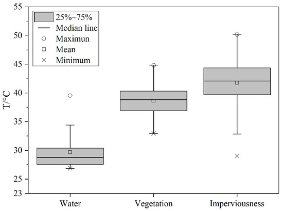
Figure 5.
Temperature of different landscape types.
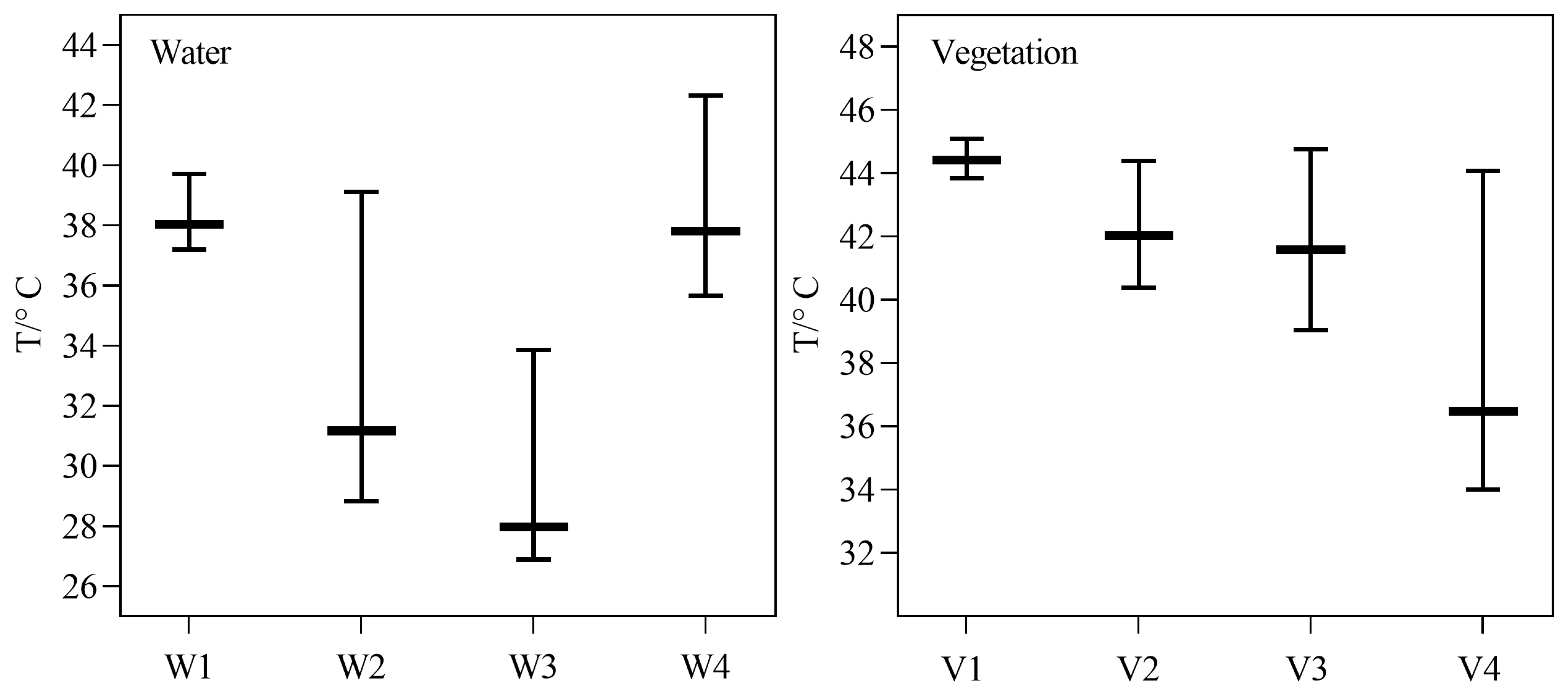
Figure 6 revealed that the temperature of the patches was inversely related to the size of the patch area, with the larger the patch area, the lower the LST. In terms of the water patches, W3 had the largest area and the lowest LST (27.97 °C), followed by the LST of W2 (31.17 °C) < W4 (37.81 °C) < W1 (38.04 °C). In terms of the vegetation patches, the order of area from largest to smallest was: V4 > V3 > V2 >V1, while the order of the LST was reversed: V4 (36.47 °C) < V3 (41.59 °C) < V2 (42.03 °C) < V1 (44.42 °C).

Figure 6.
Temperature information of water and vegetation patch samples.
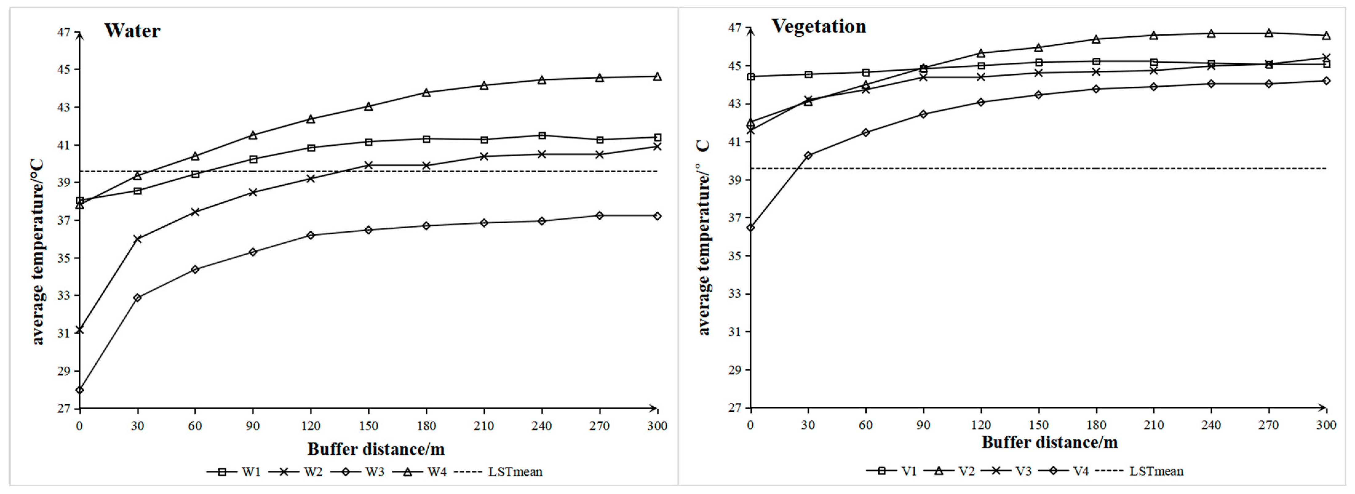
Figure 7 shows the trend of ambient LST around water and vegetation patches. In summary, the LST increased with the increase of distance, first increasing rapidly, and then increasing more gently. Figure 7 also reveals that the cooling effect of the water body patches from large to small were W3 > W2 > W1 > W4, respectively. The cooling distance of the water body patches was approximately 120–150 m, and the LST tended to be flat beyond this range. In vegetation patches, the curve of the V1 was almost flat, indicating that it has little cooling effect on the surrounding environment. The cooling distance of the other vegetation patches (i.e., V4, V3 and V2) was approximately 60–90 m. It should be noted that, although the area of four water patches was smaller than the V4, their cooling effect was greater than V4, indicating that the cooling effect of water body exceeded that of vegetation.
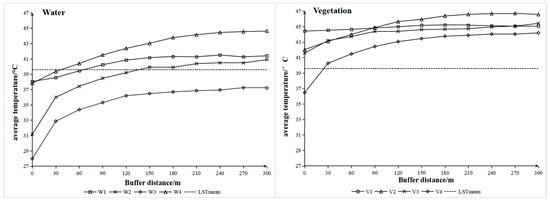
Figure 7.
Trends of LST in different distances from water (left) or vegetation (right). The temperature of each ring buffer does not include the temperature of the patch itself. The dotted line represents the average LST.
4.3. Spatial Distribution of Landscape Patterns
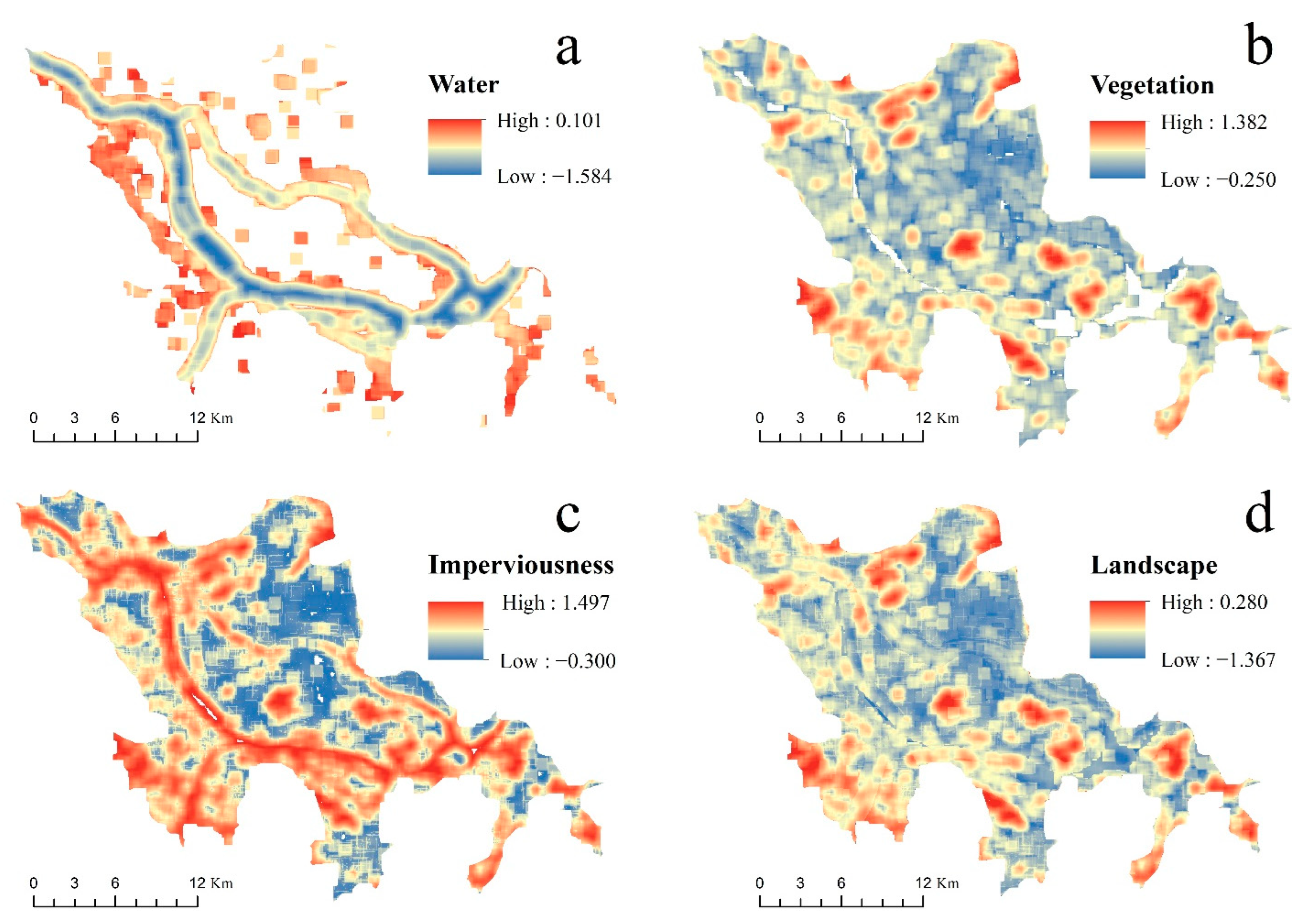
The average values of the WLCI, VLCI, and ILCI were 0.618, 0.407, and 0.490, respectively. For the water landscape, the high value of WLCI was distributed on both sides of the Minjiang river and Wulong river; additionally, some high-value clusters were distributed in the urban inland river or lake area (Figure 8a). The areas with higher VLCI value were distributed in the urban–rural junction around the study area, where there are contiguous green spaces; the hills and park areas within the urban area also had higher VLCI values (Figure 8b). Before synthesizing the ILCI (Figure 8c), its four landscape indexes had been reversely normalized. Therefore, the spatial distribution pattern of ILCI was similar to the VLCI. As a consequence, the spatial distribution pattern of LPCI was very similar to that of vegetation, with high LPCI values mainly distributed at the edge of the study area, while areas with lower values were mostly concentrated in urban centers (Figure 8d).

Figure 8.
Spatial distribution of landscape pattern. (a) is the water landscape comprehensive index; (b) is the vegetation landscape comprehensive index; (c) is the imperviousness landscape comprehensive index; (d) is the landscape pattern comprehensive index.
4.4. Spatial Heterogeneous Cooling Effects of Landscape Pattern
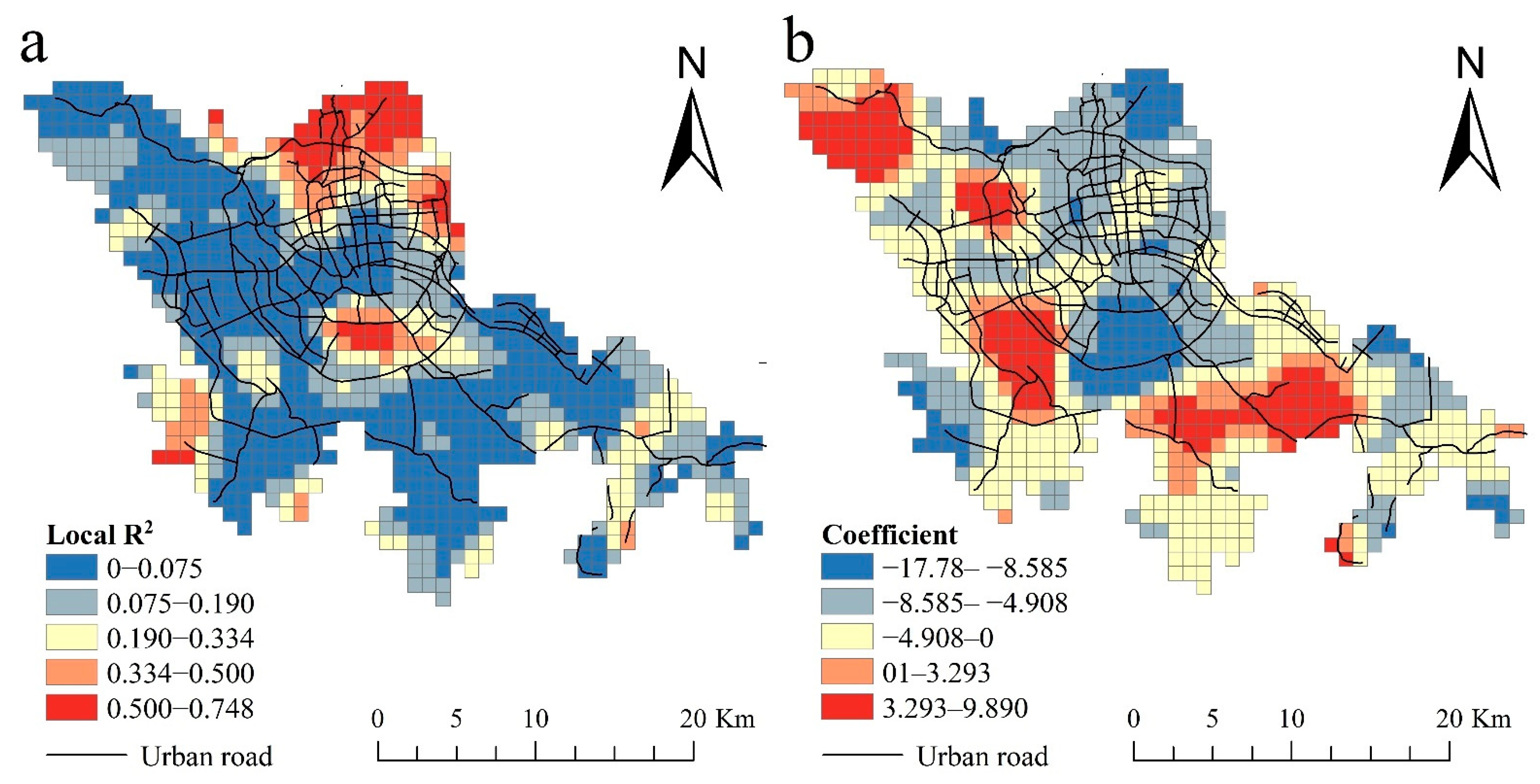
Taking LPCI as the independent variable and LST as the dependent variable, the spatial relationships between these two regressors were further studied using the GWR model. The spatial distribution of Local R2 showed that the clusters where the landscape pattern had a greater impact on the thermal environment were (the red and yellow clusters): urban centers, northern cities, and the sporadic clusters around the city (Figure 9a). Most of these clusters indicated a negative association between the LPCI and the LST (Figure 9b), suggesting that joint contributions interacting with various landscape metrics of the three major landscape types may be the predominant influencing factor for urban heat environment in these areas. This illustrates that higher AI, Area_mn, LPI, and PLAND of water area and vegetation, but lower AI, Area_mn, LPI, and PLAND of imperviousness surface, may contribute to the alleviation of the UHI. However, it should be noted that the cooling effect of the LPCI in each spatial unit was also significantly and spatially heterogeneous across the study areas. It revealed that there were a few grids that exhibited positive associations with LST (Figure 9b), though the coefficient of determination (R2) in these places was not large, most of them lower than 0.075. In this case, this suggests that the influence mechanism of these places on the thermal environment was more complicated, and the landscape pattern was not the dominant factor here.

Figure 9.
Local R2 and coefficient of GWR model. (a) is the local R2 of GWR model; (b) is the coefficient of GWR model.
5. Discussion
5.1. Validity Evaluation of LPCI
The ideal landscape index should be representative, which means that the index should fully reflect the objective characteristics of the urban landscape. In order to calculate the validity of the LPCI, the Pearson correlation test was used to evaluate the validity [50]. A two-step correlation test was performed. The first step was the correlation analysis between WLCI, VLCI, ILCI, and their constituent landscape metrics. The results showed that the average correlation coefficients were 0.913, 0.896, and 0.879, respectively, higher than any average correlation coefficients between the landscape metrics (Table 6). The second step was to test the correlation between LPCI and the comprehensive index of water, vegetation, and imperviousness (i.e., WLCI, VLCI, ILCI). The results showed that the average correlation coefficient was 0.629 (Table 7), which was also higher than average correlation coefficients between comprehensive index of water, vegetation, and imperviousness. Moreover, the significance level of all of the correlations was less than 0.01. Therefore, LPCI was considered to have a good representativeness for all of the analyzed landscape metrics of all of the landscape types.
Table 6.
Correlation matrix of three comprehensive indexes and landscape pattern index.
Table 7.
Correlation matrix of LPCI and three comprehensive indexes.
Furthermore, the results of the main component analysis showed that the first main component of WLCI, VLCI, and ILCI was greater than 85% (Table 3), while the first main component of LPCI was greater than 80% (Table 4), which means that the LPCI had the ability to explain most of the landscape pattern information. This also illustrated the objectivity and rationality of the new comprehensive index.
5.2. The Relationship between Urban Landscape and Thermal Environment
From 2000 to 2016, the UHI effect in Fuzhou showed a trend of aggravation. This was mainly due to the fact of the significant changes in land-use structure caused by the acceleration of urbanization, with the impervious surface areas of buildings and roads, among other surfaces, in the underlying of the city continually increasing, and it is difficult for water and vegetation, which only accounted for a small proportion of the total area of Fuzhou city, to mitigate the rising of LST. Moreover, due to the large urban population density and the basin terrain in the study area, the volatilization of the tremendous heat generated by human activities was very challenging. In September 2011, Fuzhou proposed to implement the urban expansion strategy of “expanding eastward and southward, along the river to the sea”. Our analysis indicated that the areas with increased thermal environment had a good consistency with this urban boundary expansion policy.
In terms of the cooling effect, we found that the cooling effect of water bodies exceeded that of vegetation, in spite of the patch area of green space being larger than that of water body. The cooling distance of the former is approximately 120–150 m, while it is about 60–90 m for the latter. Most current studies [60,61] have shown the same results as our study. Only O’Malley et al. [62] found that green spaces have a stronger cooling effect than water. Our results also verify other predecessors [63,64], which have revealed that the minimal cooling extents of the green park were generally under 100 m, but the median cooling distance can reach to 200 m.
We found that the cooling effect is affected by the size of the patch, and that the effect gradually increases as the area of the patch increases. For vegetation patches, we found that if they are too small, they have no cooling effect at all. For example, our case demonstrated that there was little cooling effect on the surrounding environment for the V1 patch, with its area less than 1 ha. This result is in line with the previous study [64], suggesting the threshold value of cooling efficiency of green spaces to be 4.55 ± 0.5 ha in Fuzhou city. Jaganmohan et al. [65] also revealed that when the size of the green space area exceeds 14 ha, the size of the green space is the primary factor influencing the cooling intensity. However, just because the patch is bigger, it does not mean that it is better. There are several reasons for this: (1) urban land resources are still relatively scarce; (2) when the patch area of urban green space is more than a certain threshold, increasing the patch area may not enhance the cooling intensity [66]; (3) optimizing greenspace configurations for fixed areas can also alleviate the UHI. For example, the cooling effect of a green space with a compact shape (such as a circle or a square) is better than that of a complex shape [67,68,69,70], while the cooling effect of the water varies with the geometry of the river, vegetation coverage, riverbank height [71,72], and climate factors [71].
There is an exception here, which is that the water area of the W4 was much larger than that of the W1, but the cooling effect of the W4 was not as good as the W1. This is because the W1 is located far from the urban center, surrounded by smaller building density, and has higher vegetation coverage, while the W4 was the West Lake in the urban center, surrounded by high-density buildings. This means that in addition to the characteristics of the patch itself, the surrounding environmental conditions will also affect its cooling effect. Our study is consistent with [71], which has found that the urban morphology around the river will affect its cooling effect, and narrow streets and lower buildings are beneficial to the river’s cooling. The river produces an effective cooling effect by dispersing cold air to the surrounding area [35,73]. Therefore, wind speed is another important factor that determines the cooling effect of water [74]. The humidity and temperature of the air are also influencing factors [72].
The shape, density, and height of buildings in the urban also influence LST [75,76,77]. Since impervious surfaces such as buildings and roads account for the heaviest proportion in urban regions, the pattern and distribution of impervious surfaces has the greatest impact on the urban thermal environment. The increase of impervious surfaces in urban regions will lead to the reduction of surface infiltration and soil moisture [78]. Couple this with the heat emission from human activities, and the LST will be raised faster than the ability of vegetation and water to alleviate urban heat environment. However, buildings have more than just an effect on raising the LST. Nichol’s [79] research found that in tropical cities, the temperature of high-rise buildings was colder than that of low-rise buildings. The research results of Cai and Xu [80] showed that a single low-rise building has a warming effect on the underlying surface of a city. However, high-rise buildings produce larger shadows, which, coupled with the impact of wind farms and greenery around the buildings, have a cooling effect on the urban surface. Building density is also an important factor affecting LST. At present, some research cases had found that building density in southern China is positively correlated with LST [81,82,83]. Moreover, the research results of Song et al. [84] showed that in northern Chinese cities, the influence of building density on LST was more obvious than in southern Chinese cities. In other different geographic environments, studies show that building density and LST may be negatively correlated. For example, in semi-arid areas, vegetation was sparse and the land was severely exposed, resulting in higher ground temperature [85,86]. The difference between the research results emphasizes the different impacts of building density on LST with different urban infrastructure conditions, population density, and environmental climates, which will lead to inconsistent or incomplete research conclusions.
Moreover, many studies have shown that the spatial configuration of landscape has a great impact on the cooling effect [67,68]. As mentioned above, we have taken an important step towards proposing a landscape comprehensive index (LPCI), which has proved to be effective and representative. Moreover, based on the GWR model, we can effectively capture the cooling effect of the LPCI on the heat environment site specifically, thus enhancing our understanding of the landscape paradigm that determines the LST at the local level. Therefore, this is conducive to the implementation of precise heat island alleviating measures, rather than a one-size-fits-all policy.
5.3. Implications and Limitations
This study revealed the relationship between LST and urban landscape pattern, so we can use this as an entry point to provide an effective way to reduce the UHI effect for urban landscape design. Firstly, water and vegetation landscape can alleviate the urban high temperature. Nevertheless, their cooling effect is affected by a variety of factors, such as area and geographic location. Secondly, the cooling effect of landscape configuration is more obvious in an urban center, where optimizing landscape configurations preferentially is encouraged. For example, we can improve the compactness of the cooling patches, through the construction of roads and riverbank greenways. In addition, expanding the existing green patch area can improve the cooling effect.
However, there are still some limitations in this study, which can be summarized as follows. Firstly, due to limited conditions, it is difficult to find patches with similar surroundings but different sizes, and there was just a small number of patches selected for analyzing the cold island effect in water and vegetation patches in this study. More patches should be selected in different sizes and geographic locations to explore the threshold size of the patch for water body and vegetation. Secondly, the cooling effect of the vegetation also depends on its tree species composition [87,88], e.g., the cooling effect of trees was higher than bushes and grass. However, this study did not make a more precise and detailed classification of vegetation. In addition, this paper only considered the impact of landscape patterns on LST; future research may integrate climate, terrain, and population density factors into the GWR model to obtain more objective and reasonable results.
6. Conclusions
This paper proposed a comprehensive index (LPCI) to evaluate landscape pattern and employed GWR to explore spatially heterogeneous in the cooling effects of the landscape. The proposed LPCI could explain more than 80% of information of all of the applied landscape metrics for all of the landscape types, which is a representative and objective index to assess urban landscape pattern. At the same time, the GWR approach could explicitly visualize the spatial heterogeneity in the cooling effects of landscape pattern and prioritize areas to optimize the landscape pattern and facilitate UHI mitigation. This study has demonstrated that, compared with vegetation patches, water patches have a more obvious cooling effect on the surrounding environment, with the cooling distance within 60–90 m for the vegetation, while reaching 120–150 m for water body. The GWR results revealed that the cooling effect of the landscape pattern varied spatially across the study area, indicating that the configuration of landscapes is more important in urban centers in alleviating urban heat environment than in urban fringe areas. The results of the research can enhance our understanding of the landscape paradigm that determines the LST and thus be conducive to the implementation of precise heat island alleviating measures. Meanwhile, this provides new ideas for future research on landscape pattern mitigation of urban heat island effect and a strong basis for landscape planning strategy.
Author Contributions
Conceptualization, S.L. and X.H.; methodology: S.L., X.L. and X.H.; validation: S.L., X.H. and J.L.; formal Analysis, S.L., L.C. and Q.Z.; data curation, S.L., X.H. and J.L.; writing—original draft: S.L.; writing—review & editing: X.H. and J.L.; project administration: C.Z., X.H. and J.L.; supervision: X.H. and J.L.; funding acquisition, C.Z., X.H. and J.L. All authors have read and agreed to the published version of the manuscript.
Funding
The research was supported by the National Natural Science Foundation of China (Grant No. 31971639), the General Project of Fujian Natural Science Foundation (Grant No. 2019J01406), the Leading Key Technology Projects in the Transportation Technology Market in Fujian Province (Grant No. 201823), and the Forestry Summit Discipline Construction Project of Fujian Agricultural and Forestry University (Grant No. 71201800705).
Institutional Review Board Statement
Not applicable.
Informed Consent Statement
Not applicable.
Data Availability Statement
The data presented in this study are available on request from the corresponding author.
Conflicts of Interest
The authors declare no conflict of interest.
References
- Wei, H.K.; Li, L.; Nian, M. Strategy and Policy of China’s Urbanization during the 14th Five Year Period. J. Party Sch. Cent. Comm. CPC 2020, 24, 5–21. [Google Scholar] [CrossRef]
- Hou, H.R.; Ding, F.; Li, Q.S. Remote Sensing Analysis of Changes of Urban Thermal Environment of Fuzhou City in China in the Past 20 Years. J. Geo-Inf. Sci. 2018, 20, 385–395. [Google Scholar]
- Chen, Y.H.; Cai, Y.B. The differences of thermal environment effect of urban green space evolution: A case study of Fuzhou. Chin. J. Ecol. 2019, 38, 2149–2158. [Google Scholar]
- Fan, Z.Y.; Zhan, Q.M.; Liu, H.M.; Yang, C.; Xia, Y. Spatial-temporal Distribution of Urban Heat Island and the Heating Effect of Impervious Surface in Summer in Wuhan. J. Geo-Inf. Sci. 2019, 21, 226–235. [Google Scholar]
- Zhang, X.L.; Zhao, P.X.; Gao, L.H.; Zhao, X.; Wang, H. Analysis of Heat Island Effect Based on Landsat Images in Xining City. J. Northwest For. Univ. 2016, 31, 183–190. [Google Scholar]
- Liu, Y.H.; Xu, Y.M.; Ma, J.J.; Quan, W.J. Quantitative Assessment and Planning Simulation of Beijing Urban Heat Island. Ecol. Environ. Sci. 2014, 23, 1156–1163. [Google Scholar]
- Buyantuyev, A.; Wu, J.G. Urban heat islands and landscape heterogeneity: Linking spatiotemporal variations in surface temperatures to land-cover and socioeconomic patterns. Landsc. Ecol. 2010, 25, 17–33. [Google Scholar] [CrossRef]
- Cui, L.L.; Li, G.S.; Ji, D.J. Heat island effect and its relationship with land use in Chengdu City. Chin. J. Ecol. 2013, 37, 1518–1526. [Google Scholar]
- Li, D.; Bou-Zeid, E. Synergistic Interactions between Urban Heat Islands and Heat Waves: The Impact in Cities Is Larger than the Sum of Its Parts. J. Appl. Meteorol. Climatol. 2013, 52, 2051–2064. [Google Scholar] [CrossRef] [Green Version]
- Qiu, X.F.; Gu, L.H.; Zeng, Y.; Jiang, A.J.; He, Y.J. Study on Urban Heat Island Effect of Nanjing. Clim. Environ. Res. 2008, 13, 807–814. [Google Scholar]
- Wang, L.; Xu, H.Q. Thermal Environment Change of Fuzhou City with Rapid Urbanization. J. Tongji Univ. 2017, 45, 1336–1344. [Google Scholar]
- Shou, Y.X.; Zhang, D.L. Recent advances in understanding urban heat island effects with some future prospects. Acta Meteorol. Sin. 2012, 70, 338–353. [Google Scholar]
- Xie, Q.J.; Liu, J.H.; Hu, D.H. Urban expansion and its impact on spatio-temporal variation of urban thermal characteristics: A case study of Wuhan. Geogr. Res. 2016, 35, 1259–1272. [Google Scholar]
- Yao, Y.; Chen, X.; Qian, J. Research progress on the thermal environment of the urban surfaces. Acta Ecol. Sin. 2018, 38, 1134–1147. [Google Scholar]
- Le, T.C.; Nie, S.; Pan, H.; Li, L.C. Land surface temperature retrieval and urban heat island effect based on Landsat 8 image in Fuzhou city. J. Northwest For. Univ. 2019, 34, 154–160. [Google Scholar]
- Li, F.J.; Ma, A.Q.; Ding, Y.D.; Yang, J.J.; Jiao, J.C.; Liu, L.J. Research on Urban Heat Island Effect Based on Landsat Data. Remote Sens. Technol. Appl. 2009, 24, 553–558. [Google Scholar]
- Jimenez-Munoz, J.C.; Sobrino, J.A. A Generalized Single Channel method for retrieving land surface temperature from remote sensing data. J. Geophys. Res. 2003, 108, 4688–4697. [Google Scholar] [CrossRef] [Green Version]
- Qin, Z.; Karnieli, A.; Berliner, P. A Mono-Window Algorithm for Retrieving Land Surface Temperature from Landsat TM Data and Its Application to the Israel Egypt Border Region. Int. J. Remote Sens. 2001, 22, 3719–3746. [Google Scholar] [CrossRef]
- Sobrino, J.A.; Li, Z.L.; Stoll, M.P.; Becker, F. Multi-channel and multi-angle algorithms for estimating sea and land surface temperature with ATSR data. Int. J. Remote Sens. 1996, 17, 2089–2114. [Google Scholar] [CrossRef]
- Tan, Z.H.; Zhang, M.H.; Karnieli, A.; Berliner, P. Mono-window Algorithm for Retrieving Land Surface Temperature from Landsat TM6 data. Acta Geogr. Sin. 2001, 4, 456–466. [Google Scholar]
- Yang, M.; Yang, G.A.; Wang, Y.J.; Zhang, Y.F.; Zhang, Z.H.; Sun, C.H. Remote sensing analysis of temporal-spatial variations of urban heat island effect over Beijing. Remote Sens. Land Resour. 2018, 30, 213–223. [Google Scholar]
- Wang, T.X.; Chen, S.L.; Yan, G.J. Estimation of land surface parameters and spatio-temporal characteristics of urban heat island. Sci. Geogr. Sin. 2009, 29, 697–702. [Google Scholar]
- Su, Y.L.; Zhang, Y.F. Spatio-temporal characteristics of urban heat island effect of Xi′an city based on landsat TM/ETM+. Bull. Soil Water Conserv. 2011, 31, 230–234. [Google Scholar]
- Xu, H.Q.; Chen, B.Q. A study on urban heat island and its spatial relationship with urban expansion: Xiamen, SE, China. Urban Dev. Stud. 2004, 11, 65–70. [Google Scholar]
- Liu, Y.H.; Fang, X.Y.; Zhang, S.; Luan, Q.Z.; Quan, W.J. Research on quantitative evaluations of heat islands for the Beijing-Tianjin-Hebei urban agglomeration. Acta Ecol. Sin. 2017, 37, 5818–5835. [Google Scholar]
- Sun, M.; Xie, M.; Ding, M.H.; Xu, W.L.; Huang, S.Q.; Gao, F. Spatio-temporal variation of urban heat island effects in Fangchenggang City, Guangxi Zhuang Autonomos Region. Remote Sens. Land Resour. 2018, 30, 135–143. [Google Scholar]
- Xue, W.R.; Lu, Z.; Dan, S.Z.; Xu, H.X.; He, Z.W.; Chou, W.X. Evaluation of urban heat island effects in Neijiang City of Sichuan province based on thermal infrared remote sensing. Geomat. Spat. Inf. Technol. 2012, 35, 38–41. [Google Scholar]
- He, J.J.; Yu, Y.; Yu, L.J.; Liu, N.; Zhao, S.P. Impacts of uncertainty in land surface information on simulated surface temperature and precipitation over China. Int. J. Climatol. 2017, 37, 829–847. [Google Scholar] [CrossRef]
- Li, Y.L.; Wang, X.Q.; Chen, Y.Z.; Wang, M.M. The correlation analysis of land surface temperature and fractional vegetation coverage in Fujian province. J. Geo-Inf. Sci. 2019, 21, 445–454. [Google Scholar]
- Xu, H.Q. Quantitative analysis on the relationship of urban impervious surface with other components of the urban ecosystem. Acta Ecol. Sin. 2009, 29, 2456–2462. [Google Scholar]
- Zhang, C.S.; Xie, G.D.; Lu, C.X.; Liu, C.L.; Li, N.; Wang, S.; Sun, Y.Z. The mitigating effects of different urban green lands on the heat island effect in Beijing. Resour. Sci. 2015, 37, 1156–1165. [Google Scholar]
- Grover, A.; Singh, R. Analysis of Urban Heat Island (UHI) in relation to normalized difference vegetation index (NDVI): A comparative study of Delhi and Mumbai. Environments 2015, 2, 125–138. [Google Scholar] [CrossRef] [Green Version]
- Hu, Y.H.; Jia, G.S. Influence of land use change on urban heat island derived from multi-sensor data. Int. J. Climatol. 2010, 30, 1382–1395. [Google Scholar] [CrossRef]
- Klok, L.; Zwart, S.; Verhagen, H.; Mauri, E. The surface heat island of Rotterdam and its relationship with urban surface characteristics. Resour. Conserv. Recycl. 2012, 64, 23–29. [Google Scholar] [CrossRef]
- Saaroni, H.; Ziv, B. The impact of a small lake on heat stress in a Mediterranean urban park: The case of Tel Aviv, Israel. Int. J. Biometeorol. 2003, 47, 156–165. [Google Scholar] [CrossRef]
- Sun, R.H.; Chen, A.L.; Chen, L.D.; Lü, Y.H. Cooling effects of wetlands in an urban region: The case of Beijing. Ecol. Indic. 2012, 20, 57–64. [Google Scholar] [CrossRef]
- Peng, J.; Liu, Y.X.; Shen, H.; Xie, P.; Hu, X.X.; Wang, Y.L. Using impervious surfaces to detect urban expansion in Beijing of China in 2000s. Chin. Geogr. Sci. 2016, 26, 229–243. [Google Scholar]
- Myint, S.W.; Brazel, A.; Okin, G.; Buyantuyev, A. Combined Effects of impervious surface and vegetation cover on air temperature variations in a rapidly expanding desert City. GIScience Remote Sens. 2010, 47, 301–320. [Google Scholar] [CrossRef]
- Li, B.; Shi, X.M.; Wang, H.Y.; Qin, M.Z. Analysis of the relationship between urban landscape patterns and thermal environment: A case study of Zhengzhou City, China. Ecol. Environ. Conserv. 2020, 192, 540. [Google Scholar] [CrossRef]
- Wang, L.; Xu, H.Q.; Li, S. Dynamic Monitoring of the Urban Expansion in Fuzhou of SE China Using Remote Sensing Technology. J. Geo-Inf. Sci. 2006, 29, 693–700. [Google Scholar]
- Lan, S.R.; Tang, S.S.; Zhang, X.P.; Xiao, S.; Zhang, X.Y.; Chen, J.X.; Huang, X.W. Fuzhou landscape pattern and urban forest system based on remote sensing data. J. Chin. Urban For. 2009, 7, 4–7. [Google Scholar]
- Chander, G.; Markham, B.L.; Helder, D.L. Summary of current radio metric calibration coefficients for Landsat MSS, TM, ETM+, and EO-1 ALI sensors. Remote Sens. Environ. 2009, 113, 893–903. [Google Scholar] [CrossRef]
- United States Geological Survey (USGS). Landsat 8 (L8) Data Users Handbook; U.S. Geological Survey: Reston, VA, USA, 2016.
- Sobrino, J.A.; Jiménez-Muñoz, J.C.; Paolini, L. Land surface temperature retrieval from Landsat TM 5. Remote Sens. Environ. 2004, 90, 434–440. [Google Scholar] [CrossRef]
- Weng, Q. Thermal infrared remote sensing for urban climate and environmental studies: Methods, applications, and trends. ISPRS J. Photogramm. Remote Sens. 2009, 64, 335–344. [Google Scholar] [CrossRef]
- Xu, H.Q.; Huang, S.L.; Zhang, T.J. Built-up land mapping capabilities of the aster and Landsat ETM+ sensors in coastal areas of south eastern China. Adv. Space Res. 2013, 52, 1437–1449. [Google Scholar] [CrossRef]
- Artis, D.A.; Carnahan, W.H. Survey of emissivity variability in thermography of urban areas. Remote Sens. Environ. 1982, 12, 313–329. [Google Scholar] [CrossRef]
- Estoque, R.C.; Murayama, Y.; Myint, S.W. Effects of landscape composition and pattern on land surface temperature: An urban heat island study in the megacities of Southeast Asia. Sci. Total Environ. 2017, 577, 349–359. [Google Scholar] [CrossRef]
- Weng, Q.; Lu, D.; Schubring, J. Estimation of land surface temperature-vegetation abundance relationship for urban heat island studies. Remote Sens. Environ. 2004, 89, 467–483. [Google Scholar] [CrossRef]
- Hu, X.S.; Xu, H.Q. A new remote sensing index based on the pressure-state-response framework to assess regional ecological change. Environ. Sci. Pollut. Res. 2019, 26, 5381–5393. [Google Scholar] [CrossRef]
- Lin, Z.L.; Xu, H.Q. Comparative Study on the Urban Heat Island Effect in “Stove Cities” during the Last 20 Years. Remote Sens. Technol. Appl. 2019, 34, 521–530. [Google Scholar]
- Guo, G.; Wu, Z.; Cao, Z.; Chen, Y.; Zheng, Z. Location of greenspace matters: A new approach to investigating the effect of the greenspace spatial pattern on urban heat environment. Landsc. Ecol. 2021, 36, 1533–1548. [Google Scholar] [CrossRef]
- Seddon, A.W.R.; Macias-Fauria, M.; Long, P.R.; Benz, D.; Willis, K.J. Sensitivity of global terrestrial ecosystems to climate variability. Nature 2016, 531, 229–232. [Google Scholar] [CrossRef] [Green Version]
- Feng, X.G.; Sai, L.W.; Shi, H. Study on the urban heat island effect based on the PCA of multi-purpose—Taking Xi′an city as an example. J. Xi′Univ. Archit. Technol. 2012, 44, 507–511. [Google Scholar]
- Xu, H.Q.; Wang, M.Y.; Shi, T.T.; Guan, H.D.; Fang, C.Y.; Lin, Z.L. Prediction of ecological effects of potential population and impervious surface increases using a remote sensing based ecological index (RSEI). Ecol. Indic. 2018, 93, 730–740. [Google Scholar] [CrossRef]
- Pan, H.; Jiang, Z.L.; Zhang, B.Y. Geographically weighted regression-based research on the spatial relationship of the influence of urban land use on land surface temperature. J. For. Environ. 2019, 39, 165–173. [Google Scholar]
- Tang, Y.Q.; Xu, W.; Ai, F.L. A GWR-Based Study on Spatial Pattern and Structural Determinants of Shanghai′s Housing Price. Econ. Geogr. 2012, 32, 52–58. [Google Scholar]
- Jiang, Z.L.; Yang, S.Y.; Sha, J.M. Application of GWR model in hyperspectral prediction of soil heavy metals. Acta Geogr. Sin. 2017, 72, 533–544. [Google Scholar]
- Brunsdon, C.; Fotheringham, S.; Charlton, M. Geographically Weighted Regression. J. R. Stat. Soc. Ser. D-Stat. 1998, 47, 431–443. [Google Scholar] [CrossRef]
- Yu, Z.W.; Guo, Q.H.; Sun, R.H. Impact of urban cooling effect based on landscape scale: A review. Chin. J. Appl. Ecol. 2015, 26, 636–642. [Google Scholar]
- Yang, G.; Yu, Z.; Jørgensen, G.; Vejre, H. How can urban blue-green space be planned for climate adaption in high- latitude cities? A seasonal perspective. Sustain. Cities Soc. 2020, 53, 101932. [Google Scholar] [CrossRef]
- O’Malley, C.; Piroozfar, P.; Farr, E.R.; Pomponi, F. Urban Heat Island (UHI) mitigating strategies: A case-based comparative analysis. Sustain. Cities Soc. 2015, 19, 222–235. [Google Scholar] [CrossRef] [Green Version]
- Lin, W.; Yu, T.; Chang, X.; Wu, W.; Zhang, Y. Calculating cooling extents of green parks using remote sensing: Method and test. Landsc. Urban Plan. 2015, 134, 66–75. [Google Scholar] [CrossRef]
- Yu, Z.; Guo, X.; Zeng, Y.; Koga, M.; Vejre, H. Variations in land surface temperature and cooling efficiency of green space in rapid urbanization: The case of Fuzhou city, China. Urban Urban Green 2018, 29, 113–121. [Google Scholar] [CrossRef]
- Jaganmohan, M.; Knapp, S.; Buchmann, C.M.; Schwarz, N. The bigger, the better? The influence of urban green space design on cooling effects for residential areas. J. Environ. Qual. 2016, 45, 134–145. [Google Scholar] [CrossRef]
- Zhou, W.; Shen, X.; Cao, F.; Sun, Y. Effects of area and shape of greenspace on urban cooling in Nanjing, China. J. Urban Plan. Dev. 2019, 145, 04019016. [Google Scholar] [CrossRef]
- Chen, A.; Yao, L.; Sun, R.; Chen, L. How many metrics are required to identify the effects of the landscape pattern on land surface temperature? Ecol. Ind. 2014, 45, 424–433. [Google Scholar] [CrossRef]
- Debbage, N.; Shepherd, J.M. The urban heat island effect and city contiguity. Comput. Environ. Urban Syst. 2015, 54, 181–194. [Google Scholar] [CrossRef]
- Martins, T.A.; Adolphe, L.; Bonhomme, M.; Guyard, W. Impact of urban cool Island measures on outdoor climate and pedestrian comfort: Simulations for a new district of Toulouse, France. Sustain. Cities Soc. 2016, 26, 9–26. [Google Scholar] [CrossRef]
- Sun, R.; Xie, W.; Chen, L. A landscape connectivity model to quantify contributions of heat sources and sinks in urban regions. Landsc. Urban Plan. 2018, 178, 43–50. [Google Scholar] [CrossRef]
- Park, C.Y.; Lee, D.K.; Asawa, T.; Murakami, A.; Kim, H.G.; Lee, M.K.; Lee, S.H. Influence of urban form on the cooling effect of a small urban river. Landsc. Urban Plan. 2019, 183, 26–35. [Google Scholar] [CrossRef]
- Du, H.; Song, X.; Jiang, H.; Kan, Z.; Wang, Z.; Cai, Y. Research on the cooling island effects of water body: A case study of Shanghai, China. Ecol. Indic. 2016, 67, 31–38. [Google Scholar] [CrossRef]
- Kim, D.; Cha, J.; Jung, E. A study on the impact of urban river refurbishment to the thermal environment of surrounding residential area. J. Environ. Prot. 2014, 5, 454–465. [Google Scholar] [CrossRef] [Green Version]
- Tominaga, Y.; Sato, Y.; Sadohara, S. CFD simulations of the effect of evaporative cooling from water bodies in a micro-scale urban environment: Validation and application studies. Sustain. Cities Soc. 2015, 19, 259–270. [Google Scholar] [CrossRef]
- Li, W.; Bai, Y.; Chen, Q.; He, K.; Ji, X.; Han, C. Discrepant impacts of land use and land cover on urban heat islands: A case study of Shanghai, China. Ecol. Indic. 2014, 47, 171–178. [Google Scholar] [CrossRef]
- Sun, R.; Lü, Y.; Chen, L.; Yang, L.; Chen, A. Assessing the stability of annual temperatures for different urban functional zones. Build. Environ. 2013, 65, 90–98. [Google Scholar] [CrossRef]
- Zheng, B.; Myint, S.W.; Fan, C. Spatial configuration of anthropogenic land cover impacts on urban warming. Landsc. Urban Plan. 2014, 130, 104–111. [Google Scholar] [CrossRef]
- Li, X.; Kamarianakis, Y.; Ouyang, Y.; Turner Ii, B.L.; Brazel, A. On the association between land system architecture and land surface temperatures: Evidence from a Desert Metropolis—Phoenix, Arizona, U.S.A. Landsc. Urban Plan. 2017, 163, 107–120. [Google Scholar] [CrossRef] [Green Version]
- Nichol, J.E. High-resolution surface temperature patterns related to urban morphology in a tropical city: A satellite-based study. J. Appl. Meteorol. 1996, 35, 135–146. [Google Scholar] [CrossRef] [Green Version]
- Cai, H.; Xu, X. Impacts of built-up area expansion in 2D and 3D on regional surface temperature. Rev. Sustain. 2017, 9, 1862. [Google Scholar] [CrossRef] [Green Version]
- Du, H.; Wang, D.; Wang, Y.; Zhao, X.; Qin, F.; Jiang, H.; Cai, Y. Influences of land cover types, meteorological conditions, anthropogenic heat and urban area on surface urban heat island in the Yangtze River Delta Urban Agglomeration. Sci. Total Environ. 2016, 571, 461–470. [Google Scholar] [CrossRef]
- Li, J.; Song, C.; Cao, L.; Zhu, F.; Meng, X.; Wu, J. Impacts of landscape structure on surface urban heat islands: A case study of Shanghai, China. Remote Sens. Environ. 2011, 115, 3249–3263. [Google Scholar] [CrossRef]
- Peng, J.; Jia, J.; Liu, Y.; Li, H.; Wu, J. Seasonal contrast of the dominant factors for spatial distribution of land surface temperature in urban areas. Remote Sens. Environ. 2018, 215, 255–267. [Google Scholar] [CrossRef]
- Song, J.C.; Chen, W.; Zhang, J.J.; Huang, K.; Hou, B.Y.; Prishchepov, A.V. Effects of building density on land surface temperature in China: Spatial patterns and determinants. Landsc. Urban Plan. 2020, 198, 103794. [Google Scholar] [CrossRef]
- Azhdari, A.; Soltani, A.; Alidadi, M. Urban morphology and landscape structure effect on land surface temperature: Evidence from Shiraz, a semi-arid city. Sustain. Cities Soc. 2018, 41, 853–864. [Google Scholar] [CrossRef]
- Mathew, A.; Khandelwal, S.; Kaul, N. Spatio-temporal variations of surface temperatures of Ahmedabad city and its relationship with vegetation and urbanization parameters as indicators of surface temperatures. Remote Sens. Appl. Soc. Environ. 2018, 11, 119–139. [Google Scholar] [CrossRef]
- Kong, F.H.; Yin, H.W.; James, P.; Hutyra, L.R.; He, H.S. Effects of spatial pattern of greenspace on urban cooling in a large metropolitan area of eastern China. Landsc. Urban Plan. 2014, 128, 35–47. [Google Scholar] [CrossRef]
- Demuzere, M.; Orru, K.; Heidrich, O.; Faehnle, M. Mitigating and adapting to climate change: Multi-functional and multi-scale assessment of green urban infrastructure. J. Environ. Manag. 2014, 146, 107–115. [Google Scholar] [CrossRef]


Publisher’s Note: MDPI stays neutral with regard to jurisdictional claims in published maps and institutional affiliations. |
© 2022 by the authors. Licensee MDPI, Basel, Switzerland. This article is an open access article distributed under the terms and conditions of the Creative Commons Attribution (CC BY) license (https://creativecommons.org/licenses/by/4.0/).