
Coastal Wetland Vegetation Classification Using Pixel-Based, Object-Based and Deep Learning Methods Based on RGB-UAV
 ,
, 
Abstract
1. Introduction
2. Materials and Methods
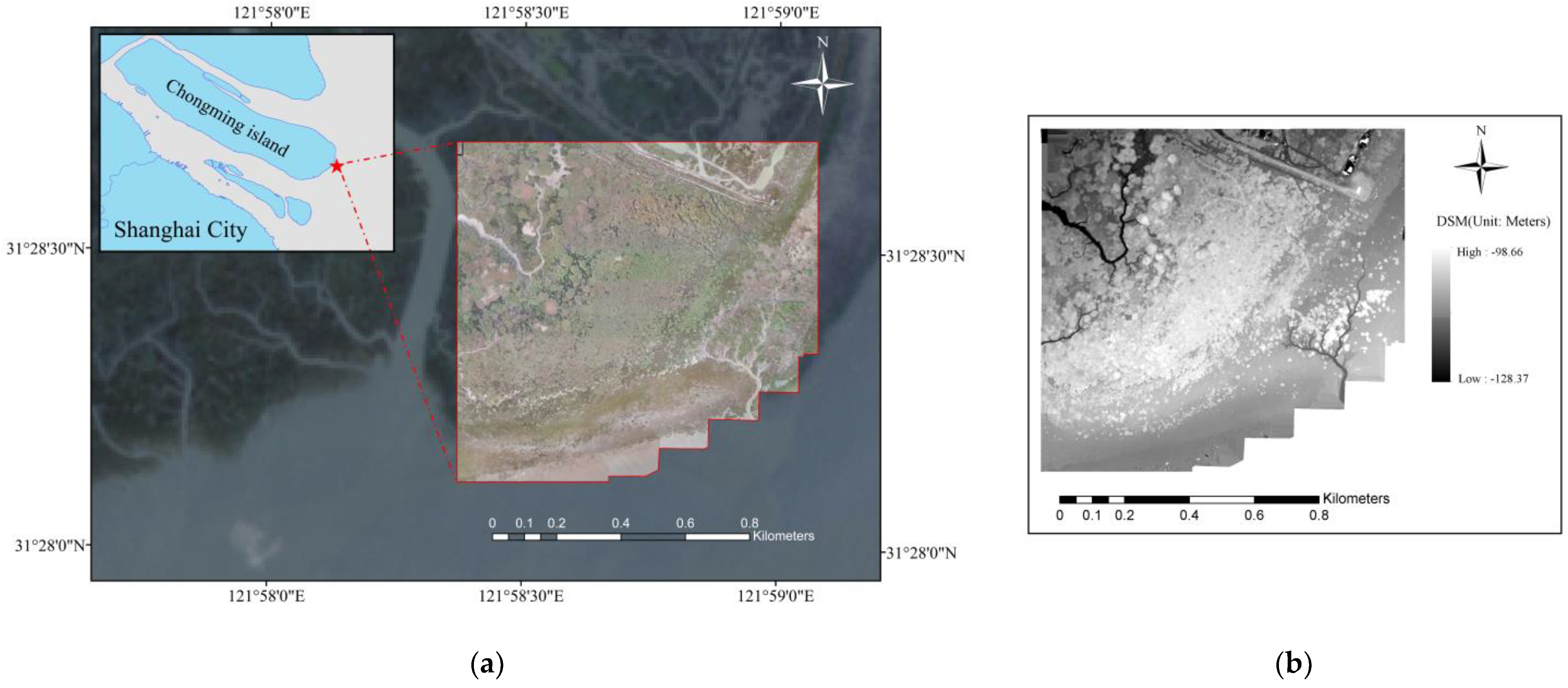
2.1. Study Area
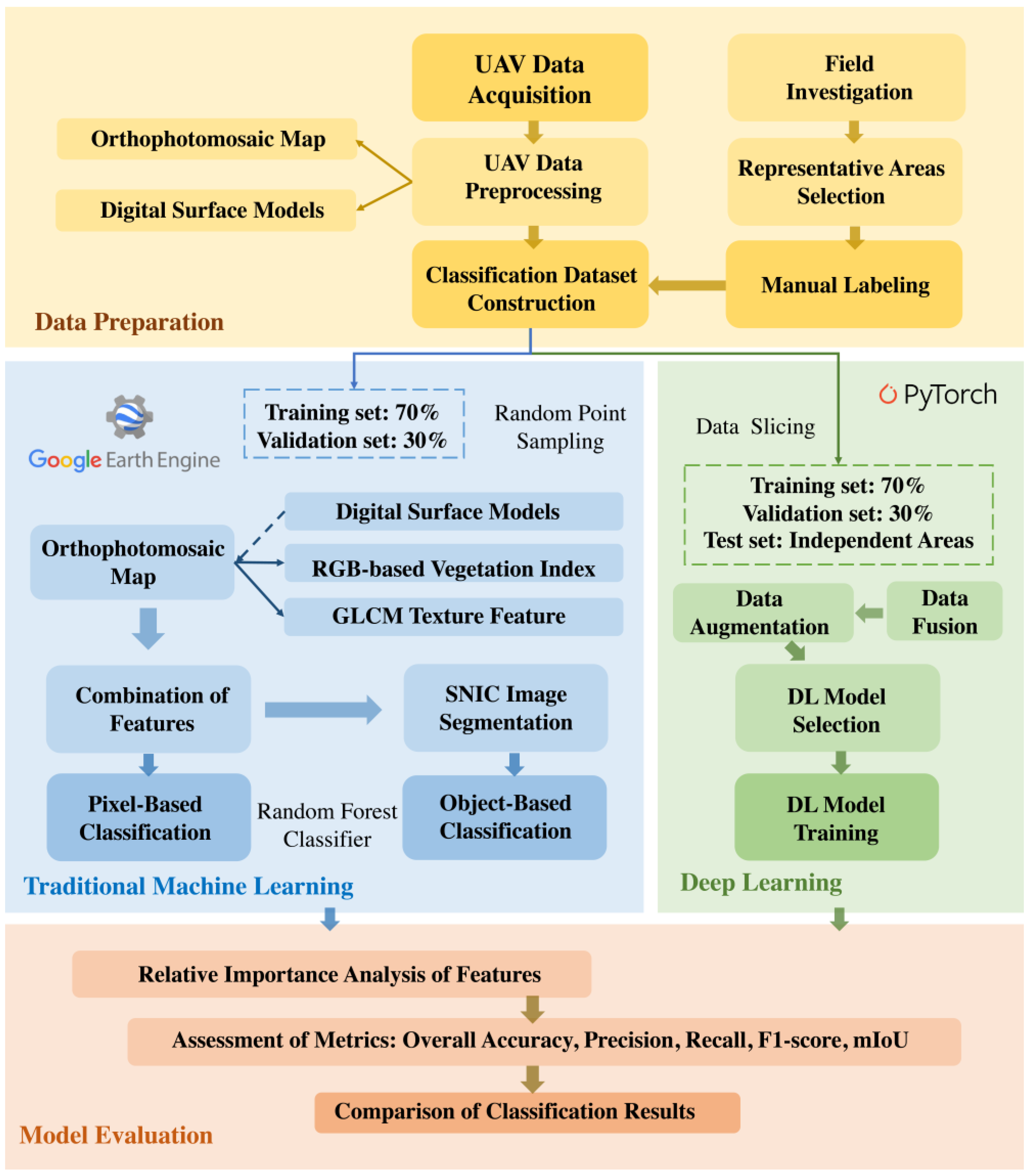
2.2. Study Workflow
2.3. Data Preparation
2.3.1. UAV Data Acquisition and Preprocessing
2.3.2. Construction of Coastal Wetland Vegetation Dataset
2.4. PB and OBIA Classification in GEE
2.4.1. RGB-Based Vegetation Index Extraction
2.4.2. Texture Feature Extraction
2.4.3. Image Segmentation in GEE
2.4.4. Random Forest Classifier and Feature Relative Importance Analysis
2.5. Deep Learning
2.5.1. Data Slicing and Data Augmentation
2.5.2. Training of DL Models
2.6. Accuracy Evaluation Metrics
3. Results
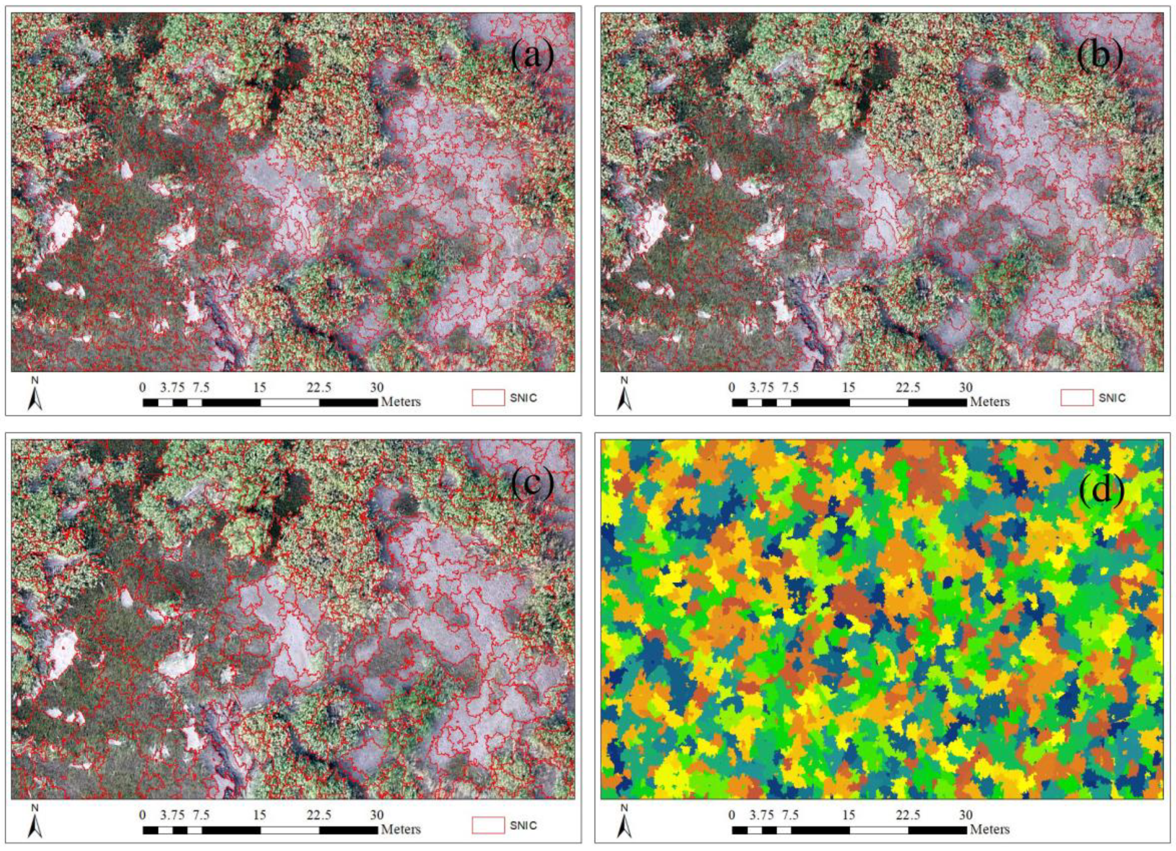
3.1. Image Segmentation Results Based on SNIC Algorithm in GEE
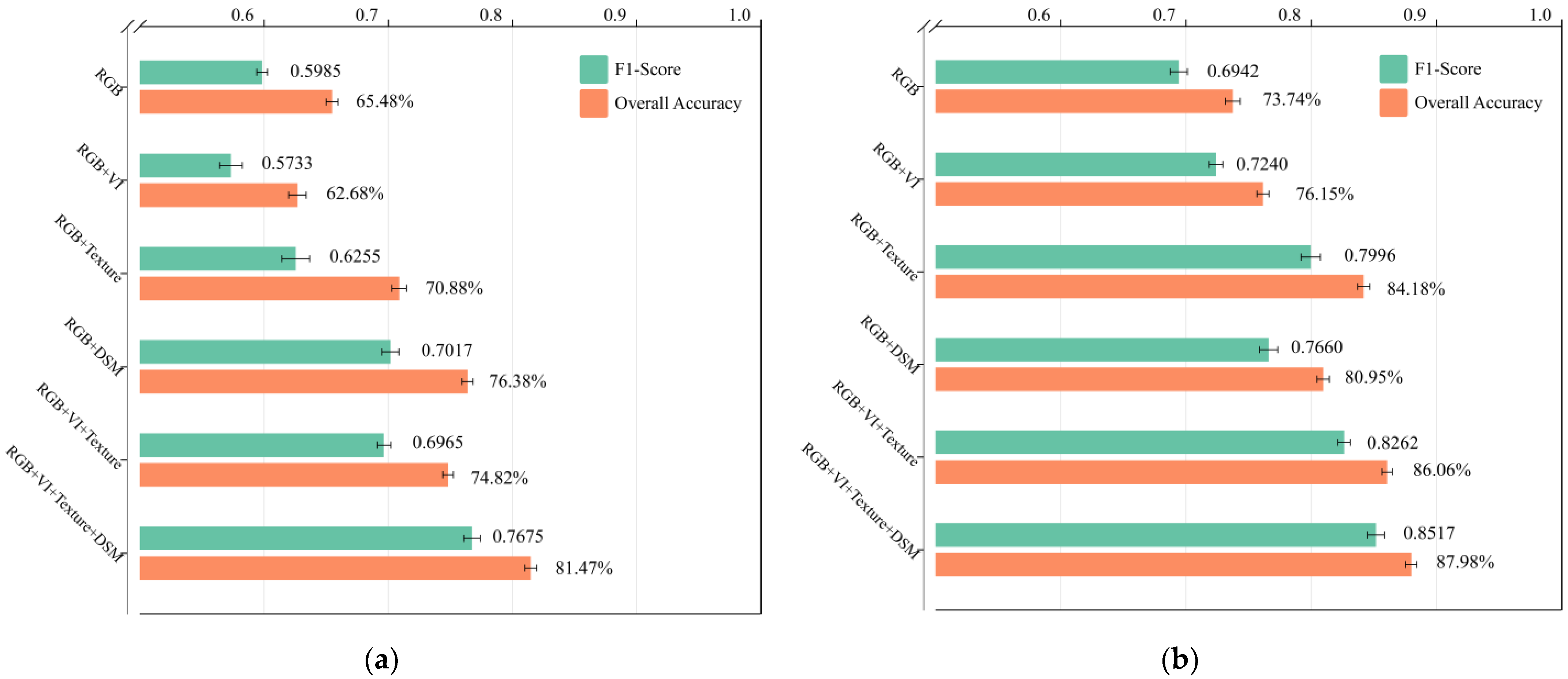
3.2. Results of PB and OBIA Classification under Different Feature Engineering
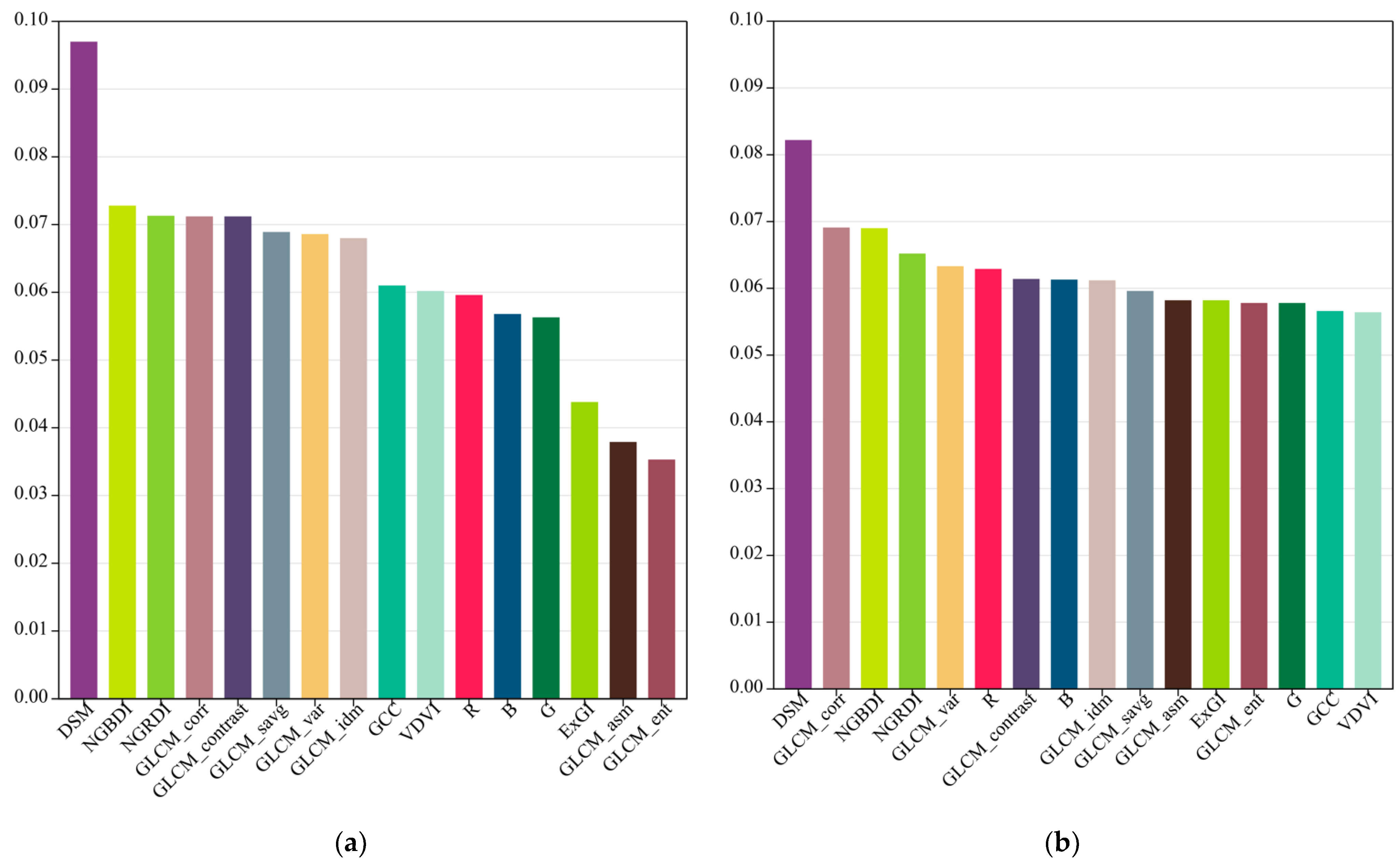
3.3. Relative Feature Importance in PB and OBIA Classification
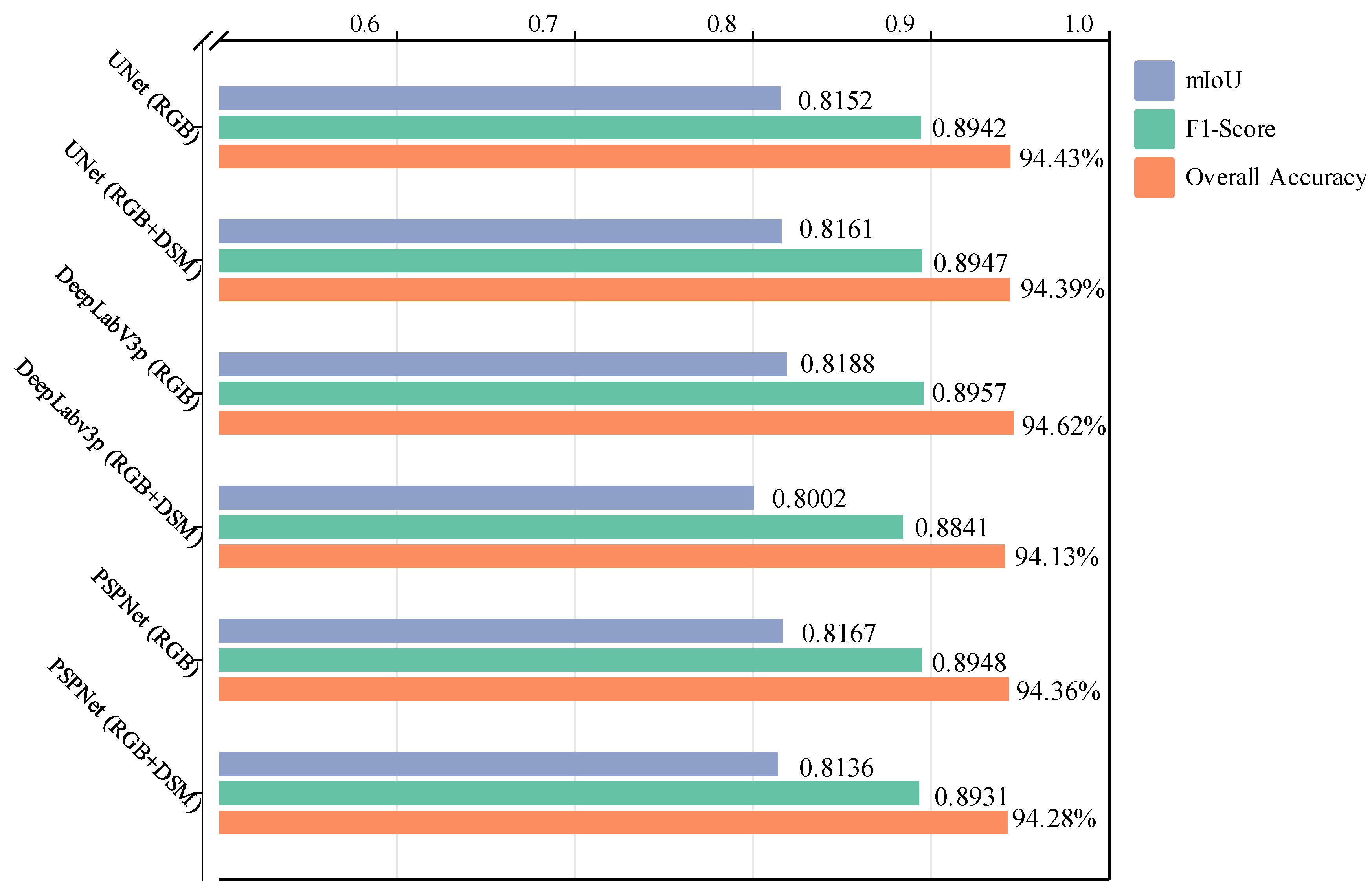
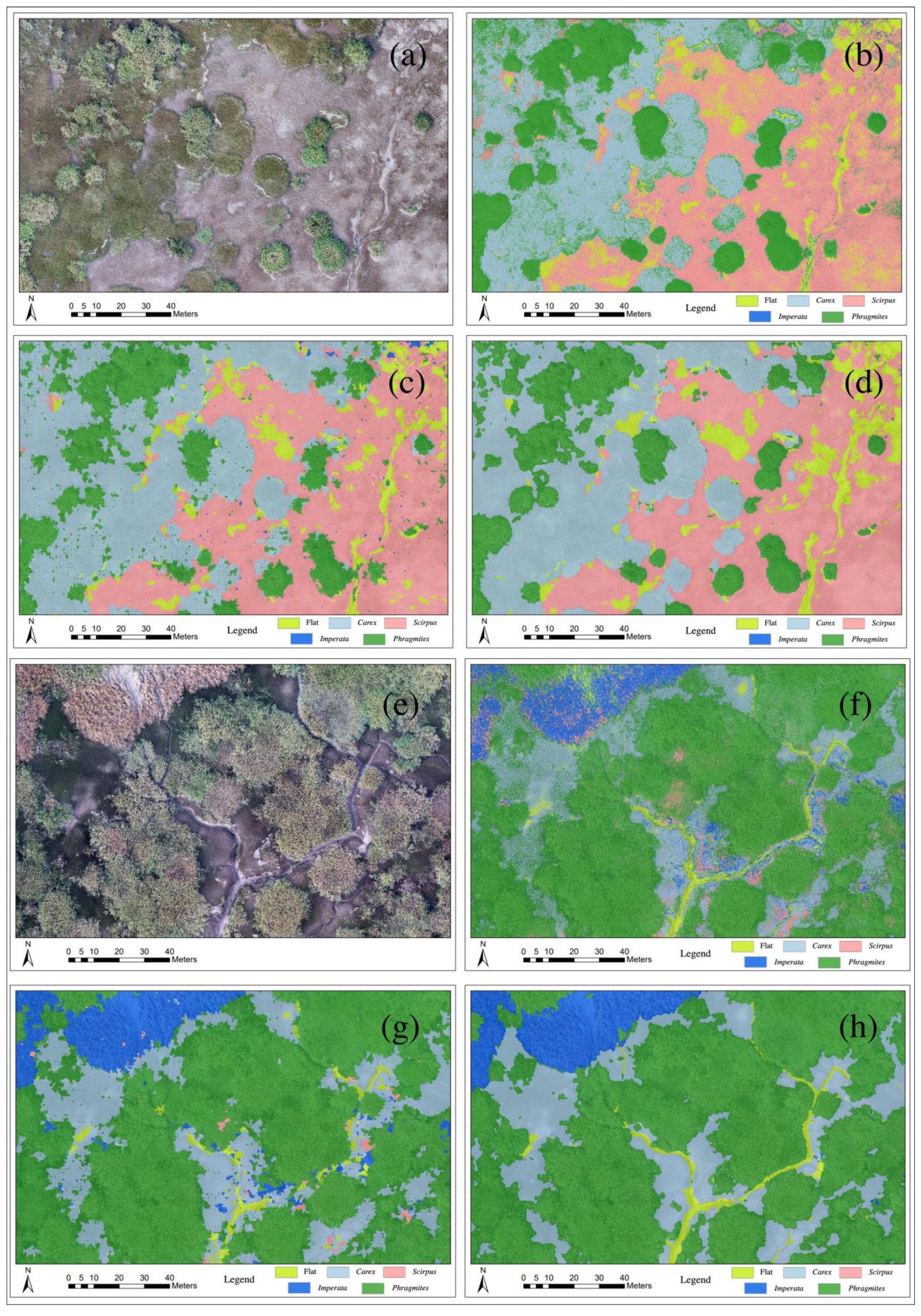
3.4. Results of DL Classification and the Comparison with PB and OBIA
4. Discussion
4.1. UAV Data Processing and Mapping Based on GEE
4.2. PB and OBIA Classification Based on RGB-UAV Data with Feature Engineering
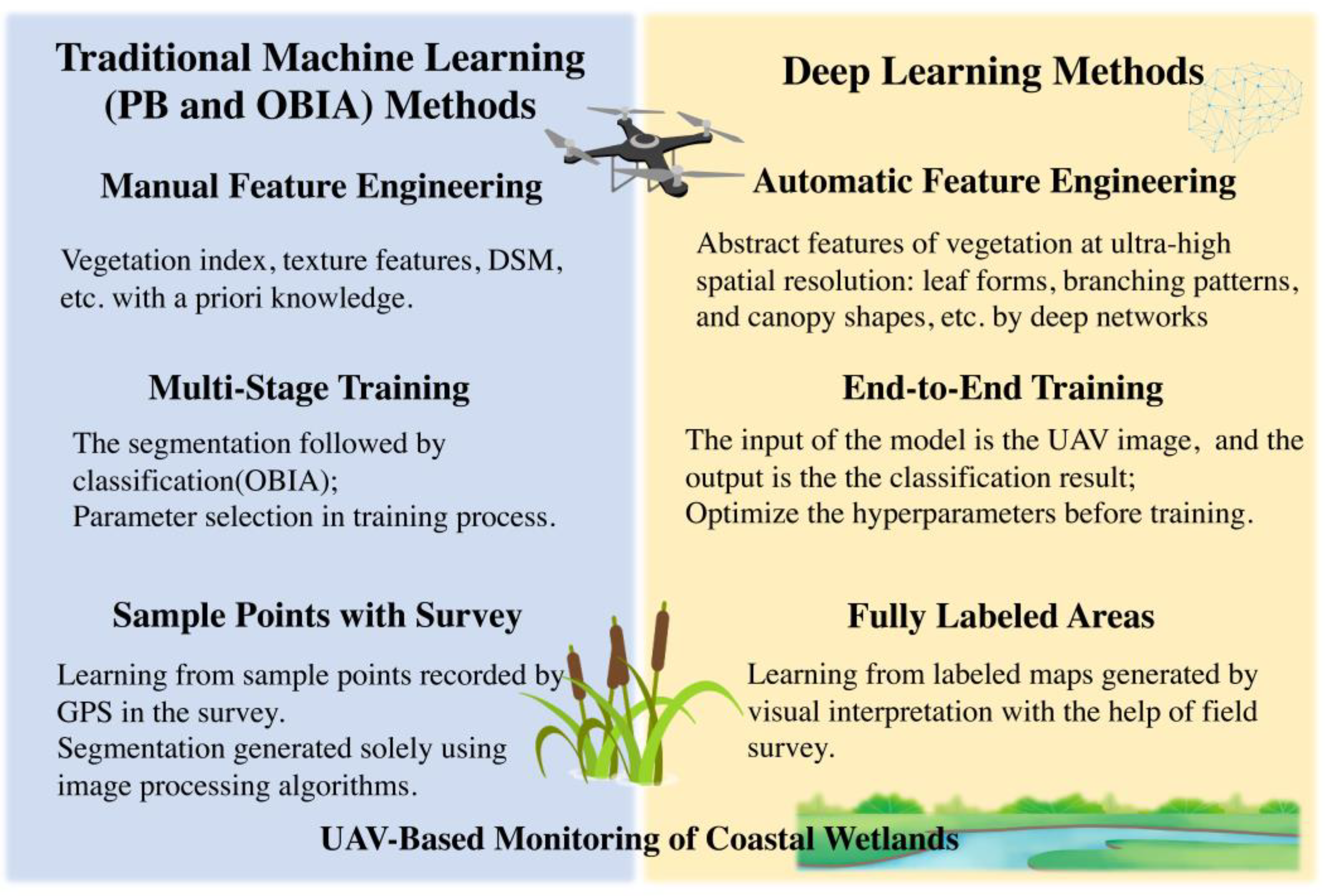
4.3. Paradigm Shift between PB, OBIA, and DL Classification
4.4. Coastal Wetland Monitoring Based on UAV, DL, and Cloud Computing Platform
5. Conclusions
- This study showed the feasibility of using GEE to process ultra-high-resolution UAV data and successfully explored the implementation of the OBIA method for the first time to classify coastal wetland vegetation based on GEE.
- This study once again confirmed that OBIA is better than PB classification in terms of both classification metrics and classification result map, and can reduce the pepper effect.
- Our results revealed that DSM played the most important role in PB and OBIA classifications, whereas the addition of DSM seemed to have little improvement in the accuracy of DL models. Moreover, texture features of Correlation were effectively utilized in OBIA classifications and ranked second in feature contribution. In addition, vegetation indices such as NGBDI and NGBRI also ranked high in contribution to PB and OBIA classifications.
- This study demonstrated that the DL model achieves better classification than OBIA and is more capable of reflecting the realistic distribution of vegetation.
- The paradigm shifts from PB and OBIA to the DL method in terms of feature engineering, training methods, and reference data explained the considerable results achieved by the DL method.
Author Contributions
Funding
Data Availability Statement
Conflicts of Interest
Appendix A


References
- Zedler, J.B.; Kercher, S. Wetland Resources: Status, Trends, Ecosystem Services, and Restorability. Annu. Rev. Environ. Resour. 2005, 30, 39–74. [Google Scholar] [CrossRef]
- Barbier, E.B.; Hacker, S.D.; Kennedy, C.; Koch, E.W.; Stier, A.C.; Silliman, B.R. The Value of Estuarine and Coastal Ecosystem Services. Ecol. Monogr. 2011, 81, 169–193. [Google Scholar] [CrossRef]
- Mitsch, W.J.; Bernal, B.; Nahlik, A.M.; Mander, U.; Zhang, L.; Anderson, C.J.; Jorgensen, S.E.; Brix, H. Wetlands, Carbon, and Climate Change. Landsc. Ecol. 2013, 28, 583–597. [Google Scholar] [CrossRef]
- Worm, B.; Barbier, E.B.; Beaumont, N.; Duffy, J.E.; Folke, C.; Halpern, B.S.; Jackson, J.B.C.; Lotze, H.K.; Micheli, F.; Palumbi, S.R.; et al. Impacts of Biodiversity Loss on Ocean Ecosystem Services. Science 2006, 314, 787–790. [Google Scholar] [CrossRef] [PubMed]
- Halpern, B.S.; Walbridge, S.; Selkoe, K.A.; Kappel, C.V.; Micheli, F.; D’Agrosa, C.; Bruno, J.F.; Casey, K.S.; Ebert, C.; Fox, H.E.; et al. A Global Map of Human Impact on Marine Ecosystems. Science 2008, 319, 948–952. [Google Scholar] [CrossRef]
- Barbier, E.B. Valuing Ecosystem Services for Coastal Wetland Protection and Restoration: Progress and Challenges. Resources 2013, 2, 213–230. [Google Scholar] [CrossRef]
- Johannessen, C.L. Marshes Prograding in Oregon: Aerial Photographs. Science 1964, 146, 1575–1578. [Google Scholar] [CrossRef]
- Ozesmi, S.L.; Bauer, M.E. Satellite Remote Sensing of Wetlands. Wetl. Ecol. Manag. 2002, 10, 381–402. [Google Scholar] [CrossRef]
- Adam, E.; Mutanga, O.; Rugege, D. Multispectral and Hyperspectral Remote Sensing for Identification and Mapping of Wetland Vegetation: A Review. Wetl. Ecol. Manag. 2010, 18, 281–296. [Google Scholar] [CrossRef]
- Guo, M.; Li, J.; Sheng, C.; Xu, J.; Wu, L. A Review of Wetland Remote Sensing. Sensors 2017, 17, 777. [Google Scholar] [CrossRef]
- Kaplan, G.; Avdan, U. Monthly Analysis of Wetlands Dynamics Using Remote Sensing Data. ISPRS Int. J. Geo-Inf. 2018, 7, 411. [Google Scholar] [CrossRef]
- Boon, M.A.; Greenfield, R.; Tesfamichael, S. Wetland Assessment Using Unmanned Aerial Vehicle (UAV) Photogrammetry. ISPRS Int. Arch. Photogramm. Remote Sens. Spat. Inf. Sci. 2016, 41B1, 781–788. [Google Scholar] [CrossRef]
- Dronova, I.; Kislik, C.; Dinh, Z.; Kelly, M. A Review of Unoccupied Aerial Vehicle Use in Wetland Applications: Emerging Opportunities in Approach, Technology, and Data. Drones-Basel 2021, 5, 45. [Google Scholar] [CrossRef]
- Ma, Y.; Zhang, J.; Zhang, J. Analysis of Unmanned Aerial Vehicle (UAV) Hyperspectral Remote Sensing Monitoring Key Technology in Coastal Wetland. In Selected Papers of the Photoelectronic Technology Committee Conferences held November 2015; SPIE: Bellingham, WA, USA, 2016; Volume 9796, pp. 721–729. [Google Scholar]
- Correll, M.D.; Hantson, W.; Hodgman, T.P.; Cline, B.B.; Elphick, C.S.; Gregory Shriver, W.; Tymkiw, E.L.; Olsen, B.J. Fine-Scale Mapping of Coastal Plant Communities in the Northeastern USA. Wetlands 2019, 39, 17–28. [Google Scholar] [CrossRef]
- Durgan, S.D.; Zhang, C.; Duecaster, A.; Fourney, F.; Su, H. Unmanned Aircraft System Photogrammetry for Mapping Diverse Vegetation Species in a Heterogeneous Coastal Wetland. Wetlands 2020, 40, 2621–2633. [Google Scholar] [CrossRef]
- Wan, H.; Wang, Q.; Jiang, D.; Fu, J.; Yang, Y.; Liu, X. Monitoring the Invasion of Spartina Alterniflora Using Very High Resolution Unmanned Aerial Vehicle Imagery in Beihai, Guangxi (China). Sci. World J. 2014, 2014, 638296. [Google Scholar] [CrossRef]
- Samiappan, S.; Turnage, G.; Hathcock, L.; Casagrande, L.; Stinson, P.; Moorhead, R. Using Unmanned Aerial Vehicles for High-Resolution Remote Sensing to Map Invasive Phragmites Australis in Coastal Wetlands. Int. J. Remote Sens. 2017, 38, 2199–2217. [Google Scholar] [CrossRef]
- Doughty, C.L.; Cavanaugh, K.C. Mapping Coastal Wetland Biomass from High Resolution Unmanned Aerial Vehicle (UAV) Imagery. Remote Sens. 2019, 11, 540. [Google Scholar] [CrossRef]
- Tang, Y.-N.; Ma, J.; Xu, J.-X.; Wu, W.-B.; Wang, Y.-C.; Guo, H.-Q. Assessing the Impacts of Tidal Creeks on the Spatial Patterns of Coastal Salt Marsh Vegetation and Its Aboveground Biomass. Remote Sens. 2022, 14, 1839. [Google Scholar] [CrossRef]
- Dale, J.; Burnside, N.G.; Hill-Butler, C.; Berg, M.J.; Strong, C.J.; Burgess, H.M. The Use of Unmanned Aerial Vehicles to Determine Differences in Vegetation Cover: A Tool for Monitoring Coastal Wetland Restoration Schemes. Remote Sens. 2020, 12, 4022. [Google Scholar] [CrossRef]
- Adade, R.; Aibinu, A.M.; Ekumah, B.; Asaana, J. Unmanned Aerial Vehicle (UAV) Applications in Coastal Zone Management—a Review. Env. Monit Assess 2021, 193, 154. [Google Scholar] [CrossRef] [PubMed]
- Blaschke, T. Object Based Image Analysis for Remote Sensing. ISPRS-J. Photogramm. Remote Sens. 2010, 65, 2–16. [Google Scholar] [CrossRef]
- Ouyang, Z.-T.; Zhang, M.-Q.; Xie, X.; Shen, Q.; Guo, H.-Q.; Zhao, B. A Comparison of Pixel-Based and Object-Oriented Approaches to VHR Imagery for Mapping Saltmarsh Plants. Ecol. Inform. 2011, 6, 136–146. [Google Scholar] [CrossRef]
- Dronova, I. Object-Based Image Analysis in Wetland Research: A Review. Remote Sens. 2015, 7, 6380–6413. [Google Scholar] [CrossRef]
- Owers, C.J.; Rogers, K.; Woodroffe, C.D. Identifying Spatial Variability and Complexity in Wetland Vegetation Using an Object-Based Approach. Int. J. Remote Sens. 2016, 37, 4296–4316. [Google Scholar] [CrossRef]
- Martínez Prentice, R.; Villoslada Peciña, M.; Ward, R.D.; Bergamo, T.F.; Joyce, C.B.; Sepp, K. Machine Learning Classification and Accuracy Assessment from High-Resolution Images of Coastal Wetlands. Remote Sens. 2021, 13, 3669. [Google Scholar] [CrossRef]
- Osco, L.P.; Junior, J.M.; Ramos, A.P.M.; Jorge, L.A.d.C.; Fatholahi, S.N.; Silva, J.d.A.; Matsubara, E.T.; Pistori, H.; Gonçalves, W.N.; Li, J. A Review on Deep Learning in UAV Remote Sensing. arXiv 2021, arXiv:2101.10861. [Google Scholar] [CrossRef]
- Long, J.; Shelhamer, E.; Darrell, T. Fully Convolutional Networks for Semantic Segmentation. In Proceedings of the 2015 IEEE Conference on Computer Vision and Pattern Recognition (CVPR), Boston, MA, USA, 7–12 June 2015; IEEE: New York, NY, USA, 2015; pp. 3431–3440, ISBN 978-1-4673-6964-0. [Google Scholar]
- Kattenborn, T.; Eichel, J.; Fassnacht, F.E. Convolutional Neural Networks Enable Efficient, Accurate and Fine-Grained Segmentation of Plant Species and Communities from High-Resolution UAV Imagery. Sci. Rep. 2019, 9, 17656. [Google Scholar] [CrossRef]
- Pashaei, M.; Kamangir, H.; Starek, M.J.; Tissot, P. Review and Evaluation of Deep Learning Architectures for Efficient Land Cover Mapping with UAS Hyper-Spatial Imagery: A Case Study Over a Wetland. Remote Sens. 2020, 12, 959. [Google Scholar] [CrossRef]
- Huang, H.; Lan, Y.; Yang, A.; Zhang, Y.; Wen, S.; Deng, J. Deep Learning versus Object-Based Image Analysis (OBIA) in Weed Mapping of UAV Imagery. Int. J. Remote Sens. 2020, 41, 3446–3479. [Google Scholar] [CrossRef]
- Diez, Y.; Kentsch, S.; Fukuda, M.; Caceres, M.L.L.; Moritake, K.; Cabezas, M. Deep Learning in Forestry Using UAV-Acquired RGB Data: A Practical Review. Remote Sens. 2021, 13, 2837. [Google Scholar] [CrossRef]
- Lam, O.H.Y.; Dogotari, M.; Prüm, M.; Vithlani, H.N.; Roers, C.; Melville, B.; Zimmer, F.; Becker, R. An Open Source Workflow for Weed Mapping in Native Grassland Using Unmanned Aerial Vehicle: Using Rumex Obtusifolius as a Case Study. Eur. J. Remote Sens. 2021, 54, 71–88. [Google Scholar] [CrossRef]
- Bhatnagar, S.; Gill, L.; Ghosh, B. Drone Image Segmentation Using Machine and Deep Learning for Mapping Raised Bog Vegetation Communities. Remote Sens. 2020, 12, 2602. [Google Scholar] [CrossRef]
- Gonzalez-Perez, A.; Abd-Elrahman, A.; Wilkinson, B.; Johnson, D.J.; Carthy, R.R. Deep and Machine Learning Image Classification of Coastal Wetlands Using Unpiloted Aircraft System Multispectral Images and Lidar Datasets. Remote Sens. 2022, 14, 3937. [Google Scholar] [CrossRef]
- Morgan, G.R.; Hodgson, M.E.; Wang, C.; Schill, S.R. Unmanned Aerial Remote Sensing of Coastal Vegetation: A Review. Ann. GIS 2022, 28, 385–399. [Google Scholar] [CrossRef]
- Zhou, H.; Fu, L.; Sharma, R.P.; Lei, Y.; Guo, J. A Hybrid Approach of Combining Random Forest with Texture Analysis and VDVI for Desert Vegetation Mapping Based on UAV RGB Data. Remote Sens. 2021, 13, 1891. [Google Scholar] [CrossRef]
- Zhou, R.; Yang, C.; Li, E.; Cai, X.; Yang, J.; Xia, Y. Object-Based Wetland Vegetation Classification Using Multi-Feature Selection of Unoccupied Aerial Vehicle RGB Imagery. Remote Sens. 2021, 13, 4910. [Google Scholar] [CrossRef]
- Gorelick, N.; Hancher, M.; Dixon, M.; Ilyushchenko, S.; Thau, D.; Moore, R. Google Earth Engine: Planetary-Scale Geospatial Analysis for Everyone. Remote Sens. Environ. 2017, 202, 18–27. [Google Scholar] [CrossRef]
- Lukacz, P.M. Data Capitalism, Microsoft’s Planetary Computer, and the Biodiversity Informatics Community. In Information for a Better World: Shaping the Global Future; Smits, M., Ed.; Springer International Publishing: Cham, Switzerland, 2022; pp. 355–369. [Google Scholar]
- Bennett, M.K.; Younes, N.; Joyce, K. Automating Drone Image Processing to Map Coral Reef Substrates Using Google Earth Engine. Drones 2020, 4, 50. [Google Scholar] [CrossRef]
- Tamiminia, H.; Salehi, B.; Mahdianpari, M.; Quackenbush, L.; Adeli, S.; Brisco, B. Google Earth Engine for Geo-Big Data Applications: A Meta-Analysis and Systematic Review. ISPRS J. Photogramm. Remote Sens. 2020, 164, 152–170. [Google Scholar] [CrossRef]
- Tassi, A.; Vizzari, M. Object-Oriented LULC Classification in Google Earth Engine Combining SNIC, GLCM, and Machine Learning Algorithms. Remote Sens. 2020, 12, 3776. [Google Scholar] [CrossRef]
- Ma, Z.; Li, B.; Jing, K.; Zhao, B.; Tang, S.; Chen, J. Effects of Tidewater on the Feeding Ecology of Hooded Crane (Grus Monacha) and Conservation of Their Wintering Habitats at Chongming Dongtan, China. Ecol. Res. 2003, 18, 321–329. [Google Scholar] [CrossRef]
- Corti Meneses, N.; Brunner, F.; Baier, S.; Geist, J.; Schneider, T. Quantification of Extent, Density, and Status of Aquatic Reed Beds Using Point Clouds Derived from UAV–RGB Imagery. Remote Sens. 2018, 10, 1869. [Google Scholar] [CrossRef]
- Morgan, G.R.; Wang, C.; Morris, J.T. RGB Indices and Canopy Height Modelling for Mapping Tidal Marsh Biomass from a Small Unmanned Aerial System. Remote Sens. 2021, 13, 3406. [Google Scholar] [CrossRef]
- Woebbecke, D.M.; Meyer, G.E.; Bargen, K.V.; Mortensen, D.A. Color Indices for Weed Identification Under Various Soil, Residue, and Lighting Conditions. Trans. ASAE 1995, 38, 259–269. [Google Scholar] [CrossRef]
- Torres-Sánchez, J.; Peña, J.M.; de Castro, A.I.; López-Granados, F. Multi-Temporal Mapping of the Vegetation Fraction in Early-Season Wheat Fields Using Images from UAV. Comput. Electron. Agric. 2014, 103, 104–113. [Google Scholar] [CrossRef]
- Du, M.; Noguchi, N. Monitoring of Wheat Growth Status and Mapping of Wheat Yield’s within-Field Spatial Variations Using Color Images Acquired from UAV-Camera System. Remote Sens. 2017, 9, 289. [Google Scholar] [CrossRef]
- Sonnentag, O.; Hufkens, K.; Teshera-Sterne, C.; Young, A.M.; Friedl, M.; Braswell, B.H.; Milliman, T.; O’Keefe, J.; Richardson, A.D. Digital Repeat Photography for Phenological Research in Forest Ecosystems. Agric. For. Meteorol. 2012, 152, 159–177. [Google Scholar] [CrossRef]
- XiaoQin, W.; MiaoMiao, W.; ShaoQiang, W.; YunDong, W. Extraction of vegetation information from visible unmanned aerial vehicle images. Trans. Chin. Soc. Agric. Eng. 2015, 31, 152–159. [Google Scholar]
- Reed, B.; Brown, J.; Vanderzee, D.; Loveland, T.; Merchant, J.; Ohlen, D. Measuring Phenological Variability from Satellite Imagery. J. Veg. Sci. 1994, 5, 703–714. [Google Scholar] [CrossRef]
- Achanta, R.; Süsstrunk, S. Superpixels and Polygons Using Simple Non-Iterative Clustering. In Proceedings of the 2017 IEEE Conference on Computer Vision and Pattern Recognition (CVPR), Honolulu, HI, USA, 21–26 July 2017; pp. 4895–4904. [Google Scholar]
- Mahdianpari, M.; Salehi, B.; Mohammadimanesh, F.; Homayouni, S.; Gill, E. The First Wetland Inventory Map of Newfoundland at a Spatial Resolution of 10 m Using Sentinel-1 and Sentinel-2 Data on the Google Earth Engine Cloud Computing Platform. Remote Sens. 2019, 11, 43. [Google Scholar] [CrossRef]
- Vizzari, M. PlanetScope, Sentinel-2, and Sentinel-1 Data Integration for Object-Based Land Cover Classification in Google Earth Engine. Remote Sens. 2022, 14, 2628. [Google Scholar] [CrossRef]
- Sheykhmousa, M.; Mahdianpari, M.; Ghanbari, H.; Mohammadimanesh, F.; Ghamisi, P.; Homayouni, S. Support Vector Machine Versus Random Forest for Remote Sensing Image Classification: A Meta-Analysis and Systematic Review. IEEE J. Sel. Top. Appl. Earth Obs. Remote Sens. 2020, 13, 6308–6325. [Google Scholar] [CrossRef]
- Amani, M.; Ghorbanian, A.; Ahmadi, S.A.; Kakooei, M.; Moghimi, A.; Mirmazloumi, S.M.; Moghaddam, S.H.A.; Mahdavi, S.; Ghahremanloo, M.; Parsian, S.; et al. Google Earth Engine Cloud Computing Platform for Remote Sensing Big Data Applications: A Comprehensive Review. IEEE J. Sel. Top. Appl. Earth Obs. Remote Sens. 2020, 13, 5326–5350. [Google Scholar] [CrossRef]
- Belgiu, M.; Drăguţ, L. Random Forest in Remote Sensing: A Review of Applications and Future Directions. ISPRS J. Photogramm. Remote Sens. 2016, 114, 24–31. [Google Scholar] [CrossRef]
- Zhang, X.; Han, L.; Han, L.; Zhu, L. How Well Do Deep Learning-Based Methods for Land Cover Classification and Object Detection Perform on High Resolution Remote Sensing Imagery? Remote Sens. 2020, 12, 1–29. [Google Scholar] [CrossRef]
- Wu, Q. Geemap: A Python Package for Interactive Mapping with Google Earth Engine. J. Open Source Softw. 2020, 5, 2305. [Google Scholar] [CrossRef]
- Ronneberger, O.; Fischer, P.; Brox, T. U-Net: Convolutional Networks for Biomedical Image Segmentation. In Medical Image Computing and Computer-Assisted Intervention—MICCAI 2015; Springer: Cham, Switzerland, 2015. [Google Scholar]
- Zhao, H.; Shi, J.; Qi, X.; Wang, X.; Jia, J. Pyramid Scene Parsing Network. In Proceedings of the 30th IEEE Conference on Computer Vision and Pattern Recognition (CVPR 2017), Honolulu, HI, USA, 21–26 July 2017; IEEE: New York, NY, USA, 2017; pp. 6230–6239, ISBN 978-1-5386-0457-1. [Google Scholar]
- Chen, L.-C.; Papandreou, G.; Schroff, F.; Adam, H. Rethinking Atrous Convolution for Semantic Image Segmentation. arXiv 2017, arXiv:1706.05587. [Google Scholar]
- Paszke, A.; Gross, S.; Massa, F.; Lerer, A.; Bradbury, J.; Chanan, G.; Killeen, T.; Lin, Z.; Gimelshein, N.; Antiga, L.; et al. PyTorch: An Imperative Style, High-Performance Deep Learning Library. In Advances in Neural Information Processing Systems 32 (NeurIPS 2019); Wallach, H., Larochelle, H., Beygelzimer, A., d’Alche-Buc, F., Fox, E., Garnett, R., Eds.; Neural Information Processing Systems (NeurIPS): La Jolla, CA, USA, 2019; Volume 32. [Google Scholar]
- Goutte, C.; Gaussier, E. A Probabilistic Interpretation of Precision, Recall and F-Score, with Implication for Evaluation. In Advances in Information Retrieval; Losada, D.E., Fernández-Luna, J.M., Eds.; Springer: Berlin/Heidelberg, Germany, 2005; pp. 345–359. [Google Scholar]
- Hoeser, T.; Kuenzer, C. Object Detection and Image Segmentation with Deep Learning on Earth Observation Data: A Review-Part I: Evolution and Recent Trends. Remote Sens. 2020, 12, 1667. [Google Scholar] [CrossRef]
- Ward, R.D.; Burnside, N.G.; Joyce, C.B.; Sepp, K. Importance of Microtopography in Determining Plant Community Distribution in Baltic Coastal Wetlands. J. Coast. Res. 2016, 32, 1062–1070. [Google Scholar] [CrossRef]
- Yuan, H.; Liu, Z.; Cai, Y.; Zhao, B. Research on Vegetation Information Extraction from Visible UAV Remote Sensing Images. In Proceedings of the 2018 Fifth International Workshop on Earth Observation and Remote Sensing Applications (EORSA), Xi’an, China, 18–20 June 2018; pp. 1–5. [Google Scholar]
- Villoslada, M.; Bergamo, T.F.; Ward, R.D.; Burnside, N.G.; Joyce, C.B.; Bunce, R.G.H.; Sepp, K. Fine Scale Plant Community Assessment in Coastal Meadows Using UAV Based Multispectral Data. Ecol. Indic. 2020, 111, 105979. [Google Scholar] [CrossRef]
- Du, B.; Mao, D.; Wang, Z.; Qiu, Z.; Yan, H.; Feng, K.; Zhang, Z. Mapping Wetland Plant Communities Using Unmanned Aerial Vehicle Hyperspectral Imagery by Comparing Object/Pixel-Based Classifications Combining Multiple Machine-Learning Algorithms. IEEE J. Sel. Top. Appl. Earth Obs. Remote Sens. 2021, 14, 8249–8258. [Google Scholar] [CrossRef]
- Pande-Chhetri, R.; Abd-Elrahman, A.; Liu, T.; Morton, J.; Wilhelm, V.L. Object-Based Classification of Wetland Vegetation Using Very High-Resolution Unmanned Air System Imagery. Eur. J. Remote Sens. 2017, 50, 564–576. [Google Scholar] [CrossRef]
- Rezaee, M.; Mahdianpari, M.; Zhang, Y.; Salehi, B. Deep Convolutional Neural Network for Complex Wetland Classification Using Optical Remote Sensing Imagery. IEEE J. Sel. Top. Appl. Earth Obs. Remote Sens. 2018, 11, 3030–3039. [Google Scholar] [CrossRef]
- Kattenborn, T.; Leitloff, J.; Schiefer, F.; Hinz, S. Review on Convolutional Neural Networks (CNN) in Vegetation Remote Sensing. ISPRS J. Photogramm. Remote Sens. 2021, 173, 24–49. [Google Scholar] [CrossRef]
- Yang, L.; Driscol, J.; Sarigai, S.; Wu, Q.; Chen, H.; Lippitt, C.D. Google Earth Engine and Artificial Intelligence (AI): A Comprehensive Review. Remote Sens. 2022, 14, 3253. [Google Scholar] [CrossRef]
- Liu, T.; Abd-Elrahman, A. Deep Convolutional Neural Network Training Enrichment Using Multi-View Object-Based Analysis of Unmanned Aerial Systems Imagery for Wetlands Classification. ISPRS-J. Photogramm. Remote Sens. 2018, 139, 154–170. [Google Scholar] [CrossRef]


| Train & Validation Set in DL | Test Set in DL | ML (by Random Sampling) | ||||
|---|---|---|---|---|---|---|
| Class | Labelled Pixels | Percentage | Labelled Pixels | Percentage | Labelled Pixels (Sum) | Percentage |
| Flat | 11,799,975 | 10.55% | 9,993,984 | 9.82% | 21,793,959 | 10.20% |
| Imperata cylindrica | 10,488,110 | 9.38% | 10,488,110 | 10.31% | 20,976,220 | 9.82% |
| Phragmites trails | 65,549,739 | 58.61% | 56,959,595 | 55.97% | 122,509,334 | 57.35% |
| Carex scabrifolia Steud | 14,713,632 | 13.16% | 17,406,834 | 17.10% | 32,120,466 | 15.04% |
| Scripus mariqueter | 9,287,021 | 8.30% | 6,916,704 | 6.80% | 16,203,725 | 7.59% |
| Total | 111,838,477 | 100.00% | 101,765,227 | 100.00% | 213,603,704 | 100.00% |
| Vegetation Indices | Formulation | References |
|---|---|---|
| ExGI | [48] | |
| NGRDI | [49] | |
| NGBDI | [50] | |
| GCC | [51] | |
| VDVI | [38,52] |
| Features Name | Description |
|---|---|
| GLCM_asm | Angular Second Moment; measures the number of repeated pairs |
| GLCM_contrast | Contrast; measures the local contrast of an image |
| GLCM_corr | Correlation; measures the correlation between pairs of pixels |
| GLCM_var | Variance; measures how spread out the distribution of gray-levels is |
| GLCM_idm | Inverse Difference Moment; measures the homogeneity |
| GLCM_savg | Sum Average; measures the mean of the gray level sum distribution of the image |
| GLCM_ent | Entropy; measures the degree of the disorder among pixels in the image |
| Classification Paradigm | Classification Model | Combination of Features |
|---|---|---|
| PB and OBIA | Random Forest | RGB |
| PB and OBIA | Random Forest | RGB + DSM |
| PB and OBIA | Random Forest | RGB + VI |
| PB and OBIA | Random Forest | RGB + Texture |
| PB and OBIA | Random Forest | RGB + VI + Texture |
| PB and OBIA | Random Forest | RGB + VI + Texture + DSM |
| DL | U-Net | RGB RGB + DSM |
| DL | DeepLabV3+ | RGB RGB + DSM |
| DL | PSPNet | RGB RGB + DSM |
| Class | PB (Full Feature) | OBIA (Full Feature) | DL (RGB) | ||||||
|---|---|---|---|---|---|---|---|---|---|
| Precision | Recall | IoU | Precision | Recall | IoU | Precision | Recall | IoU | |
| Flat | 0.7929 | 0.7258 | 0.4056 | 0.8401 | 0.8126 | 0.5366 | 0.7478 | 0.7670 | 0.6093 |
| Imperata cylindrica | 0.6938 | 0.5483 | 0.4636 | 0.8163 | 0.7293 | 0.6741 | 0.9532 | 0.9074 | 0.8687 |
| Phragmites trails | 0.8560 | 0.8884 | 0.8346 | 0.9065 | 0.9202 | 0.8783 | 0.9699 | 0.9832 | 0.9541 |
| Carex scabrifolia Steud | 0.7953 | 0.7663 | 0.5162 | 0.8642 | 0.8654 | 0.6500 | 0.9453 | 0.8933 | 0.8494 |
| Scripusmariqueter | 0.7832 | 0.8286 | 0.5460 | 0.8774 | 0.8859 | 0.7129 | 0.8874 | 0.9057 | 0.8123 |
| Overall accuracy (%) | 81.47% | 87.98% | 94.62% | ||||||
| F1-Score | 0.7675 | 0.8517 | 0.8957 | ||||||
| mIoU | 0.5532 | 0.6904 | 0.8188 | ||||||
Publisher’s Note: MDPI stays neutral with regard to jurisdictional claims in published maps and institutional affiliations. |
© 2022 by the authors. Licensee MDPI, Basel, Switzerland. This article is an open access article distributed under the terms and conditions of the Creative Commons Attribution (CC BY) license (https://creativecommons.org/licenses/by/4.0/).
Share and Cite
Zheng, J.-Y.; Hao, Y.-Y.; Wang, Y.-C.; Zhou, S.-Q.; Wu, W.-B.; Yuan, Q.; Gao, Y.; Guo, H.-Q.; Cai, X.-X.; Zhao, B. Coastal Wetland Vegetation Classification Using Pixel-Based, Object-Based and Deep Learning Methods Based on RGB-UAV. Land 2022, 11, 2039. https://doi.org/10.3390/land11112039
Zheng J-Y, Hao Y-Y, Wang Y-C, Zhou S-Q, Wu W-B, Yuan Q, Gao Y, Guo H-Q, Cai X-X, Zhao B. Coastal Wetland Vegetation Classification Using Pixel-Based, Object-Based and Deep Learning Methods Based on RGB-UAV. Land. 2022; 11(11):2039. https://doi.org/10.3390/land11112039
Chicago/Turabian StyleZheng, Jun-Yi, Ying-Ying Hao, Yuan-Chen Wang, Si-Qi Zhou, Wan-Ben Wu, Qi Yuan, Yu Gao, Hai-Qiang Guo, Xing-Xing Cai, and Bin Zhao. 2022. "Coastal Wetland Vegetation Classification Using Pixel-Based, Object-Based and Deep Learning Methods Based on RGB-UAV" Land 11, no. 11: 2039. https://doi.org/10.3390/land11112039
APA StyleZheng, J.-Y., Hao, Y.-Y., Wang, Y.-C., Zhou, S.-Q., Wu, W.-B., Yuan, Q., Gao, Y., Guo, H.-Q., Cai, X.-X., & Zhao, B. (2022). Coastal Wetland Vegetation Classification Using Pixel-Based, Object-Based and Deep Learning Methods Based on RGB-UAV. Land, 11(11), 2039. https://doi.org/10.3390/land11112039