Article

Morphological Characteristics and Hydrological Connectivity Evaluation of Tidal Creeks in Coastal Wetlands

1
College of Ocean Science and Environment, Dalian Ocean University, Dalian 116023, China
2
Technology Innovation Center for Coastal Ecological Environment and Disaster Protection, Dalian 116023, China
3
National Marine Environmental Monitoring Center, Dalian 116023, China
*
Authors to whom correspondence should be addressed.
Land 2022, 11(10), 1707; https://doi.org/10.3390/land11101707
Submission received: 16 September 2022 / Revised: 27 September 2022 / Accepted: 29 September 2022 / Published: 1 October 2022
(This article belongs to the Special Issue Monitoring and Simulation of Wetland Ecological Processes)

Abstract

:
Tidal creeks play a critical role in delivering water, suspended sediments, and nutrients to coastal wetlands, so it is important to understand the characteristics of the tidal creek system to guide the development and sustainable utilization of coastal wetlands. Using the coastal wetlands of the Liao River Estuary (LRE) as a study area, this study accurately divided the tidal flat based on the principle of tidal correction, extracted the linear features of tidal creeks using high-resolution remote sensing (RS) data, and then classified the tidal creeks on a tidal flat using the tidal creek ordering algorithm. Our study aimed to quantify the morphological characteristics of tidal creeks and qualitatively evaluate the parameters of the tidal creek network in the study area. The study results show obvious spatial heterogeneity in the order and the average length of tidal creeks in the coastal wetlands of the LRE. With the increase in the order of tidal creeks, the average length of tidal creeks increased exponentially and the number of tidal creeks decreased exponentially in the study area. The total density of tidal creeks was related to the beach surface elevation gradient, and the density and frequency of tidal creeks reduced substantially with an increase in the order of tidal creeks. The sinuosity ratio of tidal creeks declined sharply with a fall in the beach surface elevation gradient. The average bifurcation ratio of tidal creeks in the upper intertidal zone was higher than that in other zones, indicating that the tidal creeks in the upper intertidal zone were erratic. In addition, the hydrological connectivity of the tidal creek network in the upper intertidal zone and the development of the tidal creek system in the supratidal zone were the highest in the LRE. The study results help understand the spatial variations in tidal creek morphology under the influence of tidal hydrodynamics.

1. Introduction

As the most vulnerable and economically important ecosystem in the world, coastal wetlands can provide sufficient nutrients and organic matter for marine animals and salt marsh plants living on a tidal flat, also playing a crucial role in ecological protection, biodiversity maintenance, flood prevention, and water purification [1,2,3]. One of the most active micro-geomorphology units of the tidal flat, tidal creeks are widely distributed in the coastal wetlands and connect to a bay or an estuary to transport nutrients, deliver sediments, and help in vegetation colonization and diffusion [4,5]. As a transmission medium, tidal creeks can effectively promote the diffusion of salt marsh vegetation seeds and the saline and freshwater interactions within the tidal creek network regulate the spatial distribution and survival rate of salt marsh plants [6]. The morphological characteristics of tidal creeks are obviously different under the influence of hydrodynamics and anthropogenic activities [7]. Vijay et al. [8] revealed that the creek width was reduced due to urbanization. Park et al. [9] demonstrated that the length, number and direction of tidal creeks changed obviously over the period of a reclamation project. Commonly, the tidal hydrodynamics of tidal creeks lead to channel migration, headward erosion, and siltation, which can destabilize a tidal flat [10,11]; the spatial morphology of tidal creeks changes frequently with the increase in tidal hydrodynamics [12]. The spatial variation in tidal creeks on a tidal flat helps better understand the development mechanism of tidal creeks, and the related data can be applied to managing coastal wetlands.
A key challenge in studying the spatial variation in tidal creeks is to extract their linear features over a large region. In recent years, RS technology has shown to be an effective tool for extracting these data [13,14]. There are three methods for extracting the tidal creek system based on RS technology: the automatic method, the semi-automatic method, and visual interpretation. In the automatic method, the eight-direction flow accumulation model [15] or the thresholding method [16] is used to extract the tidal creek network from a digital elevation model or high-resolution airborne LiDAR [17,18]. This method can be effective when the surface elevation gradients in the study areas are steep [19]. The visual interpretation method has high precision in extracting the linear features of narrow tidal creeks, but it is time consuming and laborious, making it unsuitable for extracting tidal creek networks in large coastal wetlands [20]. The semi-automatic method, combining automatic technology with visual interpretation, is widely used to extract linear features of tidal creeks from RS images [21]. For example, Eom et al. [22] extracted linear features of tidal creeks from remote sensing imagery of the tidal flat of Geunso Bay, Korea, using a semi-automatic method of image enhancement and visual interpretation.
Quantitative analysis of the morphological characteristics of tidal creeks may help understand the intensity of tidal hydrodynamics and evaluate the evolution patterns of tidal creeks on tidal flats. Traditionally, methods, such as field investigation [23,24] and hydrological experiments [25,26] have been used to measure the morphological characteristics of tidal creeks. However, it is difficult to obtain the morphological characteristics of tidal creeks in large coastal wetlands via field investigation. The hydrological experiment method uses a small-scale laboratory to investigate the morphology process in a tidal creek system but cannot identify the evolution patterns of tidal creeks under a complex hydrodynamic environment. With the development of RS technology, high-resolution RS images may help understand the spatial variations in tidal creek morphology on a tidal flat. For instance, Xie et al. [12] explored the spatial–temporal changes in the tidal creek morphology of the Yellow River Delta under a long time series. Zhao et al. [27] quantitatively analyzed the spatial morphological differences in tidal creeks along the central coast of Jiangsu, China. Previous studies have tended to focus on extracting the morphological characteristics of tidal creeks, including the order [28], the length [29], the width [30,31], the density [13], and the sinuosity ratio [32]. However, relatively fewer studies have been conducted to analyze the fractal dimension and connectivity of tidal creeks, which reflect the complexity and the hydrological connectivity of the tidal creek system, respectively.
The coastal wetlands with high hydrological connectivity are an important habitat for marine animals and salt marshes [33,34]. Since the tidal creek network is remarkably similar to the river channel network, some studies have introduced the characteristic indexes of network circuitry (α), the edge–node ratio (β), and network connectivity (γ) to assess the structural connectivity of the tidal creek network in the coastal wetlands of river deltas [35]. For example, Yu et al. [5] quantitatively analyzed the spatial–temporal changes in the connectivity indexes of the tidal creek network of the Yellow River Estuary. Feng et al. [36] calculated the hydrological connectivity of different zones on the basis of the hydraulic resistance and graph theory and showed that the hydrological connectivity of the tidal flat was significantly increased in regions where the main streams of the Yellow River and tidal creeks were concentrated. The parameters of a tidal creek network are important for monitoring the hydrological connectivity of tidal zones and making decisions for protecting tidal flat resources.
As one of the ecologically important estuaries in China, the LRE is formed by the sedimentation of four rivers flowing into Liaodong Bay. Since the LRE is a tide-dominated estuary, tidal hydrodynamic differences on the tidal flats result in spatial variations in the tidal creek morphology. However, there are few quantitative studies on these variations. The objectives of this study were to: (1) use the tidal creek ordering algorithm to classify tidal creeks from high-resolution RS imagery of the coastal wetlands of the LRE, (2) calculate the six morphological parameters of tidal creeks and two sets of parameters of tidal creek network properties, and (3) quantitatively analyze the morphological characteristics of tidal creeks and qualitatively evaluate the complexity and hydrological connectivity of the tidal creek network on the overall and zonal scale.

2. Materials and Methods

2.1. Study Area

The coastal wetland of the LRE (40°43′54″~40°57′13″ N, 121°31′55″~121°57′0″ E) lies in the north of Liaodong Bay, located in the northernmost estuary wetland of China (Figure 1). This area represents a typical coastal ecosystem that is influenced by freshwater influx from the Liao River, the Daliao River, the Daling River, and the Xiaoling River, as well as saline water influx from Liaodong Bay [37]. Tides adjacent to this tidal wetland are semi-diurnal, with two high tides and two low tides each day. The mean tidal range is 2.7 m, and the maximum tidal range is 4 m. The salt marshes of Suaeda salsa (S. salsa) and Phragmites australis (P. autralis) grow on the tidal flats, presenting rare landscapes of “red beaches” and “green carpets” in the summer and autumn [38].

2.2. Datasets

The complex environmental conditions in coastal wetlands do not allow traditional field surveys. With the development of the RS technology, it has been widely used to map wetland vegetation types and detect historical changes in ecosystem cover, as well as investigate the wetland degradation status. The Landsat 8 Operational Land Imager (OLI) images used in this study were downloaded from the Chinese Academy of Sciences (http://www.gscloud.cn, accessed on 10 January 2022). The spatial resolution of the images was 30 m and orbit number 120/32. Guided by the tide table for Laobeihe, our study selected images in low-tide periods on 29 May 2021 and 20 October 2021 for the tidal flat zonation. Moreover, to extract the linear features of tidal creeks in the LRE, our study collected Jilin1-KF01A images from 14 August 2021 and 13 November 2021. The images by the Jilin1-KF01A commercial satellite, constructed and managed by Chang Guang Satellite Technology Co., Ltd., Changchun, China (CGSTL), had a higher spatial resolution, of 0.8 m [39]. The initial Landsat-8 OLI and Jilin1-KF01A images were an L1T standard data product and underwent radiation correction, geometric correction, and terrain correction. Subsequent RS images were pre-processed via radiometric calibration and atmospheric correction.

2.3. Methods

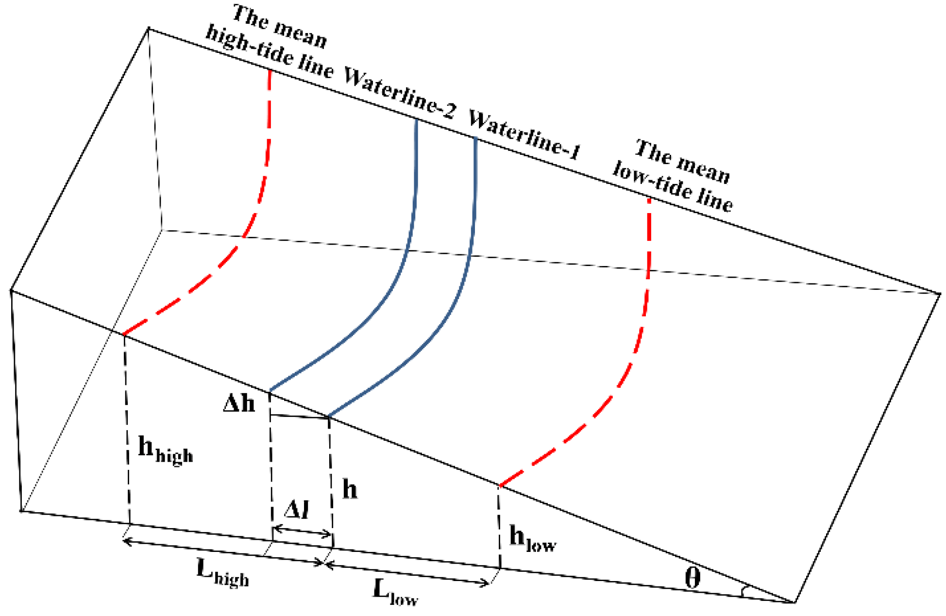
2.3.1. The Instantaneous Waterline Extraction

A silt coast is a large silt–muddy beach created by the action of river sedimentation and seawater erosion. In the LRE, the tidal flat is a typical mudflat with a gentle slope, and the coastline is indistinguishable because of the mixing of water and suspended sediments [40]. To use the instantaneous waterline for the accurate zonation of tidal flats, our study displayed a false color image by using the 5, 4, and 3 bands of Landsat-8 OLI images, which can significantly distinguish the objects of water, a tidal flat, and vegetation (Figure 2a). In the false color image, the red, dark-green, black, and bright-green areas represent vegetation, tidal flat, aquaculture pond, and water, respectively. To classify the water and land, a maximum likelihood classification method combined with a visual interpretation was conducted according to the color differences of the objects (Figure 2b), and then classical Canny edge detection was used to extract the instantaneous waterline in the study area. The mudflat waterline extracted by the algorithm is consistent with the original image. Thus, our study successfully extracted the instantaneous waterline of the silt–muddy beach in the LRE [41].

2.3.2. Tidal Flat Zonation

The morphological characteristics of tidal creeks in each tidal zone may differ due to the difference in hydrodynamic intensities and sedimentation in these regions. Therefore, the accurate zonation of tidal flats is important for the morphological study of tidal creeks. Previous studies have been carried out on the zonation of tidal flats using sediment characteristics [42], biological distribution [43], and spectral reflectance [28] but relied on subjective inferences. Therefore, our study further improved the zonation method of a tidal flat on the basis of the principle of tidal correction [44], as shown in Figure 3. The specific steps of tidal correction in the coastal wetlands of the LRE are as follows: (1) our study calculated the tidal information at the scene center time of the RS images using the tide gauge data (see Table 1); the tide levels (h) of RS images received on 29 May 2021 and 20 October 2021 were 1.449 m and 1.265 m, respectively and the tide level difference (Δh) between the two images was 0.185 m. (2) The shoreline of the study area was divided into three sections due to the intricate terrains of the coastal wetlands in the LRE, as shown in Figure 4. Our study selected the instantaneous waterline (29 May 2021) as the baseline of the tide correction model, set the vertical line from the baseline to another instantaneous waterline every 300 m as the division line, and then calculated the average length of the division line in each shoreline to obtain the distance of two instantaneous waterlines in the same region (Δl). (3) Our study calculated the slope of each shoreline (θ) and the correction distance of the high tide (Lhigh) and the low tide (Llow) using Equations (1) and (2). Our study obtained the positions of theoretical high tide and low tide by constructing buffer zones based on the correction distance and then conducted a field investigation to assist in the zonation of the tidal flat.
The formulas for calculating these parameters are as follows:
h = H l o w + Δ H 2 [ 1 cos ( T l o w t T l o w T h i g h ) × 180 ° ]
θ = arctan Δ h Δ l
L h i g h = h h i g h h tan θ
L l o w = h h l o w tan θ
where h is the tidal level at the scene center time, θ is the slope of each shoreline, Lhigh is the correction distance of the high tide, Llow is the correction distance of the low tide, Hlow stands for the low tide data of the day, ΔH is the tide range of the day, t is the scene center time of the RS images, Tlow is the time of low tide that same day when Thigh is the time of high tide, Δh is the tidal level difference between two images at the scene center time, Δl is the instantaneous waterline distance between two images at the scene center time, and hhigh refers to the mean high tide data that same year when hlow stands for the mean low tide data.

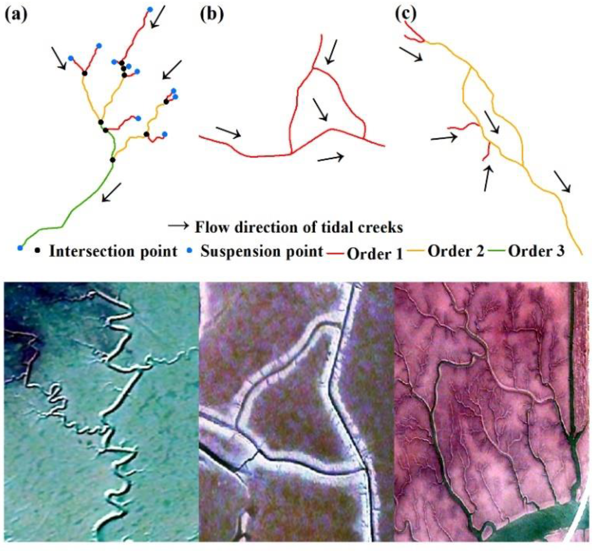
2.3.3. Tidal Creek Extraction

To analyze the morphological characteristics of tidal creeks, our study adopted the semi-automatic method to extract the linear features of tidal creeks on the basis of the high-resolution RS imagery of Jilin1-KF01A. The detailed steps of the method are as follows: (1) To enhance the linear features of narrow tidal creeks, a convolution combined with a noise reduction was used. (2) To extract the linear features of tidal creeks from high-resolution imagery, an object-based support vector machine was applied. (3) To correct and improve the accuracy of tidal creek extraction, manual intervention and post-processing techniques were used. In this study, the tidal creek extraction accuracy was verified by referring to the Google Earth images in the adjacent period combined with a field survey, and the overall extraction accuracy exceeded 90%. Figure 5 shows the overlay map of tidal creek extraction and tidal zone division. In the study area, to analyze the differences in the morphology characteristics of tidal creeks, our study divided the tidal flat into three typical zones: the supratidal zone, the upper intertidal zone, and the middle intertidal zone.

2.3.4. Parameterization of the Tidal Creek Morphology

Our method involved two parts: tidal creek ordering and the extraction of morphological characteristics. In this study, to automatically classify the tidal creeks in the LRE, the Horton–Strahler method [45] was combined with the automatic classification algorithm for tidal creek ordering provided by Gong et al. [6]. Specific steps for tidal creek ordering in the coastal wetlands of the LRE are as follows: (1) our study extracted the centerline of tidal creeks and then created the node layers containing both intersection points and suspension points by constructing the centerline network data set in ArcGIS (accessed on 10 January 2022). (2) Our study developed an automatic classification algorithm for tree-shaped and island-shaped tidal creeks. The tree-shaped tidal creek was a line segment system with suspension points and intersection points (Figure 6a). For example, order 1 tidal creeks were the line segments connected with the suspension points after the suspension points located at the end of the flow direction were deleted. Our study deleted the line segments and nodes of order 1 tidal creeks, repeated the above steps and then updated the order of tidal creeks until the suspension points were no longer created. (3) As a line segment system without suspension points, the order of the island-shaped tidal creek is equal to the order of tidal creeks that flow into the island-shaped tidal creek when tidal creeks that flow into the island-shaped tidal creek have the same order (Figure 6b). However, the island-shaped tidal creek is equal to tidal creeks of the highest order that flow into the island-shaped tidal creek when tidal creeks that flow into the island-shaped tidal creek have different orders (Figure 6b). In addition, our study selected the parameters of length, density, number, frequency, sinuosity ratio, and bifurcation ratio to describe the morphological characteristics of tidal creeks and selected fractal dimension and network connectivity to demonstrate the properties of the tidal creek network in the LRE. Table 2 provides the formulas for calculating the parameters.

3. Results and Analysis

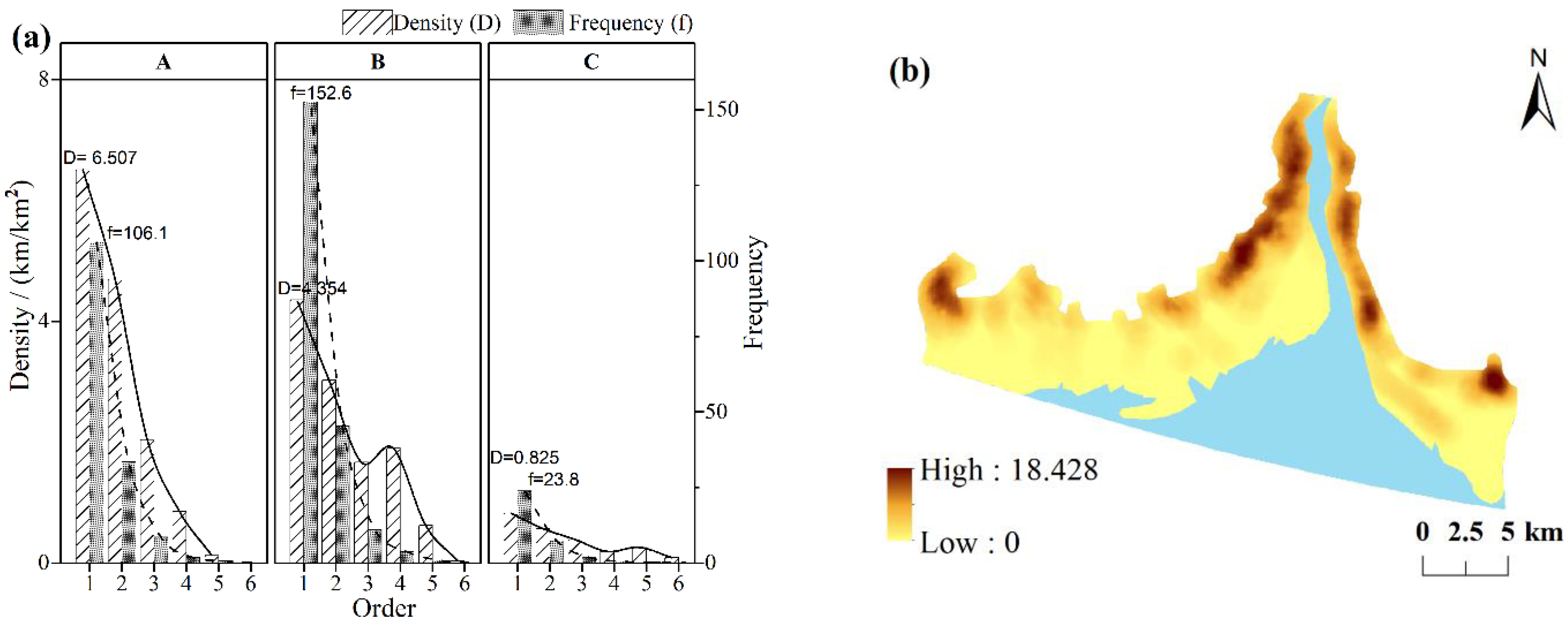
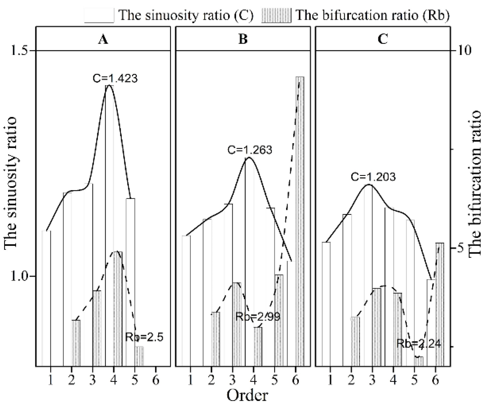
3.1. Morphological Characteristics of Tidal Creeks

In the tidal flat of estuary deltas, the morphological characteristics of tidal creeks are quite different because of the topographic elevation change. To demonstrate the differences in the morphological characteristics of the tidal flats of the LRE in detail, our study divided them into several typical areas. Figure 7 shows the order of the tidal creeks in the three regions. In the LRE, the Yuanyang island (Figure 7A), the south of the East Bank (Figure 7B), and the middle of the West Bank (Figure 7C) represent the supratidal zone (a), the upper intertidal zone (b), and the middle intertidal zone (c), respectively. In this region of the Yuanyang island, the tidal creeks are densely distributed in the tidal flat, with a high ratio of tidal creek branches for orders 1 to 3, and the main tidal creeks, for orders 4 and 5, present a short-branched type. In the south of the East Bank of the LRE, order 6 tidal creeks are also present. The main tidal creeks for orders 4 and 5 are in high ratio, and most of them are distributed on the tidal flat in an island shape. In the middle of the West Bank of the LRE, the tidal creek branches are short and sparsely distributed but the main tidal creeks are relatively long because of the influence of tidal hydrodynamics. In the study area, most of the tidal creeks have developed in the shape of a “tidal tree”, where the tidal creek branches are concentrated near the mean high-tide level in a dendritic pattern and the main tidal creeks are perpendicular to the shoreline and disappear near the average low-tide level in a pattern similar to the main trunk of a tree. According to the principles of genetic classification proposed by Shao et al. [50], the tidal creeks on a tidal flat of the LRE are scoured by the tidal currents.
The average length of tidal creeks reflects the dynamic status of the tidal flat, and the number of tidal creeks shows the density of the tidal creeks. Figure 8a shows the average length and number of tidal creeks for orders 1 to 6 in the three tidal zones. In the supratidal zone, the average lengths of tidal creek branches for orders 1 to 3 are 0.061 km, 0.14 km, and 0.239 km, respectively, the longest in the LRE. In the upper intertidal zone, the average length of tidal creeks for orders 1 to 5 gradually increases but the average length of order 6 tidal creeks (creeks of the highest order) declines significantly. In the middle intertidal zone, tidal creeks of the highest order are those of order 6, and the average lengths of tidal creeks for orders 5 and 6 are 1.21 km and 2.142 km, respectively, making them the longest in the LRE. The average length of the tidal creeks for orders 1 to 6 gradually increases in the middle intertidal zone. Our study found that tidal creeks are mainly concentrated in the upper intertidal zone (7037 in total), accounting for 50% of the total number of tidal creeks in the LRE. In the middle intertidal zone, the number of tidal creeks of orders 5 and 6 accounts for 58% of the total number of tidal creeks of the same level in this region. In the middle intertidal zone, the number of tidal creeks decreases significantly with an increase in the order of tidal creeks. In the study area, the average length and number of the main tidal creeks for orders 5 and 6 exhibit increasing trends with a declining beach surface elevation gradient. Figure 8b shows the fitting analysis between the average length, the number, and the order of tidal creeks in the coastal wetlands of the LRE. With an increase in the order of the tidal creeks, the average length of tidal creeks in the study area increases exponentially, but the number of tidal creeks decreases exponentially (R2 > 0.99). Our result is consistent with the law of river length provided by Horton, indicating that the average length and number of tidal creeks show an exponential function with increasing order [45].
The density and frequency of tidal creeks are important factors for evaluating the morphological characteristics of a tidal flat. Figure 9a shows the density and frequency of tidal creeks for orders 1 to 6 in each tidal zone. The density of tidal creeks for orders 1 to 3 in the supratidal zone is higher than that in other zones, where the highest value is 6.507 km/km2 of order 1 tidal creeks. The density of order 1 tidal creeks in the upper intertidal zone is 4.354 km/km2, and the density of tidal creeks for orders 1 to 3 in the middle intertidal zone is lower than that in other zones. The frequency of tidal creeks for orders 1 to 6 in the upper intertidal zone is higher than that in other zones, the highest value being 152.6 for order 1 tidal creeks. However, the frequency of tidal creeks for orders 1 to 6 in the middle intertidal zone is generally lower than that in other zones. In addition, the density and frequency of tidal creeks in the three tidal zones decrease with increasing order. Figure 9b shows the spatial distribution of the total density of tidal creeks in the LRE. The total density of tidal creeks ranges from 0 to 18.43 km/km2. The total densities of tidal creeks in the supratidal zone, the upper intertidal zone, and the middle intertidal zone are 14.22 km/km2, 11.61 km/km2, and 2.32 km/km2, respectively. The coastal wetlands of the LRE have a wide bell-like mouth, and the terrain is high in the north and low in the south. It is mainly composed of beaches on both banks, an island, multiple shoals, and open waters. On both banks of the study area, the total density of tidal creeks decreased dramatically from north to south, and the total density of tidal creeks inshore is higher than that offshore. Overall, the density of tidal creeks decreases significantly with a declining beach surface elevation gradient.
The sinuosity ratio of tidal creeks represents how much a tidal creek meanders, and the bifurcation ratio of tidal creeks reflects the stability of a tidal creek. Figure 10 shows the sinuosity ratio and the bifurcation ratio of tidal creeks for orders 1 to 6 in each tidal zone. In the supratidal zone, the sinuosity ratios of tidal creeks for orders 1 to 6 are higher than those in other zones, where the highest value is 1.423 for order 4 tidal creeks. In the middle intertidal zone, the sinuosity ratios of tidal creeks of orders 1 to 6 are generally the lowest, where the minimum value is approximately equal to 1 for order 6 tidal creeks. Therefore, the sinuosity ratios of the tidal creeks in the three zones can be ordered as follows: the supratidal zone > the upper intertidal zone > the middle intertidal zone. In the study area, the bifurcation ratio for order 6 tidal creeks in the upper intertidal zone is the highest (Rb = 9.33), while the bifurcation ratio for order 5 tidal creeks in the middle intertidal zone is the lowest (Rb = 2.24). According to the average bifurcation ratio for a river system obtained by arithmetically averaging the order-by-order ratios proposed by Strahler et al. [47], our study calculated the average bifurcation ratios of tidal creeks in the supratidal zone, the upper intertidal zone, and the middle intertidal zone. The values obtained were 3.42, 3.54, and 3.43, respectively, which can be ordered as follows: the upper intertidal zone > the middle intertidal zone > the supratidal zone. In the study area, the sinuosity ratios of tidal creeks for orders 1 to 3 gradually increase and reach the highest value in tidal creeks for orders 3 and 4. Then, the sinuosity ratios of tidal creeks of orders 5 and 6 decrease sharply, reaching a value close to 1.

3.2. Properties of a Tidal Creek Network

Connectivity parameters (α, β, and γ) reflect the hydrological connectivity of the tidal creek system. The value ranges of α, β, and γ are 0~1, 0~3, and 0~1, respectively. An α value of 0 means a tidal creek network without island-shaped tidal creeks, whereas an α value of 1 means a tidal creek network with the maximum number of island-shaped tidal creeks. More connections per node in a creek in the network means a β value closer to 3. When γ is equal to 0, it means that none of the nodes are connected, a γ value close to 1/3 means that the tidal creek network has a tree-like shape, whereas a γ value equal to 1 means that each node in the tidal creek network is connected to the others. Each node of a tidal creek network has better connectivity when the γ value is closer to 1 [5]. The fractal dimension (F) represents the complexity of a tidal creek system, with values ranging from 1 to 2. An F value greater than 1 indicates that the tidal creek network is self-similar. A larger F value indicates that the complexity of the tidal creek network is greater. A delta with F close to 1 has a tidal creek of a simple pattern (low density). A delta with F close to 2 would have a tidal creek network that is space filling (high density) [48].
Figure 11 gives the connectivity and fractal dimension of the tidal creek network in each tidal zone in the LRE. In the supratidal zone, the connectivity of the tidal creek network is the lowest but the fractal dimension of the tidal creek network is the highest (F = 1.56). In the upper intertidal zone, the connectivity of the tidal creek network is the highest (the values of α, β, and γ are 0.49, 1.98, and 0.66, respectively) and the fractal dimension of the tidal creek network is equal to 1.51. In the middle intertidal zone, the connectivity of the tidal creek network is higher than that in the supratidal zone but lower than that in the upper intertidal zone. The fractal dimension of the tidal creek network is the lowest (F = 1.3) in the middle intertidal zone, suggesting that the fractal dimension of the tidal creek network decreases significantly with a declining beach surface elevation gradient. Overall, in the coastal wetlands of the LRE, the tidal creek system in the upper intertidal zone has the strongest hydrological connectivity but the tidal creek system in the supratidal zone is the most complex.

4. Discussion

4.1. Analysis of the Morphological Characteristics of Tidal Creeks

Similar to the Yellow River Estuary [6], our study area was also dominated by erosion, and the degree of beach surface erosion imparted by the tidal current is controlled by the beach surface elevation gradient [51]. In the initial stage of the tidal creek development, most of the tidal creeks extended rapidly on the tidal flat through traceable erosion, resulting in a tree-like shape that eventually resulted in a stable tidal creek network. Moreover, the acceleration of sediment deposition in the runoff process improved the growth of tidal creeks [52]. In the supratidal zone and the upper intertidal zone of the LRE, the average length of tidal creeks increased with increasing order, except in the case of the highest order, which was mainly due to the instability and the width limits of the tidal flat [27,53]. Tidal creeks of the highest order in the upper and middle intertidal zones were those of order 6, while the tidal creeks in the supratidal zone were only developed up to order 5, and most of them were tidal creek branches for orders 1 to 3. This is because the terminal tidal creeks extend rapidly under the influence of traceable erosion, resulting in a high ratio of the tidal creek branches for orders 1 to 3 in the supratidal zone [26]. The average length and number of tidal creeks for orders 5 and 6 in the middle intertidal zone were the highest in the LRE, perhaps because the high-intensity tidal hydrodynamics may help in developing the main tidal creeks offshore. Overall, the order and average length of tidal creeks in coastal wetlands of the LRE demonstrated significant spatial heterogeneity. The total density of tidal creeks declined dramatically with a falling beach surface elevation gradient, consistent with the conclusions of Strahler et al. [54]. The main reason is as follows: under the action of high-intensity hydrodynamics, it was difficult for the offshore tidal creeks in the middle intertidal zone to construct a stable branching tidal creek network, resulting in the lowest density and frequency of tidal creeks for orders 1 to 3 in the LRE. The tidal hydrodynamic weakened as the beach surface elevation gradient rose, promoting the development of tidal creek branches, resulting in a significant increase in the density of tidal creek branches in the supratidal zone. Therefore, the density of tidal creeks was determined by the tidal hydrodynamic. The frequent inundation in the upper intertidal zone by tidal currents also advanced the transformation process between tidal creek branches and main tidal creeks [55]; as a result, the frequency of tidal creeks in the upper intertidal zone was higher than that in other zones. The meandering evolution of a tidal creek is regulated by the flow path during flood and ebb tides, and the sinuosity ratio of tidal creeks of different orders in the LRE can be ordered as follows: orders 3 and 4 > orders 1 and 2 > orders 5 and 6. The main reasons are as follows: With the influence of seawater erosion and sediment siltation and the instability and low curvature of tidal creeks for orders 1 and 2, they were easily transformed into tidal creeks for orders 3 and 4, with relative stability. With increasing two-direction flow velocity, the sinuosity ratios of tidal creeks for orders 3 and 4 increased significantly, transforming them into main tidal creeks for orders 5 and 6. The tidal creeks for orders 5 and 6 display the phenomenon of “curving cut-off”, probably because the tidal currents in the tidal creek increased dramatically during storm surges and rainstorms. This higher flow results in tidal creek cutting, bending, and straightening, which ultimately reduces its sinuosity ratio to a value close to 1 [6,56]. In addition, the sinuosity ratios of tidal creek zones decreased dramatically from the supratidal zone to the upper intertidal zone, to the middle intertidal zone, consistent with the conclusion proposed by Marani et al. [57] that the sinuosity ratio of offshore tidal creeks is lower than that of inshore ones. The lower sinuosity ratio of tidal creeks in the middle intertidal zone was caused by the increase in the number of tidal creeks for orders 5 and 6 and the high-intensity offshore tidal currents. With the frequent conversions of tidal creeks between low-order ones and high-order ones, the average bifurcation ratio of the tidal creeks in the upper intertidal zone was higher than that in other zones, indicating that the tidal creeks in the upper intertidal zone are quite erratic. As a result, the sinuosity ratio and the bifurcation ratio of tidal creeks were mainly regulated by the hydrodynamic intensity.

4.2. Evaluation of the Complexity and Hydrological Connectivity of the Tidal Creek Network

Similar to the average bifurcation ratio of tidal creeks, the hydrological connectivity of tidal creek networks in the three tidal zones can be ordered as follows: the supratidal zone < the middle intertidal zone < the upper intertidal zone. This is mainly because the upper intertidal zone is frequently inundated by tidal currents, promoting the development of the island-shaped tidal creeks and resulting in the strongest hydrological connectivity of the tidal creek network in this zone. Similar to the findings of Yu et al. [20], the connectivity indices in the Yellow River Estuary were determined by the number of island-shaped tidal creeks and the ratios of the nodes connected in a tidal creek network. Therefore, the hydrological connectivity of the tidal creek network in LRE was positively correlated with both the average bifurcation ratio of the tidal creeks and the number of island-shaped tidal creeks. The fractal dimension of the tidal creek network in three tidal zones can be ordered as follows: the supratidal zone > the upper intertidal zone > the middle intertidal zone. This suggests that the complexity of the offshore tidal creek system was inferior to that of the inshore one. However, the F value of the tidal creek network in the middle intertidal zone was only 1.3, which does not conform to the standard proposed by LaBarbera et al., that the typical fractal dimension of the hydrographic net should be between 1.5 and 2.0 [58]. This is because the tidal creeks in the middle intertidal zone were seriously scoured by the seawater, making it impossible for the creeks to develop a complex tidal channel network. Similar to the fractal dimension of the tidal creek network, the sinuosity ratio of tidal creeks and the total density of tidal creeks in the three tidal zones can be ordered as follows: the supratidal zone > the upper intertidal zone > the middle intertidal zone. Our study can conclude that the fractal dimension of the tidal creek network in the LRE was regulated by the sinuosity ratio and total density of tidal creeks, which is consistent with Eom’s supposition [22,59]. Overall, the hydrological connectivity of the tidal creek network was gradually enhanced with an increasing average bifurcation ratio of tidal creeks and the number of island-shaped tidal creeks. The complexity of the tidal creek system steadily grew with an increasing sinuosity ratio and total density of tidal creeks.

5. Conclusions

Our study proposed an integral framework for tidal flat zonation, tidal creek extraction, and morphological characteristic evaluation in the coastal wetlands using high-resolution RS data. Using the automatic framework algorithm, our study quantitatively analyzed the variation in tidal creek morphology and qualitatively evaluated the hydrological connectivity and complexity of the tidal creek system in three tidal zones of the coastal wetlands in LRE.
(1)
The tidal creeks on the tidal flat of the LRE were scoured by tidal currents. The main tidal creeks and tributaries of the tidal flat were linked together in the shape of a “tidal tree.” The tidal creek branches were concentrated near the mean high-tide level in a dendritic pattern, and the main tidal creeks were perpendicular to the shoreline and disappeared near the average low-tide level in a pattern similar to the main trunk of a tree.
(2)
In the study area, there was obvious spatial heterogeneity in the order and average length of the tidal creeks. The level of tidal creeks in the upper and middle intertidal zones was higher than in the supratidal zone. In the study area, with an increase in the order of tidal creeks, the average length of tidal creeks increased exponentially but the number of tidal creeks decreased exponentially (R2 > 0.99). The total density of tidal creeks declined dramatically with a decreasing beach surface elevation gradient. In addition, as the hydrodynamic intensities on the tidal flat differed, the sinuosity ratio of offshore tidal creeks was lower than that of inshore ones and the average bifurcation ratio of the tidal creeks in the upper intertidal zone (Rb = 3.54) was the highest in the LRE.
(3)
In the coastal wetlands of the LRE, the properties of the tidal creek network and the morphological characteristics of tidal creeks were interconnected. The connectivity of the tidal creek network was positively correlated with the average bifurcation ratio of tidal creeks and the number of island-shaped tidal creeks. The fractal dimension of the tidal creek network was regulated by the sinuosity ratio and total density of tidal creeks. In the study area, the tidal creek network in the upper intertidal zone had the strongest hydrological connectivity and the tidal creek system in the supratidal zone was the most complex, with an F value of 1.56.
We believe that the framework approach taken in this study could help in the improvement and semi-automatic interpretation of morphological characteristics and hydrological connectivity of tidal creek networks. Although the results pertain to a specific geographical area, the extraction method and analytical procedures are potentially applicable to other tidal wetlands and could help to understand the relationship between the tidal creek system and tidal hydrodynamics. In the future, we will explore the interaction between tidal creeks, vegetation, and hydrodynamics.

Author Contributions

Conceptualization, M.Z. and X.C.; methodology, M.Z. and X.C.; software, X.C.; validation, H.J. and X.C.; formal analysis, H.J. and X.C.; investigation, H.J. and X.C.; resources, H.J. and X.C.; data curation, H.J. and X.C.; writing—original draft preparation, M.Z.; writing—review and editing, M.Z.; supervision, M.Z. All authors have read and agreed to the published version of the manuscript.

Funding

This research was funded by the National Nature Science Foundation of China, grant numbers 51879028 and U21A20155; Guidance Program of Liaoning Province Natural Fund, grant numbers 2019-ZD-0729.

Institutional Review Board Statement

Not applicable.

Informed Consent Statement

Not applicable.

Data Availability Statement

The data presented in this study are available on request from the corresponding author.

Conflicts of Interest

The authors declare no conflict of interest.

References

  1. Kirwan, M.L.; Megonigal, J.P. Tidal wetland stability in the face of human impacts and sea-level rise. Nature 2013, 504, 53–60. [Google Scholar] [CrossRef] [PubMed]
  2. Guan, B.; Gao, N.; Chen, M.; Cagle, G.A.; Hou, A.; Han, G.; Tian, X. Seedling adaptive characteristics of Phragmites australis to nutrient heterogeneity under salt stress using a split-root approach. Aquat. Sci. 2021, 83, 1–11. [Google Scholar] [CrossRef]
  3. Rogers, K.; Saintilan, N.; Copeland, C. Managed retreat of saline coastal wetlands: Challenges and opportunities identified from the Hunter River Estuary, Australia. Estuaries Coasts 2014, 37, 67–78. [Google Scholar] [CrossRef] [Green Version]
  4. Pestrong, R. The Development of Drainage Patterns on Tidal Marshes; Stanford University: Stanford, CA, USA, 1965. [Google Scholar]
  5. Yu, X.; Zhang, Z.; Xue, Z.; Wu, H.; Zhang, H. Effects of tidal channels and roads on landscape dynamic distribution in the Yellow River Delta, China. Chin. Geograp. Sci. 2020, 30, 170–179. [Google Scholar] [CrossRef] [Green Version]
  6. Gong, Z.; Mou, K.; Wang, Q.; Qiu, H.; Zhang, C.; Zhou, D. Parameterizing the Yellow River Delta tidal creek morphology using automated extraction from remote sensing images. Sci. Total Environ. 2021, 769, 144572. [Google Scholar] [CrossRef]
  7. Agudo, P.; Sámano, M.L.; Rodríguez, A.; Crespo, J.; Masías, M.; Dzul, L.; Gracia, S. Validation of a methodology to analyze the morphological parameters in newly created tidal channels through a video monitoring system. Appl. Sci. 2019, 9, 796. [Google Scholar] [CrossRef] [Green Version]
  8. Vijay, R.; Dey, J.; Sakhre, S.; Kumar, R. Impact of urbanization on creeks of Mumbai, India: A geospatial assessment approach. J. Coast. Conserv. 2020, 24, 1–16. [Google Scholar] [CrossRef]
  9. Park, C.; Yu, J.; Kim, J.; Yang, D.Y. Monitoring variation of tidal channels associated with Shihwa reclamation project using remote sensing approaches. Econ. Environ. Geol. 2019, 52, 299–312. [Google Scholar]
  10. Shi, Z.; Lamb, H.F.; Collin, R.L. Geomorphic change of saltmarsh tidal creek networks in the Dyfi Estuary, Wales. Mar. Geol. 1995, 128, 73–83. [Google Scholar] [CrossRef]
  11. Temmerman, S.; Meire, P.; Bouma, T.J.; Herman, P.M.J.; Ysebaert, T.; De Vriend, H.J. Ecosystem-based coastal defence in the face of global change. Nature 2013, 504, 79–83. [Google Scholar] [CrossRef]
  12. Xie, C.; Cui, B.; Xie, T.; Yu, S.; Liu, Z.; Chen, C.; Ning, Z.; Wang, Q.; Zou, Y.; Shao, X. Hydrological connectivity dynamics of tidal flat systems impacted by severe reclamation in the Yellow River Delta. Sci. Total Environ. 2020, 739, 139860. [Google Scholar] [CrossRef] [PubMed]
  13. Goudie, A. Characterising the distribution and morphology of creeks and pans on salt marshes in England and Wales using Google Earth. Estuar. Coast. Shelf Sci. 2013, 129, 112–123. [Google Scholar] [CrossRef]
  14. Hood, W.G. Tidal channel meander formation by depositional rather than erosional processes: Examples from the prograding Skagit River Delta (Washington, USA). Earth Surf. Process. Landf. J. Br. Geomorphol. Res. Group 2010, 35, 319–330. [Google Scholar] [CrossRef]
  15. Passalacqua, P.; Trung, T.D.; Foufoula-Georgiou, E.; Sapiro, G.; Dietrich, W.E. A geometric framework for channel network extraction from lidar: Nonlinear diffusion and geodesic paths. J. Geophys. Res. Earth Surf. 2010, 115, F01002. [Google Scholar] [CrossRef] [Green Version]
  16. Chirol, C.; Haigh, I.; Pontee, N.; Thompson, C.; Gallop, S. Parametrizing tidal creek morphology in mature saltmarshes using semi-automated extraction from lidar. Remote Sens. Environ. 2018, 209, 291–311. [Google Scholar] [CrossRef]
  17. Limaye, A.B. Extraction of multithread channel networks with a reduced-complexity flow model. J. Geophys. Res. Earth Surf. 2017, 122, 1972–1990. [Google Scholar] [CrossRef]
  18. Mason, D.C.; Scott, T.R.; Wang, H.J. Extraction of tidal channel networks from airborne scanning laser altimetry. ISPRS J. Photogramm. Remote Sens. 2006, 61, 67–83. [Google Scholar] [CrossRef]
  19. Hiatt, M.; Sonke, W.; Addink, E.A.; van Dijk, W.M.; van Kreveld, M.; Ophelders, T.; Verbeek, K.; Vlaming, J.; Speckmann, B.; Kleinhans, M.G. Geometry and topology of estuary and braided river channel networks automatically extracted from topographic data. J. Geophys. Res. Earth Surf. 2020, 125, e2019JF005206. [Google Scholar] [CrossRef] [Green Version]
  20. Yu, X.; Zhang, Z.; Xue, Z.; Song, X.; Zhang, H.; Wu, H. Morphological characteristics and connectivity of tidal channels in the Yellow River Delta for 7 periods since 1989. Wetl. Sci. 2018, 16, 517–523. [Google Scholar]
  21. Passalacqua, P.; Lanzoni, S.; Paola, C.; Rinaldo, A. Geomorphic signatures of deltaic processes and vegetation: The Ganges-Brahmaputra-Jamuna case study. J. Geophys. Res. Earth Surf. 2013, 118, 1838–1849. [Google Scholar] [CrossRef]
  22. Eom, J.; Choi, J.K.; Ryu, J.H.; Woo, H.J.; Won, J.S.; Jang, S. Tidal channel distribution in relation to surface sedimentary facies based on remotely sensed data. Geosci. J. 2012, 16, 127–137. [Google Scholar] [CrossRef]
  23. Fagherazzi, S.; Kirwan, M.L.; Mudd, S.M.; Guntenspergen, G.R.; Temmerman, S.; D’Alpaos, A.; Van De Koppel, J.; Rybczyk, J.M.; Reyes, E.; Craft, C.; et al. Numerical models of salt marsh evolution: Ecological, geomorphic, and climatic factors. Rev. Geophys. 2012, 50, RG1002. [Google Scholar] [CrossRef]
  24. Kim, D.; Cairns, D.M.; Bartholdy, J. Tidal creek morphology and sediment type influence spatial trends in salt marsh vegetation. Prof. Geogr. 2013, 65, 544–560. [Google Scholar] [CrossRef]
  25. Tambroni, N.; Bolla Pittaluga, M.; Seminara, G. Laboratory observations of the morphodynamic evolution of tidal channels and tidal inlets. J. Geophys. Res. Earth Surf. 2005, 110, F04009. [Google Scholar] [CrossRef] [Green Version]
  26. Stefanon, L.; Carniello, L.; D’Alpaos, A.; Lanzoni, S. Experimental analysis of tidal network growth and development. Cont. Shelf Res. 2010, 30, 950–962. [Google Scholar] [CrossRef] [Green Version]
  27. Zhao, B.; Liu, Y.; Xu, W.; Liu, Y.; Sun, J.; Wang, L. Morphological characteristics of tidal creeks in the central coastal region of Jiangsu, China, using LiDAR. Remote Sens. 2019, 11, 2426. [Google Scholar] [CrossRef] [Green Version]
  28. Vlaswinkel, B.M.; Cantelli, A. Geometric characteristics and evolution of a tidal channel network in experimental setting. Earth Surf. Process. Landf. 2011, 36, 739–752. [Google Scholar] [CrossRef]
  29. Seminara, G.; Lanzoni, S.; Tambroni, N.; Toffolon, M. How long are tidal channels? J. Fluid Mech. 2010, 643, 479–494. [Google Scholar] [CrossRef] [Green Version]
  30. Vandenbruwaene, W.; Bouma, T.J.; Meire, P.; Temmerman, S. Bio-geomorphic effects on tidal channel evolution: Impact of vegetation establishment and tidal prism change. Earth Surf. Process. Landf. 2013, 38, 122–132. [Google Scholar] [CrossRef]
  31. Davies, G.; Woodroffe, C.D. Tidal estuary width convergence: Theory and form in North Australian estuaries. Earth Surf. Process. Landf. J. Br. Geomorphol. Res. Group 2010, 35, 737–749. [Google Scholar] [CrossRef]
  32. Florinsky, I.V. Quantitative topographic method of fault morphology recognition. Geomorphology 1996, 16, 103–119. [Google Scholar] [CrossRef]
  33. Qu, Z.; Li, Y.; Yu, J.; Yang, J.; Yu, M.; Zhou, D.; Wang, X.; Wang, Z.; Yu, Y.; Ma, Y.; et al. Influence of gate dams on Yellow River Delta Wetlands. Land 2022, 11, 706. [Google Scholar] [CrossRef]
  34. Bracken, L.J.; Croke, J. The concept of hydrological connectivity and its contribution to understanding runoff-dominated geomorphic system. Hydrol. Process. Int. J. 2007, 21, 1749–1763. [Google Scholar] [CrossRef]
  35. Deng, X.; Xu, Y.; Han, L. Impacts of human activities on the structural and functional connectivity of a river network in the Taihu Plain. Land Degrad. Dev. 2018, 29, 2575–2588. [Google Scholar] [CrossRef]
  36. Feng, J.; Liang, J.; Li, Q.; Zhang, X.; Yue, Y.; Gao, J. Effect of hydrological connectivity on soil carbon storage in the Yellow River delta wetlands of China. Chin. Geogr. Sci. 2021, 31, 197–208. [Google Scholar] [CrossRef]
  37. Zhang, M.; Xu, T.; Jiang, H. The impacts of runoff decrease and shoreline change on the salinity distribution in the wetlands of Liao River estuary, China. Ocean Sci. 2021, 17, 187–201. [Google Scholar] [CrossRef]
  38. Zhang, J.; Zhang, Y.; Lloyd, H.; Zhang, Z.; Li, D. Rapid reclamation and degradation of suaeda salsa saltmarsh along coastal China’s Northern Yellow Sea. Land 2021, 10, 835. [Google Scholar] [CrossRef]
  39. Fu, B.; Zuo, P.; Liu, M.; Lan, G.; He, H.; Lao, Z.; Zhang, Y.; Fan, D.; Gao, E. Classifying vegetation communities karst wetland synergistic use of image fusion and object-based machine learning algorithm with Jilin-1 and UAV multispectral images. Ecol. Indic. 2022, 140, 108989. [Google Scholar] [CrossRef]
  40. Xukai, Z.; Xia, Z.; Banghui, Y.; Zhi, Z.H.; Kun, S.H. Coastline extraction using remote sensing based on coastal type and tidal correction. Remote Sens. Land Resour. 2013, 25, 91–97. [Google Scholar]
  41. Boak, E.H.; Turner, I.L. Shoreline definition and detection: A review. J. Coast. Res. 2005, 21, 688–703. [Google Scholar] [CrossRef] [Green Version]
  42. Wu, D.L.; Shen, Y.M.; Fang, R.J. A morphological analysis of tidal creek network patterns on the central Jiangsu coast. Acta Geogr. Sinica 2013, 68, 955–965. [Google Scholar]
  43. Lv, X.; Ma, B.; Yu, J.; Chang, S.X.; Xu, J.; Li, Y.; Wang, G.; Han, G.; Bo, G.; Chu, X. Bacterial community structure and function shift along a successional series of tidal flats in the Yellow River Delta. Sci. Rep. 2016, 6, 36550. [Google Scholar] [CrossRef] [PubMed]
  44. Han, Q.Q.; Niu, Z.G. China intertidal zone dataset based on tidal correction. J. Glob. Change Data Discov. 2019, 3, 42–47. [Google Scholar]
  45. Horton, R.E. Erosional development of streams and their drainage basins; hydrophysical approach to quantitative morphology. Geol. Soc. Am. Bull. 1945, 56, 275–370. [Google Scholar] [CrossRef] [Green Version]
  46. Novakowski, K.I.; Torres, R.; Gardner, L.R.; Voulgaris, G. Geomorphic analysis of tidal creek networks. Water Resour. Res. 2004, 40, W05401. [Google Scholar] [CrossRef]
  47. Strahler, A.N. Revisions of Horton’s quantitative factors in erosional terrain. Trans. Am. Geophys. Union 1953, 34, 345. [Google Scholar]
  48. Edmonds, D.A.; Paola, C.; Hoyal, D.C.J.D.; Sheets, B.A. Quantitative metrics that describe river deltas and their channel networks. J. Geophys. Res. Earth Surf. 2011, 116, F04022. [Google Scholar] [CrossRef]
  49. Cui, B.; Wang, C.; Tao, W.; You, Z. River channel network design for drought and flood control: A case study of Xiaoqinghe River basin, Jinan City, China. J. Environ. Manag. 2009, 90, 3675–3686. [Google Scholar] [CrossRef]
  50. Shao, X.S. Genetic classification of tidal creek and factors affecting its development. Acta Geogr. Sinica 1988, 43, 35–43. [Google Scholar]
  51. Xie, D.F.; Gao, S.; Pan, C.H. Numerical simulation study on geomorphological evolution of tidal channel system. Acta Oceanol. Sin-Chinese Edit. 2010, 5, 154–161. [Google Scholar]
  52. Qiu, Z.; Xiao, C.; Perrie, W.; Sun, D.Y.; Wang, S.Q.; Shen, H.; Yang, D.Z.; He, Y.J. Using Landsat 8 data to estimate suspended particulate matter in the Yellow River estuary. J. Geophys. Res. Oceans 2017, 122, 276–290. [Google Scholar] [CrossRef]
  53. Schumm, S.A. Evolution of drainage systems and slopes in badlands at Perth Amboy, New Jersey. Geol. Soc. Am. Bull. 1956, 67, 597–646. [Google Scholar] [CrossRef]
  54. Strahler, A.N. Quantitative analysis of watershed geomorphology. Eos Transact. Am. Geophys. Union 1957, 38, 913–920. [Google Scholar] [CrossRef] [Green Version]
  55. Yan, S. The Growth and Evolution of Tidal Creeks on the Prograding Mud Flat in Jiangsu Province; Nanjing Normal University: Nanjing, China, 2002. [Google Scholar]
  56. Hibma, A.; Stive MJ, F.; Wang, Z.B. Estuarine morphodynamics. Coast. Eng. 2004, 51, 765–778. [Google Scholar] [CrossRef]
  57. Marani, M.; Lanzoni, S.; Zandolin, D.; Seminara, G.; Rinaldo, A. Tidal meanders. Water Resour. Res. 2002, 38, 7-1. [Google Scholar] [CrossRef]
  58. LaBarbera, P.R.R. On the fractal dimensions of stream network. Water Resour. Res. 1989, 25, 735–741. [Google Scholar] [CrossRef]
  59. Eom, J.A.; Choi, J.K.; Ryu, J.H.; Won, J.S. A study of tidal channel influence upon surficial sediment distribution in the Ganghwa-Do southern tidal flat. In Proceedings of the 2010 IEEE International Geoscience and Remote Sensing Symposium, Honolulu, HI, USA, 25–30 July 2010; pp. 934–937. [Google Scholar]
Figure 1. (a) The location and (b) the study area in the coastal wetlands of the Liao River Estuary.
Land 11 01707 g001
Figure 2. Sketch of the instantaneous waterline inverted by remote sensing images. ((a): The false color image, (b): Classification map, and (c): Waterline overlay image).
Land 11 01707 g002
Figure 3. Principle of tidal correction.
Land 11 01707 g003
Figure 4. Tidal correction schematic diagram using instantaneous water edges.
Land 11 01707 g004
Figure 5. The overlay map of tidal creek extraction and tidal zone division.
Land 11 01707 g005
Figure 6. Flow chart of tidal creek ordering. ((a): The tree-shaped tidal creek and (b,c): The island-shaped tidal creek).
Land 11 01707 g006
Figure 7. Distribution of tidal creeks in the coastal wetlands of the Liao River Estuary. ((a): the supratidal zone; (b): the upper intertidal zone; (c): the middle intertidal zone).
Land 11 01707 g007
Figure 8. (a) Average length-number boxplot and (b) fitting analysis of tidal creeks of different orders in the coastal wetlands of the Liao River Estuary (La: average length of tidal creeks; n: number of tidal creeks; A: the supratidal zone; B: the upper intertidal zone; C: the middle intertidal zone).
Land 11 01707 g008
Figure 9. Statistics of (a) density and frequency of tidal creeks of different orders and (b) total density of tidal creeks in the coastal wetlands of the Liao River Estuary. (A: the supratidal zone; B: the upper intertidal zone; C: the middle intertidal zone).
Land 11 01707 g009
Figure 10. Statistics of sinuosity ratios and bifurcation ratios of tidal creeks of different orders in the coastal wetlands of the Liao River Estuary. (A: the supratidal zone; B: the upper intertidal zone; C: the middle intertidal zone).
Land 11 01707 g010
Figure 11. Statistics of connectivity and fractal dimension of tidal creek networks in the coastal wetlands of the Liao River Estuary. (A: the supratidal zone; B: the upper intertidal zone; C: the middle intertidal zone).
Land 11 01707 g011
Table 1. Tidal information calculated by the remote sensing images at the scene center time.
Image DataData SourceHigh TideLow TideTidal Information
TimeTidal Level/mTimeTidal Level/mImage TimeTidal Level/mTidal Condition
29 May 2021Landsat8 OLI08:083.3014:110.4410:351.449Ebb tide
20 October 2021Landsat8 OLI06:013.6012:250.7210:351.265Ebb tide
Note: The vertical datum at the Laobeihe tide gauge station is 209 m below the local mean sea level.
Table 2. Morphological parameters of tidal creeks in the LRE and the formulas for calculating the parameters.
ParameterAbbreviationFormulaDescription
Length [6]L
Number [45]n
Density [46]D D = L A The total length of tidal creeks per unit area on the tidal flat
Frequency [45]f f = n A The total number of tidal creeks per unit area on the tidal flat
Sinuosity ratio [4]C C = L L The ratio of the length of the tidal creeks to the straight length of the tidal creeks
Bifurcation ratio [47]Rb R b = n w n w + 1 The ratio of the number of order w tidal creeks to the number of order w + 1 tidal creeks
Fractal dimension [48]F F = l i m a 0 l n N ( a ) l n a The slope of lnN(a) and ln 1/a
Network connectivity [49]α α = n v + 1 2 v 5 The ratio of the actual number of loops to the maximum number of possible loops
β β = n v The average creek number of connections per node in the network
γ γ = n n max = n 3 ( v 2 ) The ratio of the actual number of tidal creeks to the maximum number of possible tidal creeks
Note: L is the centerline length of the tidal creeks (km), ΣL is the total length of the tidal creeks (km), A is the area of the tidal flat (km2), n is the number of tidal creeks, Σn is the total number of tidal creeks, L′ is the straight length of the tidal creeks (km), nw is the number of order w tidal creeks, nw+1 is the number of order w + 1 tidal creeks, N(a) is the number of non-empty boxes that completely cover the entire figure using the square box, a is the length of the square box, and v is the number of nodes and v ≥ 3.
Publisher’s Note: MDPI stays neutral with regard to jurisdictional claims in published maps and institutional affiliations.

