


A Multi-Scenario Land Expansion Simulation Method from Ecosystem Services Perspective of Coastal Urban Agglomeration: A Case Study of GHM-GBA, China

Abstract
:1. Introduction
2. Materials and Methods
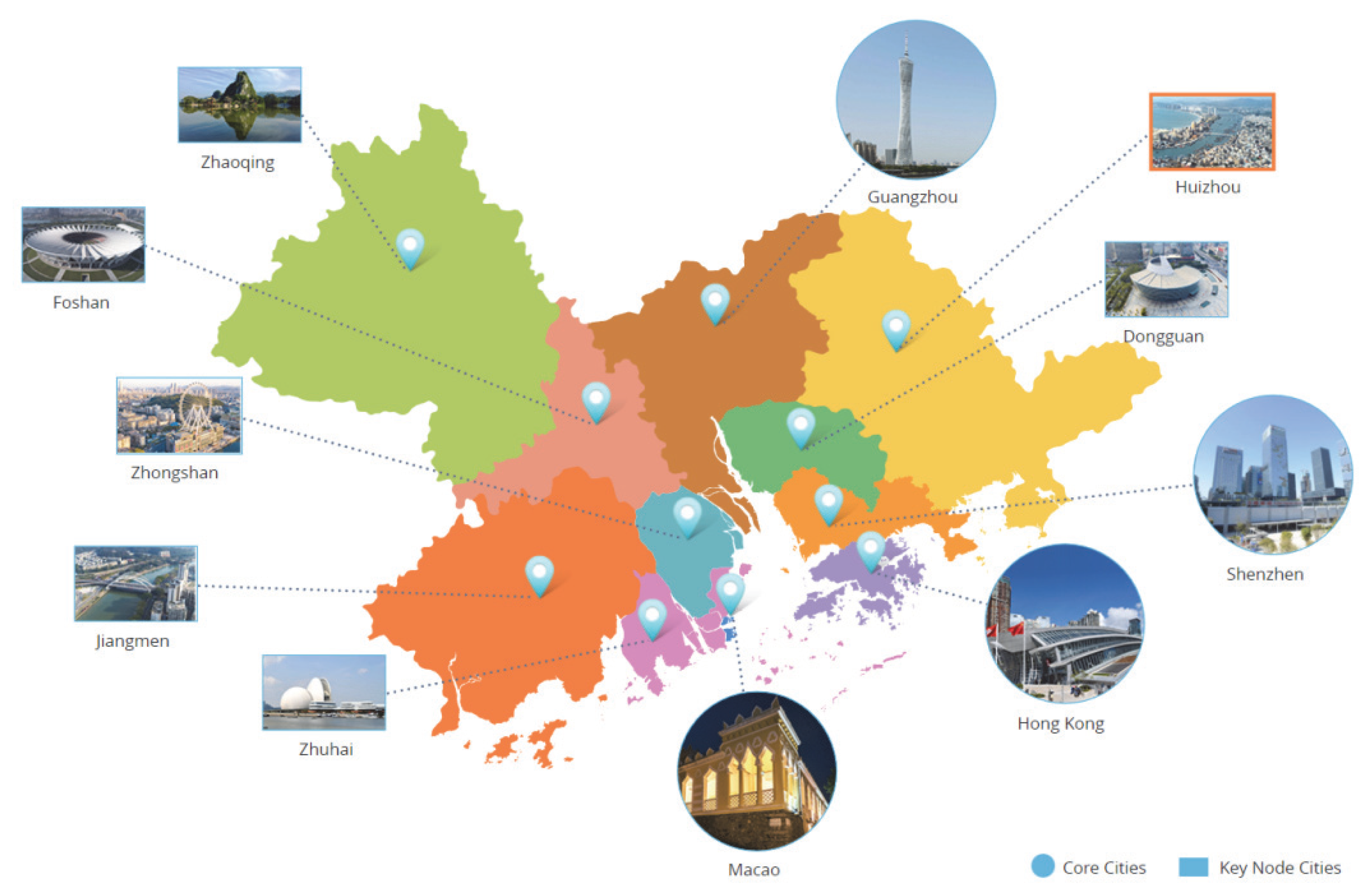
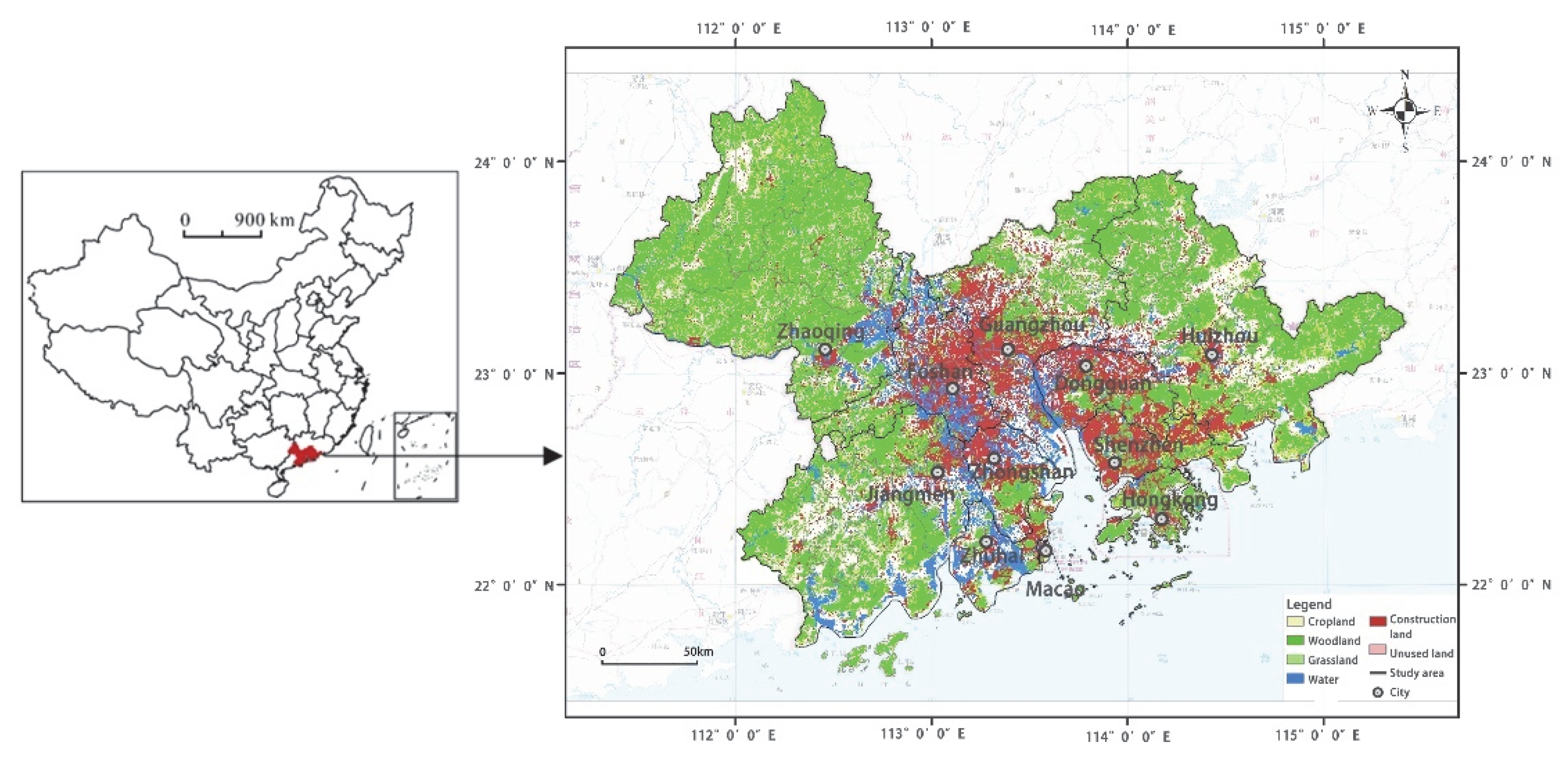
2.1. Study Area
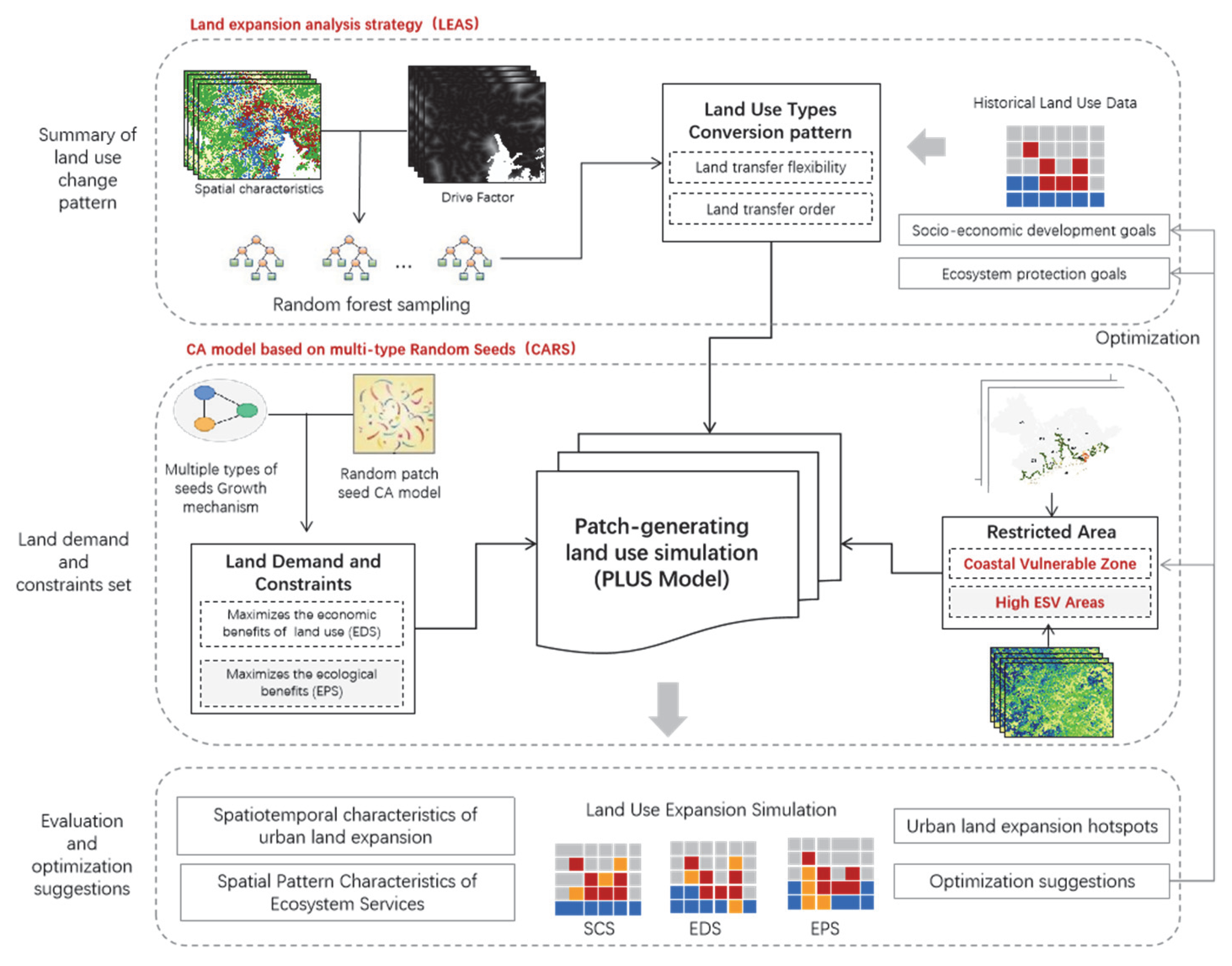
2.2. Theoretical Framework
2.3. Data Source and Processing
3. Methodology
3.1. Scenario Setting
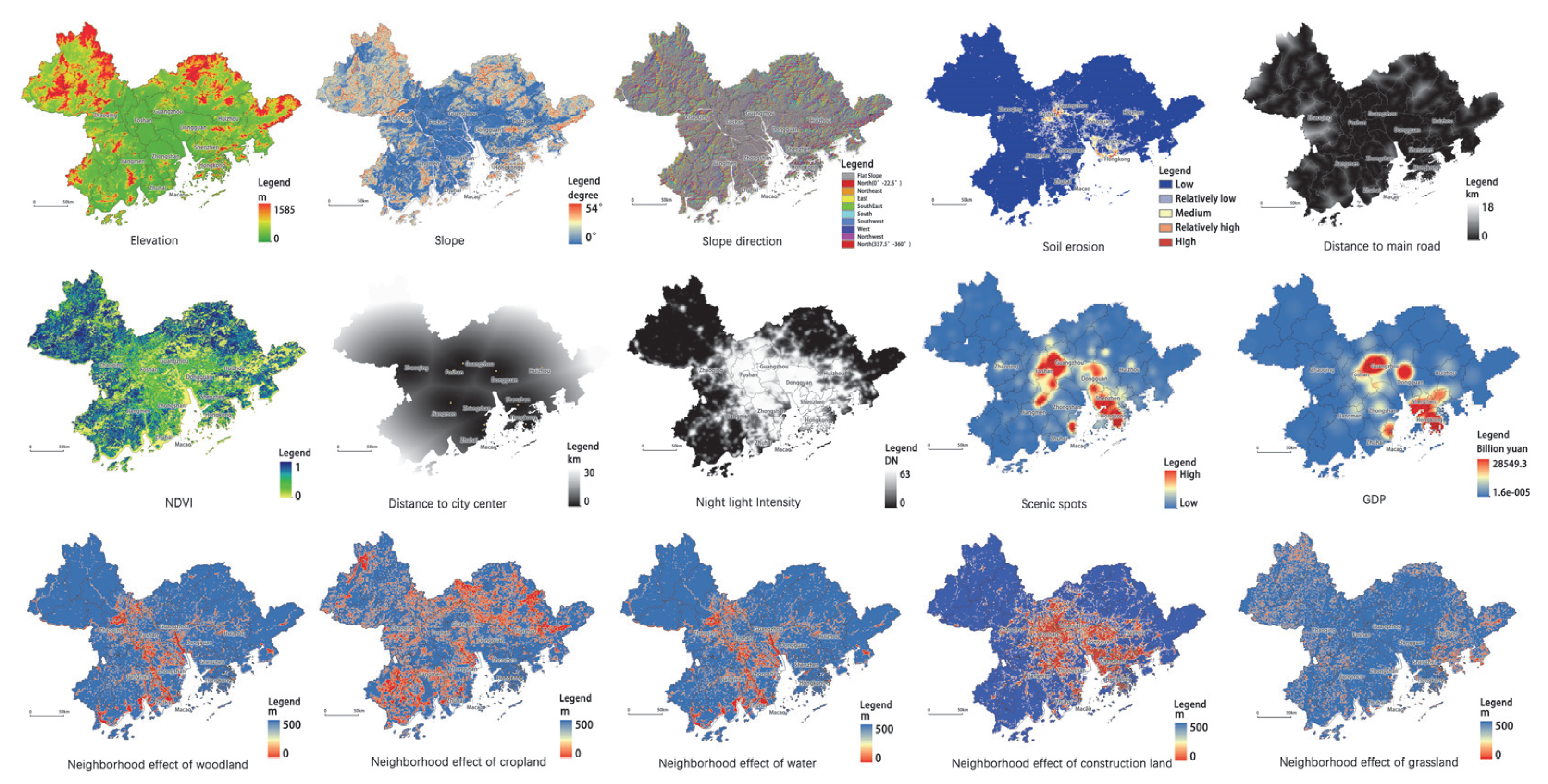
3.2. Parameter Setting for PLUS Model
3.3. Methods for Quantifying Land Use Change Patterns
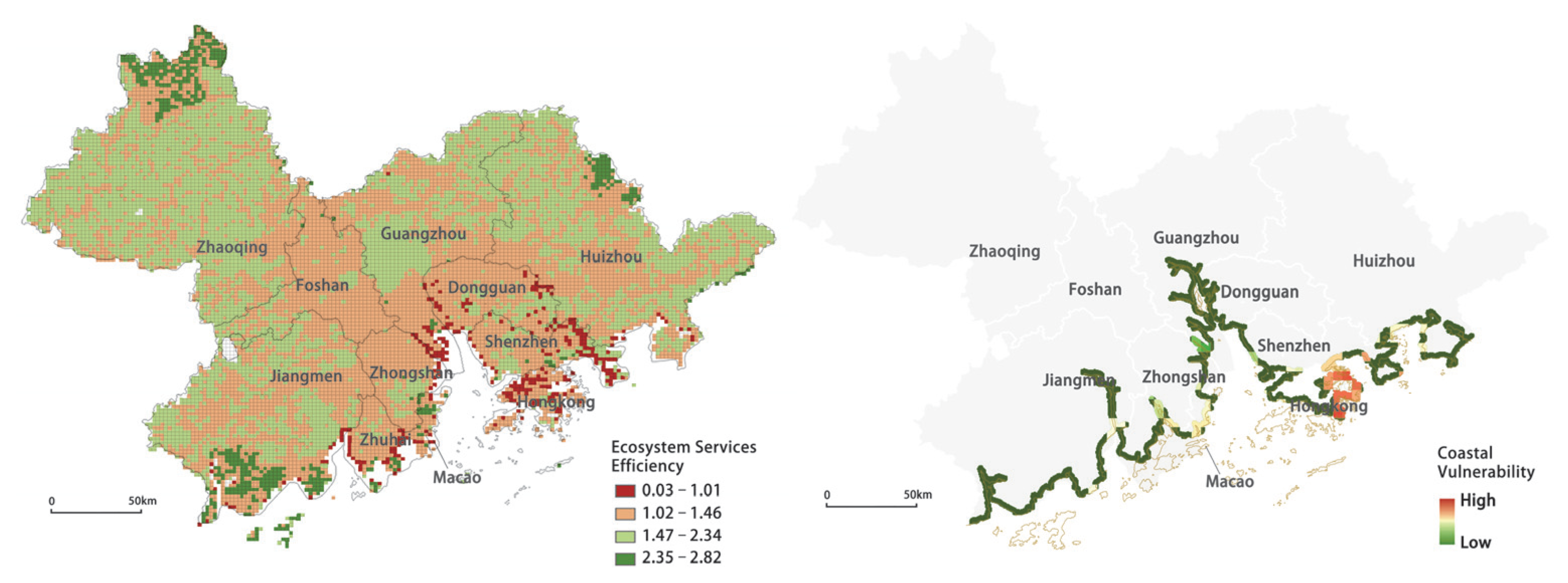
3.4. Methods for Analyzing Spatial Patterns of ES and ESV
4. Results
4.1. Step 1: Summary of Land Use Change Pattern
4.2. Step 2: Land Demand and Constraints Set for EDS and EPS
4.2.1. Land Demand, Demand Analysis, and Formula
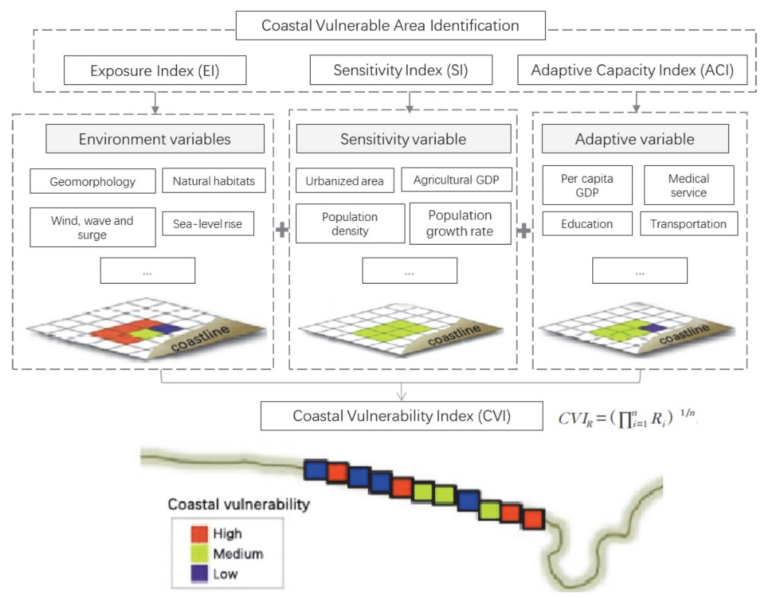
4.2.2. Restricted Area
4.3. Step 3: Land Expansion Simulation
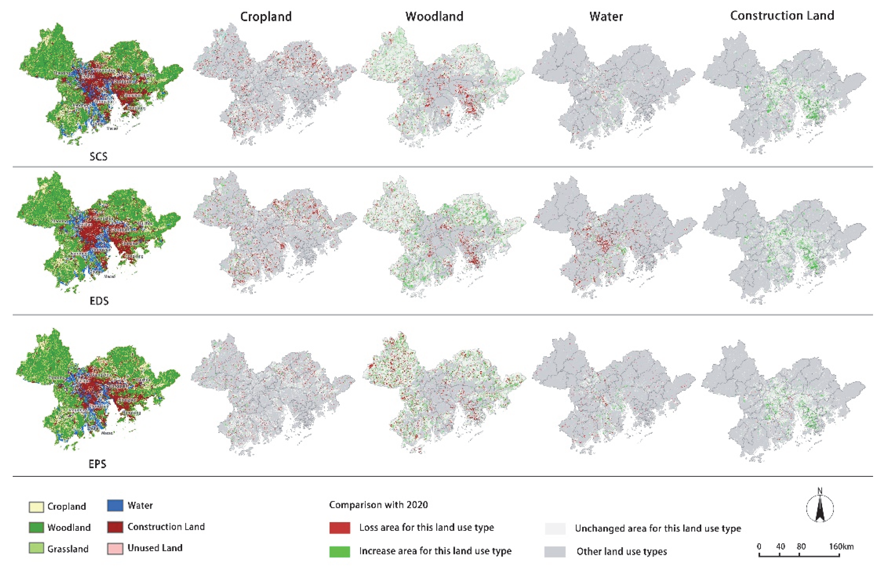
4.3.1. The Pattern of Land Expansion of Predicted Scenarios
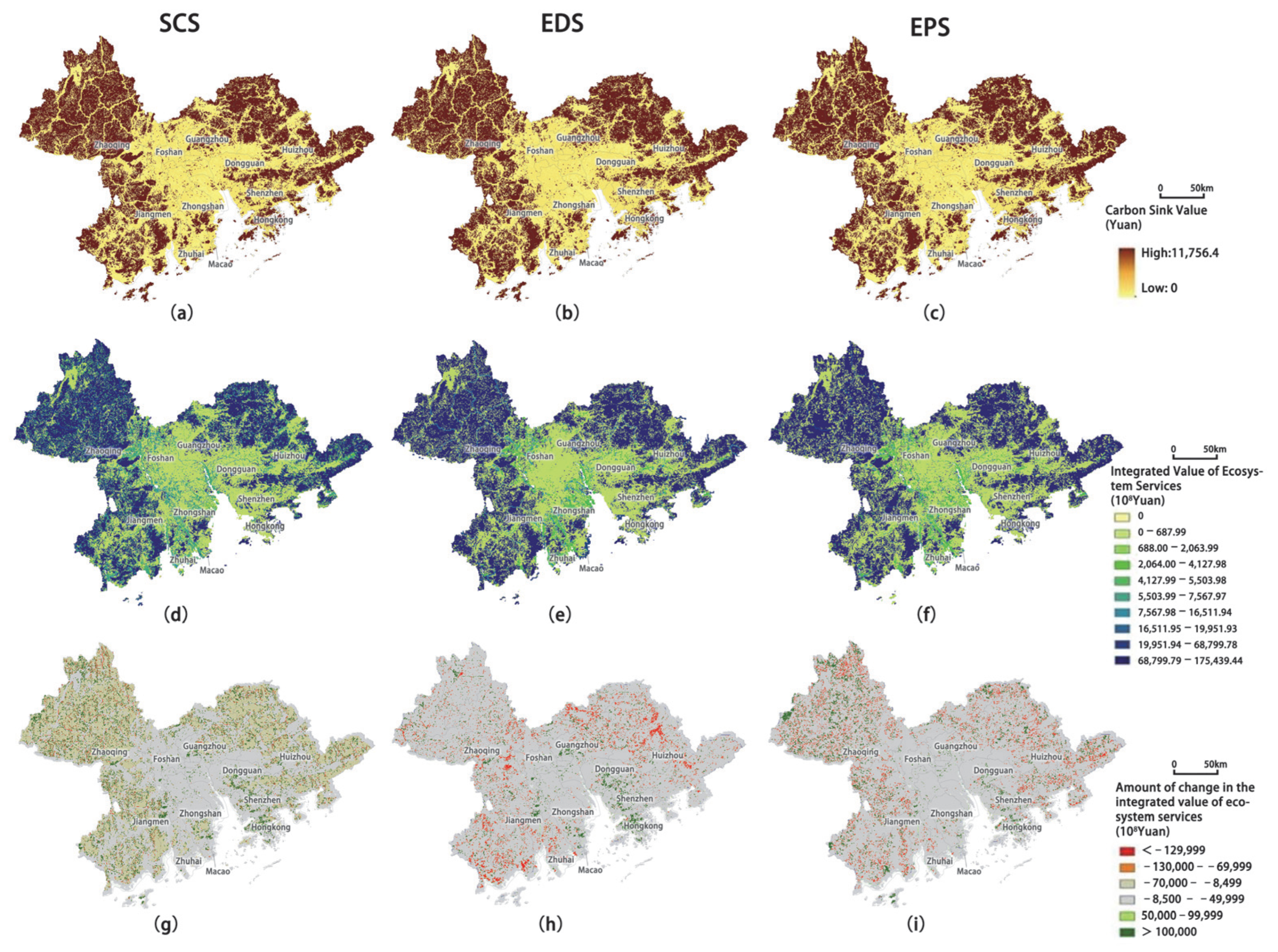
4.3.2. Ecosystem Services Characteristics of Predicted Scenarios
4.4. Analysis of the Interaction between Urban Land Expansion and Ecosystem Services
4.4.1. Correlation of Urban Land Expansion Drivers with ESVs
4.4.2. Analysis of Urban Land Expansion Hotspots and ESV Correlation
5. Discussion and Conclusions
5.1. Discussion
5.1.1. Simulation of Land Expansion from the Ecosystem Services Perspective Provides a Unified Perspective
5.1.2. Multiple Scenario Simulation Results: A possible Optimal Path to Realizing Ecological Civilization
5.1.3. Land Use Optimization Strategies for Urban Agglomeration in the GHM-GBA Based on Simulation Results
5.1.4. Study Limitations
5.2. Conclusions
Author Contributions
Funding
Data Availability Statement
Conflicts of Interest
References
- Mooney, H.; Larigauderie, A.; Cesario, M.; Elmquist, T.; Hoegh-Guldberg, O.; Lavorel, S.; Mace, G.; Palmer, M.; Scholes, R.; Yahara, T. Biodiversity, climate change, and ecosystem services. Curr. Opin. Environ. Sustain. 2009, 1, 46–54. [Google Scholar] [CrossRef]
- Bai, Y.; Ochuodho, T.O.; Yang, J. Impact of land use and climate change on water-related ecosystem services in Kentucky, USA. Ecol. Indic. 2019, 102, 51–64. [Google Scholar] [CrossRef]
- Nelson, E.; Sander, H.; Hawthorne, P.; Conte, M.; Ennaanay, D.; Wolny, S.; Polasky, S. Projecting global land-use change and its effect on ecosystem service provision and biodiversity with simple models. PLoS ONE 2010, 5, e14327. [Google Scholar] [CrossRef] [Green Version]
- Garcia, S.M.; Cochrane, K.L. Ecosystem approach to fisheries: A review of implementation guidelines. ICES J. Mar. Sci. 2005, 62, 311–318. [Google Scholar] [CrossRef] [Green Version]
- Wang, S.; Jia, M.; Zhou, Y.; Fan, F. Impacts of changing urban form on ecological efficiency in China: A comparison between urban agglomerations and administrative areas. J. Environ. Plan. Manag. 2020, 63, 1834–1856. [Google Scholar] [CrossRef]
- Xu, W.; Yan, W.; Li, X.; Zou, Y.; Chen, X.; Huang, W.; Miao, L.; Zhang, R.; Zhang, G.; Zou, S. Antibiotics in riverine runoff of the Pearl River Delta and Pearl River Estuary, China: Concentrations, mass loading and ecological risks. Environ. Pollut. 2013, 182, 402–407. [Google Scholar] [CrossRef]
- Estoque, R.C.; Murayama, Y. Intensity and spatial pattern of urban land changes in the megacities of Southeast Asia. Land Use Policy 2015, 48, 213–222. [Google Scholar] [CrossRef]
- Maimaiti, B.; Ding, J.; Simayi, Z.; Kasimu, A. Characterizing urban expansion of Korla City and its spatial-temporal patterns using remote sensing and GIS methods. J. Arid Land 2017, 9, 458–470. [Google Scholar] [CrossRef] [Green Version]
- Ma, X.; He, S.; Huang, T.; Wang, Y. Analysis of the spatial and temporal pattern characteristics and driving factors of urban land expansion, taking the Central Plains urban agglomeration as an example. Ecol. Econ. 2020, 3, 105–111. [Google Scholar]
- Dutta, D.; Rahman, A.; Paul, S.K.; Kundu, A. Impervious surface growth and its inter-relationship with vegetation cover and land surface temperature in peri-urban areas of Delhi. Urban Clim. 2021, 37, 100799. [Google Scholar] [CrossRef]
- Burkhard, B.; Kroll, F.; Nedkov, S.; Müller, F. Mapping ecosystem service supply, demand and budgets. Ecol. Indic. 2012, 21, 17–29. [Google Scholar] [CrossRef]
- Xie, G.; Zhen, L.; Lu, C.; Xiao, Y.; Chen, C. An expert knowledge-based approach to valorizing ecosystem services. J. Nat. Resour. 2008, 5, 911–919. [Google Scholar]
- Morya, C.P.; Punia, M. Impact of urbanization processes on availability of ecosystem services in National Capital Region of Delhi (1992–2010). Environ. Dev. Sustain. 2022, 24, 7324–7348. [Google Scholar] [PubMed]
- Moschetto, F.A.; Ribeiro, R.B.; de Freitas, D.M. Urban expansion, regeneration and socioenvironmental vulnerability in a mangrove ecosystem at the southeast coastal of São Paulo, Brazil. Ocean Coast. Manag. 2021, 200, 105418. [Google Scholar] [CrossRef]
- Ouyang, Z.; Wang, X.; Miao, H. A preliminary study of terrestrial ecosystem service functions and their ecological and economic values in China. Acta Ecol. Sin. 1999, 5, 19–25. [Google Scholar]
- Yang, S.; Su, H.; Zhao, G. Multi-scenario Simulation of Urban Ecosystem Service Value Based on the PLUS Model: The Case of Hanzhong City. J. Arid Land Resour. Environ. 2022, 38, 86–95. [Google Scholar] [CrossRef]
- Li, X.; Hou, X.; Di, X.; Su, H. Exploring the ecological imbalance caused by land use change from the perspective of ecosystem services: The case of the coastal zone of Laizhou Bay. Sci. Geogr. Sin. 2016, 8, 1197–1204. [Google Scholar]
- Chen, Z.; Huang, M.; Zhu, D.; Altan, O. Integrating remote sensing and a markov-FLUS model to simulate future land use changes in Hokkaido, Japan. Remote Sens. 2021, 13, 2621. [Google Scholar] [CrossRef]
- Luo, G.; Yin, C.; Chen, X.; Xu, W.; Lu, L. Combining system dynamic model and CLUE-S model to improve land use scenario analyses at regional scale: A case study of Sangong watershed in Xinjiang, China. Ecol. Complex. 2010, 7, 198–207. [Google Scholar] [CrossRef]
- Okada, T.; Mito, Y.; Akiyama, Y.B.; Tokunaga, K.; Sugino, H.; Kubo, T.; Endo, T.; Otani, S.; Yamochi, S.; Kozuki, Y.; et al. Green port structures and their ecosystem services in highly urbanized Japanese bays. Coast. Eng. J. 2021, 63, 310–322. [Google Scholar] [CrossRef]
- Yang, C.; Li, Q.; Hu, Z.; Chen, J.; Shi, T.; Ding, K.; Wu, G. Spatiotemporal evolution of urban agglomerations in four major bay areas of US, China and Japan from 1987 to 2017: Evidence from remote sensing images. Sci. Total Environ. 2019, 671, 232–247. [Google Scholar] [CrossRef] [PubMed]
- Gan, L.; Chen, Y.; Wu, Z.; Qian, Q.; Zheng, Z. Changes in ecological sensitivity in the Guangdong-Hong Kong-Macao Greater Bay Area in the past 20 years. Chin. J. Ecol. 2018, 37, 2453–2462. [Google Scholar] [CrossRef]
- Yang, Z.; Chen, Y.; Wu, Z.; Zheng, Z. Study on the Coupling of Construction Land Expansion and Urban Heat Island Expansion in Guangdong-Hong Kong-Macao Greater Bay Area. J. Geo-Inf. Sci. 2018, 20, 1592–1603. [Google Scholar]
- Liu, Y.; Wang, Y.; Li, H. Implications of World-class Bay Area Industrial Development for the Construction of Guangdong, Hong Kong and Macao Greater Bay Area. Bull. Chin. Acad. Sci. 2020, 3, 312–321. [Google Scholar] [CrossRef]
- Liang, X.; Guan, Q.; Clarke, K.C.; Liu, S.; Wang, B.; Yao, Y. Understanding the drivers of sustainable land expansion using a patch-generating land use simulation (PLUS) model: A case study in Wuhan, China. Comput. Environ. Urban Syst. 2021, 85, 101569. [Google Scholar] [CrossRef]
- Hamdy, O.; Zhao, S.; Salheen, M.A.; Eid, Y.Y. Analyses the driving forces for urban growth by using IDRISI® Selva models Abouelreesh-Aswan as a case study. Int. J. Eng. Technol. 2017, 9, 226. [Google Scholar] [CrossRef] [Green Version]
- Chaturvedi, V.; Kuffer, M.; Kohli, D. Analysing urban development patterns in a conflict zone: A case study of Kabul. Remote Sens. 2020, 12, 3662. [Google Scholar] [CrossRef]
- Sharma, J.; Ravindranath, N.H. Applying IPCC 2014 framework for hazard-specific vulnerability assessment under climate change. Environ. Res. Commun. 2019, 1, 051004. [Google Scholar] [CrossRef]
- Vellinga, P.; Klein, R.J. Climate change, sea level rise and integrated coastal zone management: An IPCC approach. Ocean. Coast. Manag. 1993, 21, 245–268. [Google Scholar] [CrossRef]
- Zhang, Y.; Wu, T.; Arkema, K.K.; Han, B.; Lu, F.; Ruckelshaus, M.; Ouyang, Z. Coastal vulnerability to climate change in China’s Bohai Economic Rim. Environ. Int. 2021, 147, 106359. [Google Scholar] [CrossRef]
- Sathiya Bama, V.P.; Rajakumari, S.; Ramesh, R. Coastal vulnerability assessment of Vedaranyam swamp coast based on land use and shoreline dynamics. Nat. Hazards 2020, 100, 829–842. [Google Scholar] [CrossRef]
- Tayyebi, A.; Pijanowski, B.C.; Tayyebi, A.H. An urban growth boundary model using neural networks, GIS and radial parameterization: An application to Tehran, Iran. Landsc. Urban Plan. 2011, 100, 35–44. [Google Scholar] [CrossRef]
- Liu, Y.; Geng, H.; Sun, W.; Li, C.; Chu, X. Explanation to the Driving Factors for the Construction Land Expansion’s Regional Differences in the Yangtze River Delta Urban Agglomeration—Based on the Shapley Value Decomposition Method of the regression Equation. Resour. Environ. Yangtze Basin 2017, 26, 1547–1555. [Google Scholar]
- Xu, K.; Wu, S.; Chen, D.; Dai, L.; Zhou, S. The Urban Growth Boundary Determination Based on Hydrology Effect: Taking Xinminzhou as An Example. Sci. Geogr. Sin. 2013, 33, 979–985. [Google Scholar]
- Gao, L.; Tao, F.; Liu, R.; Wang, Z.; Leng, H.; Zhou, T. Multi-scenario simulation and ecological risk analysis of land use based on the PLUS model: A case study of Nanjing. Sustain. Cities Soc. 2022, 85, 104055. [Google Scholar] [CrossRef]
- Crop Yields. Available online: https://ourworldindata.org/crop-yields?fbclid=IwAR0-3vo_GuCC4alkWJRJcGtfv9149VHpKgk_EF9ja9P1CNV8PSl2KHpVZnI (accessed on 15 September 2022).
- Jiao, L.; Mao, L.; Liu, Y. Multi-order landscape expansion index: Characterizing urban expansion dynamics. Landsc. Urban Plan. 2015, 137, 30–39. [Google Scholar] [CrossRef]
- Costanza, R.; d’Arge, R.; De Groot, R.; Farber, S.; Grasso, M.; Hannon, B.; Limburg, K.; Naeem, S.; O’Neill, R.; Paruelo, J.; et al. The value of the world’s ecosystem services and natural capital. Nature 1997, 387, 253–260. [Google Scholar] [CrossRef]
- Alongi, D.M. Coastal Ecosystem Processes; CRC Press: Florida, FL, USA, 2020. [Google Scholar]
- Jiang, W.; Deng, Y.; Tang, Z.; Lei, X.; Chen, Z. Modelling the potential impacts of urban ecosystem changes on carbon storage under different scenarios by linking the CLUE-S and the InVEST models. Ecol. Model. 2017, 345, 30–40. [Google Scholar] [CrossRef]
- Li, Y.; Qiu, J.; Li, Z.; Li, Y. Assessment of blue carbon storage loss in coastal wetlands under rapid reclamation. Sustainability 2018, 10, 2818. [Google Scholar] [CrossRef] [Green Version]
- Nel, L.; Boeni, A.F.; Prohászka, V.J.; Szilágyi, A.; Tormáné Kovács, E.; Pásztor, L.; Centeri, C. InVEST Soil Carbon Stock Modelling of Agricultural Landscapes as an Ecosystem Service Indicator. Sustainability 2022, 14, 9808. [Google Scholar] [CrossRef]
- Talukdar, S.; Singha, P.; Shahfahad; Mahato, S.; Praveen, B.; Rahman, A. Dynamics of ecosystem services (ESs) in response to land use land cover (LU/LC) changes in the lower Gangetic plain of India. Ecol. Indic. 2020, 112, 106121. [Google Scholar] [CrossRef]
- Mendoza-González, G.; Martínez, M.L.; Lithgow, D.; Pérez-Maqueo, O.; Simonin, P. Land use change and its effects on the value of ecosystem services along the coast of the Gulf of Mexico. Ecol. Econ. 2012, 82, 23–32. [Google Scholar] [CrossRef]
- Das, S.; Kumar Shit, P.; Bera, B.; Adhikary, P.P. Effect of urbanization on the dynamics of ecosystem services: An analysis for decision making in Kolkata urban agglomeration. Urban Ecosyst. 2022, 25, 1541–1559. [Google Scholar]
- Barredo, J.I.; Demicheli, L. Urban sustainability in developing countries’ megacities: Modelling and predicting future urban growth in Lagos. Cities 2003, 20, 297–310. [Google Scholar] [CrossRef]
- Chang, Y.C.; Ko, T.T. An interactive dynamic multi-objective programming model to support better land use planning. Land Use Policy 2014, 36, 13–22. [Google Scholar] [CrossRef]


| Data Type | Data Name | Year | Data Processing | Data source |
|---|---|---|---|---|
| Land use Data | Land use type | 2010, 2015, 2020 | Classification using 30 m multispectral images. | Department of Natural Resources Global Land Cover Data (http://www.globallandcover.com (accessed on 8 August 2021)) |
| Normalized difference vegetation index | 2020 | The annual average NDVI was calculated by inversion of LANDSAT8 remote sensing impact. | United States Geological Survey (https://www.usgs.gov/ (accessed on 12 August 2021)) | |
| Coastal Vulnerability Analysis Data | Bathymetric | 2017 | Generated bathymetric difference maps based on bathymetric scatter by ArcGIS kriging interpolation. | National Oceanic and Atmospheric Administration (https://www.noaa.gov/ (accessed on 7 June 2022)) |
| Continental shelf vector data | 2010 | Compiled from data provided by the InVEST model dataset. | InVEST model dataset | |
| Wave energy, maximum tidal difference, maximum wind speed, effective wave height | Predicted value | Based on the numerical wave prediction model (WAVEWATCH III), wave height and wave energy were calculated based on the average wind speed in each of the 16 equal-angle domains. | National Oceanic and Atmospheric Administration (https://www.noaa.gov/ (accessed on 7 June 2022)) | |
| Natural habitat | 2018–2020 | Extract mangroves and coral clusters as natural habitat background data and translate them into vector data. | Chinese Academy of Sciences Data Cloud (www.scidb.cn (accessed on 22 June 2022)) | |
| Socioeconomic Data | Population density | 2020 | Visualized with QGIS platform based on Guangdong Statistical Yearbook (2020) using Heatmap tool. | Guangdong Bureau of Statistics |
| GDP density | ||||
| Scenic spots | 2021 | Crawl POI data through the Python language converted to spatial drop to obtain | Geode Map API Interface | |
| Topography | Elevation | 2020 | Acquisition of DEM data based on SRTM (Shuttle Radar Topography Mission) radar images. | United States Geological Survey (https://www.usgs.gov/ (accessed on 17 September 2021)) |
| Slope | Extraction of slope and slope direction from DEM using ArcGIS. | |||
| Slope direction | ||||
| Spatial accessibility | Night light intensity | 2013 | Derived from the ArcGIS platform based on the average number of visible bands for cloud-free light detection multiplied by the percentage frequency of light detection. | National Geophysical Data Center (http://www.ngdc.noaa.gov/ (accessed on 27 September 2021)) |
| Distance to main road | 2020 | The distance of each raster from the main city road and city center, the European distance calculated in ArcGIS. | OpenStreetMap Open Source Data | |
| Distance to city center |
| Strictly Protected Areas | Indicators | Calculation Method/Classification Criteria |
|---|---|---|
| Ecosystem Services High Value Area | Regulation Services | Based on the Carbon module of the InVEST model, the carbon stocks of land ecosystems were assessed by raster calculations based on the multiple carbon pool data of different land use types. |
| Support Services | Biodiversity data were collected in county units for species distribution data. They were compiled from the 2010 China Ecosystem Services Spatial Dataset. | |
| Supply Services | The sum of calories of food produced in kcal/a was calculated for each county through the food production expression, compiled from the 2010 China Ecosystem Services Spatial Dataset. | |
| Cultural Services | Crawling “scenic spots” POI data to spatial drop by Python language. | |
| Coastal Vulnerable Zone | Wave Exposure | WWIII was used as input data to calculate the relative exposure index of storm waves reaching the shoreline based on the results of the calculation with 20%, 40%, 60%, and 80% thresholds, in order of very low (1 point), low (2 points), medium (3 points), high (4 points), and very high (5 points). |
| Wind Exposure | WWIII was used as input data to calculate the exposure index of wave surges easily formed by strong wind motion according to the calculation results of 20%, 40%, 60%, and 80% of the critical value, in order of very low (1 point), low (2 points), medium (3 points), high (4 points), very high (5 points). | |
| Natural Habitat | According to the vulnerability grading of natural habitat categories, mangroves and coral reefs were very low (1 point) and no habitat was very high (5 points). | |
| Terrain | When facing marine hazard erosion, high-elevation areas were at lower risk compared to low-elevation areas. Surface relief was calculated and graded according to DEM. |
| Land Demand | Demand Analysis | Formula |
|---|---|---|
| Landscape diversity | Between 2010 and 2020, the proportion of grassland and unused land in the GHM-GBA decreased from 6.43% to 5.35%. In order to maintain landscape diversity and reserve space for urban development, we assumed that at least 5% of the total land area should be grassland and unused land by 2035. | l3 + l6 ⩾ 5% × 56,972 km2 |
| Cropland area | We set cropland area constraints based on per capita food demand, food production per unit of cropland area, and the proportion. | l1 × f2 × f3 × f4 ⩾ P × f0 × f12, where P is the projected total population; f0 is the quantitative per capita demand for cereals, which is expected to reach 406 kg/person by 2035; f1 is the food self-sufficiency rate (24%); f2 is the food production (5749 kg/ha); f3 is the proportion of food crops grown (49.6%); and f4 is the replanting index (3.27) |
| Woodland area | From 2000 to 2020, the area of forest land in Guangdong, Hong Kong, and Macao decreased from 28,656 to 27,580 km2. Considering the policy of returning farmland to forest in Guangdong Province, we set the current area as the upper limit and the predicted area according to the historical development trend as the lower limit. | 25,908 km2 ⩽ l2 ⩽ 27,580 km2 |
| Grassland | Since the 1990s, large areas of grassland have been converted to construction land and water, with the area of grassland decreasing from 3748 to 3122 km2 from 2000 to 2020. Therefore, 2567 km2 is predicted as the upper limit of grassland in 2035 based on historical data. | 0 ⩽ l3 ⩽2567 km2 |
| Water area | Considering the low possibility of conversion of other land uses to waters, and assuming that the decreasing trend in water area will slow down, the water area in 2020 was set as the upper limit and the projected area was used as the lower limit for waters. | 4386 km2 ⩽ l4 ⩽4939 km2 |
| Construction land area | According to the current trend of construction land growth, the urban agglomeration will remain high in order to ensure normal socioeconomic development. Therefore, we predict that the construction land area will be between 9445 km2 and 14,700 km2 in 2035. | 9445 km2 ⩽ l5 ⩽ 14,700 km2 |
| Unused land area | In order to achieve efficient land use, the GHM-GBA will further develop unused land so that the area of unused land in 2035 will be lower than the 8 km2 in 2020. | 0 ⩽ l6 ⩽ 8 km2 |
| Type of Land Use | Percentage of Land Use (%) | Relative Rate of Change (%) | |||||
|---|---|---|---|---|---|---|---|
| 2020 | S1 | S2 | S3 | 2020-S1 | 2020-S2 | 2020-S3 | |
| Cropland | 18.807 | 17.11 | 17.022 | 17.24 | −9.023 | −9.491 | −8.332 |
| Woodland | 48.075 | 46.019 | 46.014 | 47.015 | −4.277 | −4.287 | −2.205 |
| Grassland | 7.688 | 7.490 | 7.210 | 7.545 | −2.575 | −6.217 | −1.860 |
| Water | 8.499 | 8.418 | 8.048 | 8.537 | −0.953 | −5.307 | 0.447 |
| Construction land | 16.917 | 20.952 | 21.704 | 19.658 | 23.852 | 28.297 | 16.203 |
| Unused land | 0.014 | 0.011 | 0.002 | 0.005 | −21.429 | −85.714 | −64.286 |
| ES Classification | Type of Land Use | ||||||
|---|---|---|---|---|---|---|---|
| Primary Service | Secondary Service | Cropland | Construction Land | Woodland | Water | Grassland | Unused land |
| Regulation Services | Gas regulation | 2348.58 | 15.15 | 13,160.52 | 1629.20 | 13,160.52 | 42.32 |
| Climate regulation | 1206.03 | 0 | 39,354.62 | 4845.27 | 20,248.59 | 0 | |
| Hydrological regulation | 5755.06 | 30.31 | 24,522.59 | 216,323.48 | 14,832.04 | 63.48 | |
| Waste regulation | 32.76 | 0 | 1204.47 | 990.44 | 3.75 | 50.48 | |
| Support Services | Soil Support | 21.16 | 0 | 16,016.91 | 1967.73 | 9330.85 | 42.32 |
| Biodiversity | 444.33 | 15.15 | 14,578.14 | 5395.39 | 8484.52 | 42.32 | |
| Nutrient Cycling | 402.01 | 0 | 1227.19 | 148.11 | 719.39 | 0 | |
| Supply Services | Water Supply | −5564.66 | 0 | 2073.52 | 17,540.31 | 1206.03 | 0 |
| Food Supply | 2877.54 | 0 | 1734.99 | 1692.67 | 1481.09 | 0 | |
| Cultural Services | Recreation and Culture | 190.43 | 0 | 6389.84 | 3998.94 | 3745.04 | 21.16 |
| ES Classification | ESV (CNY 104) | Relative Rate of Change (%) | |||||||
|---|---|---|---|---|---|---|---|---|---|
| 2020 | S1 | S2 | S3 | S1-2020 | S2-2020 | S3-2020 | |||
| Primary Service | Secondary Service | ||||||||
| Regulation Services | Gas regulation | 450.19 | 432.18 | 429.96 | 440.26 | −4.00% | −4.50% | −2.21% | |
| Climate regulation | 1199.12 | 1153.47 | 1150.15 | 1176.64 | −3.81% | −4.08% | −1.87% | ||
| Hydrological regulation | 1844.11 | 1812.44 | 1813.78 | 1832.08 | −1.72% | −1.64% | −0.65% | ||
| Waste regulation | 38.04 | 36.72 | 36.73 | 37.43 | −3.46% | −3.42% | −1.60% | ||
| Support Services | Soil Support | 487.70 | 469.50 | 468.00 | 478.93 | −3.73% | −4.04% | −1.80% | |
| Biodiversity | 466.05 | 449.11 | 447.81 | 457.79 | −3.64% | −3.91% | −1.77% | ||
| Nutrient Cycling | 41.70 | 39.88 | 39.77 | 40.63 | −4.37% | −4.65% | −2.57% | ||
| Supply Services | Water Supply | 86.61 | 90.38 | 90.49 | 91.58 | 4.35% | 4.47% | 5.73% | |
| Food Supply | 93.15 | 88.07 | 87.86 | 89.35 | −5.45% | −5.67% | −4.07% | ||
| Cultural Services | Recreation and Culture | 212.19 | 204.77 | 204.23 | 208.62 | −3.50% | −3.75% | −1.68% | |
| Total | 4918.86 | 4776.52 | 4768.78 | 4853.32 | −2.89% | −3.05% | −1.33% | ||
| ES Classification | Elevation | Slope | Slope Direction | NDVI | Soil Erosion | Distance from Main Road | Distance from City Center | Scenic Spots |
|---|---|---|---|---|---|---|---|---|
| Gas regulation | 0.545 * | 0.501 ** | −0.031 * | 0.230 ** | −0.232 ** | 0.230 ** | −0.255 ** | 0.302 * |
| Climate regulation | 0.538 ** | 0.495 ** | −0.031 * | 0.220 ** | −0.220 ** | 0.225 * | −0.241 ** | 0.286 * |
| Hydrological regulation | 0.289 ** | 0.293 ** | −0.019 * | 0.088 ** | −0.205 ** | 0.128 ** | −0.200 * | 0.229 * |
| Waste regulation | 0.525 * | 0.484 ** | −0.030 ** | 0.209 ** | −0.219 | 0.219 * | −0.238 * | 0.282 |
| Soil support | 0.539 ** | 0.496 ** | −0.031 ** | 0.219 ** | −0.219 ** | 0.225 ** | −0.239 ** | 0.285 ** |
| Biodiversity | 0.537 ** | 0.495 ** | −0.031 ** | 0.219 ** | −0.222 ** | 0.225 ** | −0.242 ** | 0.288 ** |
| Nutrient cycling | 0.540 ** | 0.495 ** | −0.030 ** | 0.232 ** | −0.237 ** | 0.231 ** | −0.261 ** | 0.309 ** |
| Water supply | 0.312 ** | 0.312 ** | −0.024 ** | 0.048 ** | −0.092 ** | 0.105 * | −0.077 * | 0.095 * |
| Food supply | 0.475 * | 0.430 * | −0.022 * | 0.263 ** | −0.307 ** | 0.233 * | −0.344 ** | 0.398 * |
| Recreation and culture | 0.534 ** | 0.493 ** | −0.031 ** | 0.216 ** | −0.223 ** | 0.224 ** | −0.243 ** | 0.288 ** |
Publisher’s Note: MDPI stays neutral with regard to jurisdictional claims in published maps and institutional affiliations. |
© 2022 by the authors. Licensee MDPI, Basel, Switzerland. This article is an open access article distributed under the terms and conditions of the Creative Commons Attribution (CC BY) license (https://creativecommons.org/licenses/by/4.0/).
Share and Cite
Wang, J.; Chen, T. A Multi-Scenario Land Expansion Simulation Method from Ecosystem Services Perspective of Coastal Urban Agglomeration: A Case Study of GHM-GBA, China. Land 2022, 11, 1934. https://doi.org/10.3390/land11111934
Wang J, Chen T. A Multi-Scenario Land Expansion Simulation Method from Ecosystem Services Perspective of Coastal Urban Agglomeration: A Case Study of GHM-GBA, China. Land. 2022; 11(11):1934. https://doi.org/10.3390/land11111934
Chicago/Turabian StyleWang, Jiayu, and Tian Chen. 2022. "A Multi-Scenario Land Expansion Simulation Method from Ecosystem Services Perspective of Coastal Urban Agglomeration: A Case Study of GHM-GBA, China" Land 11, no. 11: 1934. https://doi.org/10.3390/land11111934
APA StyleWang, J., & Chen, T. (2022). A Multi-Scenario Land Expansion Simulation Method from Ecosystem Services Perspective of Coastal Urban Agglomeration: A Case Study of GHM-GBA, China. Land, 11(11), 1934. https://doi.org/10.3390/land11111934