Effect of Landscape Structure on Land Surface Temperature in Different Essential Urban Land Use Categories: A Case Study in Jiaozuo, China

Abstract

Understanding the relationship between different essential urban land use categories and the urban thermal environment is essential for urban planning, resource allocation and decision support. However, most of the spatiotemporal correlations between land use types and LST are focused on industrial land use and urban green space, and there are fewer discussions on the totality of urban land use types. Here, using multi-source remote sensing images, correlation analysis and the stepwise regression method, we elaborate the relationship between landscape structure and land surface temperature (LST) across the different seasons of 850 planning management units in Jiaozuo, China. Our results show that the degree of explanation of surface temperature by landscape structure increased with a fine division of land use. The imprint of urban–rural gradients on LST was largely masked by the land use categories at the regional scales. Moreover, the tridimensional structure of buildings significantly affected the LST of residential regions, and the large number of low-rise buildings in urban planning practice contributes to high LSTs. This study provides a comprehensive analysis of the effects of each land use type and landscape structure on surface temperature in urban space and also provides strategies and methods for urban planning in rapidly developing regions of the country.

1. Introduction

Over the past few decades, urbanization has increased with unprecedented speed around the world, especially in China [1]. The urbanization rate in China has risen from 17.29% in 1978 to 64.72% in 2021, according to documents released by China’s National Bureau of Statistics in 2021 [2]. One of the direct results of rapid urbanization is the conversion of green spaces in urban spaces to impervious surfaces; fast urbanization is also a critical contributor to climate change [3]. The urban heat island (UHI) effect is considered one of the most serious challenges today [4]. Because of the high intensity of human activities in city areas and the large amount of impervious and architectural surfaces, the LST of urban areas is substantially higher than that of the neighboring areas; the phenomenon is known as UHI [4]. UHIs affect people’s health seriously in many ways, on the one hand increasing the incidence of many diseases [5], and on the other hand increasing urban energy and water consumption [6], which indirectly increases urban population mortality rates [7]. Due to rapid urbanization, it is difficult to reduce land surface temperatures in an increasingly crowded urban space by increasing the area of green space. Therefore, many studies have proposed a new approach to reduce LST by changing the green space structure of urban spaces [8,9]. Can we possibly reduce urban surface temperatures by changing the landscape configuration of the landscape from the same urban area? Plots with various kinds of landscape configurations inside the same land use type provide a natural laboratory for studying possible solutions to the UHI problem. Therefore, the identification of LST trends and main drivers in different land use types is important for LST reduction and UHI mitigation strategy [10].

Earlier land surface temperature research had many usual methods; for example, it was based on weather station data [11] or direct in situ measurement to acquire surface temperature [12]. However, due to the issues of fewer and sparsely distributed observation points of surface temperature data measured by the above two methods, they cannot well reflect the overall temperature distribution of the urban space. Following the rapidly advancing satellite technology, the LST data derived from satellite images provide a better description of the surface temperature distribution in urban space [13]. Meanwhile, LST data generated from satellite images can visualize the influence of urban landscape structure on surface temperature. Academics have studied the influence factors affecting the spatial distribution of LST [14] and found that for urban spaces on small scales surface temperature has a complex influence mechanism. A study of the Yangtze River Delta city cluster proves that there is an obvious regional heterogeneity in the trend of LST as the urban density rises, but LST at the same urbanization intensity also exhibits large differences [15]. Yuan investigated the LST patterns and features of regional heterogeneity in different grain sizes and found a scale-dependent LST pattern, with an optimal grain size of 120 m [16]. Many scholars have quantitatively analyzed the spatial structure of the research area based on the landscape metrics in previous studies, and the results showed a high correlation [3]. These metrics can be classified into three scales: patch metrics, class metrics, and landscape metrics. Related studies have shown that landscape patches can influence LST through ecological processes [17].

However, the LST can be affected by not only the type of land cover as a key factor but also other factors, particularly urban land use [1,18,19]. Previous studies have shown that land use information is more valuable at a finer spatial scale than land cover [20,21,22]. Compared with land cover, the relationship between land use and LST has received very limited attention. Moreover, the effects of human activities on LST also have not been addressed. As a result, many research results cannot be directly applied to urban planning. Therefore, we select a research method that is relevant to the actual urban planning by investigating the relationship between LST and landscape structure of various land use types and suggesting scientific and reasonable policy recommendations for urban planning.

This study offers a particular perspective to observe the influence of urban landscape heterogeneity on LST. We selected an area with high urban landscape heterogeneity and severe UHI threat in Jiaozuo, China, as the study area. The main objectives of our research were as follows: (1) analyzing the distribution of surface temperature in an urban area and the differences in LST between different land use types; (2) analyzing the correlation and driving factors of urban landscape structure with LST in different seasons; (3) providing recommendations for urban planning to decrease LST from the perspective of landscape structure and urban space configuration.

2. Materials and Methods

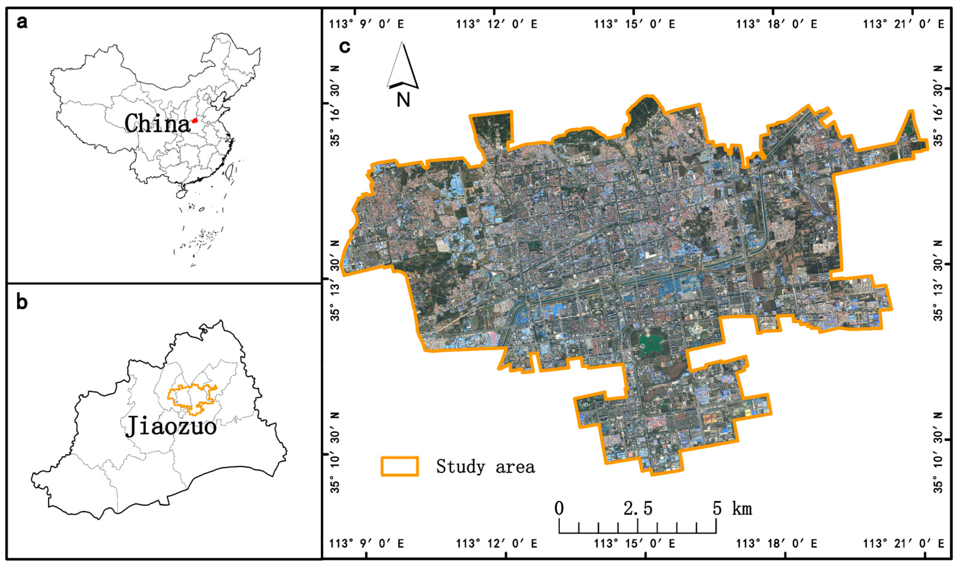
2.1. Study Scope: Jiaozuo, China

Jiaozuo city is a crucial city of the Central Plains Urban Agglomeration in China, located at 35°10′ N to 35°21′ N and 113°4′ E to 113°26′ E (Figure 1). Surrounded by Taihang Mountain and Huanghe River in the north and south, it contains 10 districts with an administrative area of approximately 4072 km². It is dominated by a tropical monsoon climate with heavy solar radiation in summer. The nominal annual average temperature is 14.9 °C and the nominal annual average precipitation is 551.6 mm (https://zh.m.wikipedia.org/, accessed on 11 September 2022). In the past few decades, Jiaozuo experienced rapid urban expansion, with an increase in the urbanization rate from 46.8% in 2010 to 63% in 2021 [23]. In our study, the core area of Jiaozuo city, which contains 850 urban planning and management units with a total administrative area of 120.3 square kilometers, was selected.

This study uses data from 2019 to 2020, a period typical of the urbanization development stage. The rapid urbanization process has significantly affected the urban thermal environment, and there is an urgent need to find ways to mitigate the UHI effect and provide new theories for urban planning and design.

2.2. Data Preparation

The Landsat 8 (path 119/row 42) remote sensing images for the four seasons used in this study were acquired from the USGS (http://earthexplorer.usgs.gov/ (accessed on 18 April 2019, 7 July 2019, 27 October 2019 and 31 January 2020)). The GF-2 image of Jiaozuo was prepared to extract land cover information (

Table 1. Information on remotely sensed data for Jiaozuo in this study.

Satellite	Path/Row	Resolution (m)	Period (Year–Month–Day)
			2019	2019	2019	2020
Landsat 8	119/42	30	18 April 2019	7 July 2019	27 October 2019	31 January 2020
GF-2	—	0.8	5 May 2019	25 September 2019	—	—

). In order to eliminate the effects of wind speed, surface humidity and solar radiation intensity, we pre-processed the images from remote sensing with atmospheric correction, radiometric calibration and image registration [24,25,26]. The administrative division was derived from the Jiaozuo Official Website (http://www.jiaozuo.gov.cn/ (accessed on 15 June 2019)).

2.3. Land Surface Temperature Retrieval

In this paper, we pick a cloud-free date in each season to extract the surface temperature to represent the spatial distribution of surface temperature in that season. The time between each two seasons is separated by three months. Referring to the study methods of Li and Peng, we used the LST of four dates, April 18, July 7, October 27 and January 31, to represent the four seasons, respectively [9,27]. Band 10 and band 11 in Landsat 8 remote sensing images are thermal infrared bands. The USGS discourages the use of the split-window algorithm (SW) to obtain the LST because of the instabilities in the participation of band 11 [28]. The radiation transport equation (RTE) algorithm is more accurate than single-channel (SC) algorithm and SW [29]. Thus, we extracted the LST using the RTE method. The calculation of this method used band 10 of Landsat 8 remote sensing images (1):

$$B_i\left(T_i\right)={\tau }_i\left(\theta \right)\left[{\epsilon }_i{B}_i\left(T_S\right)+\left(1-{\epsilon }_i\right)I_i^{\downarrow }\right]+I_i^{\uparrow }$$

(1)

In the above equation, $T_i$ is the lightness temperature sensed by the sensor, while $B_i\left(T_i\right)$ is the radiance of $T_i$. The correction parameters for the TIRS sensor can be obtained on the USGS website. ${\epsilon }_i$ represents the land surface emissivity for channel I, and $B_i\left(T_s\right)$ is the degree of surface radiance. $\theta$ shows the sensor angle, ${\tau }_i\left(\theta \right)$ is the transparency of the atmosphere, in which i is the number of the sensor channel. $I_i^{\uparrow }$ and $I_i^{\downarrow }$ are known as the uplink radiance and downlink radiance of the atmosphere, respectively. The atmospheric correction parameters for calculations $I_i^{\uparrow }$, $I_i^{\downarrow }$ and ${\tau }_i\left(\theta \right)$ can be downloaded from the NASA website. $B_i\left(T_{\mathrm{s}}\right)$ is the radiation intensity of a blackbody in the same apparent heat temperature in band 9, and the equation is calculated as follows:

$$B_i\left(T_s\right)=2h{c}^2/\left({\lambda }_i^5\ast \left(exp\left(hc/{\lambda }_{i}k{T}_s\right)-1\right)\right)$$

(2)

In Equation (2), $T_s$ means the LST, c is the velocity of light, ${\lambda }_i$ is the active wavelength of frequency band i, k is the Boltzmann constant and h is the Planck constant. ${\lambda }_i$ is calculated as follows (4):

$${\lambda }_i=\frac{{{\displaystyle \int }}_{{\lambda }_{1,i}}^{{\lambda }_{2,i}}{f}_i\left(\lambda \right)\lambda d\lambda }{{{\displaystyle \int }}_{{\lambda }_{1,i}}^{{\lambda }_{2,i}}{f}_i\left(\lambda \right)d\lambda }$$

(3)

In Equation (3), $f_i\left(\lambda \right)$ is the optical response function. ${\lambda }_{1,i}$ and ${\lambda }_{2,i}$ are the underside and upside border of $f_i\left(\lambda \right)$. Based on the converse function of Planck’s formula, the real LST ($T_s$) can be calculated as follows:

$$T_s=\frac{C_1}{{\lambda }_i\ln \left(\frac{C_2}{{\lambda }_i^5\left(B_i\left(T_i\right)-I_i^{\uparrow }-{\tau }_i\left(1-{\epsilon }_i\right)I_i^{\downarrow }\right)/{\tau }_i{\epsilon }_i}+1\right)}$$

(4)

The $C_1$ and $C_2$ in the above equations are constants, which can be checked in the MTL file in the image source file.

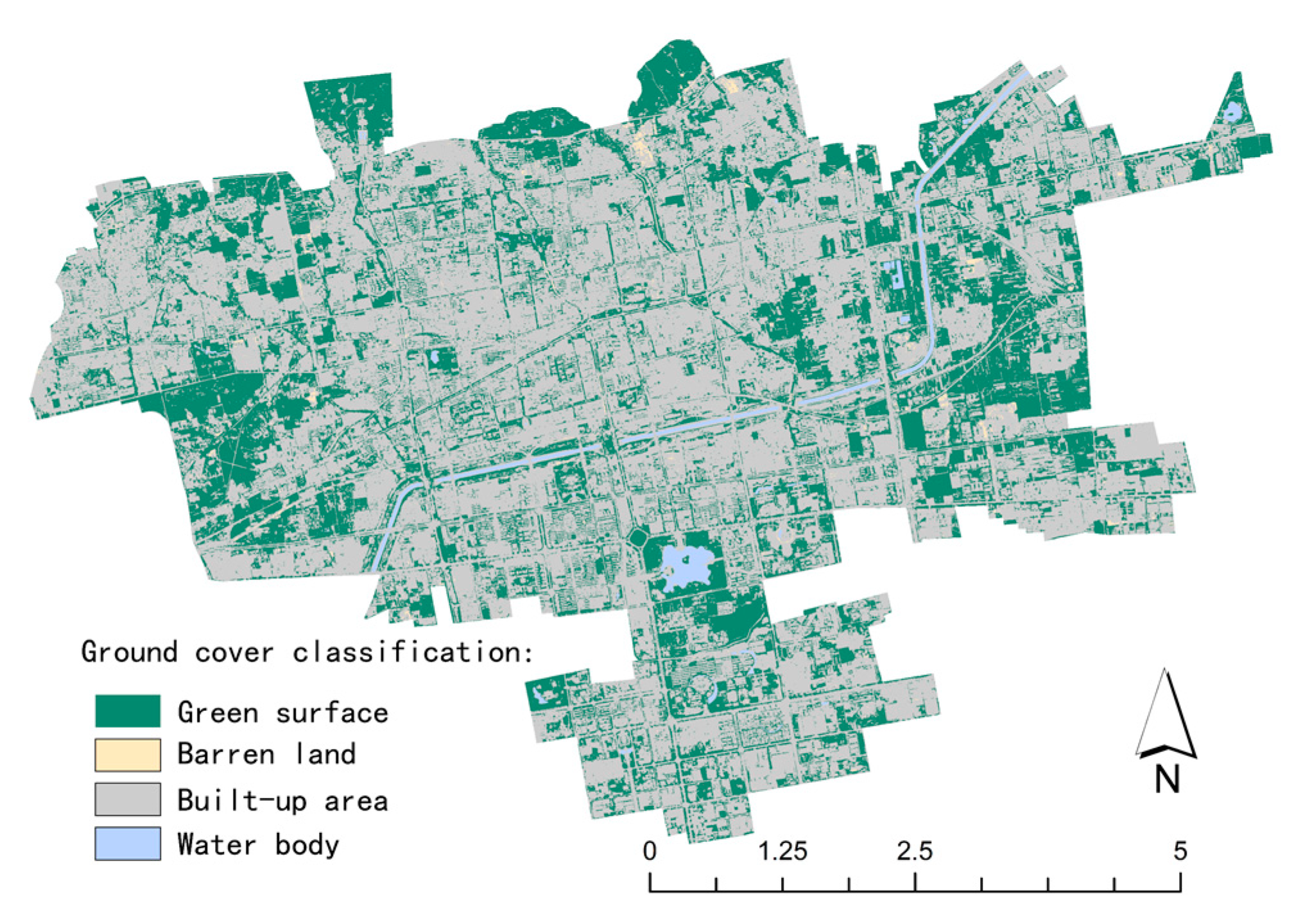
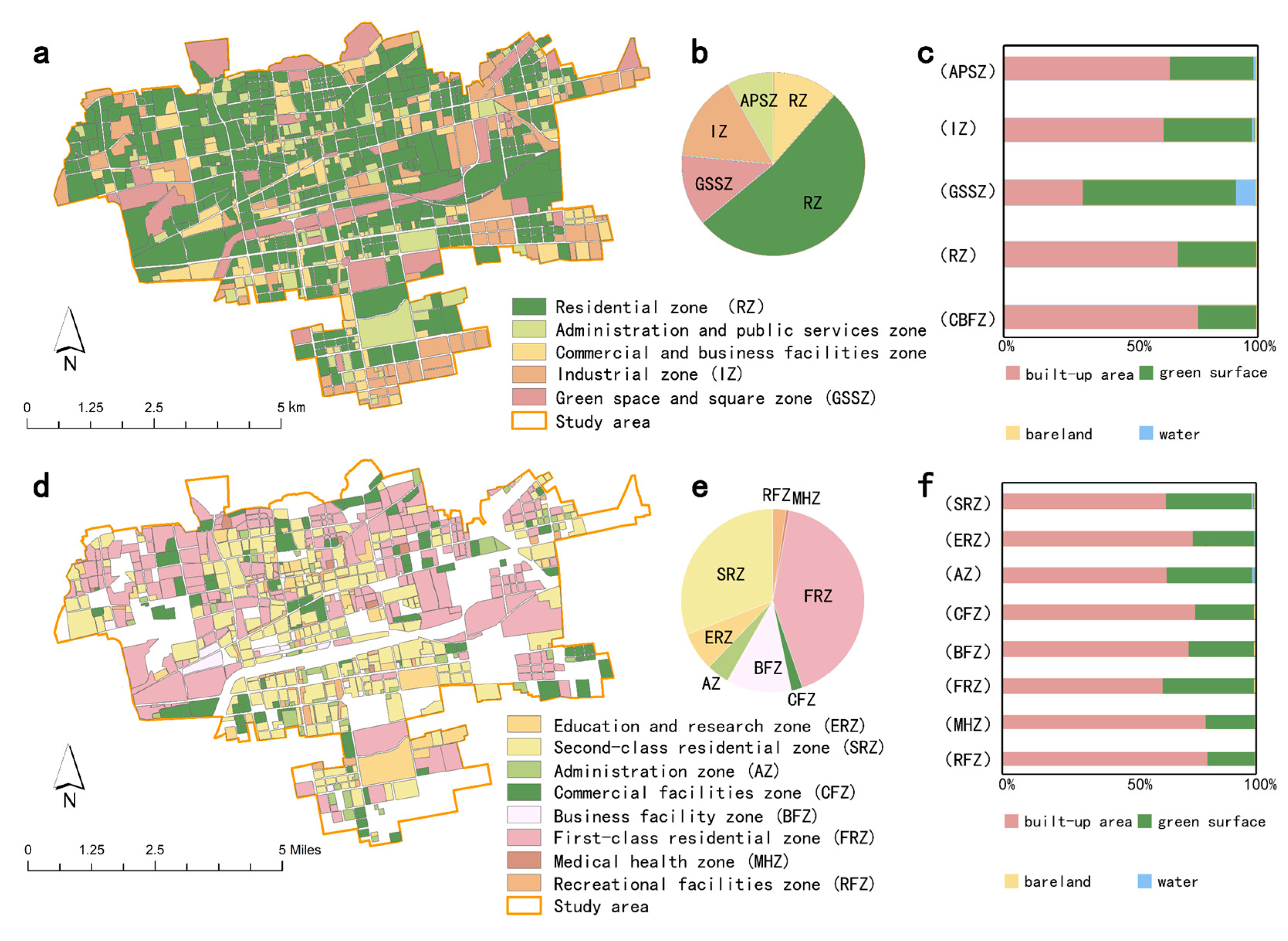
2.4. Interpretation of Land Cover and Land Use Types

According to related studies, the highest vegetation biomass season is summer; thus, the GF-2 remote images used in our research were captured in summer, which can fully reflect the urban vegetation information and be helpful for the classification of land cover. The classification of land cover types was performed in ENVI software [30]. Land cover was categorized into four kinds: green surface, barren land, built-up areas and water bodies (Figure 2). Green space is the area marked by vegetation cover, including woodland, shrubland and herbaceous vegetation. Water bodies include lakes, rivers and ponds. Built-up areas include impervious surfaces such as roads, buildings and squares. The land cover classification was assessed for accuracy; the overall accuracy rate was 98.7552% and the kappa coefficient was equal to 0.9819, satisfying the accuracy assessment requirements [31].

In addition, the administrative division of Jiaozuo was used to divide the land use types manually. In previous studies, some scholars argue that roadways not only play a role in cities to separate different use spaces but also can prevent heat exchange between adjacent urban spaces [32]. Therefore, our study not only uses the land use division of urban planning but also uses the urban roads as land use edges. Finally, the 850 planning management units were classified separately into five and eight categories (Figure 3a,d). The first category of land use was classified into five categories, namely residential zone (RZ), industrial zone (IZ), administration and public services zone (APSZ), commercial and business facility zone (CBFZ) and green space and square zone (GSSZ). The second category of land was separated into eight categories, namely first-class residential zone (FRZ), second-class residential zone (SRZ), administration zone (AZ), education and research zone (ERZ), medical health zone (MHZ), commercial facility zone (CFZ), business facility zone (BFZ) and recreational facility zone (RFZ).

The classification of land use types and their proportional areas are shown in Figure 3 and

Table 2. Statistics of sample size and regional information.

Land Use Types		Number of Samples	Area (m2)
IZ		94	16,007,740
GSSZ		50	13,032,007
RZ	FRZ	218	31,412,640
	SRZ	212	23,257,550
APSZ	AZ	56	2,993,336
	ERZ	35	5,148,938
	MHZ	10	437,956
CBFZ	CFZ	84	8,639,423
	BFZ	28	1,495,290
	RFZ	57	1,762,251

. The area of each planning management unit ranges from 8.6 to 54.9 km² in the first category and 0.43 to 31.4 km² in the second category. The first-category land use types, ranked from highest to lowest by area size, were RZ, IZ, GSSZ, CBFZ and APSZ (Figure 3a). The second-category land use types, ranked from highest to lowest by area size, were FRZ, SRZ, CFZ, ERZ, AZ, RFZ, BFZ and MHZ. The composition of land cover in each land use type is shown in Figure 3.

2.5. Landscape Metrics

In research on ecological processes and spatial patterns, the method of quantifying spatial heterogeneity is an important issue [33]. Landscape metrics are one of the most helpful methods for quantifying the spatial structure of an urban zone [34]. In addition, landscape composition and configuration have a driving effect on LST [35].

In this study, the potential drivers of LST included area and edge metrics (AREA, TA, PLAND), shape metrics (SHAPE, PAFRAC, FRACT), core metrics (TCA, CPLAND, DCAD), aggregation metrics (IJI, AI, NP, PD) and diversity metrics (SHDI, SIDI), a total of 15 metrics. Area and edge metrics include landscape area, patch area and the proportion of landscape area occupied by the same kind of patch. The shape metric describes the complexity of the shape, where the values of each of the three metrics increase unrestrictedly with the trait becoming irregular. Aggregation metrics indicate the degree of aggregation. The IJI and AI metrics increase with the aggregation of patches, and the values of these two metrics are maximum when the same type of plate is summed as one patch, but at the same time, the values of NP and PD will decrease. Diversity metrics describe the richness of patch species in the landscape. SHDI and SIDI use different approaches to complete this statistical process [36]. They were calculated for each planning management unit using Fragstats 4.2 (Kevin Mcgarigal&Eduard Ene, Amherst, MA, USA) software [37].

For different urban land uses, we analyzed the LST drivers. With the multiple linear regression method, we extracted the trends of LST with landscape structure index in different land use types. Jamieson demonstrated that the NRMSE value of the multiple linear regression model is less than 10% with high accuracy [38]. We explain the relationship between each variable and the trend of surface temperature change by determination coefficient (R²) in the multiple linear regression results.

3. Results

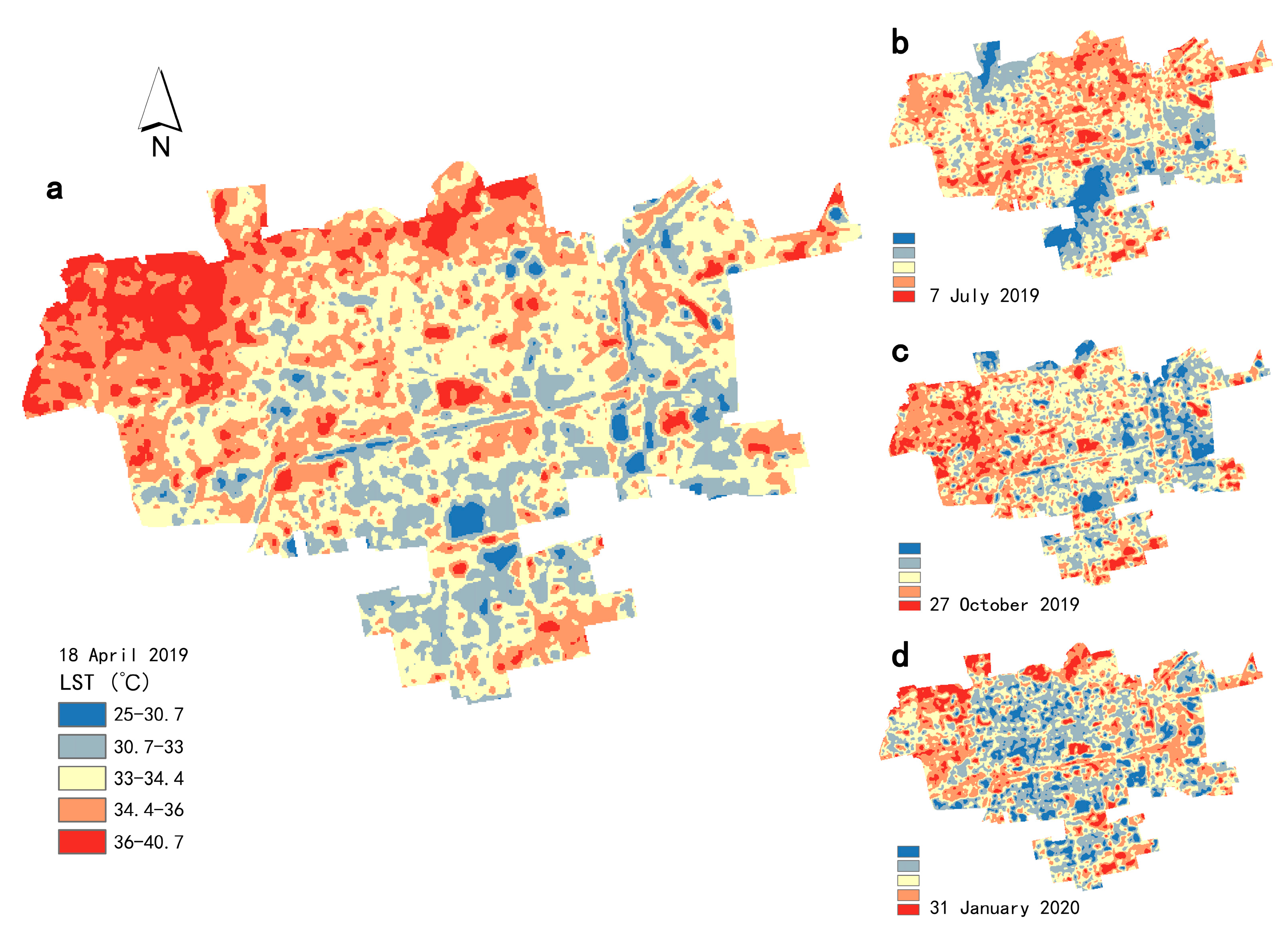
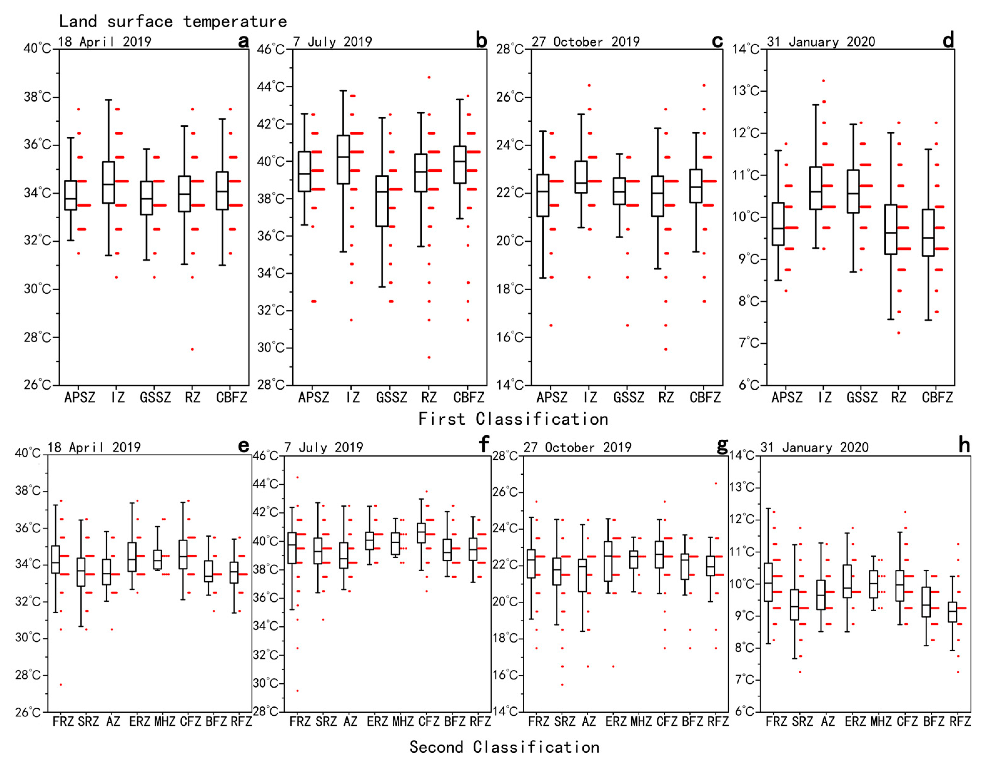
3.1. Spatiotemporal Pattern of LST

Based on the LST map acquired from Landsat 8 images (Figure 4), the minimum LST in our research area is 4.7 °C and the maximum LST is 50 °C in 2019–2020. The average LSTs in the four months were 32.8 °C, 39.7 °C, 21.7 °C and 10.3 °C, with an average difference of 10 °C between adjacent seasons.

Areas of high urban surface temperature appear to be clustered in surrounding areas; in addition, the city center area shows a significant cooling effect in winter. The distribution of high-LST areas in April and July is unbalanced in the city. High-LST areas in April are clustered in the northwestern part of the city; in July, high-LST areas were distributed in the west part of the city and a few were scattered in the south part of the city area. In October, the LST in the city central area was greater than that in the surrounding areas, while in January, the LST was lower in the city central area than in the surrounding areas. Experiments have proven that the areas of the highest urban surface temperatures are not in the geographic city center and that the two are not identical in space.

There are high variations in LST between different land use types, and these variations vary with seasons. Figure 5 shows that the standard deviation of LST for each land use type was the maximum in July and the minimum in January. The LST of the industrial zone has the maximum standard deviation in the months of April and July. The residential zone has the maximum standard deviation in January. The first-class residential zone LST has a high standard deviation in April and mid-July, and the gaps between the highest and lowest temperatures are 5.96 °C and 6.90 °C, respectively.

Comparing the LST of different land use types, the average LST of the industrial zone was found to be higher than that of other site types in all four seasons. The LST of the green space and square zone experienced the maximum variation among four seasons. In addition, the LST of the green space and square zone was minimum in the season with hot weather and maximum in the season of cold compared to other land use types. In the category of administration and public services zone, the LST of the administration zone was lower than that of the education and research zone and medical health zone. The LST of the second-class residential zone was lower than that of the first-class residential zone. The second-class residential zone is mostly distributed in the city center, while the first-class residential zone is mostly distributed at the edge of the city. Considering the spatial distribution of the two types of land use, the first-class residential zone in the urban suburbs has a higher LST than the second-class residential zone in the urban center.

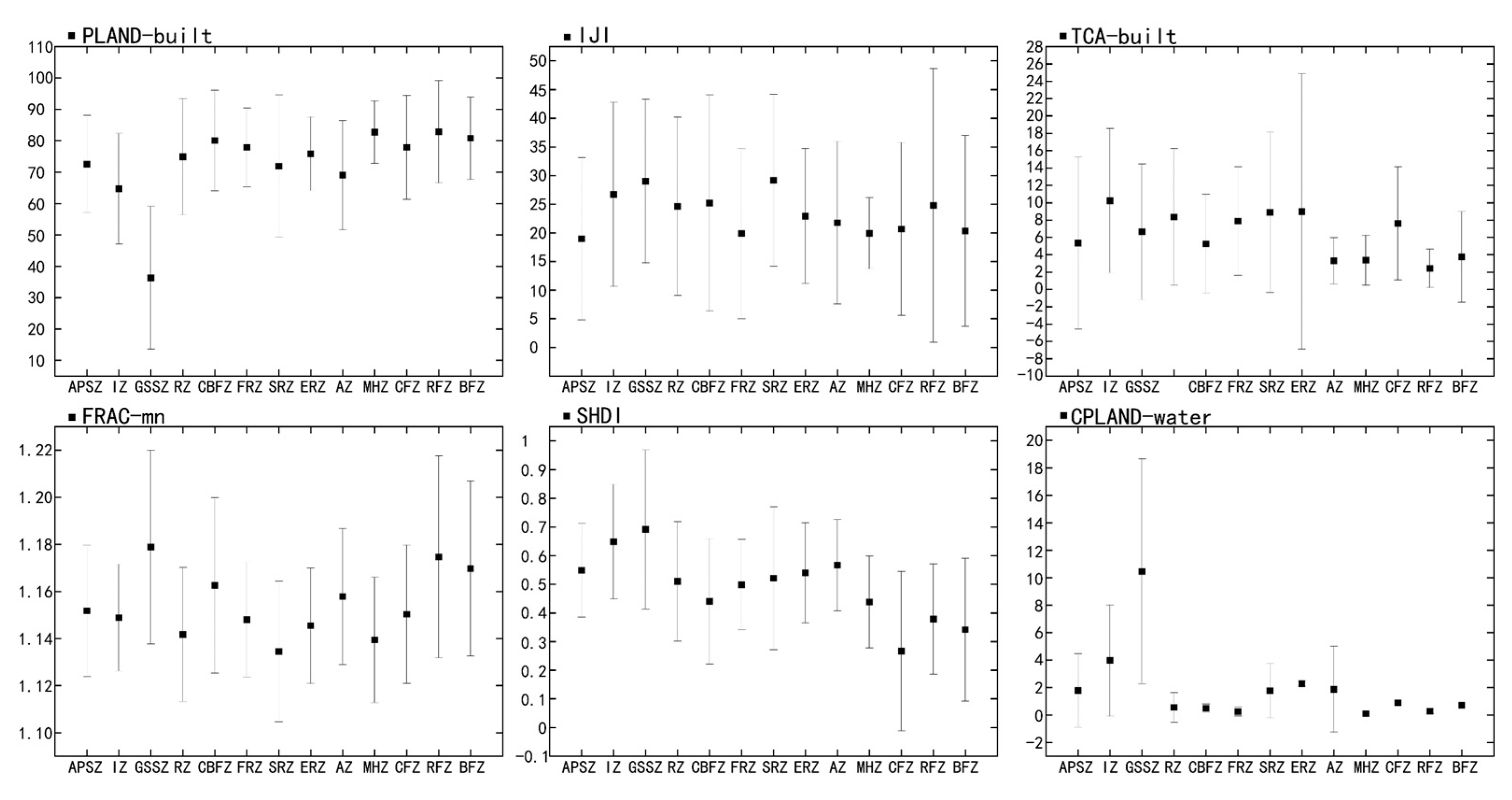
3.2. Spatial Changes of Landscape Metrics

Using statistics on the landscape metrics, the difference in landscape patterns between land use types was observed (Figure 6). In particular, significant landscape structure features were observed in the green space and square zone, residential zone and industrial zone. In the green space and square zone, the intensity of urbanization is low, compared to the high proportion of green spaces and water bodies, and there is a low degree of landscape fragmentation and a high richness of patches. Compared with the first-class residential zone, the second-class residential zone has a larger landscape area, lower urbanization intensity, greater landscape fragmentation and high aggregation. Compared with other land use types, the industrial zone has a high total core area for impermeable patches. However, the urbanization intensity in the industrial zone is lower than that in most of the land use types.

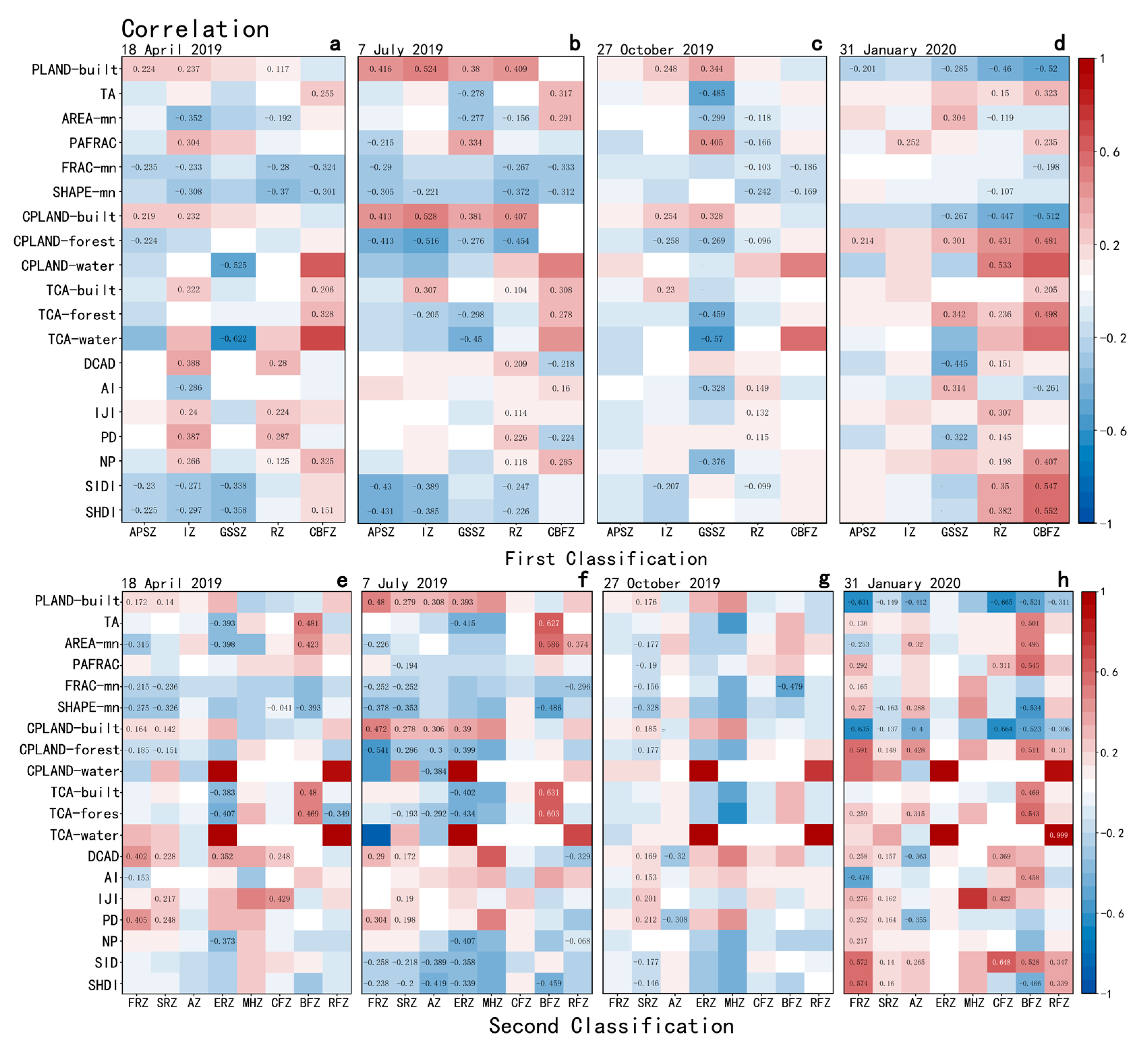
3.3. Correlation between LST and Landscape Pattern

On the first land use classification scale, LST was significantly correlated with urbanization intensity and green surface coverage for each urban land use type (Figure 7). A remarkable positive association was observed between LST and the percentage intensity of urbanization in April, July and October, and in January it became negatively correlated. SIDI, SHDI and CLAND-forest were correlated negatively with LST in April, July and October and positively correlated in January. FRAC-mn, SHAPE-mn and TCA-water were all correlated negatively with LST, while TCA-built and IJI were positively correlated. SHDI, SIDI and CPLAND had consistent correlations for LST. NP and PD have a negative impact on green space and square zone LST in October and January while they have a positive impact on LST of other land use types. Compared with AREA-mn, PAFRAC, DCAD and AI, the results show that an increase in landscape fragmentation of industrial and green space and square zones leads to an increase in LST.

Compared to land use types of the first category, the second-category land use types show a complex correlation with LST. Land use types from the same first-category land use showed similar correlations between the landscape structure and LST; they have similar negative or positive effects but differ in value.

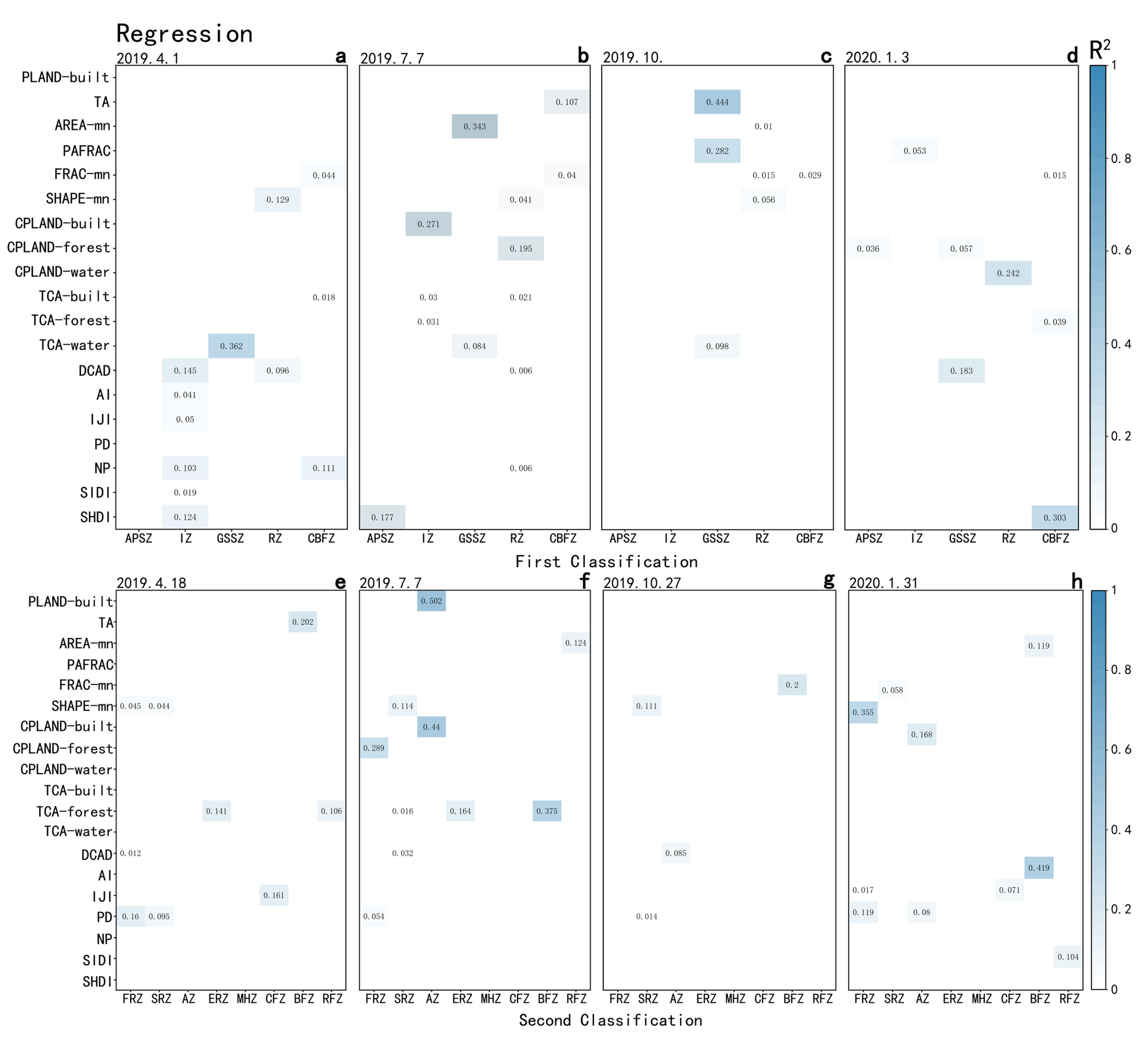
3.4. Relative Importance of Landscape Driving Forces

Drivers of LST exhibit complex variation across seasons and land use types (Figure 8). LST of green space and square zone can be well explained by TCA-water (36.2%), AREA-mn (34.3%), TA (44.4%) and DCAD (18.3%). LST of the green space and square zone is mainly influenced by the area and the percentage of water bodies. DCAD (14.5%) and CPLAND-built (27.1%) act as the main drivers of LST for the industrial zone in April and October. The high percentage of impervious surface is the primary source of high LST in the industrial zone. SHAPE-mn and CPLAND play an important role in explaining the LST of the residential zone in April, July and January. Residential zones with high landscape fragmentation or high aggregation of green surface and water patches show lower LST. SHDI can well explain the LST of the administration and public services zone (17.7%) and commercial and business facility zone (30.3%) in July and January. In administration and public services zones and commercial and business facility zones that lack green space or water bodies, an appropriate amount of green surface and water body patches can well reduce the surface temperature.

The percentage of impervious surfaces and the degree of fragmentation can well explain the LST of the administration zone. PLANND-built (50.2%) and CPLAND-built (44%) can well explain the change in LST in the administration zone in July, while CPLAND-forest plays an important role in January (16.8%). TCA-forest has the greatest impact on the LST of the education and research zone in April (14.3%) and July (16.4%). The LST of the education and research zone can be effectively reduced by increasing the area of core green surface patches. The main drivers of landscape structure in first-class residential zone are SHAPE-mn and PD. CPLAND-forest (35.5%) and CPLAND-built (28.9%) can well explain the LST of the second-class residential zone in July and January; PD was the most important driver in January (16%). The increase in fragmentation in impervious surfaces and the decrease in fragmentation in green surface patches will reduce the LST of the second-class residential zone. Furthermore, the impact on the LST of the second-class residential zone is greater than that of the first-class residential zone. In different seasons, TA (20.2%), CPLAND-forest (37.5%), CPLAND-built (37.5%) and AI (41.9%) contribute to the LST of the business facility zone. CPLAND-forest (10.6%), AREA-mn (12.4%) and SIDI (10.4%) contributed to the LST of the recreational facility zone in April, July and January. With the decrease in landscape area and the increase in fragmentation, the LST of the business facility zone decreases, while the LST of the recreational facility zone increases.

4. Discussion

4.1. Relationships between Anthropogenic Heat and LST

Previous studies have demonstrated that as the intensity of built-up land varies in different parts of the urban area, it leads to changes in the radiative surface [39]. In our study, the spatial distribution of surface temperature in urban areas is further described. At the spatial scale of the city, high-LST areas in the built-up area of Jiaozuo city are distributed in surrounding areas of the city in most seasons, with low numbers of high-LST patches in the city center area. Similar situations have emerged in previous studies. Sun found that the high-LST areas in Beijing clustered in the northwestern part of the city, not in the central part of the city [40]. Meanwhile, it was revealed that obvious differences in LST existed in different urban land use types. Some research suggests that landscape heterogeneity is one of the causes of this phenomenon [41,42]. Yue believes that the factors affecting urban LST can be divided into three aspects: urbanization intensity, landscape structure and human activities [4]. In our experiments, we also found a positive correlation between urbanization intensity and each urban land use type, and we try to provide some theoretical basis for solving the UHI effect by explaining the effect of landscape structure on different land use types.

The impact of heat emissions from human activities on LST is frequently difficult to calculate. Changes in population density and per capita energy use can affect urban consumption of energy forms such as electricity and gas, resulting in anthropogenic heat emissions [43]. The results of Chapman’s study revealed that anthropogenic heat emissions could lead to a 4 °C increase in LST; such human activities include transportation, building energy and human metabolism [44]. It is not sufficient to explain the urban-scale LST distribution by a small amount of human activity alone, but it proves that the impact of human activities on LST cannot be ignored. Previous experimental results reveal a spatial pattern of the anthropogenic exothermic activity always associated with the industrial zone [45], and the LST of the industrial zone tends to be higher than that of other land use types [40,46,47].

The warming trend appears greater in peri-urban areas compared to urban centers. The spatial distribution of newly expanded high-LST areas agrees with that of the industrial zone [48,49]; we have similar experimental results. At the same time, considering the effects of changes in solar radiation intensity and changes in human activity intensity on LST in different seasons, comparisons were made between each of the four seasons. From the experimental results, it is found that the surface temperature of commercial and park land is similar to that of industrial land in July and January. Kato and Du et al. demonstrated that heat rejection from human activities is maximum in summer and winter and minimum in spring and autumn [50]. This is to some extent corroborated by our experimental results. The commercial and business facility zone in our study area has a high percentage of commercial facility zone with a high percentage of imperviousness, and it is also subject to more heat emissions from human activities in the summer, therefore suffering high LST. Both the commercial and business facility zone and the industrial zone are distributed in the peripheral areas of the city, resulting in the clustering of high-LST areas in the periphery. The percentage of green surface was correlated negatively with LST in January, implying that the green surface has a warming effect in the low-temperature season, and it is subject to higher anthropogenic heat emissions, which result in higher LST in the green space and square zone in winter. Our results showed that the administration and public services zone and second-class residential zone had lower LST. Similar findings were obtained in the study of Zhao and were attributed to the high greening rate [51].

4.2. Relationships between Landscape Structure and LST

The results of our study prove that both urban land use types and urban landscape structure have explanatory effects on LST, and this correlation has seasonal differences. Previous studies have generally concluded that the UHI effect can be effectively mitigated by controlling land cover types and adjusting urban landscape patterns [52]. In urban areas, hybrid land cover types have lower surface temperatures compared to a single impervious surface [9]. This phenomenon may be attributed to the fact that the complex patch morphology favors heat transfer [3,53,54]. We obtained similar results in this study. Moreover, by comparing the LSTs in different periods, we concluded that the explanation effect of landscape structure on LST has seasonal variability. In addition, large differences also occur between different land use types in the same season. Rinner concluded that the areas of the industrial zone and the green space and square zone have an opposite contribution to driving surface temperature [47]. Our study again proves these conclusions. On this basis, the results of our experiments demonstrate that the reason for the difference between the industrial zone and the green and square zone is the extreme imbalance between the percentages of impervious and green surfaces in the landscape.

As shown in Figure 5a,b, the maximum standard deviation of the surface temperature of industrial land occurs during April and July, the period of higher air temperature. The possible explanation for this result is that different types of industrial zones have different implications for LST; significant differences can be found between the LSTs of heavy industry and high-tech industries [55]. In addition, there are more heat sources in the high-temperature season compared to the low-temperature season, which will contribute to a greater difference in LST [56,57,58]. Peng’s study demonstrates a significant decrease in LST in landscapes with a proportion of green space above 70%, and a strong correlation between landscape pattern index and LST emerges in landscapes with a proportion of green space above 70% [59]. For green space and square zone, we reached a similar conclusion. Furthermore, we found that in the actual urban planning, only the green surface ratio of the green space and square zone is within this range (Figure 3c).

Our results show that the surface temperature of the first-class residential zone is higher than that of the second-class residential zone (Figure 5). Similar results were observed in a previous study showing that the LST of a low-architecture zone is higher than that of high-building areas [60]. Such a finding can be explained by the varying three-dimensional structure of the architecture. Gage and Yin’s results also suggest that architectural structure plays a more significant role in LST than land cover in the residential zone [61]. Lan’s study demonstrated that LST received increased influence from the three-dimensional structure of the architecture as the architecture density and height increased [62]. Li believes that this phenomenon can be explained by aerodynamics [9]; buildings with taller floors have stronger aerodynamic conductivity to carry heat away from the surface. Giridharan and Magli attribute this to the masking effect of tall buildings, where the ground receives less radiation, resulting in lower surface temperatures [63,64]. However, it has been suggested that high-density high-rise buildings impede air circulation in urban areas [65,66], which leads to heat accumulation and a continuous increase in LST. This implies that high-rise buildings can reduce some LST, but this cooling effect decreases with increasing building density.

In terms of spatial location, we find that the second-class residential zone with lower LST is mainly distributed in the urban center area, while the first-class residential zone with higher LST is mainly located in the peripheral areas of the city. Compared with the UHI effect, which causes the high LST in the urban center area, the urban land use classification shows a greater explanatory effect on LST, and it has a masking effect on the spatial distribution of LST in urban areas caused by the UHI effect.

4.3. Planning Strategy Implication

In previous urban planning practices, urban planners often attempted to create a comfortable and cool environment by expanding the number of green spaces. With the rapid expansion of cities, land resources available for green space compete against other socio-economic benefits, making it difficult to carve out any other green space in urban areas. Many scholars suggest that the perspective should be changed and efforts of optimal spatial allocation should be made within the limited space. For example, changing the spatial connectivity and complexity of the city can significantly reduce the LST with no change in green space coverage [40]. In addition, the LSTs of different types of urban land use show significant differences. Therefore, urban planners should adapt different spatial allocation optimization methods for different types of urban land use. For example, increasing the proportion of water bodies in the green space and square zone can significantly reduce LST. Increasing the fragmentation of water bodies or green spaces and reducing the fragmentation of impervious surfaces in the industrial zone can reduce LST (Figure 9). In contrast to the industrial zone, the increase in the fragmentation of impervious surfaces and the decrease in fragmentation of green surface patches are conducive to reducing the LST of the second-class residential zone. The LST of second-class residential zone use is lower than that of first-class residential zone use, so we can also consider vertical urban development to avoid damage to urban green spaces as much as possible [60,67].

The Chinese government has issued various policies to mitigate UHIs as a climate problem, such as sponge cities, forest cities and climate-sensitive cities [68]. The implementation of the “Hundred Enterprises Retreating from the City” and “Green Shield” policies released by the Jiaozuo city government in November 2019 has played a significant role in reducing the urban heat island effect. Our study further provides effective theoretical and practical information for urban planners by showing how to minimize the UHI effect by changing the urban spatial structure when the proportion of green space in urban space is limited.

4.4. Limitations and Suggested Future Research

We use urban planning units as our basic spatial units in our study; in comparison to a regular grid as the basic cell, irregular spatial cells may result in a loss of edge details in the raster image. However, there is no fixed unit of analysis for UHI studies, and the method we use is not a bad attempt to align with urban planning and design. These results are based on single-day LST for four months of one year, and sufficient images were not available to analyze the LST separately for daytime and nighttime comparisons during the day. A more accurate understanding of the variation of surface temperature over time in each urban site would be possible if we additionally compared and analyzed the daytime and nighttime surface temperatures in each season, as Zhou did [57].Meanwhile, we used four Landsat 8 images with 30 m resolution to extract the surface temperature, which has some limitations. In future studies, the average seasonal surface temperature can be used for research under good imaging conditions. The study conclusions are based on the supposition that urban roads isolate most of the heat exchange between adjacent areas. The relationship between LST and landscape structure is quantified on a per site area basis. However, the surface temperature of each site area will be influenced by the adjacent areas, which may affect the accuracy of our study.

5. Conclusions

Rapid urbanization has changed the surface structure, and land use types and landscape structure have profound impacts on the spatial variation of LST. With high-intensity human activities, built-up areas always concentrate sophisticated land use types. Among existing studies, numerous studies focus on the relationship between urban–rural gradient, urbanization intensity and surface temperature; however, many research results are difficult to translate into practical urban construction strategies. We found that few investigations have been carried out on the relationship between land use types and LST. Land use in urban systems is very complex, and there are numerous elements that interact with the urban thermal environment. A comprehensive understanding of the current status of land use in urban space and studying the relationship between landscape structure and LST from multiple perspectives are beneficial for understanding the driving factors and characteristics of LST in highly urbanized areas. In this research, we analyzed the impacts of urban landscape structure on LST by a regression method based on the example of Jiaozhou, China. Particularly, we investigated the effects of landscape metrics in different land use types on LST to determine the main driving factors of LST. The results of this study indicate that the spatial distribution of the industrial zone in the city can well explain the distribution of high-LST areas. Green space and square zones have the capacity to raise the surface temperature in winter. By comparing the correlations and regression analysis between the landscape metrics and LST under different land use types, we found that an increased landscape fragmentation will lead to an increase in LST for the industrial zone and green space and square zone but will lead to a decrease in LST for the residential zone. The LST of first-class residential zone is higher than that of the second-class residential area; in addition, the landscape metrics in the first-class residential zone show less of an ability to explain the LST. This finding demonstrates that different LSTs of the residential zone can be explained by the 3D structure of buildings. LST can be reduced through old city renovation.

References

1. Li, W.; Bai, Y.; Chen, Q.; He, K.; Ji, X.; Han, C. Discrepant Impacts of Land Use and Land Cover on Urban Heat Islands: A Case Study of Shanghai, China. Ecol. Indicat. 2014, 47, 171–178. [Google Scholar] [CrossRef]
2. National Bureau of Statistics of China. Available online: http://www.stats.gov.cn/was5/web/search?channelid=288041&andsen=%E5%9F%8E%E9%95%87%E5%8C%96%E7%8E%87 (accessed on 2 September 2022).
3. Li, W.; Cao, Q.; Lang, K.; Wu, J. Linking Potential Heat Source and Sink to Urban Heat Island: Heterogeneous Effects of Landscape Pattern on Land Surface Temperature. Sci. Total Environ. 2017, 586, 457–465. [Google Scholar] [CrossRef]
4. Oke, T.R. The Energetic Basis of the Urban Heat Island. Q. J. Royal Met. Soc. 1982, 108, 5502. [Google Scholar] [CrossRef]
5. Zhang, Y.; Middel, A.; Turner, B.L. Evaluating the Effect of 3D Urban Form on Neighborhood Land Surface Temperature Using Google Street View and Geographically Weighted Regression. Landscape Ecol 2019, 34, 681–697. [Google Scholar] [CrossRef]
6. Gober, P.; Brazel, A.; Quay, R.; Myint, S.; Grossman-Clarke, S.; Miller, A.; Rossi, S. Using Watered Landscapes to Manipulate Urban Heat Island Effects: How Much Water Will It Take to Cool Phoenix? J. Am. Plann. Assoc. 2009, 76, 109–121. [Google Scholar] [CrossRef]
7. Impact of Regional Climate Change on Human Health | Nature. Available online: https://www.nature.com/articles/nature04188 (accessed on 27 March 2022).
8. Dissanayake, D.; Morimoto, T.; Murayama, Y.; Ranagalage, M. Impact of Landscape Structure on the Variation of Land Surface Temperature in Sub-Saharan Region: A Case Study of Addis Ababa Using Landsat Data (1986–2016). Sustainability 2019, 11, 2257. [Google Scholar] [CrossRef]
9. Li, J.; Song, C.; Cao, L.; Zhu, F.; Meng, X.; Wu, J. Impacts of Landscape Structure on Surface Urban Heat Islands: A Case Study of Shanghai, China. Remote Sens. Environ. 2011, 115, 3249–3263. [Google Scholar] [CrossRef]
10. Imhoff, M.L.; Zhang, P.; Wolfe, R.E.; Bounoua, L. Remote Sensing of the Urban Heat Island Effect across Biomes in the Continental USA. Remote Sens. Environ. 2010, 114, 504–513. [Google Scholar] [CrossRef]
11. Chow, W.T.L.; Roth, M. Temporal Dynamics of the Urban Heat Island of Singapore. Int. J. Climatol. 2006, 26, 2243–2260. [Google Scholar] [CrossRef]
12. Göttsche, F.-M.; Olesen, F.-S.; Trigo, I.; Bork-Unkelbach, A.; Martin, M. Long Term Validation of Land Surface Temperature Retrieved from MSG/SEVIRI with Continuous in-Situ Measurements in Africa. Remote Sens. 2016, 8, 410. [Google Scholar] [CrossRef] [Green Version]
13. Guo, G.; Wu, Z.; Xiao, R.; Chen, Y.; Liu, X.; Zhang, X. Impacts of Urban Biophysical Composition on Land Surface Temperature in Urban Heat Island Clusters. Landsc. Urban Plann. 2015, 135, 7. [Google Scholar] [CrossRef]
14. Hu, D.; Meng, Q.; Zhang, L.; Zhang, Y. Spatial Quantitative Analysis of the Potential Driving Factors of Land Surface Temperature in Different “Centers” of Polycentric Cities: A Case Study in Tianjin, China. Sci. Total Environ. 2020, 706, 135244. [Google Scholar] [CrossRef]
15. Jia, W.; Zhao, S. Trends and Drivers of Land Surface Temperature along the Urban-Rural Gradients in the Largest Urban Agglomeration of China. Sci. Total Environ. 2020, 711, 134579. [Google Scholar] [CrossRef] [PubMed]
16. Yuan, S.; Xia, H.; Yang, L. How Changing Grain Size Affects the Land Surface Temperature Pattern in Rapidly Urbanizing Area: A Case Study of the Central Urban Districts of Hangzhou City, China. Environ. Sci. Pollut. Res. 2021, 28, 40060–40074. [Google Scholar] [CrossRef] [PubMed]
17. Zhao, X.F.; Deng, L.; Wang, H.N.; Hua, L.Z.; Chen, F. Landscape Classifications for Landscape Metrics-Based Assessment of Urban Heat Island: A Comparative Study. IOP Conf. Ser.: Earth Environ. Sci. 2014, 17, 012155. [Google Scholar] [CrossRef]
18. Bokaie, M.; Zarkesh, M.K.; Arasteh, P.D.; Hosseini, A. Assessment of Urban Heat Island Based on the Relationship between Land Surface Temperature and Land Use/Land Cover in Tehran. Sustain. Cities Soc. 2016, 23, 94–104. [Google Scholar] [CrossRef]
19. Coseo, P.; Larsen, L. How Factors of Land Use/Land Cover, Building Configuration, and Adjacent Heat Sources and Sinks Explain Urban Heat Islands in Chicago. Landsc. Urban Plann. 2014, 125, 117–129. [Google Scholar] [CrossRef]
20. Wang, C.; Myint, S.; Wang, Z.; Song, J. Spatio-Temporal Modeling of the Urban Heat Island in the Phoenix Metropolitan Area: Land Use Change Implications. Remote Sens. 2016, 8, 185. [Google Scholar] [CrossRef]
21. Xie, L.T.; Cai, G.Y. Impact of Land Cover Types and Components on Urban Heat; Zhou, G., Kang, C., Eds.; International Conference on Intelligent Earth Observing and Applications: Guilin, China, 2015; p. 98080S. [Google Scholar]
22. Zipper, S.C.; Schatz, J.; Singh, A.; Kucharik, C.J.; Townsend, P.A.; Loheide, S.P. Urban Heat Island Impacts on Plant Phenology: Intra-Urban Variability and Response to Land Cover. Environ. Res. Lett. 2016, 11, 054023. [Google Scholar] [CrossRef]
23. Jiaozuo City Bureau of Statistics Statistical Bulletin_Henan Provincial Bureau of Statistics. Available online: https://tjj.henan.gov.cn/2020/05-20/1501269.html (accessed on 2 September 2022).
24. Velasco-Forero, S.; Manian, V. Improving Hyperspectral Image Classification Using Spatial Preprocessing. IEEE Geosci. Remote Sensing Lett. 2009, 6, 297–301. [Google Scholar] [CrossRef]
25. Wemmert, C.; Puissant, A.; Forestier, G.; Gancarski, P. Multiresolution Remote Sensing Image Clustering. IEEE Geosci. Remote Sensing Lett. 2009, 6, 533–537. [Google Scholar] [CrossRef]
26. Ranagalage, M.; Estoque, R.; Zhang, X.; Murayama, Y. Spatial Changes of Urban Heat Island Formation in the Colombo District, Sri Lanka: Implications for Sustainability Planning. Sustainability 2018, 10, 1367. [Google Scholar] [CrossRef]
27. Peng, J.; Jia, J.; Liu, Y.; Li, H.; Wu, J. Seasonal Contrast of the Dominant Factors for Spatial Distribution of Land Surface Temperature in Urban Areas. Remote Sens. Environ. 2018, 215, 255–267. [Google Scholar] [CrossRef]
28. Wan, Z. MODIS Land Surface Temperature Products. ERI, University of California, Santa Barbara. 33. Available online: https://lpdaac.usgs.gov/documents/118/MOD11_User_Guide_V6.pdf (accessed on 12 August 2022).
29. Yu, Z.; Guo, X.; Jørgensen, G.; Vejre, H. How Can Urban Green Spaces Be Planned for Climate Adaptation in Subtropical Cities? Ecol. Indicat. 2017, 82, 152–162. [Google Scholar] [CrossRef]
30. Talukdar, S.; Singha, P.; Mahato, S.; Shahfahad; Pal, S.; Liou, Y.-A.; Rahman, A. Land-Use Land-Cover Classification by Machine Learning Classifiers for Satellite Observations—A Review. Remote Sens. 2020, 12, 1135. [Google Scholar] [CrossRef]
31. Rwanga, S.S.; Ndambuki, J.M. Accuracy Assessment of Land Use/Land Cover Classification Using Remote Sensing and GIS. IJG 2017, 08, 611–622. [Google Scholar] [CrossRef]
32. Effect of Urban Function and Landscape Structure on the Urban Heat Island Phenomenon in Beijing, China | SpringerLink. Available online: https://link.springer.com/article/10.1007/s11355-019-00388-5 (accessed on 28 March 2022).
33. Global Patterns of Dissolved N, P and Si in Large Rivers | SpringerLink. Available online: https://link.springer.com/article/10.1023/A:1024960007569 (accessed on 28 March 2022).
34. Uuemaa, E.; Antrop, M.; Roosaare, J.; Marja, R.; Mander, Ü. Landscape Metrics and Indices: An Overview of Their Use in Landscape Research. Liv. Rev. Landsc. Res. 2009, 3, 2009-1. [Google Scholar] [CrossRef]
35. Peng, J.; Wang, Y.; Zhang, Y.; Wu, J.; Li, W.; Li, Y. Evaluating the Effectiveness of Landscape Metrics in Quantifying Spatial Patterns. Ecol. Indicat. 2010, 10, 217–223. [Google Scholar] [CrossRef]
36. Cardille, J.A.; Turner, M.G. Understanding Landscape Metrics. In Learning Landscape Ecology; Gergel, S.E., Turner, M.G., Eds.; Springer New York: New York, NY, USA, 2017; pp. 45–63. ISBN 978-1-4939-6372-0. [Google Scholar]
37. Kupfer, J.A. Landscape Ecology and Biogeography: Rethinking Landscape Metrics in a Post-FRAGSTATS Landscape. Progr. Phys. Geogr. Earth Environ. 2012, 36, 400–420. [Google Scholar] [CrossRef]
38. Jamieson, P.D.; Porter, J.R.; Wilson, D.R. A Test of the Computer Simulation Model ARCWHEAT1 on Wheat Crops Grown in New Zealand. Field Crops Res. 1991, 27, 337–350. [Google Scholar] [CrossRef]
39. Mallick, J.; Kant, Y.; Bharath, B.D. Estimation of Land Surface Temperature over Delhi Using Landsat-7 ETM+. J. Ind. Geophys. Union 2008, 12, 131–140. [Google Scholar]
40. Sun, R.; Lü, Y.; Chen, L.; Yang, L.; Chen, A. Assessing the Stability of Annual Temperatures for Different Urban Functional Zones. Build. Environ. 2013, 65, 90–98. [Google Scholar] [CrossRef]
41. Urban Heat Islands and Landscape Heterogeneity: Linking Spatiotemporal Variations in Surface Temperatures to Land-Cover and Socioeconomic Patterns | SpringerLink. Available online: https://link.springer.com/article/10.1007/s10980-009-9402-4 (accessed on 28 March 2022).
42. Seasonal Variations in the Relationship between Landscape Pattern and Land Surface Temperature in Indianapolis, USA | SpringerLink. Available online: https://link.springer.com/article/10.1007/s10661-007-9979-5 (accessed on 28 March 2022).
43. Kardinal Jusuf, S.; Wong, N.H.; Hagen, E.; Anggoro, R.; Hong, Y. The Influence of Land Use on the Urban Heat Island in Singapore. Habitat Int. 2007, 31, 232–242. [Google Scholar] [CrossRef]
44. Chapman, S.; Watson, J.E.M.; McAlpine, C.A. Large Seasonal and Diurnal Anthropogenic Heat Flux across Four Australian Cities. JSHESS 2016, 66, 342–360. [Google Scholar] [CrossRef]
45. Xiong, Y.; Huang, S.; Chen, F.; Ye, H.; Wang, C.; Zhu, C. The Impacts of Rapid Urbanization on the Thermal Environment: A Remote Sensing Study of Guangzhou, South China. Remote Sens. 2012, 4, 2033–2056. [Google Scholar] [CrossRef]
46. Assessing Spatial Pattern of Urban Thermal Environment in Shanghai, China | SpringerLink. Available online: https://link.springer.com/article/10.1007/s00477-012-0638-1 (accessed on 28 March 2022).
47. Rinner, C.; Hussain, M. Toronto’s Urban Heat Island—Exploring the Relationship between Land Use and Surface Temperature. Remote Sens. 2011, 3, 1251–1265. [Google Scholar] [CrossRef]
48. Yue, W.; Qiu, S.; Xu, H.; Xu, L.; Zhang, L. Polycentric Urban Development and Urban Thermal Environment: A Case of Hangzhou, China. Landsc. Urban Plann. 2019, 189, 58–70. [Google Scholar] [CrossRef]
49. Weng, Q. Fractal Analysis of Satellite-Detected Urban Heat Island Effect. Photogramm. Eng. Remote Sens. 2003, 69, 555–566. [Google Scholar] [CrossRef]
50. Kato, S.; Yamaguchi, Y. Analysis of Urban Heat-Island Effect Using ASTER and ETM+ Data: Separation of Anthropogenic Heat Discharge and Natural Heat Radiation from Sensible Heat Flux. Remote Sens. Environ. 2005, 99, 44–54. [Google Scholar] [CrossRef]
51. Zhao, Z.-Q.; He, B.-J.; Li, L.-G.; Wang, H.-B.; Darko, A. Profile and Concentric Zonal Analysis of Relationships between Land Use/Land Cover and Land Surface Temperature: Case Study of Shenyang, China. Energ. Build. 2017, 155, 282–295. [Google Scholar] [CrossRef]
52. Estoque, R.C.; Murayama, Y.; Myint, S.W. Effects of Landscape Composition and Pattern on Land Surface Temperature: An Urban Heat Island Study in the Megacities of Southeast Asia. Sci. Tot. Environ. 2017, 577, 349–359. [Google Scholar] [CrossRef] [PubMed]
53. Zhou, W.; Wang, J.; Cadenasso, M.L. Effects of the Spatial Configuration of Trees on Urban Heat Mitigation: A Comparative Study. Remote Sens. Environ. 2017, 195, 43. [Google Scholar] [CrossRef]
54. Liu, Y.; Peng, J.; Wang, Y. Relationship between Urban Heat Island and Landscape Patterns: From City Size and Landscape Composition to Spatial Configuration. Acta Ecol. Sin. 2017, 37, 7769–7780. [Google Scholar]
55. Xiao, R.; Weng, Q.; Ouyang, Z.; Li, W.; Schienke, E.W.; Zhang, Z. Land Surface Temperature Variation and Major Factors in Beijing, China. Photogramm. Eng. Remote Sens. 2008, 74, 451–461. [Google Scholar] [CrossRef]
56. Du, H.; Wang, D.; Wang, Y.; Zhao, X.; Qin, F.; Jiang, H.; Cai, Y. Influences of Land Cover Types, Meteorological Conditions, Anthropogenic Heat and Urban Area on Surface Urban Heat Island in the Yangtze River Delta Urban Agglomeration. Sci. Tot. Environ. 2016, 571, 461–470. [Google Scholar] [CrossRef]
57. Zhou, D.; Zhao, S.; Liu, S.; Zhang, L.; Zhu, C. Surface Urban Heat Island in China’s 32 Major Cities: Spatial Patterns and Drivers. Remote Sens. Environ. 2014, 152, 51–61. [Google Scholar] [CrossRef]
58. Guo, G.; Wu, Z.; Chen, Y. Complex Mechanisms Linking Land Surface Temperature to Greenspace Spatial Patterns: Evidence from Four Southeastern Chinese Cities. Sci. Tot. Environ. 2019, 674, 77–87. [Google Scholar] [CrossRef]
59. Peng, J.; Xie, P.; Liu, Y.; Ma, J. Urban Thermal Environment Dynamics and Associated Landscape Pattern Factors: A Case Study in the Beijing Metropolitan Region. Remote Sens. Environ. 2016, 173, 145–155. [Google Scholar] [CrossRef]
60. Dissanayake; Morimoto, T.; Ranagalage, M.; Murayama, Y. Land-Use/Land-Cover Changes and Their Impact on Surface Urban Heat Islands: Case Study of Kandy City, Sri Lanka. Climate 2019, 7, 99. [Google Scholar] [CrossRef]
61. Relationships between Landscape Pattern Metrics, Vertical Structure and Surface Urban Heat Island Formation in a Colorado Suburb | SpringerLink. Available online: https://link.springer.com/article/10.1007/s11252-017-0675-0 (accessed on 28 March 2022).
62. Lan, Y.; Zhan, Q. How Do Urban Buildings Impact Summer Air Temperature? The Effects of Building Configurations in Space and Time. Build. Environ. 2017, 125, 88–98. [Google Scholar] [CrossRef]
63. Nocturnal Heat Island Effect in Urban Residential Developments of Hong Kong—ScienceDirect. Available online: https://www.sciencedirect.com/science/article/abs/pii/S037877880500006X (accessed on 28 March 2022).
64. Analysis of the Urban Heat Island Effects on Building Energy Consumption | SpringerLink. Available online: https://link.springer.com/article/10.1007/s40095-014-0154-9 (accessed on 28 March 2022).
65. Mou, B.; He, B.-J.; Zhao, D.-X.; Chau, K. Numerical Simulation of the Effects of Building Dimensional Variation on Wind Pressure Distribution. Eng. Appl. Comput. Fluid Mechan. 2017, 11, 293–309. [Google Scholar] [CrossRef]
66. Zhao, D.-X.; He, B.-J. Effects of Architectural Shapes on Surface Wind Pressure Distribution: Case Studies of Oval-Shaped Tall Buildings. J. Build. Eng. 2017, 12, 219–228. [Google Scholar] [CrossRef]
67. Handayani, H.; Murayama, Y.; Ranagalage, M.; Liu, F.; Dissanayake, D. Geospatial Analysis of Horizontal and Vertical Urban Expansion Using Multi-Spatial Resolution Data: A Case Study of Surabaya, Indonesia. Remote Sens. 2018, 10, 1599. [Google Scholar] [CrossRef]
68. Ng, E.; Ren, C. China’s Adaptation to Climate & Urban Climatic Changes: A Critical Review. Urban Clim. 2018, 23, 352–372. [Google Scholar] [CrossRef]
Figure 1. Spatial location of study area. (a) location of Jiaozuo in China. (b) location of the built-up area in Jiaozuo. (c) built-up area in Jiaozuo.
Land 11 01687 g001
Figure 2. Ground cover classification.
Land 11 01687 g002
Figure 3. Land use classification of the study area: (a) land use classification of the first category; (b) percentage statistics of land use in the first category; (c) percentage statistics of ground cover in the first category of land use; (d) land use classification of the second category; (e) percentage statistics of land use in the second category; (f) percentage statistics of ground cover in the second category of land use.
Land 11 01687 g003
Figure 4. Land surface temperature: (a) LST in spring; (b) LST in summer; (c) LST in autumn; (d) LST in winner.
Land 11 01687 g004
Figure 5. LST in different land use types: (ad) statistics of LST for the first category of land use classification; (eh) statistics of LST for the second category of land use classification.
Land 11 01687 g005
Figure 6. Statistics for the distribution of landscape structures.
Land 11 01687 g006
Figure 7. Pearson correlation. Pearson correlation coefficients shown in blank are statistically insignificant; others are significant. (ad) Correlation analysis and statistics for the first category of land use classification and LST; (eh) correlation analysis and statistics for the second category of land use classification and LST.
Land 11 01687 g007
Figure 8. Stepwise multiple linear regression: (ad) statistics for the first category of land use classification and LST; (eh) statistics for the second category of land use classification and LST.
Land 11 01687 g008
Figure 9. Modification schematic.
Land 11 01687 g009