Article

Qualitative Modeling for Bridging Expert-Knowledge and Social-Ecological Dynamics of an East African Savanna

1
BotAnique et Modélisation de L’Architecture des Plantes et des Végétations, Institut National de Recherche pour L’Agriculture, L’Alimentation et L’Environnement, Centre National de la Recherche Scientifique, Institut de Recherche pour le Développement, Centre de Coopération Internationale en Recherche Agronomique pour le Développement, University of Montpellier, 34398 Montpellier, France
2
Institut des Sciences de l’Évolution de Montpellier, Centre National de la Recherche Scientifique, Institut de Recherche pour le Développement, École Pratique des Hautes Études, University of Montpellier, 34095 Montpellier, France
3
École Pratique des Hautes Études, University of Paris Sciences et Lettres, 75014 Paris, France
4
Informatique, BioInformatique, Systèmes Complexes, University of Évry Paris-Saclay, 91037 Évry, France
5
Istituto Oikos, Via Crescenzago 1, 20134 Milano, Italy
6
Geosciences Montpellier, Centre National de la Recherche Scientifique, University of Montpellier, 34095 Montpellier, France
7
Nelson Mandela African Institution of Science and Technology, NM-AIST, Arusha P.O. Box 447, Tanzania
8
Hans-Ruthenberg Institute, University of Hohenheim, Garbenst. 13, 70955 Stuttgart, Germany
9
Physical Geography Department, Stockholm University, Svante Arrhenius Vaeg 8, 10691 Stockholm, Sweden
*
Author to whom correspondence should be addressed.
Current address: botAnique et Modélisation de l’Architecture des Plantes et des végétations (AMAP), 2196 Boulevard de la Lironde, 34980 Montferrier-sur-Lez, France.
Land 2022, 11(1), 42; https://doi.org/10.3390/land11010042
Submission received: 28 November 2021 / Revised: 22 December 2021 / Accepted: 23 December 2021 / Published: 28 December 2021
(This article belongs to the Topic Climate Change and Environmental Sustainability)

Abstract

:
Sub-Saharan social-ecological systems are undergoing changes in environmental conditions, including modifications in rainfall pattern and biodiversity loss. Consequences of such changes depend on complex causal chains which call for integrated management strategies whose efficiency could benefit from ecosystem dynamic modeling. However, ecosystem models often require lots of quantitative information for estimating parameters, which is often unavailable. Alternatively, qualitative modeling frameworks have proved useful for explaining ecosystem responses to perturbations, while only requiring qualitative information about social-ecological interactions and events and providing more general predictions due to their validity for wide ranges of parameter values. In this paper, we propose the Ecological Discrete-Event Network (EDEN), an innovative qualitative dynamic modeling framework based on “if-then” rules generating non-deterministic dynamics. Based on expert knowledge, observations, and literature, we use EDEN to assess the effect of permanent changes in surface water and herbivores diversity on vegetation and socio-economic transitions in an East African savanna. Results show that water availability drives changes in vegetation and socio-economic transitions, while herbivore functional groups have highly contrasted effects depending on the group. This first use of EDEN in a savanna context is promising for bridging expert knowledge and ecosystem modeling.

1. Introduction

African savannas provide many ecosystem services to human societies [1]. Their high primary production support livestock herding and smallholder farming [2], while large mammal populations contribute to large-scale nutrient flows and tourism [3,4,5]. The dynamic nature of such systems has been widely acknowledged, with water availability being the primary driver of vegetation [1,6] (and thus of wildlife, [7]), but also of tourism [8], pastoralism, and rain-fed agriculture. On the other hand, human activities locally retroact on wildlife and vegetation [9,10]. These feedbacks between social-ecological components thus call for integrated ecosystem management. However, a sound management strategy requires efficient forecasting methods for assessing the possible consequences of changes in environmental conditions. Here, we introduce an innovative modeling framework for assessing the effect of water availability and herbivores diversity on vegetation and socio-economic dynamics of an East African savanna.
Dynamic models are key for predicting the consequences of changes in drivers, such as changes in rainfall regime [11] or the increase in herbivore populations [12,13]. So far, many savanna models consider a few variables (e.g., [14]) and may thus overlook some possible outcomes of such changes on complex interaction networks. In addition, most models are quantitative and thus require precise quantitative data that are often unavailable or highly costly to obtain [15,16,17]. This feature makes difficult for most dynamic models to take qualitative expert knowledge [18] or historical anecdotes [19] into account. Yet, a deep and abundant qualitative knowledge about social-ecological systems can be obtained from local people such as pastoral communities, land managers, and farmers [20].
In contrast, qualitative modeling such as state-and-transition models [21], loop analysis [22], qualitative reasoning [23], Boolean Networks [24,25], or timed automata [26] enable using expert-knowledge and require few or no quantitative information for model conception. They have proven useful for assessing the effect of press perturbations on whole interaction networks [27], providing recommendations for rangeland management [28], modeling cerrado dynamics [29,30], or modeling the dynamics of fish communities in response to fisheries management [26]. Qualitative modeling enables building models when numerical data are not available [22,31,32] while assuring more general predictions (sensu [33]) due to comparable quantitative models. Indeed, where a quantitative model would require precise parameter values to make predictions, a qualitative model with comparable variables, internal relations, and objectives will require less information for providing the same qualitative predictions [23]. This in turn makes its qualitative predictions more (or totally) independent of parameter values, and thus keeps them valid when parameters change over time or between locations [34]. Its lower reliance on quantitative data also facilitates the integration of multiple and heterogeneous components and relations from various knowledge sources [35,36,37]. Moreover, quantitative predictions are not always required. For instance, if one simply wants to determine whether it is possible that a given ecosystem reaches a particular state (e.g., a more biodiverse or socially desirable state) [38], then qualitative predictions can be sufficient, which does not preclude including quantitative aspects in further analyses. A qualitative perspective is also a convenient way to study long-term dynamics by averaging short-term quantitative variations [25]. It also generally facilitates the representation of system structure and dynamics, as exemplified by state-and-transition models which represent reversible and irreversible vegetation changes as intuitive box-and-arrow diagrams [28], or rule-based models generating complex dynamics from simple “if-then” rules [30]. This facilitating role is especially useful for decision-makers which may seek robust and easily interpretable results for designing management actions.
However, most qualitative modeling frameworks are constrained by several assumptions or methodological limitations [39]. Limitations, for instance, include (depending on the chosen method) determinism, assumptions about parameters values, and the form of interactions, the inability to make predictions of unobserved system states, or the tendency to produce ambiguous (undeterminate) predictions [39]. These limitations thus call for an innovative modeling framework.
Discrete-event models [40] have shown their ability to provide understanding and recommendations for ecosystem management [26,41]. These models represent system components as discrete (and often Boolean) variables while dynamics (called transitions) are defined by logical functions or “if-then” rules. Their initial and most successful applications can be found in systems biology, where they are used to model cell differentiation [42] or response to cancer treatments [43]. In ecology, they have been used to model the assembly of plant-pollinator networks [44], their response to extinctions [45], and their invasibility [46], but also spatialized predator-prey dynamics [47] and ecosystem services assessment [48,49]. Importantly, they are able to qualitatively grasp key features of ecosystem behavior, such as the bistable behavior of budworm-forest dynamics [24] or bush encroachment in some Ethiopian savannas [50], without requiring precise parameterization. In addition, like most qualitative models, they provide a graphical and intuitive representation of social-ecological dynamics (e.g., [24]), thus improving communication of complex phenomena towards the non-scientific public such as stakeholders and students [51]. Finally, their co-evolution with computer science contributed to the development of efficient analysis techniques such as model-checking [52], which could be highly relevant for social-ecological applications [50].
In this study, we introduce the Ecological Discrete-Event Network (EDEN) modeling framework [53] for modeling the social-ecological dynamics of an East-African savanna. The EDEN framework relies on a qualitative discrete-event formalism deriving savanna dynamics from “if-then” rules that represent social-ecological events (e.g., species extinctions, rainfall occurrences, or livestock herds migrations). System dynamics are represented intuitively as a state-transition graph, which shares the same structure as the aforementioned state-and-transition models used for rangeland management [28]. In contrast with existing rule-based models of vegetation dynamics [54], an EDEN model computes all possible trajectories and can thus account for rare events and their far-reaching effects [55].
Based on field surveys in northern Tanzania, on expert knowledge (from Istituto Oikos, Nelson Mandela African Institution of Science and Technology) and on scientific literature (e.g., [56,57,58]), we built a qualitative model to study changes in vegetation and socio-economic dynamics in response to persistent changes in environmental conditions, namely surface water availability and herbivore diversity. More specifically, we aimed to answer three research questions, namely: (Q1) Did these changes in environmental conditions induce irreversible ecosystem transitions?; did they modify the set of existing (Q2) vegetation types and transitions and (Q3) socio-economic profiles and transitions, and why (i.e., which rules drove these vegetation and socio-economic changes)? Although vegetation dynamics are influenced by spatial structure [59], the model presented here is spatially implicit, assuming that it still enables to test the following hypotheses.
We tested the following hypotheses: (Hypothesis 1) Permanently changing environmental conditions will induce an irreversible change (i.e., impossibility to reach back the initial savanna state); (Hypothesis 2) as water availability is known to modulate woody plant recruitment [60], low (resp. high) water availability is expected to induce (resp. prevent) drought-related tree mortality (i.e., woodland-savanna, savanna-grassland, and woodland/savanna-bare soil). In addition, water scarcity is also expected to affect herbivores [61], including livestock and thus pastoralism. Finally, (Hypothesis 3) reducing herbivores diversity (either directly or through water deprivation) is expected to modify vegetation transitions, but also tourism, which would be deprived of attraction (i.e., socio-economic transitions). After presenting the study site and data collection, we introduce the EDEN framework (i.e., the formalism and analysis tools) and the savanna model in more details. Results show that water availability directly and indirectly influences vegetation and socio-economic transitions, with herbivores often mediating this influence. Then we discuss the realism of such predictions and their policy implications.

2. Materials and Methods

2.1. Study Area

We performed surveys in the savannas of the Arusha region, northern Tanzania, which is representative of many savannas of East Africa. In this region, annual precipitation is bimodal, with a long and a short rainy season (from March to May and November to December, respectively). Mean annual precipitation is approximately 700 mm [62]. Two sites were surveyed, the Gelai plains and Meru savanna, in order to get a broad view of northern-Tanzanian savannas. Vegetation was diverse, ranging from open grassland to wooded savannas. The Gelai plains ( 2 47 52.1 S , 36 06 03.1 E ) are grassy plains located between Mount Kitumbeine and Lake Natron, mostly used for tourism and pastoralism. The Meru savanna is located north to the mount Meru volcano ( 3 09 34.5 S , 36 46 53.2 E ). They consist of a mosaic of grasslands, savannas, and woodlands, where agriculture and pastoralism are practiced [63]. We did not find any fire scars on tree trunks nor charcoals attesting to recent fire on any site. More information about the sites we surveyed is available in Appendix A.

2.2. Data Requirements and Collection

All data collections aimed to determine which qualitative changes related to research questions could occur in the system. For instance, elephants are known to topple trees, which makes woodlands shift into more open savanna [64]. This qualitative change of interest can then be included in the model.
Information about system structure and events was obtained through field surveys and a literature review. Field surveys consisted of informal discussions [65], namely open and semi-structured interviews and focus groups. Interviewed stakeholders consisted of NGOs (e.g., Istituto Oikos), scientists, and farmers, who also guided us during field surveys. First, these discussions were aimed to provide a comprehensive understanding of the system’s main components and relations between them (focused on present day). More justifications about the choice of variables is given in Appendix B. Then, we determined whether these components exhibit (or have exhibited) contrasting qualitative states in the past or in neighboring regions or districts. In order to keep the model simple, we sought to only determine two qualitative states (i.e., active/inactive or present/absent). The qualitative state of a component was defined by its ability to perform a function. For instance, surface water is active (or present) when it is able to sustain at least one herbivore population. When such a relation between state and function was not available, the qualitative state of a component was defined by stakeholder claims. Finally, once qualitative states of a component have been determined, we sought to understand under which conditions for a component to change its state (i.e., which components must be present/absent for a given component to change).
The same process was done for the literature review by searching for studies highlighting the qualitative aspects of social-ecological system dynamics.

2.3. The EDEN Modeling Framework

EDEN is a modeling framework relying on a qualitative discrete-event approach to model system dynamics. Variables are Boolean and their values are modified by “if-then” rules representing social-ecological events (e.g., seasonal shifts, drastic changes in population density or droughts). Therefore, system dynamics consist of discrete states and transitions. “If-then” rules are executed one at a time (i.e., asynchronously), which implies that several alternative trajectories may be opened from a given state (dynamics are non-deterministic). Since rules are not assigned a probability value (non-probabilistic) and dynamics are non-deterministic, the EDEN framework is called possibilistic (i.e., non-probabilistic non-determinism) as all possible trajectories are computed given the predefined rules and initial state. Each of these properties are further detailed and justified in the following.

2.3.1. Variables

In the EDEN framework, variables represent any ecosystem component and are Boolean (i.e., can only take two values: “+” or “−”). A system state is a list of variables’ valuation. For instance, a system composed of two variables (v1 and v2) has its state described by its variables’ values (e.g., {v1+, v2−}).
But what could justify the use of a Boolean abstraction in an ecological context? The answer lies in non-linear ecological phenomena, which appear ubiquitous in biology and ecology [17,66]. In such phenomena, a variable may exhibit a different response to a driver whether the driver is above or below a given threshold. Below the threshold, where the variable is not or slightly responding, the driver is considered “functionally inactive”. Conversely, above the threshold, the driver is considered “functionally active” and may induce a qualitative change in a variable response. As a simple ecological illustration, consider seed germination (the variable) triggered by soil moisture (the driver) [67]. Above a given (and often unknown [66]) threshold of soil moisture, a qualitative effect is observed on seed germination. In EDEN, we assume that such a threshold exists for each interaction represented in a model. In summary, by focusing on Boolean variables’ activation and inactivation, we focus on the most abrupt changes in the ecosystem state and ignore quantitative variations that would exist below or above the threshold. Initially, the modeler defines a set of variables, their initial value, and the set of “if-then” rules, as has been done previously in other models [29,30,54]. The specific method applied here follows the work of [53].

2.3.2. “If-Then” Rules and Their Execution Mode

The EDEN framework’s formalism is based on “if-then” rules. Each rule is made of a condition part and a realization part (Table 1). A condition is a subset of active/inactive variables. When a state satisfies the condition of a rule, the rule is enabled and executed. When the rule is executed, its realization changes variables values. This process is symbolized by an arrow (→ or ≫) (Table 1) for (formal details about rule execution, see [53]). The execution of a rule in a given state produces a transition resulting in a new system state (Figure 1).
Such a rule-based formalism can be found in various ecological models, including cellular automata, agent-based models, or fuzzy logic. When several rules are enabled in a given state, these models generally execute them simultaneously (i.e., synchronously) such that all variables values are updated at each time step. This may represent a strong assumption about ecological parameters as it implies that all variables always change at the same speed [68], which strongly affects the possible dynamics (which are thus deterministic if rules are non-stochastic), thus missing some event sequences (trajectories) and possibly creating spurious ones.
Alternatively, rules can be executed asynchronously: Only one rule is executed at a time, which allows for relaxing most assumptions about transitions durations. Therefore, a rule is executed every time its condition is satisfied in a given state and when several rules are enabled, each rule application opens an alternative trajectory. Note, however, that a rule may update several variables values synchronously (Table A2). Moreover, priority rules (called constraints) can be used to model fast processes (discussed in Appendix C).
The asynchronous rule execution often generates many alternative system trajectories. In the EDEN framework, we do not consider the probability of each trajectory and adopt a possibilistic approach. Possibilism is based on the idea that rare (yet possible) events should also be considered in ecosystem dynamics, as they may have major consequences and would thus be highly relevant from a management viewpoint [69,70]. A possibilistic model is thus a non-deterministic, yet non-probabilistic, model.
In summary, EDEN is a qualitative, asynchronous, and possibilistic modeling framework.

2.3.3. The State-Transition Graph and Its Topological Structures

The output of an EDEN model resulting from the successive rules executions is the State-Transition Graph (STG). The STG is a labeled directed graph whose nodes, edges, and edge labels represent system states, transitions, and the rule(s) driving the transition, respectively (Figure 1a). A STG may include topological structures representing cyclic behaviors, transient states, or stable states [53]. Here, we mostly focused on the concept of a Strongly Connected Component (SCC), which represents a cyclic behavior. A SCC is a subset of states in which each state is reachable from any other state in this subset (Figure 1a, e.g., states {Ct, Gr} and {Ct, Gr, Tr} form a SCC). Therefore, any ecosystem change within a SCC is reversible, either directly (as in Figure 1a) or using a roundabout path. A SCC from which the system cannot exit is called an attractor. If an attractor is a single state, is is called a stable state. These concepts are illustrated below through a simple model.
In Figure 1a, the STG represents all reachable states from the initial state (topmost state). The oscillation between two states driven by rules R2 and R3 forms a Strongly Connected Component (SCC). Given the definition of our illustrative model (Table 1), this oscillation could be interpreted as a periodic control of woody plants by livestock. The bottom-most state is an attractor as it has no successor. Since it is composed of only one state, it thus forms a stable state. Details on STG computation have been discussed in another study [53].

2.4. Model Description

The model was built based on observations, local knowledge, scientific literature, and assumptions. Observations were obtained through field surveys while local knowledge was obtained through interviews of stakeholders (NGOs, biodiversity conservation scientists, and farmers).

2.4.1. Scales

Model spatial and temporal scales were constrained by research questions. Spatial and temporal ranges over which model prediction remain valid were not precisely defined. Regarding temporal scale, the lower temporal bound of model predictions is approximately a few weeks to a month (i.e., the duration of the most rapid transitions, such as a season shift). The upper temporal bound is not strictly defined: Model predictions are no longer valid as soon as new events or new variables emerge in the system such that the phenomena of interest (e.g., vegetation transitions) are modified at the considered spatial scale. This upper bound is thus, by definition, unknown. Regarding the spatial scale, as we consider socio-economic activities, the lower spatial bound is defined by agriculture, pastoralism, and tourism, which require a minimal area to co-occur (and whose exact value is unknown and probably variable). As for the temporal upper bound, the upper spatial bound is defined by the appearance of new events or variables.

2.4.2. Model Variables and Rules

The model included 13 biotic, abiotic, and socio-economic variables (Table 2), 49 rules, and 8 constraints representing system transitions (Table A1 and Table A2). Some rules corresponded to assumptions about the relation between some variables. Disturbances (climatic, biological, ecological, or anthropogenic) or management actions were represented as rules (i.e., considered intrinsic to the ecosystem). We did not include fire in the model, as surveyed sites did not exhibit any recent sign of fire (i.e., no fire scar or black ash on tree trunks, nor burned grass clumps). In addition, satellite products such as NASA’s burned area product from the MODIS sensors clearly show that the region studied in northern Tanzania, and the region as a whole between Lake Victoria and the Indian Ocean is among the least burned areas in Africa despite the presence of vegetation. For details on the choice of other variables, see Appendix B. The chosen initial state (i.e., the initial valuation of variables, Table 2) was aimed to represent the state of the Meru savanna when field surveys were performed.

2.5. Scenarios

We first built a “reference scenario” to consider in one single model non-persistent ecosystem conditions (e.g., seasonal changes in water availability or herbivores populations). Then four other scenarios were developed. The first two scenarios are related to surface water availability. Indeed, as Africa currently undergoes persistent changes in annual rainfall, these are expected to affect surface water reserves and indirectly modify ecosystem structure and functioning [61,71]. Therefore, we defined the “dry period” and “wet period” scenarios to simulate the effect of permanently insufficient and sufficient surface water resources, respectively. This was done by adding a constraint maintaining the “surface water” variable inactive (Sw-) or active (Sw+), respectively (Table A1). The last two scenarios are related to the presence of herbivore functional groups. Indeed, herbivores are known as a major driver of vegetation change, with grazers and browsers having contrasting effects on vegetation dynamics [72]. Therefore, we defined the “no grazers” and “no browsers” scenarios to simulate the effect of each group’s local extinction. This was done by adding a constraint maintaining inactive either grazers (Ct-, Gz-) or browsers (Go-, Bw-, El-), respectively (Table A1).

2.6. State-Transition Graphs Analyses

First, to assess whether changes in environmental conditions induced irreversible ecosystem transitions (Q1), we characterized the global properties of the STG for each scenario. The main property of interest is the reversibility (i.e., whether a path exists from any state to the initial state). In our case, STG reversibility is interpreted as the ability of the system to recover from any transition (perturbations or any other transition). If the STG is not reversible, this means that some transitions induce changes that cannot be reversed. In this case, the system ends up into one or several attractors (a SCC or a stable state). If an attractor is sufficiently small, it can be isolated to characterize its internal trajectories in detail. When the STG is not reversible, it can be represented using a Hierarchical Transition Graph (HTG, [73]). The HTG is a graph whose nodes are SCCs, transient sets of states and stable states, and transitions represent irreversible changes (as, by definition, reversible changes are included in SCCs). For an illustration of the correspondence between STG and HTG, see Figure A3. In this study, HTGs only included SCCs.
Often, STGs are reversible (and thus cannot be simplified by a HTG) and are too large to be analyzed by hand (Figure A1). Therefore, to assess whether changes in environmental conditions modified the set of vegetation and socio-economic transitions (Q2 and Q3, respectively), we focused on specific aspects of the dynamics, i.e., vegetation and socio-economic states and transitions that were relevant to our model questions. For that purpose, we defined two partitions [74], i.e., groups of disjoint states characterized by specific state properties. Here, partitions were vegetation types (characterized by the presence/absence of grasses and trees) and socio-economic profiles (characterized by the presence/absence of agriculture, pastoralism, and tourism) (Table 3). In order to compare vegetation and socio-economic transitions between the reference and other scenarios, we used such partitions to draw summary graphs (see [74], for detailed procedure) (Figure 1b). A summary graph results from the merging of states belonging to the same group in order to summarize transitions (e.g., vegetation transitions) between groups of interest (e.g., vegetation types) (Figure 1b). Summary graphs of vegetation types and socio-economic activities were called the vegetation summary graph and socio-economic summary graph, respectively. Differences between the summary graphs of the various scenarios were then explained by determining which rules drove transitions from the analysis of the rule set.

3. Results

3.1. General Observations

Scenarios had highly contrasted State-Transition Graphs (Table A3). All scenarios displayed as much or less transitions in their summary graph than that of the reference scenario. Only the “dry period” scenario had an irreversible State-Transition Graph. Its attractor was small (three states) and was thus characterized in detail (Figure A4).

3.2. Vegetation Transitions

In all scenarios, the initial state had savanna vegetation (Table 3). In the reference model (Figure 2a), bare soil and grasslands were both reachable from any other vegetation type (Figure A2). Once reached, bare soil could only be colonized by grasses before trees to invade. Vegetation transitions were driven by herbivores and water availability. Rules responsible for these vegetation transitions in Figure 2 can be visualized in Figure A2 and are detailed in Table A2.
In the “dry period” scenario (Figure 2b), the lack of surface water did not modify vegetation transitions, see Figure 2. However, the system experienced sequences of irreversible transitions (Figure 3a) towards a regime of seasonal grassland (Figure A4) in which woody plants were unable to colonize due to the lack of groundwater (R33). Such drought-induced transitions were (logically) absent from the “wet period” scenario (Figure 2c), in which tree mortality was only due to browsing (R29 to R31). In the “no grazers” scenario (i.e., without cattle and wild grazers, Figure 2d), vegetation transitions were not modified. Indeed, the only rule in the reference scenario involving grazers and affecting vegetation was rule R14 (which diminishes grass cover). As reduction in grass cover could still be induced by drought-related rules (R6 and R13), the transitions were maintained, although not necessarily by the same drivers. Finally, the “no browsers” scenario (Figure 2e) was the inverse of the “wet-period” scenario: Drought (R13) was the only factor driving tree mortality (C8), implying that both trees and grasses died (C8) thus only leading to bare soil. The transition from woodland to savanna which resulted from the competitive advantage of grasses over trees in presence browsers was no longer possible.

3.3. Socio-Economic Transitions

In all scenarios, the initial state had a mixed economy including Agriculture, Pastoralism, and Tourism (APT).
In the reference model (Figure 4a), the absence of activities (red node, Figure 4) was directly reachable by any socio-economic profile (i.e., all activities can be lost simultaneously). Moreover, only one activity could be gained at a time. When pastoralism and tourism co-occurred, tourism alone could not be lost (i.e., transitions APT→AP and PT→P were impossible).
In the “dry period” scenario, socio-economic transitions were not modified. However, further analyses showed that pastoralism could be lost and never recover (Figure 3b). This irreversible transition was due to the drying up of groundwater (R13), which prevented its use for livestock watering (R37 and R39). Other rules activating livestock (R36 and R38) were de facto impossible as surface water is always inactive in this scenario. The absence of pastoralism and wildlife then made tourism impossible (C1, Table A1). The system ended up in an attractor in which the only human activity was seasonal agriculture (Figure A4).
In the “wet period” scenario, the transitions APT , AP , and AT were impossible. Indeed, these transitions were driven by rules R13 (which is now impossible as surface water is constantly present (Sw+) and R6 (which was able to induce these three transitions through constraints C6 to C8 when surface water (Sw) was inactive, which is never the case in this scenario).
In the “no grazers” scenario, the socio-economic summary graph was not modified.
However, in the “no browsers” scenario, AT and T were unreachable because, in this scenario, tourism T cannot exist without pastoralism P. Indeed, tourism could persist as long as cattle (Ct), grazers (Gz), or carnivores (Ca) were active (see constraint C1, Table A1). However, grazers necessarily became active simultaneously to cattle (R39) and became inactive before or at the same time as cattle (see Table A2 for rules (in)activating cattle and grazers). Therefore, when cattle became inactive, this implied that grazers already were, which instantaneously made carnivores (C5) (and thus tourists (To)) inactive.

4. Discussion

In this paper, we applied the Ecological Discrete-Event Network (EDEN) modeling framework to an east-African savanna ecosystem. We aimed to understand and explain how vegetation and socio-economic transitions are affected by changes in water availability and herbivores diversity. Model conception was based on (i) direct field observations from two northern-Tanzanian savannas, (ii) expert knowledge, and (iii) literature about savannas across Africa [5,75,76,77,78]. For each of the five scenarios, the model computed State-Transition Graphs (STGs) representing all possible ecosystem trajectories given its predefined “if-then” rules. These STGs were then summarized to focus on vegetation and socio-economic aspects of the dynamics.
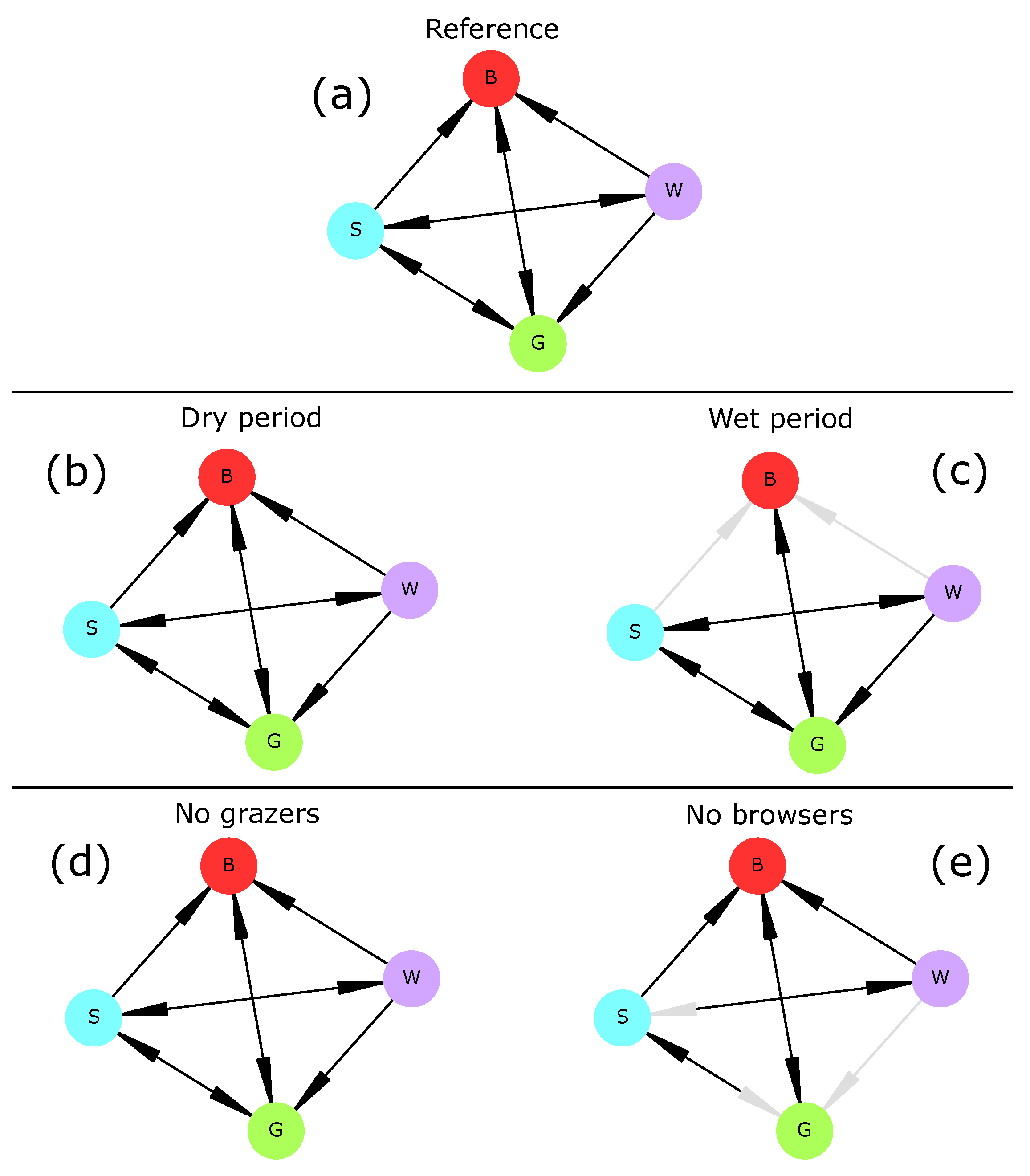
The reversibility of the STGs in all scenarios except the “dry period” suggests that the ecosystem is able to recover its initial state under most permanent changes. Only the “dry period” scenario displayed irreversible dynamics as the initial vegetation type (i.e., tree-grass coexistence) and socio-economic profile (a mix of agriculture, pastoralism, and tourism) could not be maintained. This invalidates hypothesis H1 which stated that any permanent change of the reference scenario would induce an irreversible ecosystem change.
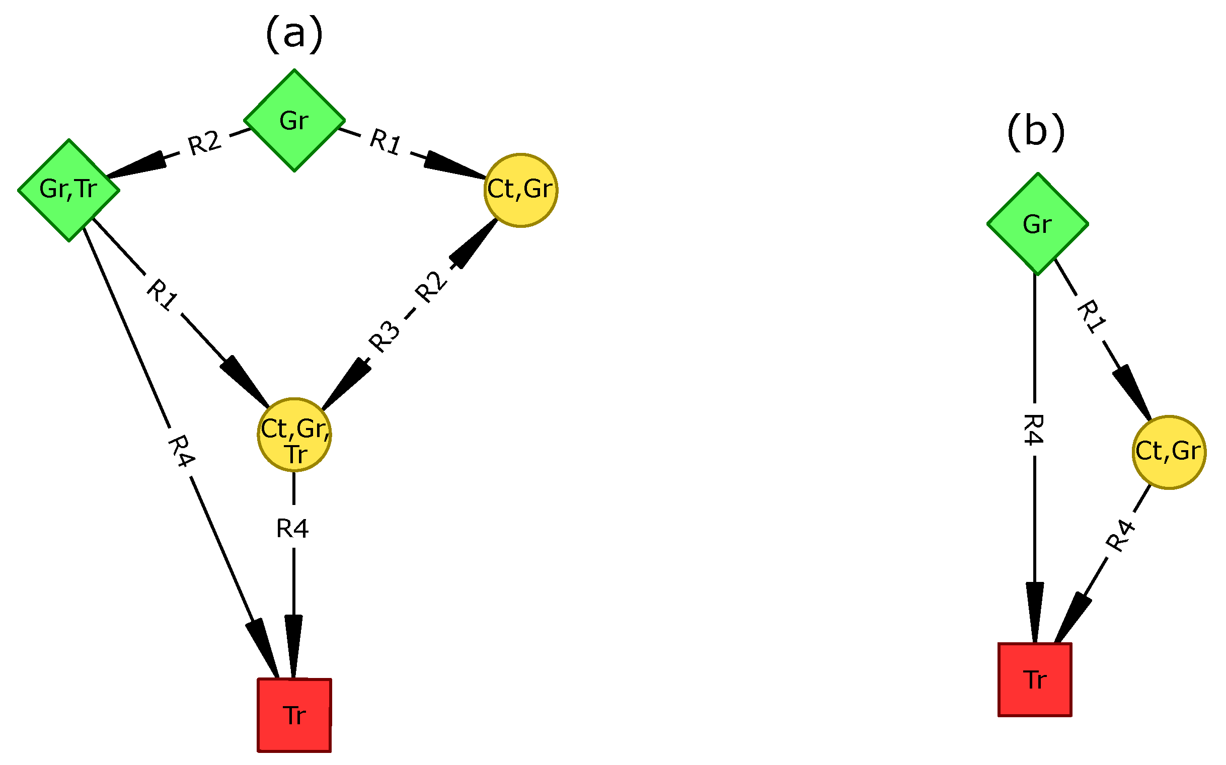
This result points to a need to clearly define reversibility and should be cautiously interpreted for at least two reasons. First, a reversible STG is defined by the existence of at least one path from any reachable state towards the initial state, which does not preclude the existence of potentially infinite trajectories (i.e., SCCs) inside it. For instance, in Figure 1a, the ecosystem may remain inside the SCC (an infinite trajectory) without never reaching the attractor. Therefore, STG reversibility should not be equated with resilience [79], but rather to a potential resilience. Second, our model is possibilistic and may thus include highly unlikely transitions. Therefore, using such models for management recommendations may require assessing the sensitivity of STG reversibility to rare events.

4.1. Vegetation Dynamics

Vegetation transitions are a major issue for rangeland ecology as current increase in woody cover (i.e., generally composed of unpalatable plant species) threatens socio-economic activities such as pastoralism and especially cattle production [
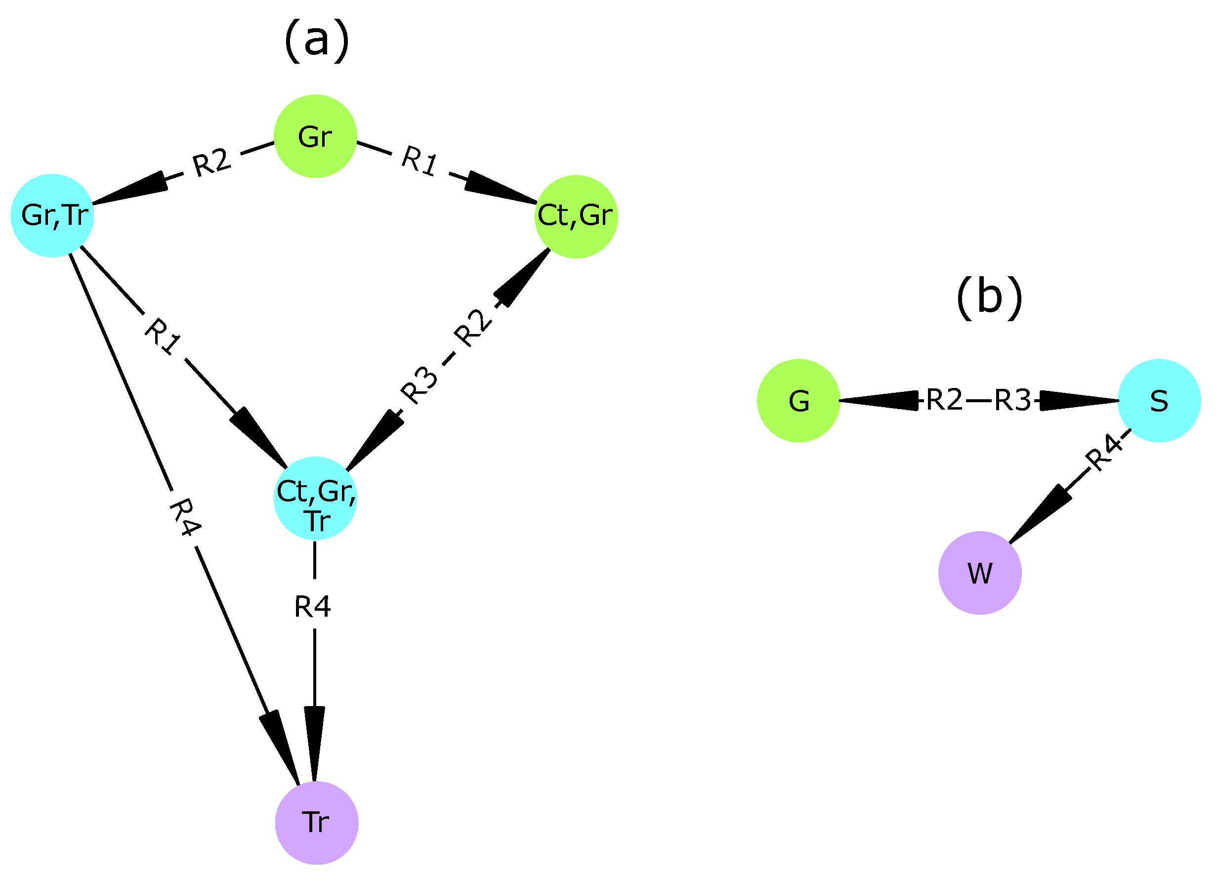
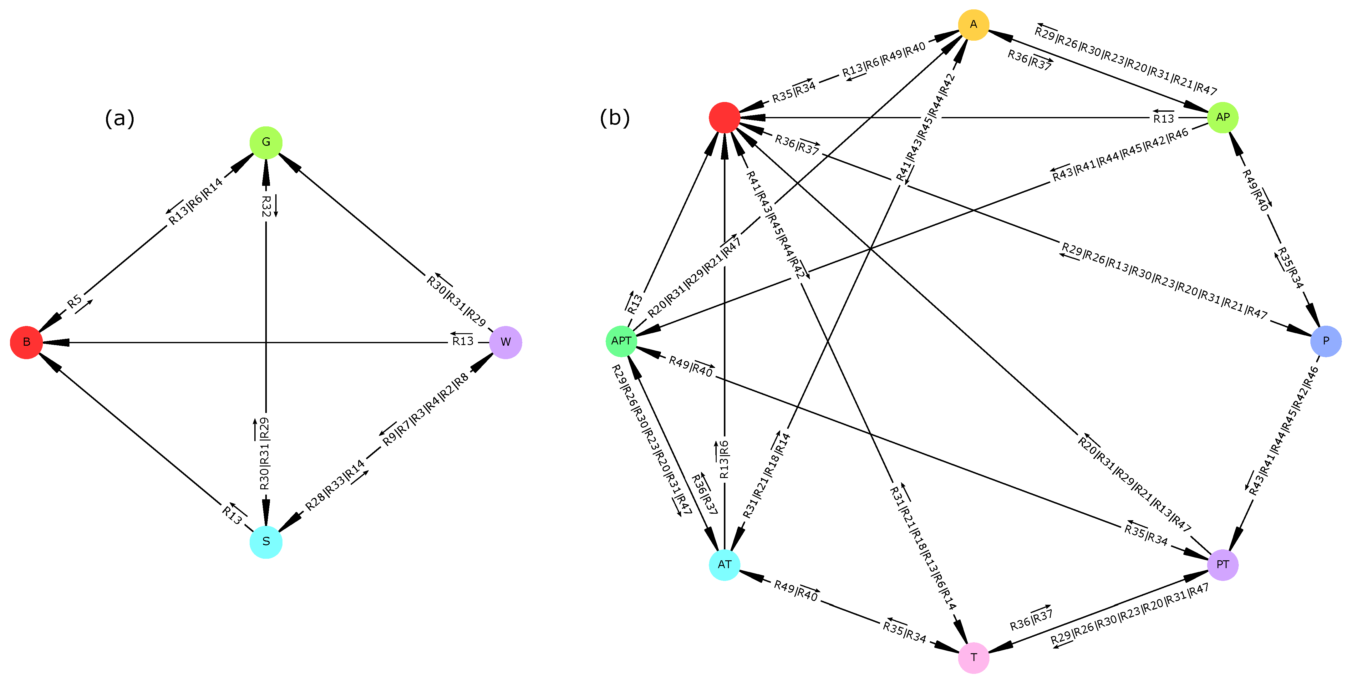
80]. Based on two plant types (grasses and trees), we defined four vegetation types, namely bare soil, grassland, savanna, and woodland.
In the reference scenario, all transitions establishing one plant type at a time were realized and all vegetation types were able to shift to bare soil. Predicted transitions were realistic as most have already been reported or hypothesized [60,81].
When subjected to a persistent lack of surface water (“dry period” scenario), the savanna vegetation (i.e., the initial vegetation type) underwent an irreversible shift towards a seasonal grassland in which woody plants could not establish (Figure A4). This transition was mediated by groundwater reserves, which requires the infiltration of surface water for being recharged (rule R11). The drying up of groundwater then affects woody plants which are assumed to rely on this resource (R32). Such drought-induced transitions have long been suggested [60,82]. Conversely, when water was non-limiting (“wet period” scenario), drought-induced transitions were not possible anymore, and thus transitions from savanna or woodland to bare soil were impossible. These two results do not invalidate hypothesis H2 and confirm the role of water availability in vegetation dynamics.
When herbivory was removed from the ecosystem (“no grazers” and “no browsers” scenarios), drought preserved most vegetation transitions. This was especially true for grazers whose extinction had no effect on vegetation transitions (Figure 2). This was not in agreement with current knowledge as grazing is known to favor trees over grasses [83]. Indeed, the only rule relating grazing mammals (here, livestock) and grasses was R14, i.e., overgrazing. This rule could be rewritten to better represent the effect of livestock (and grazing mammals in general) on the increase in woody cover. On the other hand, browsers were necessary to three transitions (Woodland→Grassland, Woodland→Savanna, and Savanna→Grassland) as those disappeared when browsers were removed from the system. Therefore, hypothesis H3 is invalidated and should be reassessed after model adjustments.
These results highlight the role of surface water (indirectly, through the watering of herbivores) and groundwater (directly, through its use by woody plants) as drivers of vegetation change [60,82,84,85,86]. Browsers contributed to a reduction in woody cover, which confirms current knowledge [87,88]. These general results support management recommendations about the preservation of wild herbivores for managing vegetation [81].
Fire and soil nutrients, which are not considered here, are well-known drivers of vegetation dynamics [82] and could easily be included in later model versions. The vegetation part of the model can be improved by adding more components to it (e.g., shrubs, bushes, or different life stages for trees) or accounting for other plant-water-herbivore interactions. Such an improvement could involve experts from this domain and/or new field surveys. Besides, vegetation summary graphs (Figure 2) share many similarities with State-and-Transition Models [21] which have been extensively used to represent rangeland or savanna dynamics [28,81].

4.2. Socio-Economic Dynamics

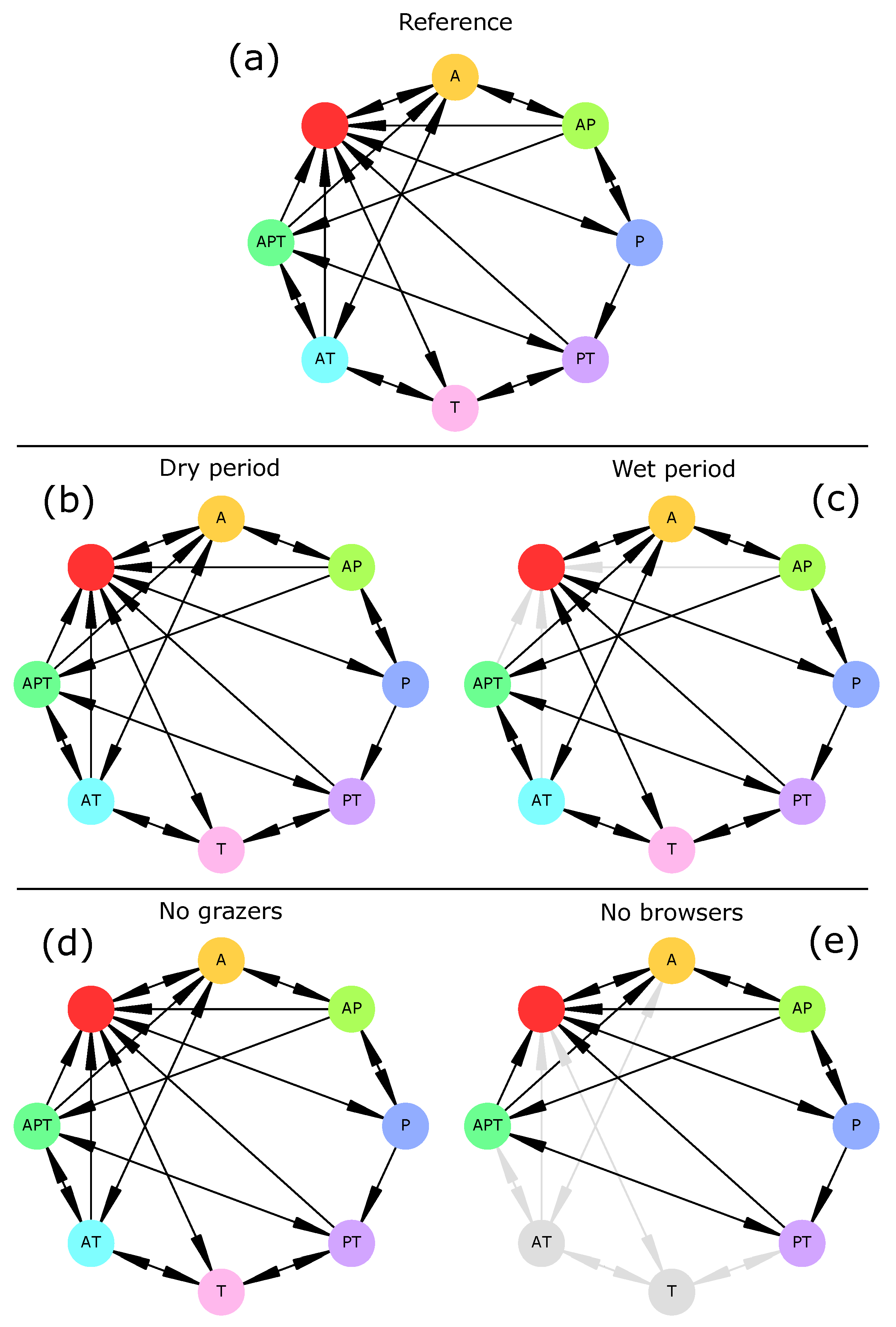
Socio-economic transitions describe the loss and development of new economic activities. Here, we focused on three activities, namely agriculture, pastoralism, and tourism, which substantially contribute to east-African economies. However, agriculture and pastoralism are affected by changes in rainfall frequency and intensity [89,90]. In our model, on one hand, water scarcity (“dry period scenario”) and subsequent lack of forage constrained livestock production and pushed the system into a regime of purely rainfed agriculture (Figure A4). For the same reasons, wildlife populations declined, thus making tourism disappear. This latter prediction corroborates other findings [91]. On the other hand, increasing water availability (“wet period” scenario) did not prevent any socio-economic profile (Figure 4). Rather, drought-induced transitions (here, general disruption of all socio-economic activities) disappeared. These results thus do not invalidate hypothesis H2.
The extinction of grazers and browsers had contrasting effects. The absence of grazers neither modified the set of reachable socio-economic profiles nor transitions compared to the reference scenario. On the contrary, the absence of browsers made tourism necessarily associated to pastoralism. We insist on the fact that this does not mean that they depended on each other. This is due to the fact that (1) cattle necessarily enter the system simultaneously to wild grazers when forage and water are available in the rainy season and (2) that cattle either leave the system simultaneously (through the lack of forage (C6), water scarcity (C9, C10), or diseases (R48)), or after (through cattle predation by carnivores (R19)) wild grazers. As in this scenario carnivores only rely on cattle and wild grazers (browsers are absent), once these preys have gone extinct, carnivores quickly go extinct, which deprives tourism of attraction. Herbivores diversity (species richness, abundance, and phylogenetic diversity) has been showed to be positively related to the number of tourists [92]. Although this relationship is likely to be driven by the interest for biodiversity per se, our results also suggest that herbivores diversity may play a role in maintaining tourism by sustaining predator populations. As for vegetation transitions, hypothesis H3 is partly invalidated as grazers did not affect socio-economic transitions, while browsers absence affected the dynamics.
Our results point to a link between herbivores diversity and socio-economic changes. Although this relationship may be explored in more detail (through another model), our model already suggest mechanisms relating these two aspects of the social-ecological system. This highlights the need, at least in some specific systems, to consider ecological and anthropogenic aspect integratively for designing management interventions.

4.3. From Predictions to Policy Implications

Although our model makes predictions, it is unable to provide management recommendations at this stage. What would be required for doing so? The first requirement is to find a clear agreement between predicted and observed dynamics for at least one specific location. Here, the agreement between predictions and data is partial (albeit groundwater availability and browsers indeed play a role in vegetation dynamics) and is not sufficient for providing recommendations. Second, even though predictions would be confirmed, management recommendations must benefit stakeholders (e.g., farmers, pastoralists, tourists, or wildlife managers) and thus, must be discussed before being proposed. This is not the case here as the aim of this study is mostly methodological and only involve stakeholders during model conception. Such discussions could however be pursued in the future. This is not an exhaustive list of the requirements for providing management recommendations from model predictions.
Nonetheless, this study provides some tools that may draw the attention of managers to EDEN models. For instance, the summary graphs presented share many similarities with State-and-Transition Models used for rangeland management and national parks [28,93]. The EDEN framework complements these empirical (i.e., non-formal) models by providing a mechanistic basis to ecosystem transitions and many tools to analyze them.

4.4. How to Cope with Model Structure Uncertainty

Generally, the presence or absence of specific variables and relations (i.e., model structure) is not certain and several model structures could correspond to available knowledge or observations. Such uncertainty could result from spatial heterogeneity [94] or temporal changes of interaction networks. Alternative model structures often lead to contrasting dynamics [95,96] and choosing the right one(s) is challenging. In this study, we considered a single model structure to which we applied four press perturbations manipulating the value of specific variables. However, rules are not equally well supported (Table A2). Instead of testing all possible alternative model structures (which would generate many ecologically meaningless models), we could use uncertain rules to generate alternative model structures. For instance, we assumed that cattle was able to exclude wild grazers (R22), while the reverse was assumed impossible. One way to assess the role of such uncertain rules (r) would be to exclude them in all possible combinations ( 2 r ) and verify a list of specific dynamical properties (e.g., vegetation transitions) for each of the 2 r corresponding STGs. The same method could be applied to rules definitions. For instance, rule R47 assumes that wild (Bw) and domestic (Go) browsers should co-occur to enable epidemics to emerge. However, in areas where browsers are now extinct, livestock are still subject to diseases [97]. Therefore, we could split this rule as R47a: Bw+, Rf+, Sw+ >> Bw-, Go-, and R47b: Go+, Rf+, Sw+ >> Bw-, Go-. These two rules can also be considered more parsimonious as goats and browsers can be subject to diseases independently of one another. Note that rules R47a and R47b are both general cases of R47 (their conditions include that of R47). Besides, automatically assessing dynamical properties of hundreds or thousands alternative models requires powerful and rigorous analysis tools. For that purpose, the visual analysis of summary graphs would be unworkable and should be replaced by model-checking techniques [50].

4.5. The Scope and Verification of EDEN Models

This study showed how the EDEN modeling framework can make use of qualitative information, which is often the most abundant (and sometimes the only) knowledge source. Despite its qualitative nature, it can be used to derive predictions and explanations about specific social-ecological issues.
Here, questions were related to (1) the reachability of specific states from the initial state (e.g., “is woodland reachable from initial state under dry conditions?”) and (2) the existence of some transitions under various environmental conditions (e.g., “is the woodland-grassland transition possible under wet conditions?”). Such questions, or propositions, can be verified or refuted (e.g., “this state is not reachable” or “this transitions is impossible”). In addition, results can be “causally” explained, as studying model rules enables to identify which rule sequences (ecological events) are disrupted or forced by changes in environmental conditions. This form of event-based explanations may thus be promising for providing a coarse-grained mechanistic understanding of ecosystem trajectories. However, this by-hand explanation (by the visual examination of rules) is prone to errors and may require automated tools to be made more rigorous. Beside the comparison of model trajectories with observations, validation/refutation can be extended to the driving events behind them (approximated by model rules), i.e., assessing whether predicted trajectories are consistent with observed states and events. Model verification can also be improved by the use of model-checking techniques [52] which enable the automatic exploration of large ecological State-Transition Graphs [50]. Experts and managers may play a key role in this validation/refutation process and help designing and improving models, especially through State-and-Transition Models [21]. In return, researchers can provide modeling tools to derive predictions from this abundant expert knowledge. Ultimately, this interaction between ecosystem management and modeling may be used to improve management interventions.

5. Conclusions

In this study, we proposed the EDEN modeling framework as a tool for computing trajectories of an ecosystem from a qualitative knowledge base in the form of “if-then” rules. This qualitative and possibilistic model aims to predict and explain ecosystem trajectories by the interplay between multiple socio-economic and ecological events.
Here, we chose to apply this framework for modeling the socio-economic and ecological aspects of an east African savanna. We focused on vegetation and socio-economic transitions and showed that a reduction in surface water may lead to a disruption of socio-economic activities and biodiversity which is mediated by groundwater reserves and herbivores. Removing grazers or browsers herbivores had contrasting effects and highlighted the potential role of drought in controlling woody cover by itself.
The EDEN framework is qualitative, which means that it cannot provide precise (i.e., quantitative) predictions. In addition, the model is non-deterministic and non-probabilistic, which implies that its predictions cannot be assigned a probability. However, these two “limitations” have an interesting counterpart: The model does not require quantitative data about parameters describing observed phenomena, and its predictions are robust to changes in parameters or to uncertain measurements. Therefore, they are more general, more parsimonious, albeit less precise and certain. Although rules may be more descriptive than explanatory (e.g., rules driving seasonality), they correspond to observed phenomena, can be easily explained and thus enable the use of expert-knowledge.
This study is a first step and the EDEN framework is still evolving. It has the potential to bridge, on one hand, expert knowledge, e.g., derived from rangeland managers who design State-and-Transition Models, and, on the other hand, modeling through an intuitive event-based approach. Such models could find applications in agroecology to assess the long-term impacts of management actions on biodiversity and livelihoods.

Author Contributions

Conceptualization, M.C.; Data curation, C.H., P.P., C.T., A.T. and C.G.; Formal analysis, M.C.; Funding acquisition, C.T. and C.G.; Investigation, M.C., P.P. and C.G.; Methodology, M.C., C.H., F.P. and C.G.; Resources, F.P.; Software, F.P.; Supervision, C.H. and C.G.; Validation, M.C.; Writing—original draft, M.C.; Writing—review & editing, M.C., C.H., P.P. and A.T. All authors have read and agreed to the published version of the manuscript.

Funding

This research was funded by the HATARI (HAzard in TAnzanian RIft) Project under the CNRS Tellus-Rift program.

Acknowledgments

We warmly thank Colin Thomas for his technical support with analyses. We also thank the three anonymous reviewers for their valuable comments on our manuscript.

Conflicts of Interest

The authors declare no conflict of interest.

Abbreviations

    The following abbreviations are used in this manuscript:
EDENEcological Discrete-Event Network
STGState-Transition Graph
SCCStrongly Connected Component
HTGHierarchical Transition Graph

Appendix A. Study Area Description

Gelai plains are located in the East African Rift, south of Lake Natron, and are part of the Tarangire-Manyara ecosystem [98] and the Maasailand. These grass-dominated plains have volcanic ash-derived alkaline soils. Indeed, their proximity with the Ol Doinyo Lengai stratovolcano, with its natrocarbonatite lava and ashes, strongly influences soil pH. Woody vegetation is confined to adjacent reliefs [99] and vegetation changes are mainly driven by water availability and herbivory [58,100]. Mean annual precipitation strongly varies seasonally and inter-annually [62]. This high variability constrains primary, but also secondary production since the Gelai plains are important calving grounds for wildebeest populations [98]. The Gelai plains also provide resources for Maasai pastoralists and their cattle, goat, and sheep herds. Agriculture is practiced but confined to village surroundings and wetter areas [62]. Lake Natron, Mount Kitumbeine, and Ol Doinyo Lengai are also important touristic sites, adding another economic value to this ecosystem. On the other hand, northern-Meru savannas are more densely populated. The different ethnics have contrasting economic activities, characterized by the respective roles of agriculture and pastoralism during the year [63]. Villages and local authorities manage socio-economic activities by allowing water resources use, preventing overgrazing, and regulating tourism. Their decisions also affect pathogen exchanges, vaccination, pest management, and/or spatial and temporal grazing regulations. NGOs, such as Oikos, play a major role in improving livelihoods, promoting local development, and sustainable practices. The area exchanges many goods and services with the Arusha city, which is located south to the mount Meru.

Appendix B. Model Variables

Appendix B.1. How We Chose Variables

The choice of variables was constrained by (spatial and temporal) scales and research questions. Rainfall was chosen to represent the seasons (Rf+: rainy season; Rf-: dry season), while surface water (Sw) and groundwater (Gw) were defined according to their role for plants and animals, which are crucial for addressing our research questions. Indeed, surface water is used by wildlife and livestock for watering, while groundwater is assumed to be mostly used by trees and not by grasses, following the “two-layer hypothesis” [101,102,103]. Soil moisture was included in earlier versions but was removed since it is highly correlated to rainfall events. We chose to keep the wildlife component simple in this first model, by considering the dominant functional groups known to affect either herbivore populations (Ca: carnivores), trees (Bw: browsers; El: elephants), or grasses (Gz: grazers). These four groups are present and abundant in east Africa, and are known to exert a pressure on plant dynamics, which justifies their presence in the model (they would have been absent if we aimed to model a present-day west African savanna, where many of these mammals have gone extinct). The pastoral component (Ct: cattle; Go: goats) is restricted to livestock. Pastoralists were mentioned in earlier versions, but their close dependence on livestock (and reciprocally, livestock depends on pastoralists) made their explicit representation useless for our research questions. The same reasoning applies for farmers with crops. In addition, the fact that these two human groups are implicit enables to account for agropastoral households (families both practicing farming and livestock husbandry). On the other hand, tourists are not related to a specific production (livestock or crops) and were thus represented by themselves. The vegetation component was represented by grasses (Gr) and trees (Tr) to keep the model simple. We initially included tree saplings in order to represent intermediate tree life stages but finally kept them implicit as vegetation transitions were well represented by these two variables.

Appendix B.2. How to Make This Choice More Replicable?

The first way to improve the choice of variables is to make it standardized and replicable. This includes (non-exhaustively) automated (i.e., replicable) literature reviews and standardized field surveys (with rigorous protocols for observations and interviews). Once collected in the literature and in the field, information must be selected according to research objectives. This includes identifying events in the literature, i.e., changes in the qualitative state of a variable, which amounts to its discretization (in our case, in two values + and −). Standardized discretization methods have been discussed in systems biology. From this standardized collection and discretization of data, rules can be built.

Appendix C. Model Rules

Rules represent events, i.e., changes in system state. When an event occurs from a state, it produces a transition which generates a new state. In the EDEN framework, transition durations are not considered. Some events are considered too fast to be explicitly considered and are thus represented as constraints. For instance, if a pond dries up, we expect fishes living in it to die (almost) simultaneously. Therefore, we neglect the time interval between the event “the pond dries up” and the event “fishes die” by qualifying the latter event as a constraint. Constraints have priority over rules and thus, no rule can be executed as long as a constraint is satisfied. Hence, the state “the pond is dry and fishes are alive” satisfies a constraint and prevents other rules executions. Thereafter, we remove all states satisfying a constraint because they are considered too fast (or too transient) and irrelevant for our questions.
Table A1. Model constraints. Ecologically similar constraints share the same interpretation. Note the slight differences (in condition) between the various groups of plants and animals with respect to their resource requirements (food or water). Model scenarios correspond to versions of the reference scenarios in which some constraints have been added to represent a “press perturbation”, i.e., maintaining the value of some variables constant. Within a scenario (e.g., “No grazers”) all corresponding constraints are activated (i.e., C11 and C12).
ConditionRealizationInterpretationReferences
C1Ct-, Bw-, Ca-, El-, Go-, Gz-To-Without any attraction, tourism disappears.CS
C2Gr-, Tr-El-Without food resources, wildlife and livestock die or migrate.CS
C3Gr-Ct-, Gz-CS
C4Tr-Bw-, Go-CS
C5Ct-, Bw-, Go-, Gz-Ca-CS
C6Gw-, Rf-, Sw-Ct-, Bw-, Ca-, El-, Go-, Gz-Without water resources, wildlife, livestock and plants (including crops) die or migrate.CS
C7Rf-, Sw-Ct-, Ca-, Gz-CS
C8Gw-, Rf-Cr-, Gr-, Tr-A
C9Sw+Sw-“Dry period” scenario
C10Sw-Sw+“Wet period” scenario
C11Ct+Ct-“No grazers” scenario
C12Gz+Gz-
C13Bw+Bw-“No browsers” scenario
C14Go+Go-
C15El+El-
Therefore, qualifying an event as a “regular” rule or a constraint is partly arbitrary and depends on the scientific question. For the aforementioned reasons, states satisfying a constraint are considered transient, and may be removed prior to analysis (as we did here). Note, however, that transient states may be considered in order to keep all states while recognizing that some events must have priority over others.
Table A2. Model rules. Rules with similar descriptions are grouped within the same multirow. A: Assumption, FO: Field observation or report from experts.
ConditionRealizationInterpretationReferences
R1Bw-, El-, Go-, Rf-, Tr+Rf+, Sw+Rainy season switch. If (1) at least one browsers group exert a pressure on woody plants or (2) trees are rare, then grass can grow. [76]
R2Bw+, Rf-, Tr+Gr+, Rf+, Sw+ [76]
R3El+, Rf-, Tr+Gr+, Rf+, Sw+ [76]
R4Go+, Rf-, Tr+Gr+, Rf+, Sw+ [76]
R5Rf-, Tr-Gr+, Rf+, Sw+ [76], FO
R6Rf+Rf-Dry seasonA
R7Bw+, Rf+, Tr+Gr+Grass growthFO
R8El+, Rf+, Tr+Gr+FO
R9Go+, Rf+, Tr+Gr+FO
R10Rf+, Tr-Gr+
R11Rf+, Sw+Gw+In rainy season, aquifers may fill up, while in dry season, surface and groundwater may sequentially dry up. [104]
R12Rf-Sw- [104]
R13Rf-, Sw-Gw- [104]
R14Ct+, Rf-Gr-In dry season, non-managed livestock may overgraze the area. [105]
R15Gz+Ca+Wild herbivores (preys) may increase carnivore populations.A
R16Bw+Ca+A
R17Ca+Gz-Carnivores may strongly affect wild herbivores populations.A
R18Ca+Bw-A
R19Bw-, Ca+, Gz-Ct-Without managers support to protect livestock, carnivores may attack livestock if wildlife populations are low. [106]
R20Bw-, Ca+, Gz-Go- [106]
R21Rf-, Sw-Bw-, El-, Go-Low water availability may lead browser and generalist herbivores to leave the area. [107,108]
R22Ct+Gz-Herbivores may outcompte one another.A
R23El+, Gr-Go-A
R24Go+, Gr-El-A
R25Go+Bw-A
R26Bw+Go-A
R27El+Bw-A
R28Gr+, Gw+, Rf+, Tr+Gr-Trees outcompete grasses at high water availability. [75]
R29Go+Gr+, Tr-All browsers may strongly affect woody plants cover and favor grasses. [109]
R30El+Gr+, Tr- [64,109,110]
R31Bw+Gr+, Tr- [109,111,112]
R32Bw-, El-, Go-, Gr+, Gw+, Rf+Tr+In rainy season, the absence of browsers may promote tree recruitment. [75]
R33Gr+, Gw+, Rf-, Tr+Gr-In dry season, trees maintain a higher productivity than grasses due to their deeper root system. [76]
R34Rf+Cr+In rainy season, rainfall and surface water enable rain-fed farming as well as animals watering. In dry season, groundwater pumping enable irrigated agriculture and watering livestock. [113,114]
R35Gw+, Rf-Cr+ [115]
R36Gw+, Sw-, Tr+Go+ [116]
R37Sw+, Tr+Bw+, El+, Go+FO
R38Gw+, Sw-, Gr+Ct+ [116]
R39Sw+, Gr+Ct+, El+, Gz+FO
R40El+Cr-Elephants may destroy crop fields.FO and [5]
R41Gz+To+Wildlife and traditional pastoral culture may attract tourists.FO
R42El+To+FO
R43Bw+To+FO
R44Ca+To+FO
R45Ct+To+FO
R46Go+To+FO
R47Bw+, Go+, Rf+, Sw+Bw-, Go-Browsers may die from diseases. [117]
R48Ct+, Gz+, Rf+, Sw+Ct-, Gz-Grazers may die from diseases. [117]
R49Rf+Cr-In rainy season, pest may destroy crops. [118]

Appendix D. Model Scenarios

As mentioned in Table A1, scenarios result from the application of constraints. These constraints are disabled in the reference scenario and each specific set of constraint is enabled for each scenario.
These constraints make some states impossible, and thus prevent some rules executions. This explains the observed differences between STGs and vegetation or socio-economic transitions.
Table A3. General properties each scenario’s STG. STG size: Number of states; reversibility: Each reachable state from the initial state can reach back the initial state; attractors: “Itself” if the whole STG is reversible or indicates the number of attractors (i.e., either stable states or inescapable SCCs).
ScenarioSTG SizeReversibleAttractors
Reference482Yesitself
Dry period163No1
Wet period390Yesitself
No grazers302Yesitself
No browsers106Yesitself

Appendix D.1. Reference

The STG of reference scenario has 482 states (Figure A1) and is reversible (i.e., forms a unique SCC). Its complexity prevents any analysis by hand, thus justifying the use of summary graphs to simplify its dynamics (Figure 2 and Figure 4).
Figure A1. STG of the reference scenario. Graph nodes and edges represent ecosystem states and transitions, respectively. This STG consists of 482 states and 2640 transitions. Nodes color is arbitrary.
Land 11 00042 g0a1
Figure A2. Vegetation and socio-economic summary graphs of the reference scenario. Summary graphs (a,b) are the same as Figure 2 and Figure 4, respectively, and indicate the rules involved in each transition. In (a) node labels indicate vegetation types as defined in Section 2.6, with B: Bare soil; G: Grassland; S: Savanna, and W: Woodland, while in (b) they indicate socio-economic profiles, i.e., combinations of socio-economic activities A, P, and T, with A: Agriculture; P: Pastoralism, and T: Tourism. Small arrows associated to each transition labels (rules) indicate to which transition are associated the considered group of rules (see Table A2 for details about rules).
Land 11 00042 g0a2

Appendix D.2. “Dry Period” Scenario

Appendix D.2.1. The Hierarchical Transition Graph

The “dry period” scenario is the only scenario exhibiting an irreversible STG. Trajectories converge towards a small (three states) SCC attractor. One convenient way to represent such a graph is to draw its Hierarchical Transition Graph (HTG, for formal definitions, see, [73]). A HTG merges as single nodes SCCs (depicted as round nodes), basins of attraction (i.e., sets of states necessarily ending up in a stable state, generally depicted as squares) and basins (i.e., states not belonging to a SCC nor a basin of attraction and leading to the same SCCs or stable states, depicted as lozenges). It is an acyclic graph focusing only irreversible aspects of system dynamics (Figure A3).
Figure A3. Comparison between the STG and HTG of the “Grasses-Trees-Cattle” toy model. (a) This STG is the same as Figure 1a and rules are those from Table 1. In (b), green lozenges nodes belong to a basin, yellow round nodes belong to a SCC and the red square node to a stable state (i.e., a basin of attraction of one state). (b) The HTG resulting from the merging of corresponding nodes in (a) into a single node. Hence the green lozenge and yellow round nodes include two states each and their “internal” transitions (e.g., the R2-R3 oscillation) are “hidden” within them. Node labels correspond to active variables Gr: Grasses, Tr: Trees, and Ct: Cattle. Note that in (b) node labels correspond to variables that are present in all states of the topological structure (i.e., SCC, basin or stable state). For instance, Tr oscillates in the yellow SCC in (a) and is thus not mentioned in the corresponding yellow node in (b).
Land 11 00042 g0a3

Appendix D.2.2. The Attractor

The “dry period” attractor is not a stable state and is not cyclic. Some authors have proposed to call it a complex attractor (i.e., involving intertwined cycles [119]). Indeed, while the whole attractor is a cycle, it also comprises two small cycles (R5–R6 and R34–R49) (see Table A2 for rules details). Ecologically, this attractor represents an ecosystem regime in which periodic rainfall drives a seasonal grassland and enables a rain-fed agriculture. This is further confirmed by the fact that when the rainy season stops (R6), grass and crops disappear until the next rains (R5). One fundamental issue here is the existence of an infinite rainy season driven by the loop R35–R50. Resolving this issue is beyond the scope of this paper, but one possible solution is to force, during model analysis, to only consider trajectories in which the rainy season is necessarily followed by a dry season, and reciprocally (i.e., to apply a fairness constraint on seasonality).
Figure A4. STG of the attractor of the “dry period” scenario. Graph nodes and edges represent ecosystem states and transitions, respectively. Node labels correspond to active variables, with Rf: Rainfall, Gr: Grass, and Cr: Crops. Edge labels correspond to rules driving transitions (see Table A2). Node color is arbitrary.
Land 11 00042 g0a4

References

  1. Marchant, R. Understanding complexity in savannas: Climate, biodiversity and people. Curr. Opin. Environ. Sustain. 2010, 2, 101–108. [Google Scholar] [CrossRef]
  2. Ryan, C.M.; Pritchard, R.; McNicol, I.; Owen, M.; Fisher, J.A.; Lehmann, C. Ecosystem services from southern African woodlands and their future under global change. Philos. Trans. R. Soc. B Biol. Sci. 2016, 371. [Google Scholar] [CrossRef]
  3. Huntly, N. How Important Are Consumer Species to Ecosystem Functioning? In Linking Species & Ecosystems; Jones, C.G., Lawton, J.H., Eds.; Springer: Boston, MA, USA, 1995; pp. 72–83. [Google Scholar] [CrossRef]
  4. McNaughton, S.J.; Ruess, R.W.; Seagle, S.W. Large Mammals and Process Dynamics in African Ecosystems. BioScience 1988, 38, 794–800. [Google Scholar] [CrossRef]
  5. Sinclair, A.R.E. (Ed.) Serengeti III: Human Impacts on Ecosystem Dynamics; University of Chicago Press: Chicago, IL, USA, 2008; OCLC: ocn183928576. [Google Scholar]
  6. Ellis, J.E.; Swift, D.M. Stability of African pastoral ecosystems: Alternate paradigms and implications for development. J. Range Manag. 1988, 41, 450–459. [Google Scholar] [CrossRef] [Green Version]
  7. Wolanski, E.; Gereta, E. Water quantity and quality as the factors driving the Serengeti ecosystem, Tanzania. Hydrobiologia 2001, 458, 169–180. [Google Scholar] [CrossRef]
  8. Larsen, F.; Hopcraft, J.G.C.; Hanley, N.; Hongoa, J.R.; Hynes, S.; Loibooki, M.; Mafuru, G.; Needham, K.; Shirima, F.; Morrison, T.A. Wildebeest migration drives tourism demand in the Serengeti. Biol. Conserv. 2020, 248, 108688. [Google Scholar] [CrossRef]
  9. Little, P.D. Pastoralism, biodiversity, and the shaping of savanna landscapes in East Africa. Africa 1996, 66, 37–51. [Google Scholar] [CrossRef]
  10. Pratt, D.J.; Gwynne, M.D.; Blackie, J.R. Rangeland Management and Ecology in East Africa; Hodder and Stoughton: London, UK, 1977. [Google Scholar]
  11. Hély, C.; Bremond, L.; Alleaume, S.; Smith, B.; Sykes, M.T.; Guiot, J. Sensitivity of African biomes to changes in the precipitation regime. Glob. Ecol. Biogeogr. 2006, 15, 258–270. [Google Scholar] [CrossRef]
  12. Hein, L. The impacts of grazing and rainfall variability on the dynamics of a Sahelian rangeland. J. Arid Environ. 2006, 64, 488–504. [Google Scholar] [CrossRef]
  13. Sinclair, A.R.E.; Metzge, K.L.; Mduma, S.A.R.; Fryxell, J.M. (Eds.) Serengeti IV: Sustaining Biodiversity in a Coupled Human-Natural System; The University of Chicago Press: Chicago, IL, USA, 2015. [Google Scholar]
  14. Touboul, J.D.; Staver, A.C.; Levin, S.A. On the complex dynamics of savanna landscapes. Proc. Natl. Acad. Sci. USA 2018, 115, E1336–E1345. [Google Scholar] [CrossRef] [Green Version]
  15. Kauffman, S. Metabolic stability and epigenesis in randomly constructed genetic nets. J. Theor. Biol. 1969, 22, 437–467. [Google Scholar] [CrossRef]
  16. Levins, R. The strategy of model building on population biology. Am. Sci. 1966, 54, 421–431. [Google Scholar]
  17. Thomas, R. Regulatory networks seen as asynchronous automata: A logical description. J. Theor. Biol. 1991, 153, 1–23. [Google Scholar] [CrossRef]
  18. Bashari, H.; Smith, C.; Bosch, O.J.H. Developing decision support tools for rangeland management by combining state and transition models and Bayesian belief networks. Agric. Syst. 2008, 99, 23–34. [Google Scholar] [CrossRef]
  19. Archer, S. Have Southern Texas Savannas Been Converted to Woodlands in Recent History? Am. Nat. 1989, 134, 545–561. [Google Scholar] [CrossRef]
  20. Bélisle, A.C.; Asselin, H.; LeBlanc, P.; Gauthier, S. Local knowledge in ecological modeling. Ecol. Soc. 2018, 23. [Google Scholar] [CrossRef]
  21. Westoby, M.; Walker, B.; Noy-Meir, I. Opportunistic Management for Rangelands Not at Equilibrium. J. Range Manag. 1989, 42, 266. [Google Scholar] [CrossRef]
  22. Levins, R. Qualitative Analysis of Partially Specified Systems. Ann. N. Y. Acad. Sci. 1974, 231, 123–138. [Google Scholar] [CrossRef] [PubMed]
  23. Bredeweg, B.; Salles, P.; Neumann, M. Ecological Applications of Qualitative Reasoning. In Ecological Informatics: Scope, Techniques and Applications; Recknagel, F., Ed.; Springer: Berlin/Heidelberg, Germany, 2006; pp. 15–47. [Google Scholar] [CrossRef]
  24. Robeva, R.; Murrugarra, D. The spruce budworm and forest: A qualitative comparison of ODE and Boolean models. Lett. Biomath. 2016, 3, 75–92. [Google Scholar] [CrossRef]
  25. Gaucherel, C.; Théro, H.; Puiseux, A.; Bonhomme, V. Understand ecosystem regime shifts by modeling ecosystem development using Boolean networks. Ecol. Complex. 2017, 31, 104–114. [Google Scholar] [CrossRef]
  26. Zhao, Y.; Largouët, C.; Cordier, M.O. EcoMata, un logiciel d’aide à la décision pour améliorer la gestion des écosystèmes. Ingénierie Des Systèmes D’information 2011, 16, 85–111. [Google Scholar] [CrossRef] [Green Version]
  27. Dambacher, J.M.; Li, H.W.; Rossignol, P.A. Qualitative predictions in model ecosystems. Ecol. Model. 2003, 161, 79–93. [Google Scholar] [CrossRef]
  28. Bestelmeyer, B.T.; Ash, A.; Brown, J.R.; Densambuu, B.; Fernández-Giménez, M.; Johanson, J.; Levi, M.; Lopez, D.; Peinetti, R.; Rumpff, L.; et al. State and Transition Models: Theory, Applications, and Challenges. In Rangeland Systems: Processes, Management and Challenges; Briske, D.D., Ed.; Springer Series on Environmental Management; Springer International Publishing: Cham, Switzerland, 2017; pp. 303–345. [Google Scholar] [CrossRef] [Green Version]
  29. Salles, P.; Bredeweg, B. Modelling population and community dynamics with qualitative reasoning. Ecol. Model. 2006, 195, 114–128. [Google Scholar] [CrossRef]
  30. Starfield, A.M. Qualitative, Rule-Based Modeling. BioScience 1990, 40, 601–604. [Google Scholar] [CrossRef]
  31. Rykiel, E.J. Artificial intelligence and expert systems in ecology and natural resource management. Ecol. Model. 1989, 46, 3–8. [Google Scholar] [CrossRef]
  32. Justus, J. Loop analysis and qualitative modeling: Limitations and merits. Biol. Philos. 2007, 21, 647–666. [Google Scholar] [CrossRef]
  33. Matthewson, J.; Weisberg, M. The structure of tradeoffs in model building. Synthese 2009, 170, 169–190. [Google Scholar] [CrossRef] [Green Version]
  34. Paulevé, L.; Kolčák, J.; Chatain, T.; Haar, S. Reconciling qualitative, abstract, and scalable modeling of biological networks. Nat. Commun. 2020, 11, 4256. [Google Scholar] [CrossRef]
  35. Hosack, G.R.; Hayes, K.R.; Dambacher, J.M. Assessing Model Structure Uncertainty Through an Analysis of System Feedback and Bayesian Networks. Ecol. Appl. 2008, 18, 1070–1082. [Google Scholar] [CrossRef]
  36. Puccia, C.J.; Levins, R. Qualitative Modeling in Ecology: Loop Analysis, Signed Digraphs, and Time Averaging. In Qualitative Simulation Modeling and Analysis; Luker, P.A., Schmidt, B., Fishwick, P.A., Luker, P.A., Eds.; Springer: New York, NY, USA, 1991; Volume 5, pp. 119–143. [Google Scholar] [CrossRef]
  37. Saadatpour, A.; Albert, R. A comparative study of qualitative and quantitative dynamic models of biological regulatory networks. EPJ Nonlinear Biomed. Phys. 2016, 4. [Google Scholar] [CrossRef] [Green Version]
  38. Drake, J.A.; Zimmerman, C.R.; Purucker, T.; Rojo, C. On the nature of the assembly trajectory. In Ecological Assembly Rules: Perspectives, Advances, Retreats; Weiher, E., Keddy, P., Eds.; Cambridge University Press: Cambridge, UK, 1999; pp. 233–250. [Google Scholar] [CrossRef]
  39. Cosme, M.; Thomas, C.; Gaucherel, C. On the History of Ecosystem Dynamic Modeling: The Rise and Promises of Qualitative Models. BioSystems 2022. Submitted. [Google Scholar]
  40. Cassandras, C.G.; Lafortune, S. Introduction to Discrete EVENT Systems, 2nd ed.; Springer: New York, NY, USA, 2008. [Google Scholar]
  41. Cordier, M.O.; Largouet, C.; Zhao, Y. Model-Checking an Ecosystem Model for Decision-Aid. In Proceedings of the 2014 IEEE 26th International Conference on Tools with Artificial Intelligence, Limassol, Cyprus, 10–12 November 2014; pp. 539–543. [Google Scholar] [CrossRef] [Green Version]
  42. Abou-Jaoudé, W.; Monteiro, P.T.; Naldi, A.; Grandclaudon, M.; Soumelis, V.; Chaouiya, C.; Thieffry, D. Model Checking to Assess T-Helper Cell Plasticity. Front. Bioeng. Biotechnol. 2015, 2. [Google Scholar] [CrossRef] [Green Version]
  43. Béal, J.; Pantolini, L.; Noël, V.; Barillot, E.; Calzone, L. Personalized logical models to investigate cancer response to BRAF treatments in melanomas and colorectal cancers. PLoS Comput. Biol. 2021, 17, e1007900. [Google Scholar] [CrossRef]
  44. Campbell, C.; Yang, S.; Albert, R.; Shea, K. A network model for plant–pollinator community assembly. Proc. Natl. Acad. Sci. USA 2011, 108, 197–202. [Google Scholar] [CrossRef] [PubMed] [Green Version]
  45. Campbell, C.; Yang, S.; Shea, K.; Albert, R. Topology of plant-pollinator networks that are vulnerable to collapse from species extinction. Phys. Rev. E 2012, 86, 021924. [Google Scholar] [CrossRef] [PubMed] [Green Version]
  46. Campbell, C.; Yang, S.; Albert, R.; Shea, K. Plant–pollinator community network response to species invasion depends on both invader and community characteristics. Oikos 2015, 124, 406–413. [Google Scholar] [CrossRef]
  47. Gronewold, A.; Sonnenschein, M. Event-based modeling of ecological systems with asynchronous cellular automata. Ecol. Model. 1998, 108, 37–52. [Google Scholar] [CrossRef]
  48. Gaucherel, C.; Carpentier, C.; Geijzendorffer, I.R.; Noûs, C.; Pommereau, F. Discrete-event models for conservation assessment of integrated ecosystems. Ecol. Inform. 2020, 101205. [Google Scholar] [CrossRef]
  49. Mao, Z.; Centanni, J.; Pommereau, F.; Stokes, A.; Gaucherel, C. Maintaining biodiversity promotes the multifunctionality of social-ecological systems: Holistic modeling of a mountain system. Ecosyst. Serv. 2021, 47. [Google Scholar] [CrossRef]
  50. Thomas, C.; Cosme, M.; Gaucherel, C.; Pommereau, F. Model-checking ecological state-transition graphs. bioRxiv 2021. [Google Scholar] [CrossRef]
  51. Bestelmeyer, B.T.; Tugel, A.J.; Peacock, G.L.; Robinett, D.G.; Shaver, P.L.; Brown, J.R.; Herrick, J.E.; Sanchez, H.; Havstad, K.M. State-and-Transition Models for Heterogeneous Landscapes: A Strategy for Development and Application. Rangel. Ecol. Manag. 2009, 62, 1–15. [Google Scholar] [CrossRef] [Green Version]
  52. Clarke, E.M.; Henzinger, T.A.; Veith, H.; Bloem, R. (Eds.) Handbook of Model Checking; Springer International Publishing: Cham, Switzerland, 2018. [Google Scholar] [CrossRef]
  53. Gaucherel, C.; Pommereau, F. Using discrete systems to exhaustively characterize the dynamics of an integrated ecosystem. Methods Ecol. Evol. 2019, 10, 1615–1627. [Google Scholar] [CrossRef] [Green Version]
  54. Plant, R.E.; Vayssieres, M.P.; Greco, S.E.; George, M.R.; Adams, T.E. A Qualitative Spatial Model of Hardwood Rangeland State-and-Transition Dynamics. J. Range Manag. 1999, 52, 51. [Google Scholar] [CrossRef]
  55. Gillson, L. A large infrequent disturbance’ in an East African savanna. Afr. J. Ecol. 2006, 44, 458–467. [Google Scholar] [CrossRef]
  56. Bobe, R. The evolution of arid ecosystems in eastern Africa. J. Arid Environ. 2006, 66, 564–584. [Google Scholar] [CrossRef]
  57. Ogutu, J.O.; Piepho, H.P.; Dublin, H.T.; Bhola, N.; Reid, R.S. El Niño-Southern Oscillation, rainfall, temperature and Normalized Difference Vegetation Index fluctuations in the Mara-Serengeti ecosystem. Afr. J. Ecol. 2008, 46, 132–143. [Google Scholar] [CrossRef]
  58. Sankaran, M.; Ratnam, J.; Hanan, N. Woody cover in African savannas: The role of resources, fire and herbivory. Glob. Ecol. Biogeogr. 2008, 17, 236–245. [Google Scholar] [CrossRef]
  59. Li, Q.; Staver, A.C.; E, W.; Levin, S.A. Spatial feedbacks and the dynamics of savanna and forest. Theor. Ecol. 2019, 12, 237–262. [Google Scholar] [CrossRef]
  60. Breshears, D.D.; Knapp, A.K.; Law, D.J.; Smith, M.D.; Twidwell, D.; Wonkka, C.L. Rangeland Responses to Predicted Increases in Drought Extremity. Rangelands 2016, 38, 191–196. [Google Scholar] [CrossRef] [Green Version]
  61. Chamaillé-Jammes, S.; Fritz, H.; Murindagomo, F. Climate-driven fluctuations in surface-water availability and the buffering role of artificial pumping in an African savanna: Potential implication for herbivore dynamics. Austral Ecol. 2007, 32, 740–748. [Google Scholar] [CrossRef]
  62. Gereta, E.; Ole Meing’ataki, G.E.; Mduma, S.; Wolanski, E. The role of wetlands in wildlife migration in the Tarangire ecosystem, Tanzania. Wetl. Ecol. Manag. 2004, 12, 285–299. [Google Scholar] [CrossRef]
  63. Istituto Oikos. The Mount Meru Challenge: Integrating Conservation and Development in Northern Tanzania; Technical Report; Ancoma Libri: Milano, Italy, 2011. [Google Scholar]
  64. Laws, R.M. Elephants as Agents of Habitat and Landscape Change in East Africa. Oikos 1970, 21, 1. [Google Scholar] [CrossRef]
  65. Mitchell, J.; Slim, H. Listening to Rural People in Africa: The Semi-structured Interview in Rapid Rural Appraisal. Disasters 1991, 15, 68–72. [Google Scholar] [CrossRef]
  66. D’Amario, S.C.; Rearick, D.C.; Fasching, C.; Kembel, S.W.; Porter-Goff, E.; Spooner, D.E.; Williams, C.J.; Wilson, H.F.; Xenopoulos, M.A. The prevalence of nonlinearity and detection of ecological breakpoints across a land use gradient in streams. Sci. Rep. 2019, 9, 3878. [Google Scholar] [CrossRef] [Green Version]
  67. Hillel, D. Soil moisture and seed germination. In Plant Responses and Control of Water Balance; Kozlowski, T.T., Ed.; Academic Press: Cambridge, MA, USA, 1972; pp. 65–89. [Google Scholar] [CrossRef]
  68. Garg, A.; Di Cara, A.; Xenarios, I.; Mendoza, L.; De Micheli, G. Synchronous versus asynchronous modeling of gene regulatory networks. Bioinformatics 2008, 24, 1917–1925. [Google Scholar] [CrossRef] [PubMed] [Green Version]
  69. Clarke, L. Possibilistic Thinking: A New Conceptual Tool for Thinking about Extreme Events. Soc. Res. 2008, 75, 669–690. [Google Scholar]
  70. Kristensen, N.P.; Chisholm, R.A.; McDonald-Madden, E. Dealing with high uncertainty in qualitative network models using Boolean analysis. Methods Ecol. Evol. 2019, 10, 1048–1061. [Google Scholar] [CrossRef]
  71. de Wit, M.; Stankiewicz, J. Changes in Surface Water Supply Across Africa with Predicted Climate Change. Science 2006, 311, 1917–1921. [Google Scholar] [CrossRef] [Green Version]
  72. Staver, A.C.; Abraham, J.O.; Hempson, G.P.; Karp, A.T.; Faith, J.T. The past, present, and future of herbivore impacts on savanna vegetation. J. Ecol. 2021, 109, 2804–2822. [Google Scholar] [CrossRef]
  73. Bérenguier, D.; Chaouiya, C.; Monteiro, P.T.; Naldi, A.; Remy, E.; Thieffry, D.; Tichit, L. Dynamical modeling and analysis of large cellular regulatory networks. Chaos Interdiscip. J. Nonlinear Sci. 2013, 23, 025114. [Google Scholar] [CrossRef]
  74. Diop, O.; Tourniel, L.; Fromion, V. Summarizing complex asynchronous Boolean attractors, application to the analysis of a mammalian cell cycle model. In Proceedings of the 2019 18th European Control Conference (ECC), Naples, Italy, 25–28 June 2019; pp. 1677–1682. [Google Scholar] [CrossRef]
  75. Devine, A.P.; McDonald, R.A.; Quaife, T.; Maclean, I.M.D. Determinants of woody encroachment and cover in African savannas. Oecologia 2017, 183, 939–951. [Google Scholar] [CrossRef] [Green Version]
  76. February, E.C.; Higgins, S.I.; Bond, W.J.; Swemmer, L. Influence of competition and rainfall manipulation on the growth responses of savanna trees and grasses. Ecology 2013, 94, 1155–1164. [Google Scholar] [CrossRef]
  77. Homewood, K.; Rodgers, W.A. Maasailand Ecology: Pastoralist Development and Wildlife Conservation in Ngorongoro, Tanzania, 1st ed.; Cambridge University Press: Cambridge, UK, 2004. [Google Scholar]
  78. Scholes, R.J.; Archer, S.R. Tree-Grass Interactions in Savannas. Annu. Rev. Ecol. Syst. 1997, 28, 517–544. [Google Scholar] [CrossRef]
  79. Holling, C.S. Resilience and Stability of Ecological Systems. Annu. Rev. Ecol. Syst. 1973, 4, 1–23. [Google Scholar] [CrossRef] [Green Version]
  80. Angassa, A. The effect of clearing bushes and shrubs on range condition in Borana, Ethiopia. Trop. Grasslands 2002, 36, 69–76. [Google Scholar]
  81. Liao, C.; Clark, P.E. Rangeland vegetation diversity and transition pathways under indigenous pastoralist management regimes in southern Ethiopia. Agric. Ecosyst. Environ. 2018, 252, 105–113. [Google Scholar] [CrossRef]
  82. Skarpe, C. Dynamics of savanna ecosystems. J. Veg. Sci. 1992, 3, 293–300. [Google Scholar] [CrossRef]
  83. Holdo, R.M.; Holt, R.D.; Fryxell, J.M. Grazers, browsers, and fire influence the extent and spatial pattern of tree cover in the Serengeti. Ecol. Appl. 2009, 19, 95–109. [Google Scholar] [CrossRef]
  84. Case, M.F.; Wigley-Coetsee, C.; Nzima, N.; Scogings, P.F.; Staver, A.C. Severe drought limits trees in a semi-arid savanna. Ecology 2019, 100, e02842. [Google Scholar] [CrossRef]
  85. Fensham, R.J.; Laffineur, B.; Allen, C.D. To what extent is drought-induced tree mortality a natural phenomenon? Glob. Ecol. Biogeogr. 2019, 28, 365–373. [Google Scholar] [CrossRef]
  86. Koppel, J.V.D.; Prins, H.H.T. The importance of herbivore interactions for the dynamics of African savanna woodlands: An hypothesis. J. Trop. Ecol. 1998, 14, 565–576. [Google Scholar] [CrossRef] [Green Version]
  87. Voysey, M.D.; Archibald, S.; Bond, W.J.; Donaldson, J.E.; Carla Staver, A.; Greve, M. The role of browsers in maintaining the openness of savanna grazing lawns. J. Ecol. 2021, 109, 913–926. [Google Scholar] [CrossRef]
  88. Staver, A.C.; Bond, W.J.; Stock, W.D.; van Rensburg, S.J.; Waldram, M.S. Browsing and fire interact to suppress tree density in an African savanna. Ecol. Appl. 2009, 19, 1909–1919. [Google Scholar] [CrossRef]
  89. Kirkbride, M.; Grahn, R. Survival of the Fittest: Pastoralism and Climate Change in East Africa; Technical Report 116; Oxfam International: Nairobi, Kenya, 2008. [Google Scholar]
  90. Yanda, P.Z.; Mung’ong’o, C.G.; cha Dar es Salaam, C.K. (Eds.) Pastoralism and Climate Change in East Africa; Mkuki na Nyota Publishers Ltd: Dar es Salaam, Tanzania, 2016. [Google Scholar]
  91. Kilungu, H.; Leemans, R.; Munishi, P.K.T.; Amelung, B. Climate Change Threatens Major Tourist Attractions and Tourism in Serengeti National Park, Tanzania. In Climate Change Adaptation in Africa: Fostering Resilience and Capacity to Adapt; Leal Filho, W., Belay, S., Kalangu, J., Menas, W., Munishi, P., Musiyiwa, K., Eds.; Climate Change Management; Springer International Publishing: Cham, Switzerland, 2017; pp. 375–392. [Google Scholar] [CrossRef]
  92. Arbieu, U.; Grünewald, C.; Martín-López, B.; Schleuning, M.; Böhning-Gaese, K. Large mammal diversity matters for wildlife tourism in Southern African Protected Areas: Insights for management. Ecosyst. Serv. 2018, 31, 481–490. [Google Scholar] [CrossRef]
  93. Provencher, L.; Frid, L.; Czembor, C.; Morisette, J.T. State-and-Transition Models: Conceptual Versus Simulation Perspectives, Usefulness and Breadth of Use, and Land Management Applications. In Exotic Brome-Grasses in Arid and Semiarid Ecosystems of the Western US: Causes, Consequences, and Management Implications; Germino, M.J., Chambers, J.C., Brown, C.S., Eds.; Springer Series on Environmental Management; Springer International Publishing: Cham, Switzerland, 2016; pp. 371–407. [Google Scholar] [CrossRef]
  94. Marzloff, M.P.; Dambacher, J.M.; Johnson, C.R.; Little, L.R.; Frusher, S.D. Exploring alternative states in ecological systems with a qualitative analysis of community feedback. Ecol. Model. 2011, 222, 2651–2662. [Google Scholar] [CrossRef]
  95. Schwab, J.D. Concepts in Boolean network modeling: What do they all mean? Comput. Struct. Biotechnol. J. 2020, 18, 571–582. [Google Scholar] [CrossRef]
  96. Hulot, F.D.; Lacroix, G.; Lescher-Moutoué, F.; Loreau, M. Functional diversity governs ecosystem response to nutrient enrichment. Nature 2000, 405, 340–344. [Google Scholar] [CrossRef]
  97. Richard, D.; Alary, V.; Corniaux, C.; Duteurtre, G.; Lhoste, P. Dynamique des Élevages Pastoraux et Agropastoraux en Afrique Intertropicale; Éditions Quae: Versailles, France, 2019. [Google Scholar] [CrossRef]
  98. Morrison, T.A.; Bolger, D.T. Connectivity and bottlenecks in a migratory wildebeest Connochaetes taurinus population. Oryx 2014, 48, 613–621. [Google Scholar] [CrossRef] [Green Version]
  99. Reed, D.N.; Anderson, T.M.; Dempewolf, J.; Metzger, K.; Serneels, S. The spatial distribution of vegetation types in the Serengeti ecosystem: The influence of rainfall and topographic relief on vegetation patch characteristics. J. Biogeogr. 2009, 36, 770–782. [Google Scholar] [CrossRef]
  100. Asner, G.P.; Levick, S.R.; Kennedy-Bowdoin, T.; Knapp, D.E.; Emerson, R.; Jacobson, J.; Colgan, M.S.; Martin, R.E. Large-scale impacts of herbivores on the structural diversity of African savannas. Proc. Natl. Acad. Sci. USA 2009, 106, 4947–4952. [Google Scholar] [CrossRef] [PubMed] [Green Version]
  101. Walter, H. Grasland, Savanne und Busch der arideren Teile Afrikas in ihrer ökologischen Bedingtheit. In Jahrbücher für Wissenschaftliche Botanik; 1939; pp. 750–860. Available online: https://books.google.com.hk/books/about/Grasland.html?id=ZkhkxAEACAAJ&redir_esc=y (accessed on 26 November 2021).
  102. Ward, D.; Wiegand, K.; Getzin, S. Walter’s two-layer hypothesis revisited: Back to the roots! Oecologia 2013, 172, 617–630. [Google Scholar] [CrossRef] [Green Version]
  103. Holdo, R.M. Revisiting the Two-Layer Hypothesis: Coexistence of Alternative Functional Rooting Strategies in Savannas. PLoS ONE 2013, 8, e69625. [Google Scholar] [CrossRef] [PubMed]
  104. Arnold, J.G.; Allen, P.M.; Bernhardt, G. A comprehensive surface-groundwater flow model. J. Hydrol. 1993, 142, 47–69. [Google Scholar] [CrossRef]
  105. Schlesinger, W.H.; Reynolds, J.F.; Cunningham, G.L.; Huenneke, L.F.; Jarrell, W.M.; Virginia, R.A.; Whitford, W.G. Biological Feedbacks in Global Desertification. Science 1990, 247, 1043–1048. [Google Scholar] [CrossRef] [Green Version]
  106. Mponzi, B.; Lepczyk, C.; Kissui, M. Characteristics and Distribution of Livestock Losses Caused by Wild Carnivores in Maasai Steppe of Northern Tanzania. Human—Wildlife Interact. 2014, 8, 10. [Google Scholar] [CrossRef]
  107. Western, D. Water availability and its influence on the structure and dynamics of a savannah large mammal community. Afr. J. Ecol. 1975, 13, 265–286. [Google Scholar] [CrossRef]
  108. Smit, I.P.; Grant, C.C.; Devereux, B.J. Do artificial waterholes influence the way herbivores use the landscape? Herbivore distribution patterns around rivers and artificial surface water sources in a large African savanna park. Biol. Conserv. 2007, 136, 85–99. [Google Scholar] [CrossRef]
  109. O’Kane, C.A.; Duffy, K.J.; Page, B.R.; Macdonald, D.W. Are the long-term effects of mesobrowsers on woodland dynamics substitutive or additive to those of elephants? Acta Oecologica 2011, 37, 393–398. [Google Scholar] [CrossRef]
  110. Staver, A.C.; Bond, W.J. Is there a ‘browse trap’? Dynamics of herbivore impacts on trees and grasses in an African savanna. J. Ecol. 2014, 102, 595–602. [Google Scholar] [CrossRef]
  111. Augustine, D.J.; Mcnaughton, S.J. Regulation of shrub dynamics by native browsing ungulates on East African rangeland: Browsing ungulates and shrubland dynamics. J. Appl. Ecol. 2004, 41, 45–58. [Google Scholar] [CrossRef]
  112. Levick, S.; Rogers, K. Patch and species specific responses of savanna woody vegetation to browser exclusion. Biol. Conserv. 2008, 141, 489–498. [Google Scholar] [CrossRef]
  113. Smaling, E.; Dixon, J. Adding a soil fertility dimension to the global farming systems approach, with cases from Africa. Agric. Ecosyst. Environ. 2006, 116, 15–26. [Google Scholar] [CrossRef]
  114. Maeda, E.E.; Clark, B.J.; Pellikka, P.; Siljander, M. Modelling agricultural expansion in Kenya’s Eastern Arc Mountains biodiversity hotspot. Agric. Syst. 2010, 103, 609–620. [Google Scholar] [CrossRef]
  115. Kashimbiri, N.; Mtalo, F.; Mwanuzi, F.; Mandal, N.C.; Singh, V.S. Modelling the Impact of Urbanization on Groundwater Using System Dynamic Technique. A Case Study of Arusha Municipal Well Field in Northeastern Tanzania. Tanzan. J. Eng. Technol. 2009, 32, 67–80. [Google Scholar] [CrossRef]
  116. Chamaillé-Jammes, S.; Charbonnel, A.; Dray, S.; Madzikanda, H.; Fritz, H. Spatial Distribution of a Large Herbivore Community at Waterholes: An Assessment of Its Stability over Years in Hwange National Park, Zimbabwe. PLoS ONE 2016, 11, e153639. [Google Scholar] [CrossRef] [Green Version]
  117. Hampson, K.; Lembo, T.; Bessell, P.; Auty, H.; Packer, C.; Halliday, J.; Beesley, C.A.; Fyumagwa, R.; Hoare, R.; Ernest, E.; et al. Predictability of anthrax infection in the Serengeti, Tanzania: Predicting anthrax infection in the Serengeti. J. Appl. Ecol. 2011, 48, 1333–1344. [Google Scholar] [CrossRef] [PubMed] [Green Version]
  118. Gregory, P.J.; Johnson, S.N.; Newton, A.C.; Ingram, J.S.I. Integrating pests and pathogens into the climate change/food security debate. J. Exp. Bot. 2009, 60, 2827–2838. [Google Scholar] [CrossRef] [PubMed]
  119. Naldi, A.; Remy, E.; Thieffry, D.; Chaouiya, C. Dynamically consistent reduction of logical regulatory graphs. Theor. Comput. Sci. 2011, 412, 2207–2218. [Google Scholar] [CrossRef]
Figure 1. Transition graphs of the “Grasses-Trees-Livestock” toy model (Table 1). (a) State-Transition Graph (STG) depicting every reachable states and transitions from the initial state, with node labels corresponding to active variables Gr (Grasses), Tr (Trees), and Ct (Cattle). (b) Vegetation summary graph depicting transitions between vegetation types. This graph was made from (a) by merging nodes of the same color. In both graphs, node colors correspond to vegetation types, with green for grassland (G; defined as Gr+, Tr-), blue for savanna (S; Gr+, Tr+), and purple for woodland (W; Gr-, Tr+). Note that some rules may be defined and never be executed (e.g., R5).
Land 11 00042 g001
Figure 2. Vegetation transitions for each scenario. Vegetation summary graphs for (a) the reference scenario, (b) the “dry period”, (c) the “wet period”, (d) “no grazers”, and (e) “no browsers”. Node labels indicate vegetation types as defined in Section 2.6, with B: Bare soil; G: Grassland; S: Savanna, and W: Woodland. Node colors are arbitrary and correspond to vegetation types. Grayed out edges are absent from the graph and highlight differences relative to reference scenario. Grayed out arrow tips (e) indicate when a bidirectional transition becomes unidirectional.
Land 11 00042 g002
Figure 3. Hierarchical Transition Graph (HTG) of the “dry period” scenario. The same HTG is represented with a focus on either vegetation (a) and socio-economic (b) dynamics. Graph nodes are SCCs and each transition is, by definition, irreversible. Therefore, dynamics within each node display some form of oscillation. Letters correspond to vegetation types (B: Bare soil; G: Grassland; S: Savanna; W: Woodland) or socio-economic activities (A: Agriculture; P: Pastoralism; T: Tourism). In (a), node labels either correspond to a stable vegetation type (e.g., “S”) or to an oscillation between two (e.g., “G-B”) or more (“various”) types. In (b), node labels correspond to socio-economic activities. An activity can be stable, and is thus noted by a letter (for instance, T in “A*T”). When the activity can change (oscillate) in a SCC, it is noted with a * (as in, A*T, where A is oscillating).
Land 11 00042 g003
Figure 4. Socio-economic transitions for each scenario. Socio-economic summary graphs for (a) the reference scenario, (b) the “dry period”, (c) the “wet period”, (d) “no grazers”, and (e) “no browsers”. Node labels indicate socio-economic profiles, i.e., combinations of socio-economic activities A, P, and T, with A: Agriculture; P: Pastoralism, and T: Tourism. Non-gray node colors are arbitrary and correspond to socio-economic profiles. Grayed out nodes and edges are absent from the graph and highlight differences relative to the reference scenario.
Land 11 00042 g004
Table 1. Rule set of the “Grasses-Trees-Cattle” toy model. Variables are Gr (Grasses), Tr (Trees), and Ct (Cattle), which mostly consumes grasses.
Condition RealizationInterpretation
R1Gr+Ct+Grasses attract cattle.
R2Gr+Tr+Grasses promote tree growth.
R3Ct+, Gr+Tr-Cattle control trees if there is enough grass.
R4Tr+Gr-, Ct-Trees outcompete grasses and thus exclude cattle.
R5Tr-Gr+Grasses reestablish if trees are cut.
Table 2. Variables and their initial value.
AcronymVariableDescriptionInitial Value
RfRainfallSeasonal rainfall+
SwSurface waterAny reservoir where mammals water+
GwGroundwaterWater below the grass root zone+
CaCarnivoresGrazers’ or browsers’ predators+
GzGrazersMammals feeding on grasses+
ElElephantsElephant population+
BwBrowsersMammals feeding on woody plants+
CtCattleCattle breeds+
GoGoatsGoat breeds+
GrGrassesMostly Poaceae+
TrTreesWoody plants+
CrCropsRainfed and irrigated crops+
ToTouristsPeople attracted by wildlife and pastoral livelihoods+
Table 3. Vegetation and socio-economic partitions. Each partition consists of several groups that are defined by state properties (i.e., the values of specific variables). Symbols ∧ and ∨ correspond to the logical AND and OR, respectively. Agriculture (A) = Cr+, Pastoralism (P) = (Ct+ Go+), and Tourism (T) = To+. Groups within a partition are mutually exclusive.
PartitionsGroupsState Properties
Vegetation typesBare soil (B) T r G r
Grassland (G) T r G r +
Savanna (S) T r + G r +
Woodland (W) T r + G r
Socio-economic profilesAPT C r + ( C t + G o + ) T o +
AP C r + ( C t + G o + ) T o
AT C r + ( C t G o ) T o +
AP C r + ( C t + G o + ) T o
PT C r ( C t + G o + ) T o +
A C r + ( C t G o ) T o
P C r ( C t + G o + ) T o
T C r ( C t G o ) T o +
C r ( C t G o ) T o
Publisher’s Note: MDPI stays neutral with regard to jurisdictional claims in published maps and institutional affiliations.

