A GIS-Based Simulation Method for Regional Food Potential and Demand

Abstract

A quantitative assessment of food-water-energy interactions is important to assess pathways and scenarios towards a holistically sustainable regional development. While a range of tools and methods exist that assess energetic demands and potentials on a regional scale, the same is not true for assessments of regional food demand and potential. This work introduces a new food simulation workflow to address local food potential and demand at the regional level, by extending an existing regional energy-water simulation platform. The goal of this work is to develop a GIS-based bottom-up approach to simulate regional food demand that can be linked to similarly GIS-based workflows assessing regional water demands and energetic demands and potentials. This allows us to study food-water-energy issues on a local scale. For this, a CityGML land use data model is extended with a feed and animal potential raster map as well as a soil type map to serve as the main inputs. The workflow simulates: (1) the vegetal and animal product food potentials by taking climate, crop type, soil type, organic farming, and food waste parameters into account; (2) the food demand of vegetal and animal products influenced by population change, body weight, age, human development index, and other indicators. The method is tested and validated in three German counties with various land use coverages. The results show that restricting land used exclusively for energy crop production is the most effective way to increase annual food production potential. Climate change by 2050 is expected to result in annual biomass yield changes between −4% and 2% depending on the region. The amount of animal product consumption is expected to rise by 16% by 2050, while 4% fewer vegetal products are excepted to be consumed.

1. Introduction

Human demands for the consumption of food, water, and energy are forecast to continue to rise in the coming decades [1]. The challenge will be to meet these increasing demands sustainably across all dimensions [2]. Given the fact that natural resources do not operate in isolation, a detailed recognition of their influences on one another is required [3]. Therefore, a food potential simulation serves as an important element within the framework of the food-water-energy (FWE) nexus and allows us to, for example, study the impact of regional food production potentials on local bioenergy or free-field PV potential and vice versa.

Generally, a food system includes the elements of food production, harvesting, storage, processing, transportation, and consumption [4]. Due to their complexity, the understanding of food system dynamics and the consequences of their rapid transformations is still limited [5]. Indicators such as food security, biodiversity, food safety, or nutrition factors that quantify the performance of energy system are chosen by countries and organizations [5]. In this paper, the consumers’ food demand, which includes the minimal nutritious demand, storage, and waste for end consumers, and food production potential, which represents the calorie amount of food potential stored in biomass, are emphasized and addressed.

On the demand side, the change of diet and its impact on cropland use were studied in [6] and typical diets pattern and their projection are shown in [7]. Both studies showed that the long-term nutrition state was improving, and food consumption patterns moved from low to higher calorie diets. With socio-economic development, population growth rates decreased and diets changed: typically, consumption of animal protein, vegetable oils, fruits, and vegetables increased, while starchy staples became less important [6]. In food balance analysis, average statistical per-capita food availability values at a national level were usually used [8]. To identify the influencing factors to food intake demand, the method introduced in [9] provided the average per-capita food energy intake at the national level depending on the age, sex, country, birth rate, and population.

On the supply side, assessing yearly biomass mass potentials locally is the first step towards a regional food potential analysis. For such an analysis at the sub-country or country level, the most common way of acquiring crop production data is through statistical portals [8,10,11,12]. The advantage of this approach was its accuracy; however, statistical values are usually aggregated to the country or sub-country level and follow the administration boundary. Highly aggregated yield values, thus, lead to uncertainties if regional and sub-regional crop yield assessments are required, i.e., the statistical aggregated yield varies locally due to distinctly local climate and soil situations. To downscale the national yield data to a higher spatial resolution, a gridded crop yield raster map with a resolution of 5′ was adopted in [13]. Still, the data was static from statistical sources without the possibility to study the influences of, e.g., climate change and irrigation. Moreover, food waste is not considered in this study. Rosenberg et al. simulated the potential changes for crops, only including wheat, rice, maize, and soybeans, caused by climate change at the global level using compatible crop models. The impacting factors included the current mix of rainfed and irrigated production, today’s crop varieties, nitrogen management, and agricultural soils. However, the method was site-specific and aggregated to the national level [14].

Several studies analyzed the food inequality between food supply and consumption across countries and sub-regions adapting GIS (Geographic Information System) methods [10,15]. Merem et al. analyzed food security by presenting and comparing collected data with GIS methods at the national level. Without simulating socio-economic and natural environmental influences, the paper only presented grain food potential without distinguishing vegetable and animal food potential at the national aggregated level [15]. Khushi et al. investigated how disaggregated data on food consumption, nutrient demand, and production of major commodities on a sub-national level could be interlinked in the GIS environment to spatially analyze food consumption inequalities [10]. The food production was taken from statistical sources aggregated to the county (district) level. This restricts the approach to (i) a higher resolution, e.g., urban surroundings, and (ii) certain external environment changes, e.g., climate change. Furthermore, Beltran–Pena et al. performed an integrated, global assessment that considers a range of factors affecting future food production and demand until 2100 at the national level [11]. Driven by its scale, highly aggregated values at the national level and assumptions were used, e.g., the per-capita calorie demand is constant for all scenarios and regions, and climate change effects are considered only for certain crop types.

A regional food potential simulation tool is thus missing, which: (i) simulates the food potential using a bottom-up approach based on a dynamic biomass yield simulator for all crop types, considering impact factors including local climate, crop type distribution, or soil texture distribution; (ii) can be applied to any chosen region without strictly following administrative boundaries at any level of scale, i.e., from community to county to federal state; (iii) builds on commonly available GIS data models for both potential and demand analysis; (iv) is integrated into an energy-water simulation platform [16], that can simulate the roof PV potential [17], heat demand [17], electricity profile [18], water demand [19], and bioenergy [20] to complete the workflow sets for assessing FWE nexus effects. This allows studies of trade-offs between local energy and food potentially on the same land areas by also considering constraints of local water resources—even more so after the workflows that assess free land PV and wind onshore potentials are finished.

The objective of this paper was to investigate regional food consumption and production potential with a high geographical resolution, building on commonly available digital landscape models as a key input on the supply side, as well as on the demand side if population data is missing. The goal was not to rival more specialized tools that focus on food demand or supply, but to extend an existing water-energy simulation platform with a reasonably accurate workflow for assessing regional food supply-demand balances and to thus be able to investigate trade-offs along the food-water-energy nexus at any regional scale. To give an example, a combination of the workflows allows us to assess the energetic benefits of applying wind onshore or free-field PV to varying degrees on different forms of land, and their impacts on irrigation water demand and local food production potential.

Regional food potential was simulated by extending an existing GIS-based biomass workflow based on food-related GIS data, e.g., crop calorie value, food waste, and animal product amounts (Section 2.1). Regional food demands are simulated by multiplying occupant numbers based on CityGML (City Geography Markup Language) 3D building objects and per-capita calorie demand considering several socio-economic indicators (Section 2.2). Three representative case study counties in Germany were chosen (Section 2.3) and used for validation (Section 2.4) and sensitivity analysis (Section 2.5).

2. Materials and Methods

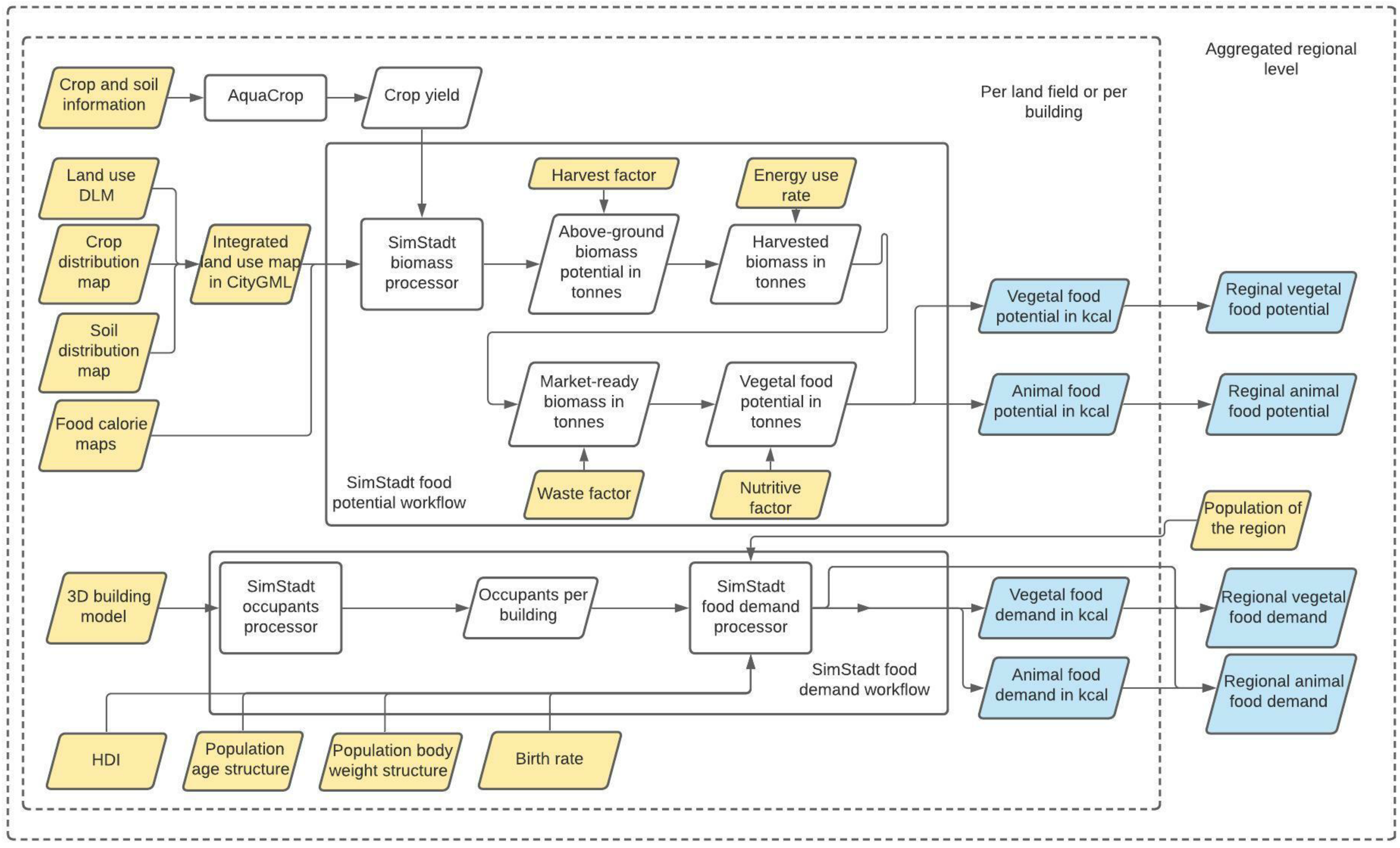
Figure 1 gives an overview of the input (yellow) and output (blue) data and methods used in this study. SimStadt, which has been under constant development at HFT Stuttgart since 2012 [16], comprises a modular workflow management, with each workflow serving a specific purpose. To date, it can assess building-related demands (cooling and heating [21,22], residential electricity [18], water [19]) and renewable energy potential (rooftop photovoltaics [17] and biomass [20,23]) on a single-building or single-field level using 3D city models or digital landscape models in the CityGML format. CityGML is an open standardized data model and exchange format to store digital 3D models of cities and landscapes [24]. The biomass workflow which integrates the dynamic yield simulation tool AquaCrop [25] applies a bottom-up approach to simulate the biomass yield in weight as well as the technical bioenergy potential for each land polygon covered with biomass. This biomass workflow is used as a basis for the newly-established food potential workflow.

Table 1. List of data used for this study.

Data	Spatial Resolution	Unit	Source
Nutritive factor	Per crop type	Kcal/100 g	Food and Agriculture Organization (FAO) [29]
Food waste rate	Per crop type	%	FAO [30]
DLM land use map	1:10,000/1:25,000 of the topographic objects; ±3 m for linear objects	ha−1	AdV [26]
Crop type distribution	30 m	ha−1	Griffiths, Nendel et al. (2019) [27]
Soil distribution	1:100,000 (1 km)	ha−1	BGR [31]
Precipitation	Region	mm/a	Meteonorm [32]
Temperature	Region	°C	Meteonorm [32]
Atmospheric CO2 concentration	Region	ppm	FAO
Dietary pattern projection	Country	Kcal/cap/day	Kastner et al.; Pradhan et al. [6,7]
The factor of animal products out of local crop potential	5 arc min (around 6 km in southern Germany)	%	Pradhan et al. [13]

shows the (spatial) resolution and the sources of the input data. The topographic inputs include land use, crop distribution, a soil distribution map, and a food calorie map. The land use map consists of Digital Landscape Model (DLM) data from Germany’s Official Real Property Cadaster Information System (ALKIS) [26]. The DLM map consists of several object types, including building, waterbody, vegetation, or transportation. Since the land area dedicated to transportation purposes is stored as a line plus a buffer width, it can overlap with the vegetation layer, and the shared part of the vegetation layer needs to be cut out to avoid its inflation. DLM data accurately indicated the boundary and main usage of each land polygon. However, the specific crop type growing on polygons classified as agricultural land was missing. To fill this gap, the DLM data was combined with satellite data on crop types distribution from [27]. Plant-soil relationships in the surface soil layer affect crop productivity [28]. For this, a soil map for Germany from the Federal Institute for Geosciences and Natural Resources (BGR) was adopted. This map shows the distribution of typical soil types in the topsoils.

On top of these maps, climate data (precipitation, atmospheric temperature, and irradiance) for current and predicted situations were taken from Meteonorm [32]. The climatic data is available in hourly resolution for a chosen year. AquaCrop simulates the yields of all possible crops on all possible soil for biomass processors to use.

With the above-mentioned integrated land use maps, including information on land use, crop distribution, soil distribution, and climatic data, the biomass potential in weight was calculated with a single land polygon resolution. On top of this, food calorie maps from Pradhan et al. provide information and a global gridded map on a crop’s calorific production that is used as animal feedstock (FC), a crop’s calorie production itself (CP), and animal calorie production (AP) [13]. Along with other additional input information, e.g., the nutritive factor that converts food weight into calorie values, the newly method assesses the annual vegetal and animal food potential in calorie values for each land polygon. This information can be aggregated to a regional level.

On the demand side, the Human Development Index (HDI), a population’s age structure distribution, and the bodyweight of different age groups are the parameters that correlate strongly with current and future food calorie demand per capita [7]. If the food demand per building is required, or the study region is aligned with the administration boundary, a 3D building model containing all buildings in a given region can serve as an input for the SimStadt building occupant workflow [33] to estimate the population of the study region. However, food demand can also be assessed based on total population data, as is the case in this paper.

2.1. Food Calorie Potential

Data for animal feed, crop production, and animal production are typically provided in specific mass units, e.g., tonnes per hectare and year. Using nutritive factors [29], data were converted into calorific units, e.g., kcal per hectare and year, to be able to compare between crops and aggregate values. The crop calorie production ($CP$) was calculated according to Equation (1) below, using the simulated actual annual yield for a given crop ($cy$) from SimStadt biomass processor, land field area ($ha$), and nutritive factor ($nf$) (see Table S1 at Supplementary Data).

$$CP=nf\times cy\times ha$$

(1)

As the crop distribution map distinguished 9 food crop types (see

Table 2. Crop categories with food and non-food use from the integrated land use map (land use [26] and crop type [27]). Only crops relevant to food production are considered in the subsequent analysis.

Crop Type for Food Use	Other Crops for Non-Food Use
Winter cereals	Grassland
Spring cereals	Grove
Maize	Deciduous mix forest
Winter rapeseed	Coniferous forest
Sugar beet	Short Rotation Coppice
Potato
Fruit orchard
Fruit orchard in grassland
Fruit orchard in farming land
Grapevine

), we only considered these 9 crop types with calorie potential, neglecting other, non-food crops. The detailed method of actual yield simulation using SimStadt and AquaCrop is presented in [20]. In [20], fruit orchards and grapevine are only considered from an energetic perspective. For this paper, static statistical fruit yields from [34] were adopted for assessing the food potential on top of the residue energy residue potential (See Table S2 in supplementary data).

Pradhan et al. defined three food relevant parameters: (i) feed calorie for animals (FC) represents the amount of crop from agricultural land that serves as feedstock for animals; (ii) animal calorie production (AP) is the amount of calories of the animal products produced in the grid; (iii) crop calorie production (CP) is the amount of calories of the vegetal products produced in the grid [13]. The corresponding exemplary maps at the global scale can be found in Figures 2 and 3 in [13]. The study by Pradhan et al. generated three maps to show FC, AP, and CP individually, as well as two maps to connect these three parameters: (i) a map showing the ratio between AP and FC, and (ii) a map showing the ratio between FC and CP. By combining these two maps, the ratio between AP and CP was obtained. Along with the CP values calculated in Equation 1, the animal food calorie potential (AP) could be determined. The two maps with food calorie information were provided in a raster grid of 5′ resolution globally. We merged these two maps with the existing soil-crop-land use map. Since the soil-crop-land use map has a higher resolution, 79% of all the polygons are smaller than 30,000 m² while the two ratios are attached to each land-use polygon as extra attributes.

Furthermore, food waste rates from harvest to consumption ($fw$) (see Table S2 at Supplementary Data), and energetic use factors per crop ($ef$), i.e., the share of a crop’s yield that is used purely energetically, were included to simulate the end vegetal calorie potential ($EVP$), i.e., the potential of market-ready vegetal products, based on Equation (2) and the end animal calorie potential ($EAP$), i.e., the potential of market-ready animal products, based on Equation (3). As no data is available on ef per polygon or raster cell, the same energetic use factor was applied to all polygons.

$$EVP=CP\times \left(1-fw\right)\times \left(1-ef\right)\times \left(1-FC/CP\right),$$

(2)

$$EAP=CP\times \left(1-fw\right)\times \left(1-ef\right)\times AP/CP$$

(3)

As mentioned before, the total animal calorie potentials (AP) are linked to the crop calorie potential (CP) through the feed calorie for animals (FC) in the same grid. Grassland has no vegetal calorie potential, since only crops which can be used by humans directly were considered. Consequently, there is no animal calorie potential on grasslands. However, grass is an important feedstock for ruminant animals [35]. As all the land use polygons in the same food grid have the same AP-CP ratio and no animal calorie is excluded in the original map from [13], the animal calorie potential of grassland is distributed equally to all agricultural polygons in the same grid.

2.2. Food Calorie Demand

The two major factors determining a human’s dietary energy requirements (DER) are the basal metabolic rate (BMR) and the physical activity level (PAL) [9,36]. BMR is the minimum amount of energy required for a human and depends on body weight, age, and sex [9,37], while PAL expresses a person’s daily physical activity, which depends on lifestyle [9,36]. The dietary energy requirements for: (i) adults above the age of 20; (ii) infants, children, and adolescents; (iii) and pregnant women were calculated with different methods, which are shown in detail in supplementary Text S1. The method was taken from [9] without differentiating the calorie demands of different foods, i.e., it gives only one average aggregated daily calorie demand value per capita. As statistical bodyweight data from [38] is not differentiated between German federal states, the food calorie demand in this study was kept constant between states. Differences between regions stem from varying population growth [39], birth rates [40], and age distributions [41].

After a per-capita DER value was calculated, this total amount was divided into vegetal and animal calories according to statistical vegetal-animal food consumption shares from FAO [42] to align with the food calorie potential calculated in Section 2.1. It has to be noted, however, that the DER is lower than actual food consumption because of food wastage and losses in the household, for example during storage, preparation, and cooking.

Temporal Diet Pattern Change

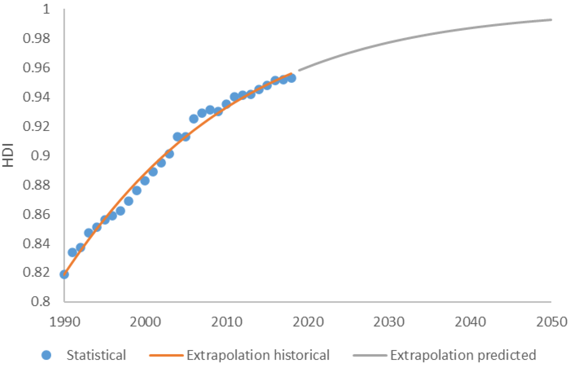
Previous research estimated future per capita food demands on a country level until 2050 based on an exponential relationship between per capita animal product intake and the Human Development Index (HDI) [7]. Here, HDI was extrapolated with a logistic regression based on data from [43]. Logistic regression was chosen because the HDI is bounded to values between 0 and 1 (with 1 being the highest attainable score), with countries with a high HDI evolving more slowly. Further, this asymptotic behavior suggests the existence of smooth development pathways [43]. The logistic regression formula is shown in Equation (4)

$$\mathrm{HDI}=\frac{1}{1+{\mathrm{e}}^{-at+b}}$$

(4)

where t is a year, and a and b are the coefficients to fit available data. In this study, German federal states’ annual HDI values between 1990 and 2017 [44] were used to derive a and b for each federal state. As an example, historical data and extrapolation values from 1990 until 2050 of the whole Germany are shown in Figure 2. For 1990 to 2017, the coefficient of determination $R^2$ between historical and calculated data is 0.99. The HDI of an individual federal state was interpolated to better reflect the local situation.

According to [5], the amount of total calorie demand, animal products, sugar-sweeteners, vegetable oils, and vegetables has an exponential relationship with HDI. The relation between ${\mathrm{c}}_i$, the number of calories per category i [1000 kcal/cap/day], and the HDI can be expressed by Equation (5):

$$\log c_i={\mathrm{c}}_i+{\mathrm{d}}_i\times \mathrm{HDI}$$

(5)

where ${\mathrm{c}}_i$ and ${\mathrm{d}}_i$ are the coefficients per category, whose values are shown in Figure S6 and Table S7. The coefficient of determination $R^2$ between HDI and total food calorie is 0.8, and the $R^2$ between HDI and animal food calorie demand is 0.91 [7].

By combing Equations (4) and (5), a dietary pattern change in terms of food calorie demand for different food categories could be expressed as a function of the year. This is because the $R^2$ values of Equations (4) and (5) show a strong correlation between variables, a reasonably strong linkage between a given year and the food demand pattern change of the existing history. Additionally, the uncertainty of future diet pattern changes, e.g., reduced animal product consumption due to increased awareness on its impact on animal well-being or the climate, was not considered. With enough confidence, we argue that this method can be used to predict food demand change if the future diet pattern follows past developments.

Regarding the population of a given region, population numbers were taken from the statistical census portal for study regions with clear administration boundaries [41]. For regions where population data is not statistically available, e.g., randomly defined regions, the population can be simulated by a previously published method developed for SimStadt that calculates building occupant numbers for residential buildings based on high-resolution statistical census data and a 3D building model [33].

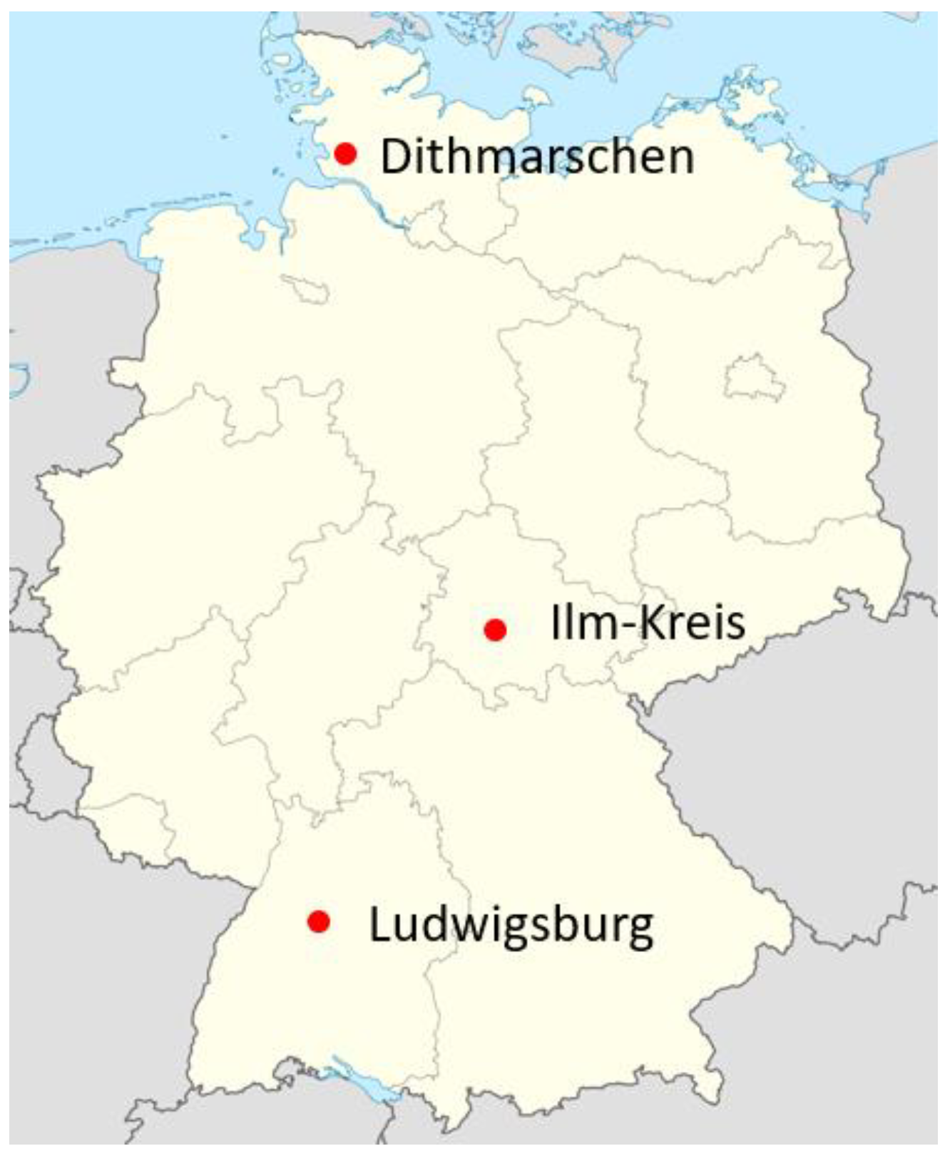
2.3. Case Study Regions

Three case study regions (German “Landkreise” or counties) were chosen for validation as well as sensitivity analysis out of a total of 400 German counties because, firstly, county-wide land use, soil, and crop distribution data are available, secondly, they differ concerning their agricultural land use, and thirdly, they are located in different parts of Germany, with differing climates.

• Sub-urban: Ludwigsburg, Baden-Wuerttemberg, Southern Germany
• Forest dominant: Ilm-Kreis, Thuringia, Mid-Eastern Germany
• Agriculture dominant: Dithmarschen, Schleswig-Holstein, North Germany

The choice of these counties thus reflects the diversity of German and to some extent more broadly typical northern European landscapes.

Table 3. Socio-economic and climatic data of the three German counties used for validation.

Parameter	Unit	Ludwigsburg	Ilm-Kreis	Dithmarschen
Area 1	[km2]	687	805	1428
Population density 2	[Pers./km2]	794	132	93
Agricultural land cover rate 3	[%]	55	45	78
Forest cover rate 3	[%]	18	43	3

^1,2 Federal Statistical Office of Germany [45]; ³ Federal Statistical Office of Germany [46].

provides key characteristics for each county and Figure 3 shows the location of the counties within Germany.

2.4. Validation

2.4.1. Food Demand and Consumption

Table 4. Comparison between simulated per capita food demand and statistical food consumption in the years 2005, 2009, 2013, and 2017.

Year	Mean Body Weight, in kg [38]	Simulated Physical Food Demand with Moderate PAL of the US, in kcal/capita/day	Statistical Food Consumption in, kcal/capita/day [42]	Difference in %
2005	74.9	2387	3450	31%
2009	75.6	2396	3515	32%
2013	76.3	2405	3498	31%
2017	77	2415	3542	32%

illustrates per capita food consumption and demand. As mentioned in Section 2.2, the amount of food consumption, i.e., the amount bought, is typically greater than physical food demand because of waste and storage. Data on food consumption is typically more easily available than the actual physical food demand of inhabitants [42]. Moreover, the food calorie demand method by [9] took the average PAL values of non-overweighted adults in the United States as a moderate PAL, but a PAL was not provided for other countries. Since this paper focused on case studies in Germany, a validation process was executed to improve accuracy by eliminating the errors introduced by food waste, storage, and PAL.

Body weight data and aggregated food demand for Germany are available for the years 2005, 2009, 2013, and 2017 [38,42]. These data were processed and listed in Table 3. As the mean body weight increases, simulated food demand increases in line, from 2387 kcal/capita/day to 2415 kcal/capita/day. Statistical data confirms this trend. However, the differences between simulated food demand and statistical food consumption are 31–32% for all years. This indicates that because of food waste and differences in PAL between Germany and the USA, actual German food consumption is about 31% higher than the simulated DER. Food consumption was thus derived from the physical food demand based on Equation (6).

$$Food consumption=DER\times 1.31$$

(6)

2.4.2. Food Potential

Statistical food calorie potential and demand are only available at the national level. To validate results at a regional level, the crop calorie potentials map (CP) by Pradhan et al. with resolution of 5 arc degrees was adopted [13]. As validation reference, the gridded crop calorie potential map used downscaled data on simulated crop yields and area harvested from GAEZv3.0 for the year 2000 [47], with no more recent updates available. Therefore, GAEZv3.0 estimated crop yields and area harvested in a grid cell for the year 2000 based on FAO agricultural production statistics from the FAO.

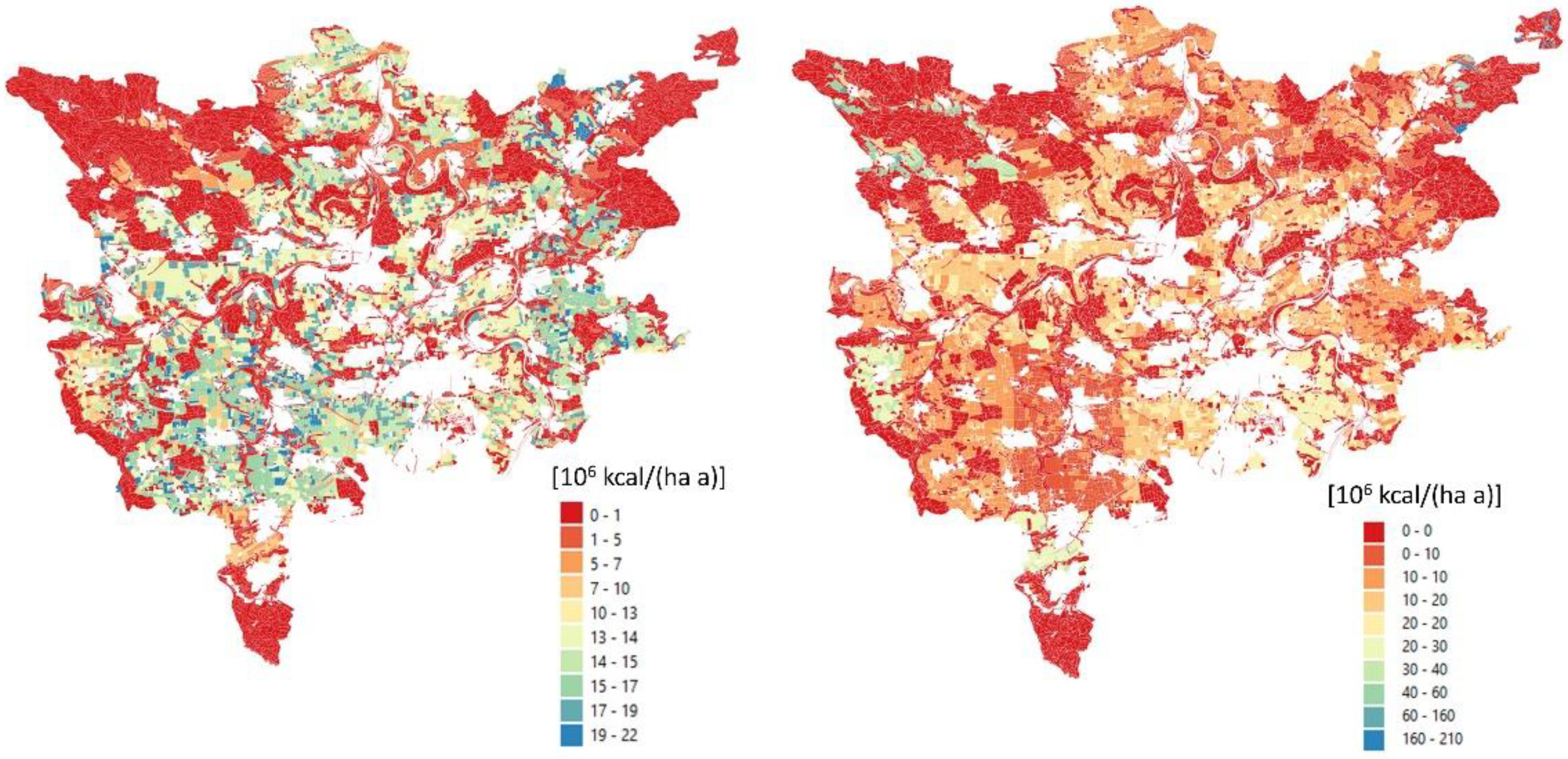
The proposed methodology of food potential simulation was validated in the three case study counties. The crop calorie potentials simulated by SimStadt and by Pradhan and GAEZ as references are listed in

Table 5. Crop calorie potential simulated by SimStadt and by Pradhan and GAEZ.

Parameter	Unit	Ludwigsburg	Ilm-Kreis	Dithmarschen
Crop calorie potential-SimStadt	[106 kcal]	583	477	1255
Crop calorie potential–GAEZ and Pradhan et al.	[106 kcal]	636	470	998
Difference		−7%	1%	26%

. At the county level, the simulated results in our study varied from the results of Pradhan and GAEZ by −7%, 1%, and 26% in Ludwigsburg, Ilm-Kreis, and Dithmarschen, respectively.

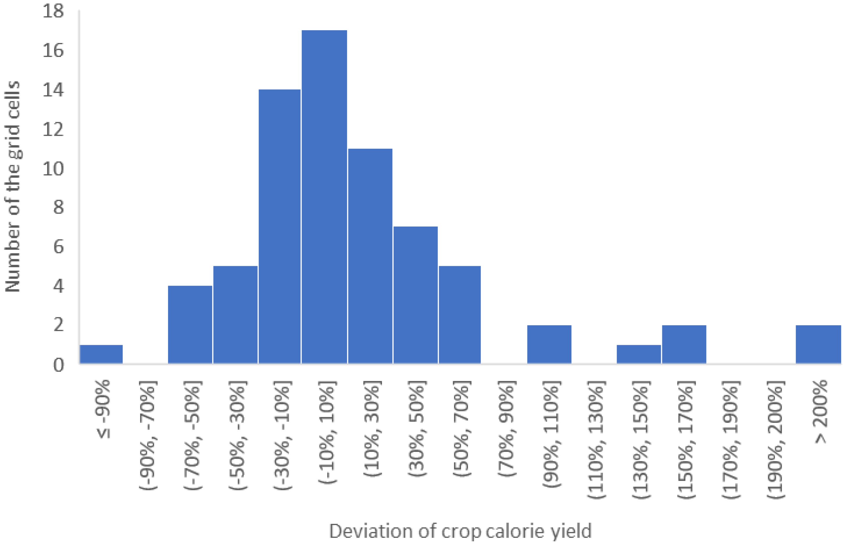
As mentioned in Section 2.1, the crop calorie potential map from Pradhan [13] has a resolution of 5 arc degrees (around 6 km for German latitudes), which typically covers more than 150 land use polygons from the DLM integrated land use map used for crop calorie simulation in SimStadt: as an example, Figure S6 in the supplementary data illustrates grid cells from [13] and land use polygons in Ludwigsburg county. As Figure 4 shows, 70% of the grid cells have a deviation of crop calorie potential between both approaches of −30% and 30%. Large deviations can be due to grid cells not fully within a studied county, and the calorie potential of the grid being concentrated in the area outside the boundary, i.e., the grid cell’s agricultural land lies primarily outside county boundaries and forests or urban areas can be found inside. See for example the grid cells along the left boundary in Figure S6.

2.5. Sensitivity Analysis

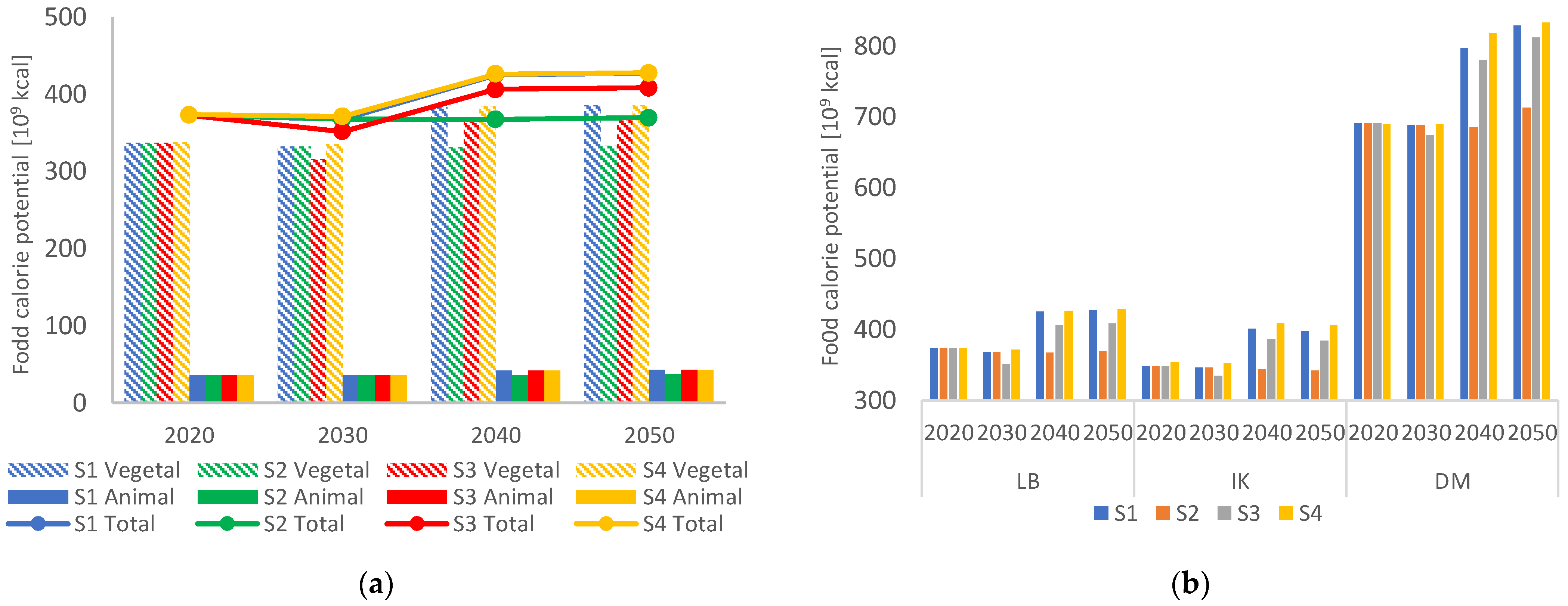
We defined four cases to project food production (S) and three cases to project food consumption (D) from 2020 until 2050. Case S1 is the baseline on the production side, with climate change from 2020 to 2050 as included in Meteonorm data, the share of the organic farming area following historical growth rates, no artificial irrigation, and an energetic use factor of crops of zero after 2030 (Background: With the Renewable Energy Directive 2018/2001 (RED II), adopted in December 2018, the EU (European Union) is continuing to develop the political framework for the use of renewable energy sources in the transport sector for the period from 2021 to 2030 [48], while first-generation bioethanol, i.e., ethanol from crops, will be phased out until 2030). In the case of S2, RED II was not considered, allowing the energetic use of certain crops. This scenario serves as a second base case, since it allows for easier comparison of results before 2030 and afterwards.

In S1, the share of organic farmland in Germany follows historical statistical data [49] as shown in Figure S1, when the ratio increased from 1.6% in 2002 to 9.1% in 2018. In S1, we thus applied a linear fit to the historical trend. The 2050 share of the organic farming area then reaches 16.7%. Organic farming here refers to a sustainable agricultural system respecting the environment and animal welfare, but also includes all other stages of the food supply chain. To assess an organic farming yield in detail as compared to conventional methods, an extensive simulation tool that considers agricultural systems holistically would have been needed [50], which is beyond the scope of this study and the capabilities of the biomass simulation tool [20,51]. However, we examined the relative yield performance of organic and conventional farming systems globally and showed that organic farming land on average had 34% lower yields than conventional approaches in most comparable settings. Since the action plan for the development of EU organic farming aims to have at least 25% of EU agricultural land farmed organically by 2030 [52], case S3 assumed this value for 2030 and followed the same absolute increment percentage as in case S1 between 2030 and 2050. Lastly, case S4 includes artificial irrigation. A crop’s irrigation demand was determined by the minimal amount of external water that has to remain in the root zone throughout the growing cycle so that the given water stress was maintained in the growing season. The higher the water stress level, the lower the amount of water that was allowed to stay in the soil [20].

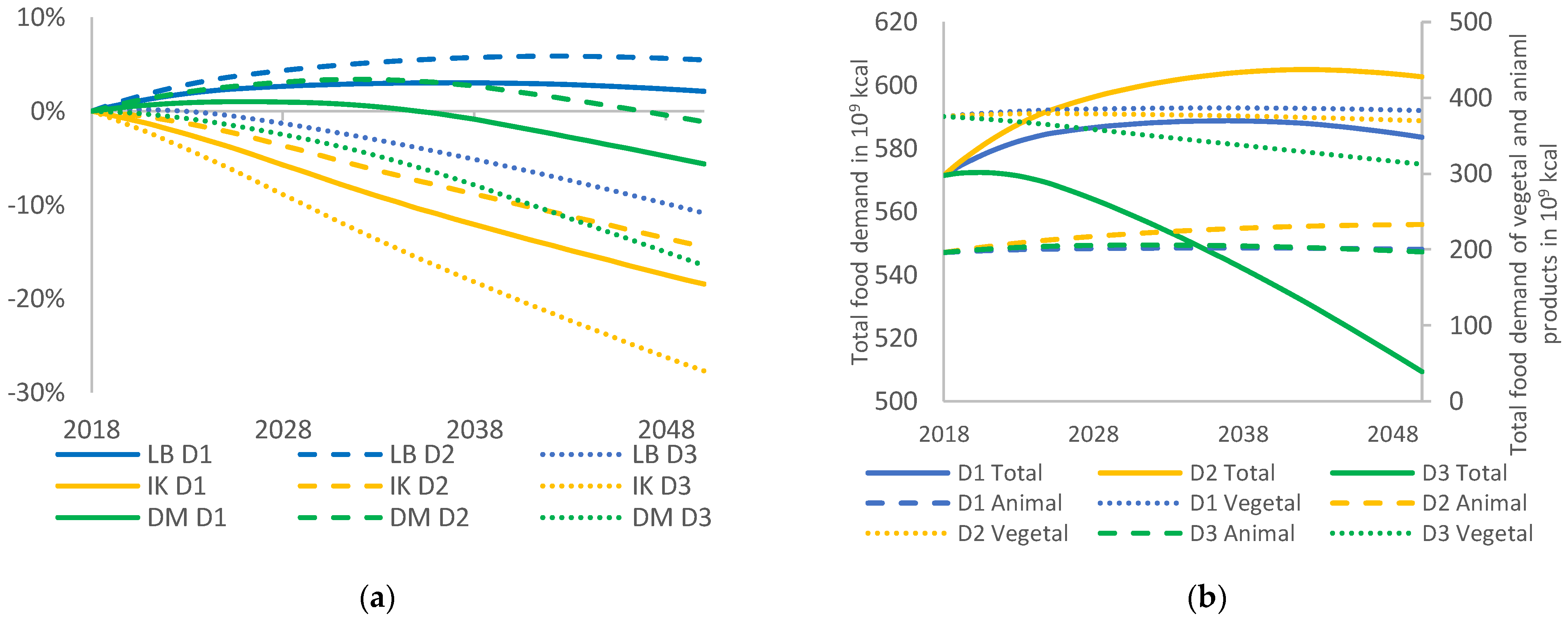
On the food demand side, D1 is the baseline case where the dietary pattern stays the same as in the year 2017, but changes in population change food demands. Population predictions were taken from [53]. In addition to population change, diet changes were considered in D2, with the changes following the extrapolating and prediction method of food demands prediction shown in Section 2.3. In D3, besides the population change and dietary demand change, a lower food waste rate was assumed: the EU and its member countries are committed to meeting the Sustainable Development Goal target to halve per capita food waste at the retail and consumer level by 2030 [54]. Sector 2.3.1 suggested a gap between food consumption, i.e., the number of calories people buy, and DER, i.e., the minimal amount of calories to maintain physical activity, of 31%. Therefore, a smaller gap of 15% was assumed in D3. All cases are summarized in

Table 6. Scenario summaries with key parameter differences.

Case	Case Explanation
S1 (Baseline scenario for food supply)	Predicted future climate from 2020 to 2050 as provided by Meteonorm; energy crop percentage for relevant crops set to 14% from 2020 to 2030 and 0% from 2030 to 2050; share of organic farming follows the linear fitting curve based on historical data from 1994 to 2018
S2	Climate and organic farming area percentages are identical to S1, energy crop percentage stays at 14% after 2030
S3	Climate and energy crop percentage identical to S1, the organic farming area percentage set to 25% in 2030 and follows the same increment trend as in S1
S4	Climate, energy crop percentage, and organic farming area percentage identical to S3. Additional irrigation was added to keep water stress levels at 90%
D1 (Baseline scenario for food demand)	The dietary pattern stays the same as in the year 2017; population change was considered
D2	Dietary pattern changes and population changes were considered at the same time.
D3	Dietary pattern changes and population changes were considered at the same time. Half of the food waste was assumed to be avoided until 2050.

.

3. Results

3.1. Spatial Pattern of Food Potential

Figure 5 shows the vegetal and animal calorie potential density of each land use polygon in Ludwigsburg county. The built-up urban areas, roads, and water bodies are excluded and shown in white. The vegetal calorie potential is directly related to the land use type, as can be seen from the forested areas in the northwest, northeast, and south of the county, which have no food vegetal calorie potential. The high calorie (>15 million kcal/(ha a)) potential areas in green and blue coloring are cultivated with cereal and maize, while land areas with low to middle vegetal calorie potential (4 million kcal/(ha a) to 15 million kcal/(ha a)) are for example vineyards or fruit plantations. Polygons with a high animal potential are usually overlayed with polygons with a high vegetal potential: Figure 5 (right) shows that high animal calorie potential (>330 million kcal/(ha a)) was observed in the northwest of Ludwigsburg where grasslands and forests dominate. As animal feedstock is also imported, animal calorie potential can be higher than the vegetal calorie potential for certain polygons. But in general, the animal product calorie potential is around 10% of the vegetal calorie potential in Ludwigsburg in 2020. Similar results for county Ilm-Kreis and Dithmarschen can be found in Figures S2 and S3 in supplementary data, respectively.

3.2. Development Food Demand until 2050

Figure 6a shows the forecast of total food calorie demands in three study regions. As case D1 only considered population development, the shape of the lines was defined by the population change. Population growth of 3% is expected in Ludwigsburg while Ilm-Kreis faces a net population decrease of 15% until 2050, with the population in Dithmarschen increasing by only 1% until 2050. In case D2, diet pattern changes are included. In our method, food demand follows the same trend as the HDI. Since HDI is expected to be steadily growing until 2050, food demand per capita increases. Compared to D1, total food calorie demand is around 3% more in D2 in 2050. In D1 and D2, a food waste rate of 30% was assumed, as was explained in Sector 2.3.1. If that rate is halved, as assumed in D3, total food demand decreases by 28% in all three case study counties.

Figure 6b shows the forecast based on our simulation of food calorie demands for Ludwigsburg. Total food demand is disaggregated into animal and vegetal food demand. In D1, the ratio between animal and vegetal food demand was kept constant based on 2018 data. The total food calorie demand for 2018 was 571 billion kcal, of which 34% was provided by animals and 66% by vegetal products. D2 indicates the impact of diet pattern change: in 2018, a person statistically consumed 990 kcal of animal products and 1890 kcal of vegetal products per day. The amount of animal product consumption is expected to reach 1150 kcal in 2050, while 2976 kcal less vegetal products are expected to be consumed. Therefore, despite a population growth of 2.1%, 2050 demand for vegetal products in 2050 is 1.5% lower than in 2018, while animal food product demand is expected to grow by 18%. A similar trend is observed in the other two counties, shown in Figures S4 and S5 in Supplementary Data.

3.3. Temporal Development Food Potential

Annual food calorie potential for Ludwigsburg is shown in Figure 7a. Future food calorie potential was simulated for 10-year intervals from 2020 to 2050. The baseline case S1 (blue) shows a 15% increase in annual food potential, from 373 billion kcal/a in 2020 to 428 billion kcal in 2050, mostly due to RED II and its restriction on using farmland exclusively for energy production after 2030. Compared with S1, case S2 (green) assumed that about 15% of farmland can be used for energy crop cultivation [55]. In this case, climate change is the only variable: average yearly temperatures are predicted to increase from 10.2 °C in 2020 to 10.8 °C in 2050, while precipitation slightly increases from 709 mm/a to 715 mm/a. The changing climate harms crop biomass yields, thus reducing calorie yields by 1.5% until 2050 in Ludwigsburg. Case S3 (red) increases the organic farming land share to 25% in 2030, resulting in 4.5% less vegetal calorie yields compared to S1. S4 (yellow) includes artificial irrigation and shows that irrigation increases annual food calorie potential by about 1% at the expense of 4.7 to 7.1 million m³ of water demand, around 1% of Ludwigsburg’s total 2020 demand [56].

Comparing the three counties in Figure 7b shows that Dithmarschen has by far the highest annual food calorie potential of 690 billion kcal, due to having the largest agricultural land area. However, Ludwigsburg had the highest average annual yield density, of 7.4 million kcal per hectare, and Ilm-Kreis the lowest yield density of 4.7 million kcal per hectare and year in 2020. In all three regions, average annual temperatures and annual precipitation are expected to increase until 2050. Case S2 shows the food calorie potential reactions to climate change until 2050. In Ludwigsburg and Ilm-Kreis the climate change is unfavorable for crop production, resulting in a lower food calorie potential with a minor decrease of 1.6%. However, in Dithmarschen the annual food calorie potential is expected to increase by 4% between 2020 and 2050.

Comparing S1 and S4 shows that irrigation increases annual food potential by less than 2% on average. This increased potential is at the expense of between 58 and 680 m³ of irrigation water per hectare and year, as shown in

Table 7. Irrigation water demand density to keep water stress levels in the soil at 90%, in m³ per hectare.

Year	Ludwigsburg	Ilm-Kreis	Dithmarschen
2020	95	680	53
2030	141	403	87
2040	108	189	57
2050	93	253	73

. Due to its relatively dry climate, irrigation water demands in Ilm-Kreis are higher than in other regions to reach the same amount of water amount in the soil (Table S8). Therefore, applying irrigation could improve the food potential by around 2% in Ilm-Kreis compared with less than 1% in other regions. The predicted increment of rainfall reduced the additional irrigation demand from 680 tonness per hectare (the year 2020) to 253 tonness per hectare (the year 2050) in Ilm-Kreis. Dithmarschen required the lowest irrigation density among the three counties because it has the most humid and cool climate of all three counties.

4. Discussion

The methods and tools presented in this paper provide a bottom-up method to simulate the local food potential and demand mainly based on the CityGML geoinformatics data model in one single energy-water-food simulation platform. The presented method provides reasonably accurate results in terms of local food calorie potential. Due to a lack of statistical data on this scale, the method was validated against another model and showed differences in annual food potential of between −7% and 26%. These differences between annual crop calorie potential by the SimStadt-based method presented here and the gridded crop calorie potential by Pradhan et al. and GAEZv3.0 [13] can be due to several methodical differences: (i) GAEZv3.0 took 23 major crop types both for rainfed and irrigated conditions into consideration while our method simulates all the agricultural land only with rainfed conditions; (ii) Pradhan et al. considered 19 food crop types, while only 10 food crop types are simulated in the proposed method because of limitations of applied crop distribution map by [27]. Comparing results for all cells of 5 arc minutes by 5 arc minutes, 70% of the grids had deviations between −30% and 30%.

Restricting land used exclusively for energy crop production (see the change between cases S1 and S2) is the most effective way to increase annual food production potential. Climate change (see the development between 2020 and 2050 in case S2) in contrast generally reduces annual biomass yields by about 2%. However, higher annual average temperature and precipitation in Dithmarschen increased annual food potential by around 4%. In all regions and years, irrigation provided a potential increment of less than 2% (see case S4 compared to case S1) at the expense of irrigation water requirements of between 58 to 680 m³ per hectare and year. It has to be noticed that this method only simulates 10 main crop types, which are representative in bioenergy potential calculations. In reality, local food production varieties alone cannot fulfill people’s food demand, e.g., for exotic fruits. Only land-produced food potential was simulated without considering aquatic products in this study. Therefore, this method is limited to extensive food potential simulation, but its main goal is rather to simulate a relative loss of annual food production potential when using land fields more for energetic purposes, i.e., bioenergy, free land PV, or wind. With the result of this paper, low-yielded land can be identified and potentially converted into PV farms to reach more efficient land use.

The food demand assessments depend on two main parameters: the number of occupants and per capita food demand. A previous study [33] simulated the household and occupants number of each building based on the 3D building CityGML data model and census data. Even though for this study only the total number of residents per county was relevant, it is thus also possible to simulate the food calorie potential of any neighborhood or sub-region, including across administrative boundaries or to-be-built areas where statistical values are not available. The per capita food calorie consumption, including food waste and storage, was estimated based on body weight, age distribution, PAL, and birth rate. Additionally, diet patterns were predicted according to HDI development until 2050. The simulation results show that in the Ludwigsburg region per capita, animal products demand was 990 kcal, and vegetal products demand was 1894 kcal per day in 2018. The amount of animal product consumption is expected to rise by 16% by 2050; meanwhile, 4% fewer vegetal products are expected to be consumed. The food waste by half can compensate for the increase in food demand. However, the food pattern prediction was based on historic data and behaviors. The trend of a vegetarian/vegan diet is not projected in this paper.

In Ludwigsburg, simulated local calorie potential covers 64% of simulated overall food demand, while animal calorie demand can be converted locally by less than 20% (Both with potential case S1 and demand case D2 in year 2020). In Ilm-Kreis and Dithmarschen, the respective ratios are 300/262% and 486/859%, respectively, reflecting the lower population density in Dithmarschen and the forested landscape in Ilm-Kreis. As can be seen from these numbers, and has been investigated in other works [6], a vegetal-oriented diet needs less arable land compared to an animal-oriented diet. Switching to more vegetal diets would thus open up room for higher shares of organic farming with its reduced yields but positive environmental impacts.

5. Conclusions

Every regional food system has connections and impacts other resources, notably water and energy. Due to the complexity of food systems, this study narrows down the notion of food system to food potential and demand. This study addresses the food potential and demand simulation at the regional level in high spatial resolution within a single uniformed simulation platform that already covers energy (roof photovoltaic, heating/electricity demand, bioenergy potential) and water (urban water demand of residential/non-residential buildings, crop water demand). The uniqueness of this method involves shifting the minimal result unit to land use polygon/building. This allows simulation of the food potential of each land field, which might also contain energetic potential in the form of bioenergy, free land PV, and wind. This differentiates this approach from other models and approaches that often focus on a national level. The proposed method thus helps to establish a more integrated planning of energy and water infrastructures in the context of climate change by ensuring that any repercussions in the food sphere are assessed properly. Moreover, basing the method on a generally available geoinformatics input base enables transferability to other regions in Germany and possibly globally, as well as at any regional scale from community to county to federal state.

References

1. Rasul, G. Managing the food, water, and energy nexus for achieving the Sustainable Development Goals in South Asia. Environ. Dev. 2016, 18, 14–25. [Google Scholar] [CrossRef] [Green Version]
2. Obersteiner, M.; Walsh, B.; Frank, S.; Havlík, P.; Cantele, M.; Liu, J.; Palazzo, A.; Herrero, M.; Lu, Y.; Mosnier, A.; et al. Assessing the land resource–food price nexus of the Sustainable Development Goals. Sci. Adv. 2016, 2, e1501499. [Google Scholar] [CrossRef] [Green Version]
3. Ghodsvali, M.; Krishnamurthy, S.; de Vries, B. Review of transdisciplinary approaches to food-water-energy nexus: A guide towards sustainable development. Environ. Sci. Policy 2019, 101, 266–278. [Google Scholar] [CrossRef]
4. Alexander, P.; Brown, C.; Arneth, A.; Finnigan, J.; Moran, D.; Rounsevell, M.D.A. Losses, inefficiencies and waste in the global food system. Agric. Syst. 2017, 153, 190–200. [Google Scholar] [CrossRef] [PubMed]
5. Béné, C.; Fanzo, J.; Prager, P.D.; Harold, A.A.; Mapes, B.R.; Toro, P.A. Camila Bonilla Cedrez. Global drivers of food system (un)sustainability: A multi-country correlation analysis. PLoS ONE 2020, 15, e0231071. [Google Scholar] [CrossRef] [PubMed] [Green Version]
6. Kastner, T.; Rivas, M.J.I.; Koch, W.; Nonhebel, S. Global changes in diets and the consequences for land requirements for food. Proc. Natl. Acad. Sci. USA 2012, 109, 6868–6872. [Google Scholar] [CrossRef] [PubMed] [Green Version]
7. Pradhan, P.; Reusser, D.E.; Kropp, J.P. Embodied greenhouse gas emissions in diets. PLoS ONE 2013, 8, e62228. [Google Scholar] [CrossRef] [Green Version]
8. Pradhan, P.; Kriewald, S.; Costa, L.; Rybski, D.; Benton, T.G.; Fischer, G.; Kropp, J.P. Urban Food Systems: How Regionalization Can Contribute to Climate Change Mitigation. Environ. Sci. Technol. 2020, 54, 10551–10560. [Google Scholar] [CrossRef]
9. Hiç, C.; Pradhan, P.; Rybski, D.; Kropp, J.P. Food Surplus and Its Climate Burdens. Environ. Sci. Technol. 2016, 50, 4269–4277. [Google Scholar] [CrossRef] [Green Version]
10. Khushi, S.; Ahmad, S.R.; Ashraf, A.; Imran, M. Spatially analyzing food consumption inequalities using GIS with disaggregated data from Punjab, Pakistan. Food Sec. 2020, 12, 1283–1298. [Google Scholar] [CrossRef]
11. Beltran-Peña, A.; Rosa, L.; D’Odorico, P. Global food self-sufficiency in the 21st century under sustainable intensification of agriculture. Environ. Res. Lett. 2020, 15, 95004. [Google Scholar] [CrossRef]
12. Haase, M.; Rösch, C.; Ketzer, D. GIS-based assessment of sustainable crop residue potentials in European regions. Biomass Bioenergy 2016, 86, 156–171. [Google Scholar] [CrossRef]
13. Pradhan, P.; Lüdeke, M.K.B.; Reusser, D.E.; Kropp, J.P. Embodied crop calories in animal products. Environ. Res. Lett. 2013, 8, 44044. [Google Scholar] [CrossRef] [Green Version]
14. Rosenberg, D.E.; Tarawneh, T.; Abdel-Khaleq, R.; Lund, J.R. Modeling integrated water user decisions in intermittent supply systems. Water Resour. Res. 2007, 43. [Google Scholar] [CrossRef]
15. Merem, E.C.; Twumasi, Y.; Wesley, J.; Alsarari, M.; Fageir, S.; Crisler, M.; Romorno, C.; Olagbegi, D.; Hines, A.; Ochai, G.S.; et al. Regional Assessment of the Food Security Situation in West Africa with GIS. Food Public Health 2019, 9, 60–77. [Google Scholar] [CrossRef]
16. Nouvel, R.; Brassel, K.-H.; Bruse, M.; Duminil, E.; Coors, V.; Eicker, U. SimStadt, a new workflow-driven urban energy simulation platform for CityGML city models. In Proceedings of the International Conference CISBAT 2015 Future Buildings and Districts Sustainability from Nano to Urban Scale. No. CONF. LESO-PB, EPFL, Lausanne, Switzerland, 9–11 September 2015. [Google Scholar]
17. Weiler, V.; Stave, J.; Eicker, U. Renewable Energy Generation Scenarios Using 3D Urban Modeling Tools—Methodology for Heat Pump and Co-Generation Systems with Case Study Application. Energies 2019, 12, 403. [Google Scholar] [CrossRef] [Green Version]
18. Köhler, S. Stochastic Generation of Household Electricity Load Profiles in 15-minute Resolution on Building Level for Whole City Quarters. In Proceedings of the 16th IAEE European Conference: Energy Challenges for the Next Decade, Ljubljana, Slovenia, 25–28 August 2019. [Google Scholar]
19. Bao, K.; Padsala, R.; Thrän, D.; Schröter, B. Urban Water Demand Simulation in Residential and Non-Residential Buildings Based on a CityGML Data Model. ISPRS Int. J. Geo-Inf. 2020, 9, 642. [Google Scholar] [CrossRef]
20. Bao, K.; Padsala, R.; Coors, V.; Thrän, D.; Schröter, B. A Method for Assessing Regional Bioenergy Potentials Based on GIS Data and a Dynamic Yield Simulation Model. Energies 2020, 13, 6488. [Google Scholar] [CrossRef]
21. Nouvel, R.; Zirak, M.; Coors, V.; Eicker, U. The influence of data quality on urban heating demand modeling using 3D city models. Comput. Environ. Urban. Syst. 2017, 64, 68–80. [Google Scholar] [CrossRef]
22. Zirak, M.; Weiler, V.; Hein, M.; Eicker, U. Urban models enrichment for energy applications: Challenges in energy simulation using different data sources for building age information. Energy 2020, 190, 116292. [Google Scholar] [CrossRef]
23. Bao, K.; Padsala, R.; Coors, V.; Thrän, D.; Schröter, B. GIS-Based Assessment of Regional Biomass Potentials at the Example of Two Counties in Germany. In Proceedings of the 28th European Biomass Conference and Exhibition Proceedings, Marseille, France, 28–30 April 2020; pp. 77–85. [Google Scholar] [CrossRef]
24. Braun, R.; Weiler, V.; Zirak, M.; Dobisch, L.; Coors, V.; Eicker, U. Using 3D CityGML Models for Building Simulation Applications at District Level. In Proceedings of the 2018 IEEE International Conference on Engineering, Technology and Innovation (ICE/ITMC), Stuttgart, Germany, 17–20 June 2018; pp. 1–8. [Google Scholar]
25. Introductin AquaCrop, Food and Agriculture Organization of the United Nations. 2016. Available online: http://www.fao.org/3/i6321e/i6321e.pdf (accessed on 15 January 2021).
26. Arbeitsgemeinschaft der Vermessungsverwaltungen der Länder der Bundesrepublik Deutschland. Digitales Basis-Landschaftsmodell (Basis-DLM). Available online: http://www.adv-online.de/AdV-Produkte/Geotopographie/Digitale-Landschaftsmodelle/Basis-DLM/ (accessed on 10 November 2020).
27. Griffiths, P.; Nendel, C.; Hostert, P. Intra-annual reflectance composites from Sentinel-2 and Landsat for national-scale crop and land cover mapping. Remote Sens. Environ. 2019, 220, 135–151. [Google Scholar] [CrossRef]
28. Wyland, L.J.; Jackson, L.E.; Chaney, W.E.; Klonsky, K.; Koike, S.T.; Kimple, B. Winter cover crops in a vegetable cropping system: Impacts on nitrate leaching, soil water, crop yield, pests and management costs. Agric. Ecosyst. Environ. 1996, 59, 1–17. [Google Scholar] [CrossRef]
29. FAO. Food Balance Sheets: A Handbook; FAO: Rome, Italy, 2001. [Google Scholar]
30. Gustavsson, J.; Cederberg, C.; Sonesson, U.; van Otterdijk, R.; Meybeck, A. Global Food Losses and Food Waste; FAO: Rome, Italy, 2011. [Google Scholar]
31. Bundesanstalt für Geowissenschaften und Rohstoffe. Karte der Bodenarten in Oberböden 1:1.000.000 (BOART1000OB). Available online: https://www.bgr.bund.de/DE/Themen/Boden/Informationsgrundlagen/Bodenkundliche_Karten_Datenbanken/Themenkarten/BOART1000OB/boart1000ob_node.html (accessed on 24 September 2020).
32. Meteonorm. Available online: https://meteonorm.com/en/ (accessed on 12 August 2020).
33. Köhler, S.; Betz, M.; Bao, K.; Weiler, V.; Schröter, B. Determination of household area and number of occupants for residential buildings based on census data and 3D CityGML building models for entire municipalities in Germany. In Proceedings of the Building. Simulation Conference 2021, Bruges, Belgium, 1–3 September 2021. [Google Scholar]
34. Kaltschmitt, M.; Hans, H.; Hofbauer, H. Energie aus Biomasse: Grundlagen, Techniken und Verfahren; Springer: Berlin/Heidelberg, Germany, 2016. [Google Scholar]
35. Bouwman, A.F.; van der Hoek, K.W.; Eickhout, B.; Soenario, I. Exploring changes in world ruminant production systems. Agric. Syst. 2005, 84, 121–153. [Google Scholar] [CrossRef]
36. United Nations University; World Health Organization. Human Energy Requirements. In Proceedings of the Report of a Joint FAO/WHO/UNU Expert Consultation, Rome, Italy, 17–24 October 2001; FAO: Rome, Italy, 2004. ISBN 9251052123. [Google Scholar]
37. Schofield, W.N. Predicting basal metabolic rate, new standards and review of previous work. Hum. Nutr. Clin. Nutr. 1985, 39 (Suppl. S1), 5–41. [Google Scholar] [PubMed]
38. Statistisches Bundesamt. Mikrozensus—Fragen zur Gesundheit. 2005, 2009, 2013, 2017. Available online: https://www.destatis.de (accessed on 16 January 2021).
39. Statistisches Bundesamt. Vorausberechneter Bevölkerungsstand: Bundesländer, Stichtag, Varianten der Bevölkerungsvorausberechnung. Available online: https://www-genesis.destatis.de/genesis/online (accessed on 15 January 2021).
40. Statista. Zusammengefasste Geburtenziffer—Anzahl der Kinder pro Frau in Deutschland nach Bundesländern. Available online: https://de.statista.com/statistik/daten/studie/76262/umfrage/geburtenziffer---anzahl-der-kinder-pro-frau-2007-und-2008/ (accessed on 12 February 2021).
41. Statistisches Bundesamt. Population Depending on Sex and Age (Five Years Age Groups): Census from the Adjusted Stock of Registers. Available online: https://ergebnisse.zensus2011.de/ (accessed on 13 January 2021).
42. FAO. FAOSTAT: FAO Statistical Databases: New Food Balance. Available online: http://www.fao.org/faostat/en/ (accessed on 15 January 2021).
43. Costa, L.; Rybski, D.; Kropp, J.P. A Human Development Framework for CO2 Reductions. PLoS ONE 2011, 6, e29262. [Google Scholar] [CrossRef] [Green Version]
44. HDRO (Human Development Report Office) United Nations Development Programme. Human Development Report 2018: Human Development Indices and Indicators. Available online: http://hdr.undp.org/sites/default/files/2018_human_development_statistical_update.pdf (accessed on 16 January 2021).
45. Statistisches Bundesamt. Daten aus dem Gemeindeverzeichnis: Kreisfreie Städte und Landkreise nach Fläche, Bevölkerung und Bevölkerungsdichte. Available online: https://www.destatis.de/DE/Themen/Laender-Regionen/Regionales/Gemeindeverzeichnis/Administrativ/04-kreise.html (accessed on 3 January 2021).
46. Statistisches Bundesamt. Anbauflächen, Hektarerträge und Erntemengen ausgewählter Anbaukulturen im Zeitvergleich: Hektarerträge ausgewählter Anbaukulturen im Zeitvergleich. Available online: https://www.destatis.de/DE/Themen/Branchen-Unternehmen/Landwirtschaft-Forstwirtschaft-Fischerei/Feldfruechte-Gruenland/Tabellen/liste-feldfruechte-zeitreihe.html (accessed on 16 January 2021).
47. Fischer, G.; Nachtergaele, F.O.; Prieler, S.; Teixeira, E.; Toth, G.; van Velthuizen, H.; Verelst, L.; Wiberg, D. Global Agro-Ecological Zones (GAEZ v3.0)-Model. Documentation; IIASA: Laxenburg, Austria; FAO: Rome, Italy, 2012. [Google Scholar]
48. Directive (EU) 2018/2001: On the Promotion of the Use of Energy from Renewable Sources; European Parliament and of the Council: Strasbourg, France, 2018.
49. Eurostat. Share of Organic Crop Area Out of the Total Utilised Agricultural Area (UAA). Available online: https://ec.europa.eu/eurostat/databrowser/ (accessed on 20 January 2021).
50. Kaufmann, P.; Stagl, S.; Franks, D.W. Simulating the diffusion of organic farming practices in two New EU Member States. Ecol. Econ. 2009, 68, 2580–2593. [Google Scholar] [CrossRef]
51. Seufert, V.; Ramankutty, N.; Foley, J.A. Comparing the yields of organic and conventional agriculture. Nature 2012, 485, 229–232. [Google Scholar] [CrossRef] [PubMed]
52. European Commission. Organic Farming—Action Plan for the Development of EU Organic Production. Available online: https://ec.europa.eu/info/law/better-regulation/have-your-say/initiatives/12555-Organic-farming-action-plan-for-the-development-of-EU-org (accessed on 20 January 2021).
53. Eurostat. Population on 1st January by Age, Sex and Type of Projection. Available online: https://ec.europa.eu/eurostat/databrowser/view/proj_19np/ (accessed on 1 January 2021).
54. European Commission. EU Actions against Food Waste. Available online: https://ec.europa.eu/food/safety/food_waste/eu_actions_en (accessed on 26 January 2021).
55. Fachagentur Nachwachsende Rohstoffe e. V. Anbau und Verwendung Nachwachsender Rohstoffe in Deutschland. FNR. 2019. Available online: https://www.weltagrarbericht.de/fileadmin/files/weltagrarbericht/Weltagrarbericht/16AgrarspritBioenergie/FNR2019.pdf (accessed on 4 October 2020).
56. Öffentliche Wasserversorgung—Statistisches Landesamt Baden-Württemberg. Available online: https://www.statistik-bw.de/Umwelt/Wasser/22025035.tab?R=KR118 (accessed on 17 August 2020).
Figure 1. Flow chart diagram of inputs, models, and output of the methods presented in this paper. The data blocks with a yellow background are the inputs, and the ones with a blue background are the output.
Land 10 00880 g001
Figure 2. An example of HDI in Germany: historical data from 1990 to 2017 (blue), a fit curve of historical data (1990 to 2017, orange), and a fit and extrapolation for 2018 to 2050 (gray).
Land 10 00880 g002
Figure 3. Location of case study regions in Germany.
Land 10 00880 g003
Figure 4. Histogram of deviations of results from SimStadt and GAEZ and Pradhan et al. The y-axis gives the number of grid cells within a deviation range as given on the x-axis.
Land 10 00880 g004
Figure 5. Vegetal (left) and animal calorie potential (right) in Ludwigsburg.
Land 10 00880 g005
Figure 6. (a) Total food calorie demand in the three study regions for the period 2018 to 2050. The relative percentage value shows the change compared to 2018. Ludwigsburg (LB) in blue, Ilm-Kreis (IK) in orange, Dithmarschen (DM) in green; Case D1 in solid line, case D2 in dashed line, case D3 in dotted line; (b) Forecast of total food demand (solid line), vegetal food demand (dotted line), and animal food demand (dashed line) in Ludwigsburg county, 2018 to 2050.
Land 10 00880 g006
Figure 7. (a) Prediction of food calorie potential (solid lines), vegetal food potential (shadowed bars), and animal food potential (solid bars) in Ludwigsburg, 2020 to 2050; (b) Prediction of total food potential in Ludwigsburg (LB), Ilm-Kreis (IK) and Dithmarschen (DM) for four cases, 2020 to 2050.
Land 10 00880 g007