
Relationship of Ecosystem Services in the Beijing–Tianjin–Hebei Region Based on the Production Possibility Frontier


 ,
,
Abstract
:1. Introduction
2. Data and Methods
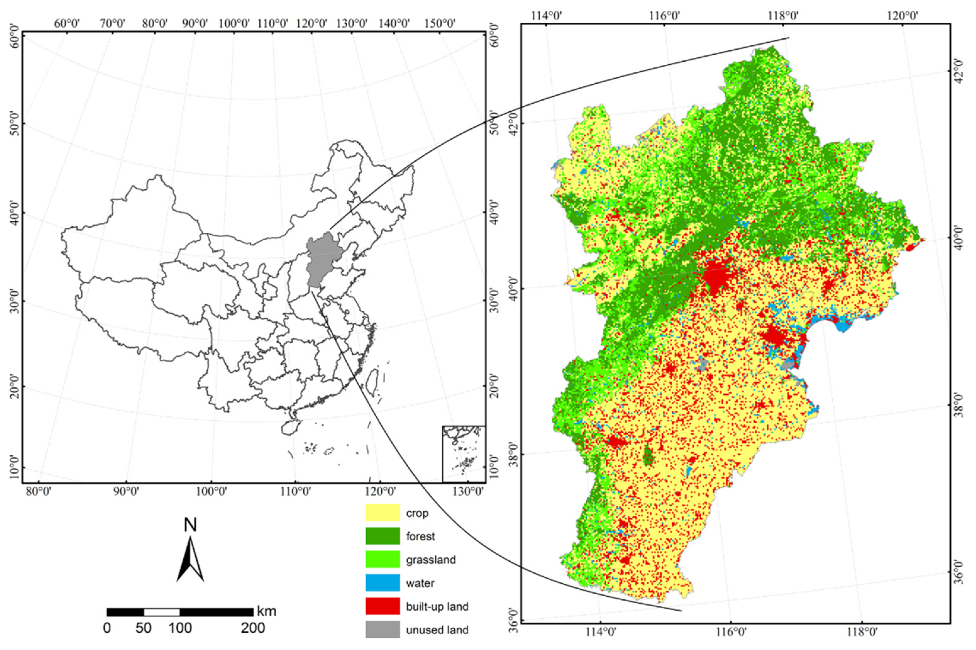
2.1. Study Area
2.2. Data Sources
2.3. Method
2.3.1. Scenario Simulation
2.3.2. Water Yield
2.3.3. Soil Conservation
2.3.4. Carbon Storage
2.4. Plotting the PPF Curve
3. Results and Analysis
3.1. Analysis of Land-Use Simulation Results under Different Scenarios
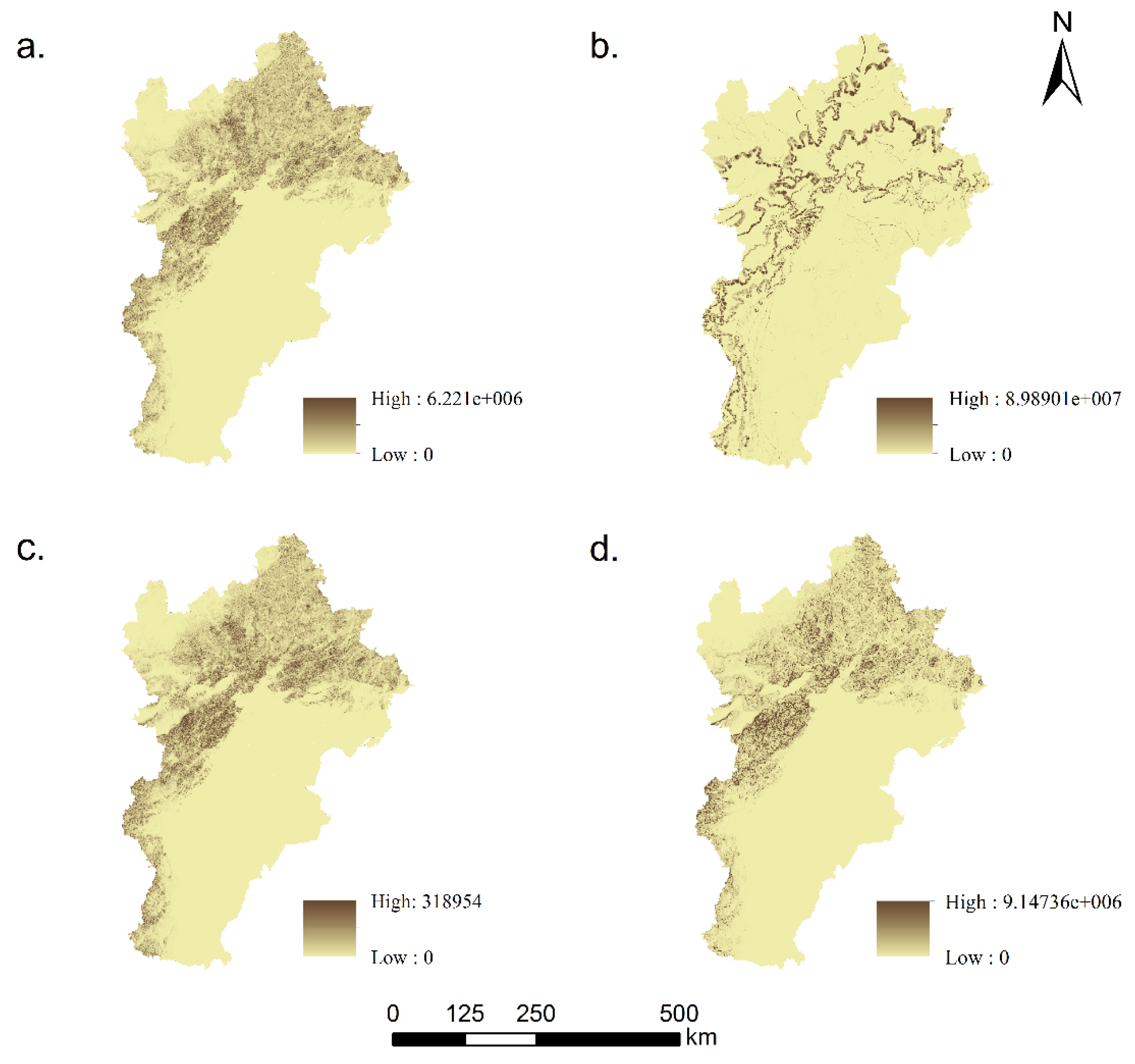
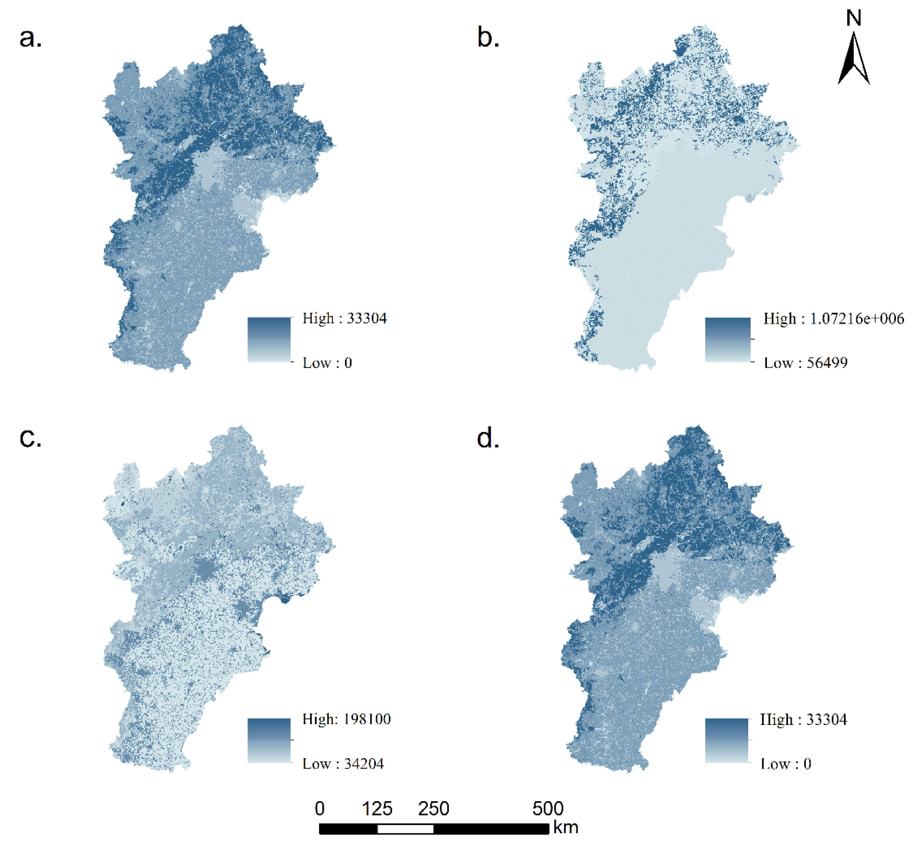
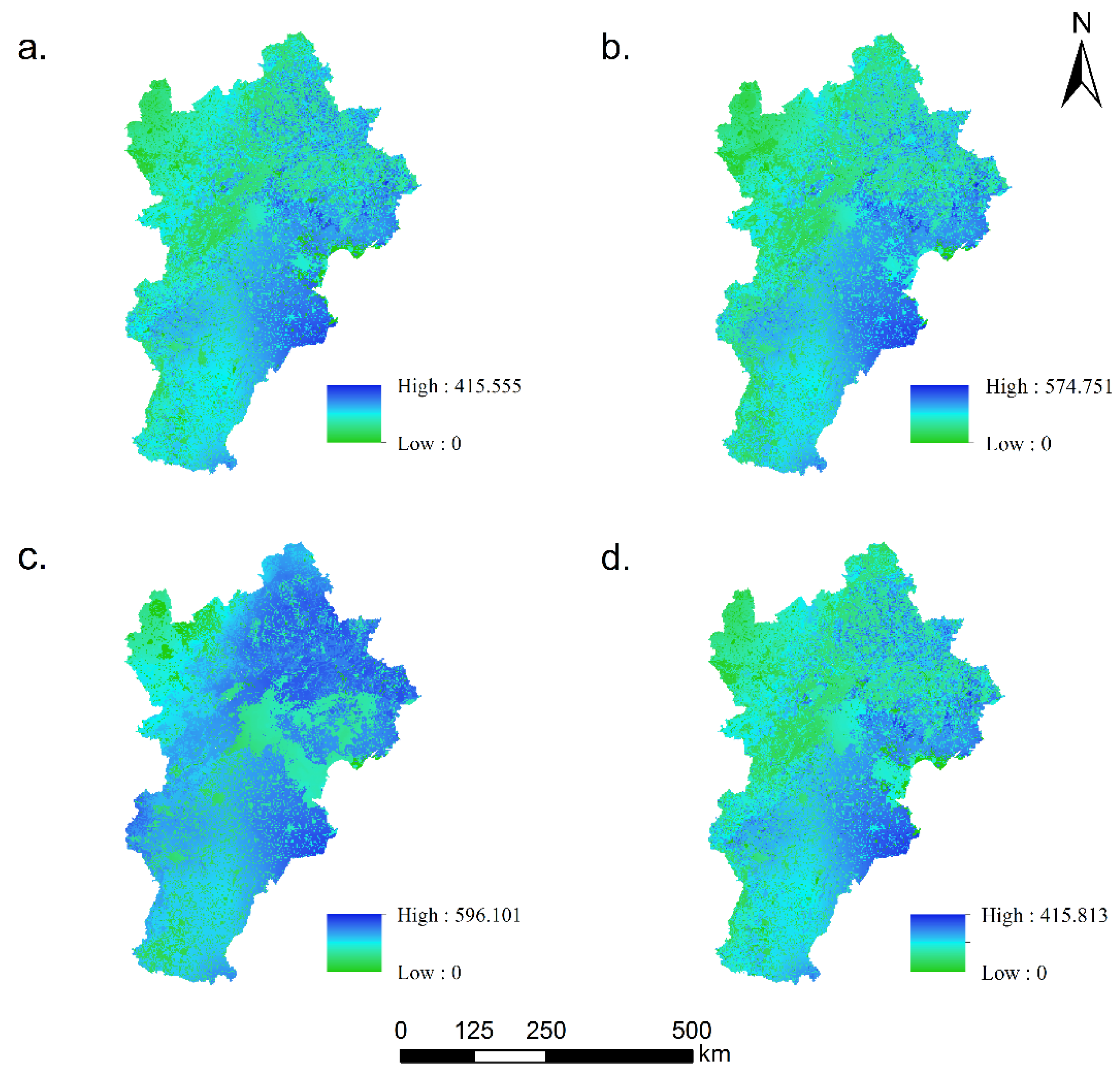
3.2. Spatial Distribution of Ecosystem Services
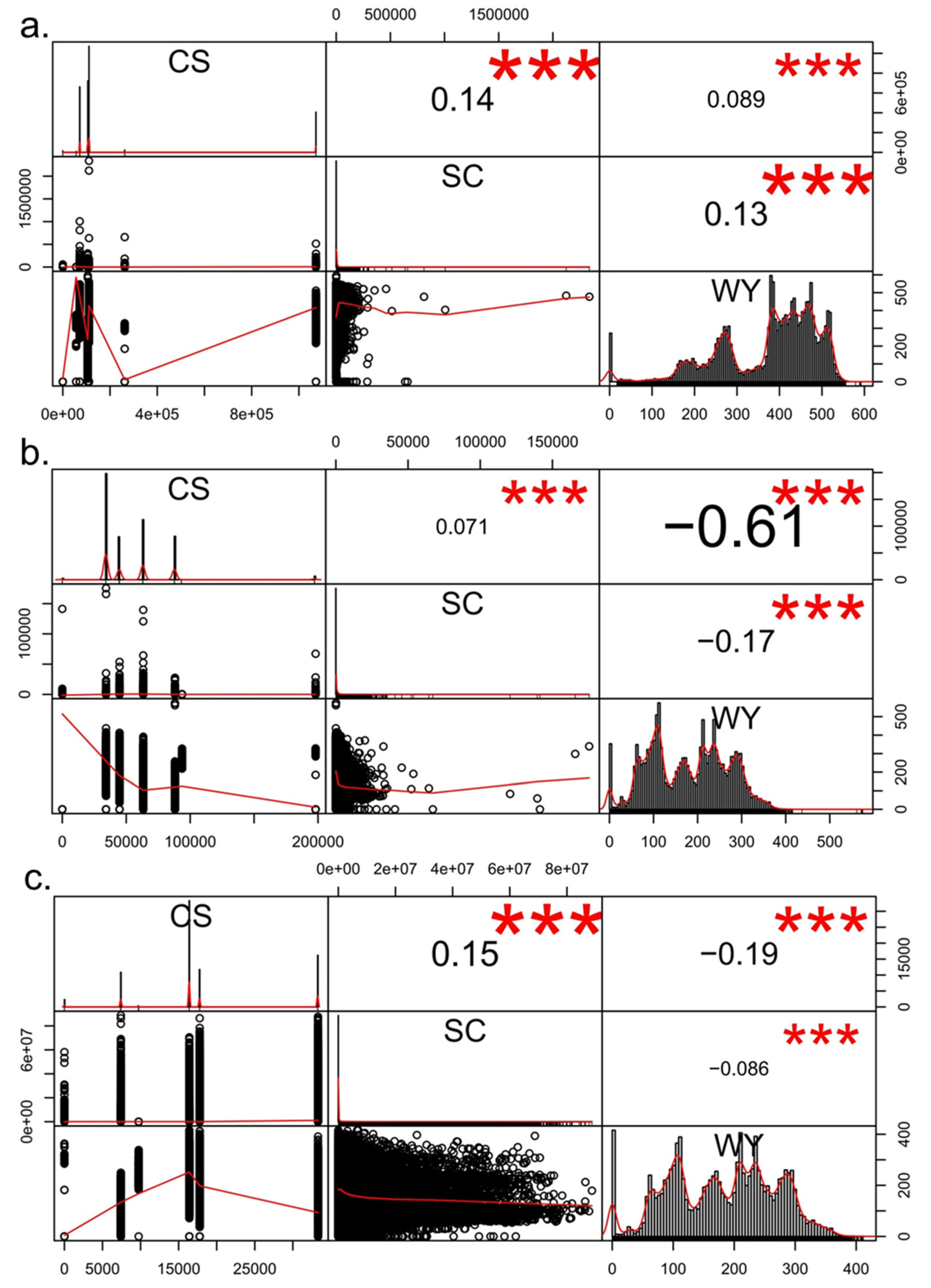
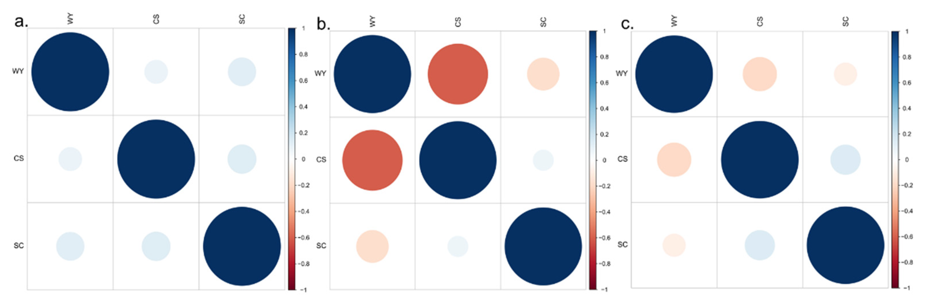
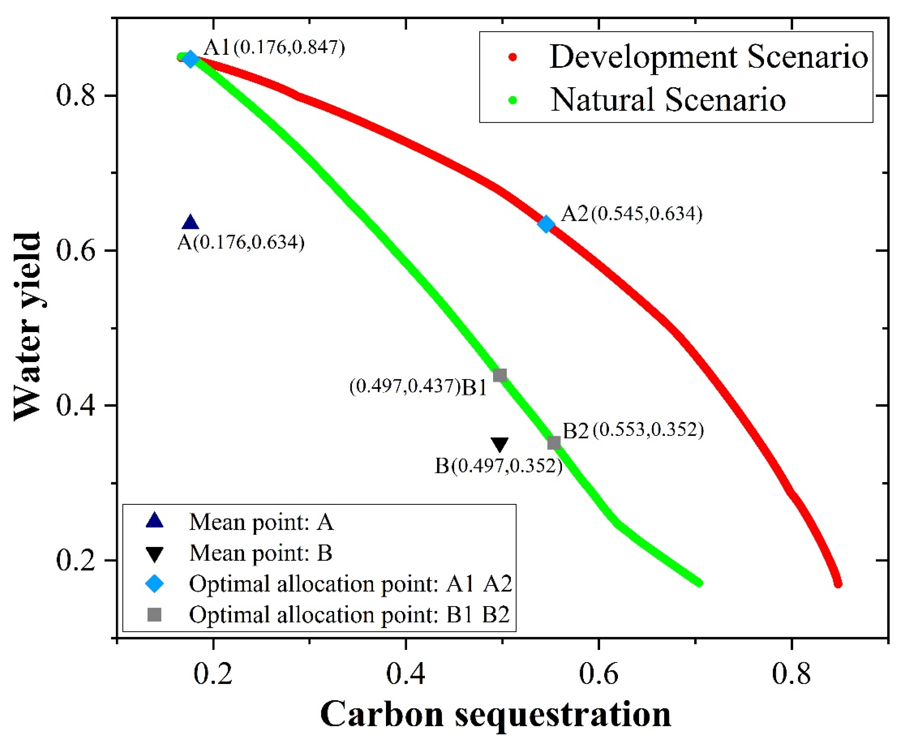
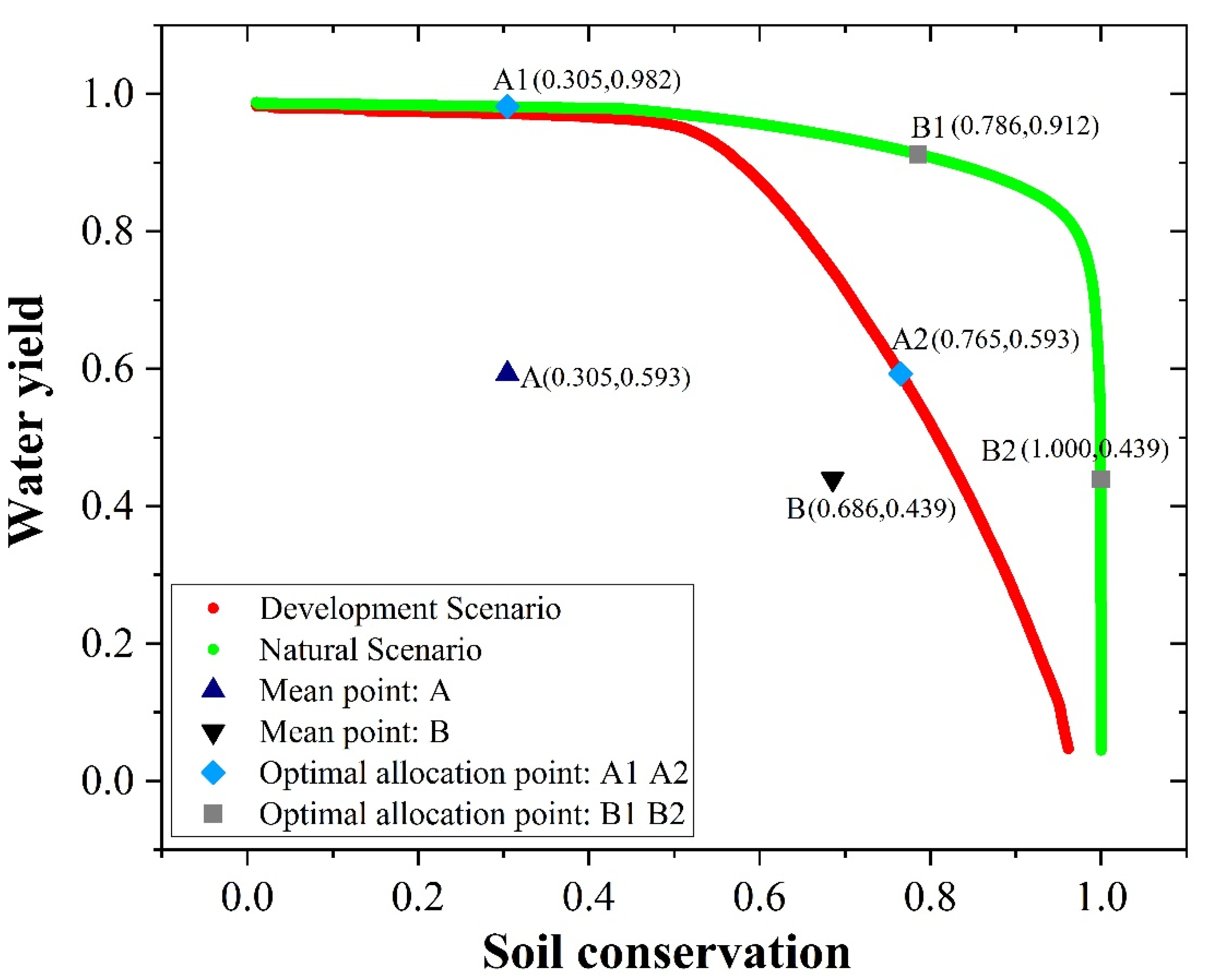
3.3. Ecosystem Service Trade-Off Relationships
3.4. Ecosystem Service Trade-Off Strength and Optimal Allocation
4. Discussion
5. Conclusions
- (1)
- Under the development scenario in 2035, the sprawl of urbanized land in the Beijing–Tianjin–Hebei region will accelerate. This expansion will lead to the occupation of a large amount of arable land and woodland, which is not conducive to the construction of ecological civilization and the sustainable and healthy development of cities in the future. Hence, experts need to plan and control the conversion of a certain amount of arable land and woodland into built-up land.
- (2)
- A trade-off relationship exists between water yield and soil conservation and between water yield and carbon storage services under development and natural scenarios. Synergistic relationships exist among ecosystem services under the conservation scenario. In addition, the trade-off and synergy relationships can be transformed under different land-use scenarios.
- (3)
- In this study, the conservation scenario was found to have the highest value of carbon storage and soil conservation, and the water yield was also at a high level. Wood-land is an important supply area for carbon storage. It has high soil and water conservation capacity. Hence, appropriate measures should be implemented to improve the soil and water conservation function in the region while enhancing the value of ecosystem services by returning the land to the forest to a certain extent.
- (4)
- The PPF curves between ecosystem services under different scenarios in 2035 were plotted, and the trade-off intensity of ecosystem services was calculated. In particular, visual representation of the results of agricultural planning decisions through PPF can help guide the direction of subsequent interdisciplinary research and policy. The findings showed that by controlling the conversion of land-use types, the planning goals of ecological service functions can be achieved. This work provides an important theoretical basis for the sustainable development of land resources in the Beijing–Tianjin–Hebei region.
Author Contributions
Funding
Data Availability Statement
Conflicts of Interest
References
- Bennett, E.M.; Peterson, G.D.; Gordon, L.J. Understanding relationships among multiple ecosystem services. Ecol. Lett. 2009, 12, 1394–1404. [Google Scholar] [CrossRef] [PubMed]
- Mononen, L.; Auvinen, A.P.; Ahokumpu, A.L.; Ronka, M.; Aarras, N.; Tolvanen, H.; Kamppinen, M.; Viirret, E.; Kumpula, T.; Vihervaara, P. National ecosystem service indicators: Measures of social–ecological sustainability. Ecol. Indic. 2014, 61, 27–37. [Google Scholar] [CrossRef]
- Costanza, R.; D’Arge, R.; Groot, R.D.; Farber, S.; Grasso, M.; Hannon, B.; Limburg, K.; Naeem, S.; O’Neill, R.V.; Paruelo, J.; et al. The value of the world’s ecosystem services and natural capital. Ecol. Econ. 1997, 25, 3–15. [Google Scholar] [CrossRef]
- Galic, N.; Salice, C.J.; Birnir, B.; Bruins, R.J.F.; Ducrot, V.; Jager, H.I.; Kanarek, A.; Pastorok, R.; Rebarber, R.; Thorbek, P.; et al. Predicting impacts of chemicals from organisms to ecosystem service delivery: A case study of insecticide impacts on a freshwater lake. Sci. Total Environ. 2019, 682, 426–436. [Google Scholar] [CrossRef] [Green Version]
- Corvalan, C.; Hales, S.; McMichael, A.J.; Butler, C.; McMichael, A. Ecosystems and Human Well-Being: Health Synthesis; World Health Organization: Geneva, Switherland, 2005; Volume 34, p. 534. [Google Scholar]
- Haines-Young, R.; Potschin-Young, M.B. Revision of the Common International Classification for Ecosystem Services (CICES V5.1): A Policy Brief. One Ecosyst. 2018, 3, e27108. [Google Scholar] [CrossRef]
- Kaval, P. Integrated catchment management and ecosystem services: A twenty-five year overview. Ecosyst. Serv. 2019, 37. [Google Scholar] [CrossRef]
- Fisher, B.; Turner, R.K.; Morling, P. Defining and classifying ecosystem services for decision making. Ecol. Econ. 2009, 68, 643–653. [Google Scholar] [CrossRef] [Green Version]
- Ouyang, Z.; Zheng, H.; Xiao, Y.; Polasky, S.; Liu, J.; Xu, W.; Wang, Q.; Zhang, L.; Xiao, Y.; Rao, E.; et al. Improvements in ecosystem services from investments in natural capital. Science 2016, 352, 1455–1459. [Google Scholar] [CrossRef] [PubMed]
- Li, S.; Li, X.; Dou, H.; Dang, D.; Gong, J. Integrating constraint effects among ecosystem services and drivers on seasonal scales into management practices. Ecol. Indic. 2021, 125, 107425. [Google Scholar] [CrossRef]
- Hao, R.; Yu, D.; Liu, Y.; Yang, L.; Qiao, J.; Wang, X.; Du, J. Impacts of changes in climate and landscape pattern on ecosystem services. Sci. Total Environ. 2017, 579, 718–728. [Google Scholar] [CrossRef]
- Cao, Y.; Cao, Y.; Li, G.; Tian, Y.; Fang, X.; Li, Y.; Tan, Y. Linking ecosystem services trade-offs, bundles and hotspot identification with cropland management in the coastal Hangzhou Bay area of China. Land Use Policy 2020, 97, 104689. [Google Scholar] [CrossRef]
- Xu, S.; Liu, Y.; Wang, X.; Zhang, G. Scale effect on spatial patterns of ecosystem services and associations among them in semi-arid area: A case study in Ningxia Hui Autonomous Region, China. Sci. Total Environ. 2017, 598, 297–306. [Google Scholar] [CrossRef] [PubMed]
- Shen, j.; Li, S.; Liu, L.; Liang, Z.; Wang, Y.; Wang, H.; Wu, S. Uncovering the relationships between ecosystem services and social-ecological drivers at different spatial scales in the Beijing-Tianjin-Hebei region. J. Clean. Prod. 2020, 290, 125193. [Google Scholar] [CrossRef]
- Loomes, R.; O’Neill, K. Nature’s Services: Societal Dependence on Natural Ecosystems. Pac. Conserv. Biol. 1997, 6, 220–221. [Google Scholar] [CrossRef] [Green Version]
- Haines-Young, R.; Potschin, M.; Kienast, F. Indicators of ecosystem service potential at European scales: Mapping marginal changes and trade-offs. Ecol. Indic. 2012, 21, 39–53. [Google Scholar] [CrossRef]
- Willemen, L.; Hein, L.; Mensvoort, M.E.F.; Verburg, P.H. Space for people, plants, and livestock? Quantifying interactions among multiple landscape functions in a Dutch rural region. Ecol. Indic. 2010, 10, 62–73. [Google Scholar] [CrossRef]
- Tallis, H.; Kareiva, P.; Marvier, M.; Chang, A. Ecosystem Services Special Feature: An ecosystem services framework to support both practical conservation and economic development. Proc. Natl. Acad. Sci. USA 2008, 105, 9457–9464. [Google Scholar] [CrossRef] [PubMed] [Green Version]
- Howe, C.; Suich, H.; Vira, B.; Mace, G.M. Creating win-wins from trade-offs? Ecosystem services for human well-being: A meta-analysis of ecosystem service trade-offs and synergies in the real world. Glob. Environ. Chang. 2014, 28, 263–275. [Google Scholar] [CrossRef] [Green Version]
- Yang, W.; Jin, Y.; Sun, T.; Yang, Z.; Cai, Y.; Yi, Y. Trade-offs among ecosystem services in coastal wetlands under the effects of reclamation activities. Ecol. Indic. 2018, 92, 354–366. [Google Scholar] [CrossRef]
- Zhong, L.; Wang, J.; Zhang, X.; Ying, L. Effects of agricultural land consolidation on ecosystem services: Trade-offs and synergies. J. Clean. Prod. 2020, 264, 121412. [Google Scholar] [CrossRef]
- Li, B.; Chen, N.; Wang, Y.; Wang, W. Spatio-temporal quantification of the trade-offs and synergies among ecosystem services based on grid-cells: A case study of Guanzhong Basin, NW China. Ecol. Indic. 2018, 94, 246–253. [Google Scholar] [CrossRef]
- Zavalloni, M.; Groeneveld, R.A.; Zwieten, P.V. The role of spatial information in the preservation of the shrimp nursery function of mangroves: A spatially explicit bio-economic model for the assessment of land use trade-offs. J. Environ. Manag. 2014, 143, 17–25. [Google Scholar] [CrossRef]
- Marshall, A. Principles of Economics, 8th ed.; McMillan: London, UK, 2013. [Google Scholar]
- Zhou, Z.X.; Li, J.; Guo, Z.Z.; Li, T. Trade-offs between carbon, water, soil and food in Guanzhong-Tianshui economic region from remotely sensed data. Int. J. Appl. Earth Obs. Geoinf. 2017, 58, 145–156. [Google Scholar] [CrossRef]
- Basse, R.M.; Omrani, H.; Charif, O.; Gerber, P.; Bódis, K. Land use changes modelling using advanced methods: Cellular automata and artificial neural networks. The spatial and explicit representation of land cover dynamics at the cross-border region scale. Appl. Geogr. 2014, 53, 160–171. [Google Scholar] [CrossRef]
- Cavender-Bares, J.; Polasky, S.; King, E.; Balvanera, P. A sustainability framework for assessing trade-offs in ecosystem services. Ecol. Soc. 2015, 20. [Google Scholar] [CrossRef] [Green Version]
- Stosch, K.C.; Quilliam, R.S.; Bunnefeld, N.; Oliver, D.M. Quantifying stakeholder understanding of an ecosystem service trade-off. Sci. Total Environ. 2018, 651, 2524–2534. [Google Scholar] [CrossRef]
- Zeng, L.; Li, J.; Zhou, Z.; Yu, Y. Optimizing land use patterns for the grain for Green Project based on the efficiency of ecosystem services under different objectives. Ecol. Indic. 2020, 114, 106347. [Google Scholar] [CrossRef]
- Peng, J.; Hu, X.; Wang, X.; Meersmans, J.; Liu, Y.; Qiu, S. Simulating the impact of Grain-for-Green Programme on ecosystem services trade-offs in Northwestern Yunnan, China. Ecosyst. Serv. 2019, 39, 100998. [Google Scholar] [CrossRef]
- Clerici, N.; Cote-Navarro, F.; Escobedo, F.J.; Rubiano, K.; Villegas, J.C. Spatio-temporal and cumulative effects of land use-land cover and climate change on two ecosystem services in the Colombian Andes. Sci. Total Environ. 2019, 685, 1181–1192. [Google Scholar] [CrossRef] [PubMed]
- Pham, H.V.; Sperotto, A.; Torresan, S.; Acua, V.; Jorda-Capdevila, D.; Rianna, G.; Marcomini, A.; Critto, A. Coupling scenarios of climate and land-use change with assessments of potential ecosystem services at the river basin scale. Ecosyst. Serv. 2019, 40, 101045. [Google Scholar] [CrossRef]
- Liu, H.; Zheng, L.; Wu, J.; Liao, Y. Past and future ecosystem service trade-offs in Poyang Lake Basin under different land use policy scenarios. Arab. J. Geosci. 2020, 13, 46. [Google Scholar] [CrossRef] [Green Version]
- Haase, D.; Schwarz, N.; Strohbach, M.; Kroll, F.; Seppelt, R. Synergies, Trade-offs, and Losses of Ecosystem Services in Urban Regions: An Integrated Multiscale Framework Applied to the Leipzig-Halle Region, Germany. Ecol. Soc. 2012, 17. [Google Scholar] [CrossRef]
- Morán-Ordóez, A.; Ameztegui, A.; Cáceres, M.; De-Miguel, S.; Lefèvre, F.; Brotons, L.; Coll, L. Future trade-offs and synergies among ecosystem services in Mediterranean forests under global change scenarios. Ecosyst. Serv. 2020, 45, 101174. [Google Scholar] [CrossRef]
- Pickard, B.R.; Berkel, D.V.; Petrasova, A.; Meentemeyer, R.K. Forecasts of urbanization scenarios reveal trade-offs between landscape change and ecosystem services. Landsc. Ecol. 2017, 32, 617–634. [Google Scholar] [CrossRef]
- Vliet, J.V.; Verburg, P.H. A Short Presentation of CLUMondo. Geomat. Approaches Model. Land Chang. Scenar. 2018, 485–492. [Google Scholar] [CrossRef]
- Van Asselen, S.; Verburg, P.H. Land cover change or land-use intensification: Simulating land system change with a global-scale land change model. Glob. Chang. Biol. 2013, 19, 3648–3667. [Google Scholar] [CrossRef]
- Wang, C.; Yu, C.; Chen, T.; Feng, Z.; Wu, K. Can the establishment of ecological security patterns improve ecological protection? An example of Nanchang, China. Sci. Total Environ. 2020, 740, 140051. [Google Scholar] [CrossRef]
- Domingo, D.; Palka, G.; Hersperger, A.M. Effect of zoning plans on urban land-use change: A multi-scenario simulation for supporting sustainable urban growth. Sustain. Cities Soc. 2021, 69, 102833. [Google Scholar] [CrossRef]
- Malek, Ž.; Verburg, P.H.; Geijzendorffer, I.R.; Bondeau, A.; Cramer, W. Global change effects on land management in the Mediterranean region. Glob. Environ. Chang. 2018, 50, 238–254. [Google Scholar] [CrossRef] [Green Version]
- Jin, X.; Li, X.; Feng, Z.; Wu, J.; Wu, K. Linking ecological efficiency and the economic agglomeration of China based on the ecological footprint and nighttime light data. Ecol. Indic. 2020, 111, 106035. [Google Scholar] [CrossRef]
- Feng, Z.; Jin, X.; Chen, T.; Wu, J. Understanding trade-offs and synergies of ecosystem services to support the decision-making in the Beijing–Tianjin–Hebei region. Land Use Policy 2021, 106, 105446. [Google Scholar] [CrossRef]
- Guan, D.; Gao, W.; Kazuyuki, W.; Hidetoshi, F. Land use change of Kitakyushu based on landscape ecology and Markov model. J. Geogr. Sci. 2008, 18, 455–468. [Google Scholar] [CrossRef]
- Chen, K. Simulation of Land Use Change in Coastal Area of Guangxi Beibu Gulf Based on CLUMondo Model; Guangxi University: Nanning, China, 2018. [Google Scholar]
- Haiming, Y.; Jinyan, Z.; Qun’ou, J. International Society for Environmental Information Sciences 2010 Annual Conference (ISEIS) Scenario simulation of change of forest land in Poyang Lake watershed. Procedia Environ. Sci. 2010, 2, 1469–1478. [Google Scholar] [CrossRef] [Green Version]
- Chen, T.; Feng, Z.; Zhao, H.; Wu, K. Identification of ecosystem service bundles and driving factors in Beijing and its surrounding areas. Sci. Total Environ. 2020, 711, 134687. [Google Scholar] [CrossRef]
- Sharp, R.; Chaplin-Kramer, R.; Wood, S.; Guerry, A.; Douglass, J. InVEST User’s Guide; 2018; Available online: https://invest-userguide.readthedocs.io/_/downloads/en/3.5.0/pdf/ (accessed on 21 August 2021).
- Williams, J.R.; Arnold, J.G. A system of erosion—sediment yield models. Soil Technol. 1997, 11, 43–55. [Google Scholar] [CrossRef]
- Wang, C.; Zhan, J.; Chu, X.; Liu, W.; Zhang, F. Variation in ecosystem services with rapid urbanization: A study of carbon sequestration in the Beijing–Tianjin–Hebei region, China. Phys. Chem. Earth Parts A/B/C 2019, 110, 195–202. [Google Scholar] [CrossRef]
- Yang, W.; Jin, Y.; Sun, L.; Sun, T.; Shao, D. Determining the intensity of the trade-offs among ecosystem services based on production-possibility frontiers:Model development and a case study. J. Nat. Resour. 2019, 034, 2516–2528. [Google Scholar] [CrossRef]
- Nijhum, F.; Westbrook, C.; Noble, B.; Belcher, K.; Lloyd-Smith, P. Evaluation of alternative land-use scenarios using an ecosystem services-based strategic environmental assessment approach. Land Use Policy 2021, 108, 105540. [Google Scholar] [CrossRef]
- Newbold, T.; Hudson, L.N.; Hill, S.L.L.; Contu, S.; Lysenko, I.; Senior, R.A.; Börger, L.; Bennett, D.J.; Choimes, A.; Collen, B.; et al. Global effects of land use on local terrestrial biodiversity. Nature 2015, 520, 45–50. [Google Scholar] [CrossRef] [Green Version]
- Wang, Y.; Li, X.; Zhang, Q.; Li, J.; Zhou, X. Projections of future land use changes: Multiple scenarios-based impacts analysis on ecosystem services for Wuhan city, China. Ecol. Indic. 2018, 94, 430–445. [Google Scholar] [CrossRef]
- Esmail, B.A.; Geneletti, D. Design and impact assessment of watershed investments: An approach based on ecosystem services and boundary work. Environ. Impact Assess. Rev. 2017, 62, 1–13. [Google Scholar] [CrossRef]
- Zhu, W.; Gao, Y.; Zhang, H.; Liu, L. Optimization of the land use pattern in Horqin Sandy Land by using the CLUMondo model and Bayesian belief network. Sci. Total Environ. 2020, 739, 139929. [Google Scholar] [CrossRef] [PubMed]
- Deng, Y.; Yao, S.; Hou, M.; Zhang, T.; Lu, Y.; Gong, Z.; Wang, Y. Assessing the effects of the Green for Grain Program on ecosystem carbon storage service by linking the InVEST and FLUS models:A case study of Zichang county in hilly and gully region of Loess Plateau. J. Nat. Resour. 2020, 35, 75–93. [Google Scholar] [CrossRef]
- Gao, J.; Li, F.; Gao, H.; Zhou, C.; Zhang, X. The impact of land-use change on water-related ecosystem services: A study of the Guishui River Basin, Beijing, China. J. Clean. Prod. 2016, 163, S148–S155. [Google Scholar] [CrossRef]
- Taye, G.; Poesen, J.; Wesemael, B.V.; Vanmaercke, M.; Teka, D.; Deckers, J.; Goosse, T.; Maetens, W.; Nyssen, J.; Hallet, V.; et al. Effects of land use, slope gradient, and soil and water conservation structures on runoff and soil loss in semi-arid Northern Ethiopia. Phys. Geogr. 2013, 34, 236–259. [Google Scholar] [CrossRef] [Green Version]
- Wang, B.; Chen, H.; Dong, Z.; Zhu, W.; Qiu, Q.; Tang, L. Impact of land use change on the water conservation service of ecosystems in the urban agglomeration of the Golden Triangle of Southern Fujian, China, in 2030. Acta Ecol. Sin. 2020, 40, 484–498. [Google Scholar] [CrossRef]
- Vallet, A.; Locatelli, B.; Levrel, H.; Wunder, S.; Seppelt, R.; Scholes, R.J.; Oszwald, J. Relationships Between Ecosystem Services: Comparing Methods for Assessing Tradeoffs and Synergies. Ecol. Econ. 2018, 150, 96–106. [Google Scholar] [CrossRef]
- King, E.; Cavender-Bares, J.; Balvanera, P.; Mwampamba, T.H.; Polasky, S. Trade-offs in ecosystem services and varying stakeholder preferences: Evaluating conflicts, obstacles, and opportunities. Ecol. Soc. 2015, 20. [Google Scholar] [CrossRef] [Green Version]
- Nguyen, T.H.; Cook, M.; Field, J.L.; Khuc, Q.V.; Paustian, K. High-resolution trade-off analysis and optimization of ecosystem services and disservices in agricultural landscapes. Environ. Model. Softw. 2018, 107, 105–118. [Google Scholar] [CrossRef]
- Sharps, K.; Masante, D.; Thomas, A.R.C.; Jackson, B.M.; Cosby, B.J.; Emmett, B.A.; Jones, L. Comparing strengths and weaknesses of three ecosystem services modelling tools in a diverse UK river catchment. Sci. Total Environ. 2017, 584–585, 118–130. [Google Scholar] [CrossRef] [PubMed] [Green Version]


| Data Name | Spatial Resolution | Source | Website |
|---|---|---|---|
| Administrative boundaries | / | Resource and Environment Data Cloud Platform | http://www.resdc.cn/ (accessed on 5 April 2021) |
| Land-use type | 1 km | Resource and Environment Data Cloud Platform | http://www.resdc.cn/ (accessed on 5 April 2021) |
| Digital elevation model (DEM) | 90 m | Geospatial Data Cloud site | http://www.gscloud.cn/ (accessed on 5 April 2021) |
| GDP | 1 km | National Bureau of Statistics of the People’s Republic of China | http://www.stats.gov.cn (accessed on 5 April 2021) |
| Traffic network elements | / | Openstreetmap | https://www.openstreetope.org/ (accessed on 5 April 2021) |
| Infrastructure elements | / | Extracted from Land-Use Classification Map | http://www.resdc.cn/ (accessed on 5 April 2021) |
| Grain output | / | National Bureau of Statistics of the People’s Republic of China | http://www.stats.gov.cn/ (accessed on 16 April 2021) |
| Soil sandy loam clay content | 1 km | Resource and Environment Data Cloud Platform | http://www.resdc.cn/ (accessed on 16 April 2021) |
| Soil depth | 1 km | Cold and Arid Regions Sciences Data Center | http://westdc.westgis.ac.cn/data/ (accessed on 16 April 2021) |
| Plant available water content | 1 km | Cold and Arid Regions Sciences Data Center | http://westdc.westgis.ac.cn/data/ (accessed on 16 April 2021) |
| Evapotranspiration (ET0) | 1 km | CGIAR Consortium for Spatial Information | https://cgiarcsi.community/ (accessed on 16 April 2021) |
| Vegetation index (NDVI) | 1 km | NASA’s Earth Observing System Data and Information System | https://search.earthdata.nasa.gov/ (accessed on 16 April 2021) |
| Precipitation | 0.1° | Goddard Earth Sciences Data and Information Services Center | https://disc.gsfc.nasa.gov/ (accessed on 16 April 2021) |
| Temperature | 1 km | Resource and Environment Data Cloud Platform | http://www.resdc.cn/ (accessed on 16 April 2021) |
| Population density | 1 km | Resource and Environment Data Cloud Platform | http://www.resdc.cn/ (accessed on 5 April 2021) |
| First Class | Second Class | Third Class |
|---|---|---|
| Natural factors | Terrain | Elevation |
| Slope | ||
| Climate | Annual precipitation | |
| Socio-economic factors | Road | Distance from National Highway |
| Distance from Provincial Highway | ||
| Distance from Railway | ||
| Distance from county/district center | ||
| Economy | Grain production | |
| Total regional output value | ||
| Population factors | Population | Population density |
| Land-use Type | Arable Land | Woodland | Grassland | Water | Built-Up Land | Unused Land |
|---|---|---|---|---|---|---|
| Root_depth (mm) | 300 | 5000 | 500 | 1 | 1 | 1 |
| Kc | 0.3 | 0.85 | 0.65 | 1 | 0.23 | 0.1 |
| Land-Use Type | Arable Land | Woodland | Grassland | Water | Built-Up Land | Unused Land |
|---|---|---|---|---|---|---|
| C | 0.25 | 0.63 | 0.19 | 0 | 0 | 1 |
| P | 0.45 | 0.6 | 0.4 | 0 | 0 | 1 |
| Land-Use Type | C_Above | C_Below | C_Soil | C_Dead |
|---|---|---|---|---|
| Arable land | 3.38 | 47.83 | 103.01 | 9.82 |
| Woodland | 25.13 | 68.69 | 225.11 | 14.11 |
| Grassland | 20.92 | 51.27 | 94.93 | 10.55 |
| Water | 0 | 0 | 0 | 0 |
| Built-up land | 0 | 0 | 74.12 | 0 |
| Unused land | 0 | 0 | 0 | 0 |
| Trade-Off | Trade-off Intensity Index | ||
|---|---|---|---|
| Development Scenario | Conservation Scenario | Natural Scenario | |
| Carbon storage and water yield | 0.199 | / | 0.051 |
| Soil conservation and water | 0.423 | / | 0.214 |
Publisher’s Note: MDPI stays neutral with regard to jurisdictional claims in published maps and institutional affiliations. |
© 2021 by the authors. Licensee MDPI, Basel, Switzerland. This article is an open access article distributed under the terms and conditions of the Creative Commons Attribution (CC BY) license (https://creativecommons.org/licenses/by/4.0/).
Share and Cite
Wu, J.; Jin, X.; Feng, Z.; Chen, T.; Wang, C.; Feng, D.; Lv, J. Relationship of Ecosystem Services in the Beijing–Tianjin–Hebei Region Based on the Production Possibility Frontier. Land 2021, 10, 881. https://doi.org/10.3390/land10080881
Wu J, Jin X, Feng Z, Chen T, Wang C, Feng D, Lv J. Relationship of Ecosystem Services in the Beijing–Tianjin–Hebei Region Based on the Production Possibility Frontier. Land. 2021; 10(8):881. https://doi.org/10.3390/land10080881
Chicago/Turabian StyleWu, Jinjin, Xueru Jin, Zhe Feng, Tianqian Chen, Chenxu Wang, Dingrao Feng, and Jiaqi Lv. 2021. "Relationship of Ecosystem Services in the Beijing–Tianjin–Hebei Region Based on the Production Possibility Frontier" Land 10, no. 8: 881. https://doi.org/10.3390/land10080881
APA StyleWu, J., Jin, X., Feng, Z., Chen, T., Wang, C., Feng, D., & Lv, J. (2021). Relationship of Ecosystem Services in the Beijing–Tianjin–Hebei Region Based on the Production Possibility Frontier. Land, 10(8), 881. https://doi.org/10.3390/land10080881