
A Novel Model for Detecting Urban Fringe and Its Expanding Patterns: An Application in Harbin City, China


Abstract
:1. Introduction
2. Materials and Methods
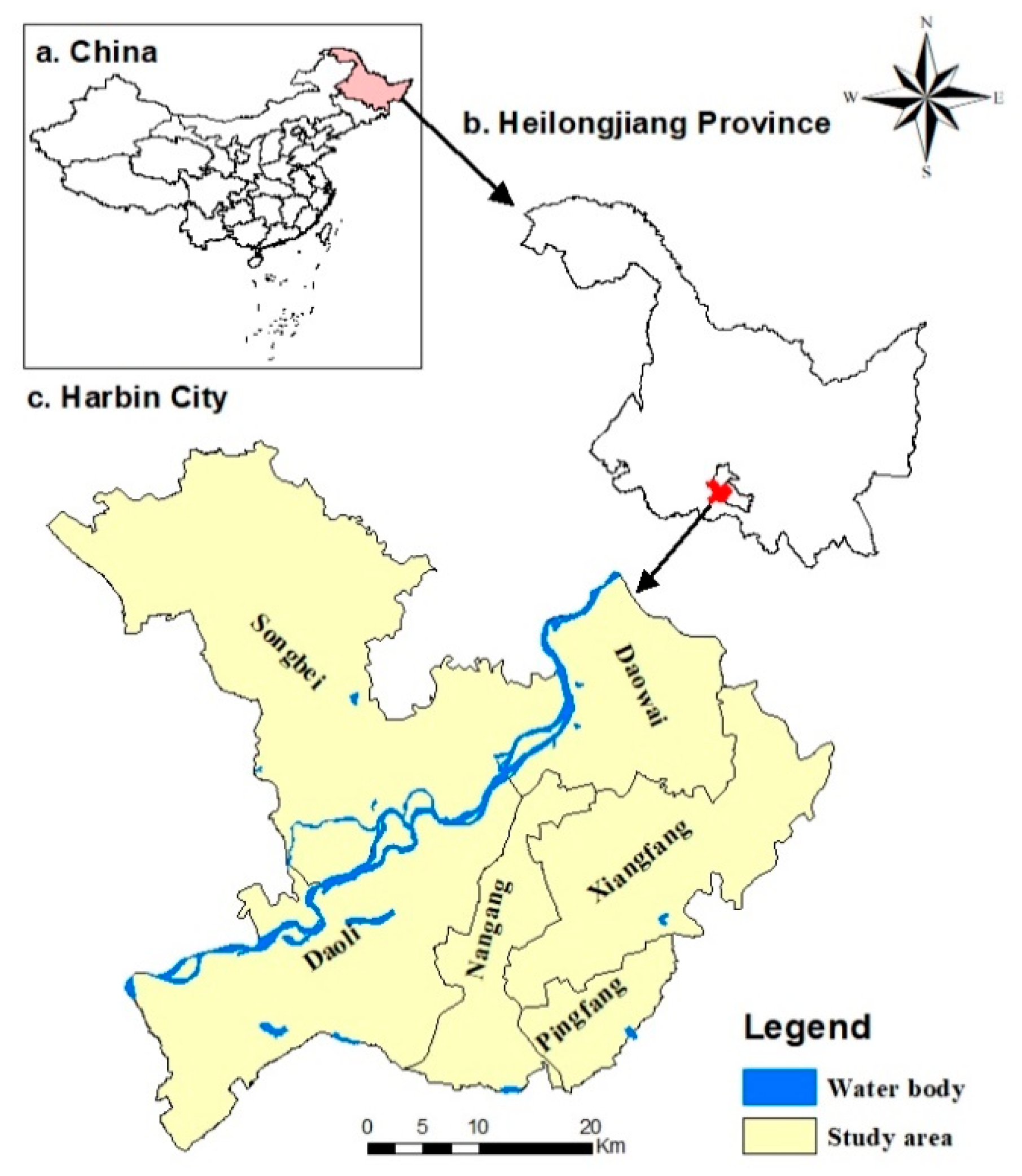
2.1. Study Area
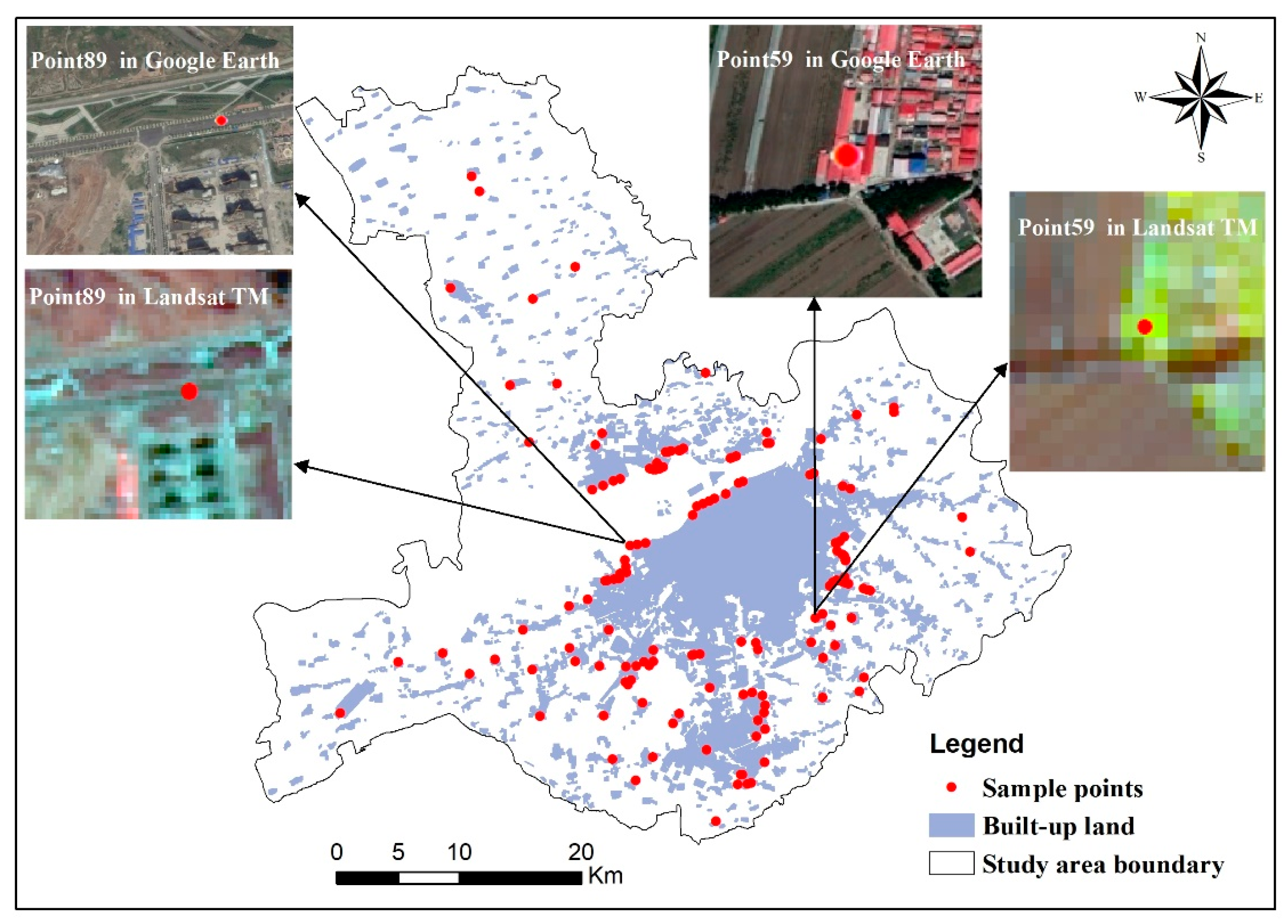
2.2. Data Source
2.3. Methods
2.3.1. The SSM Development Process
2.3.2. Maximum Fragmentation Boundary (MFB) Identification
2.3.3. Detecting Urban Expanding Patterns
3. Results
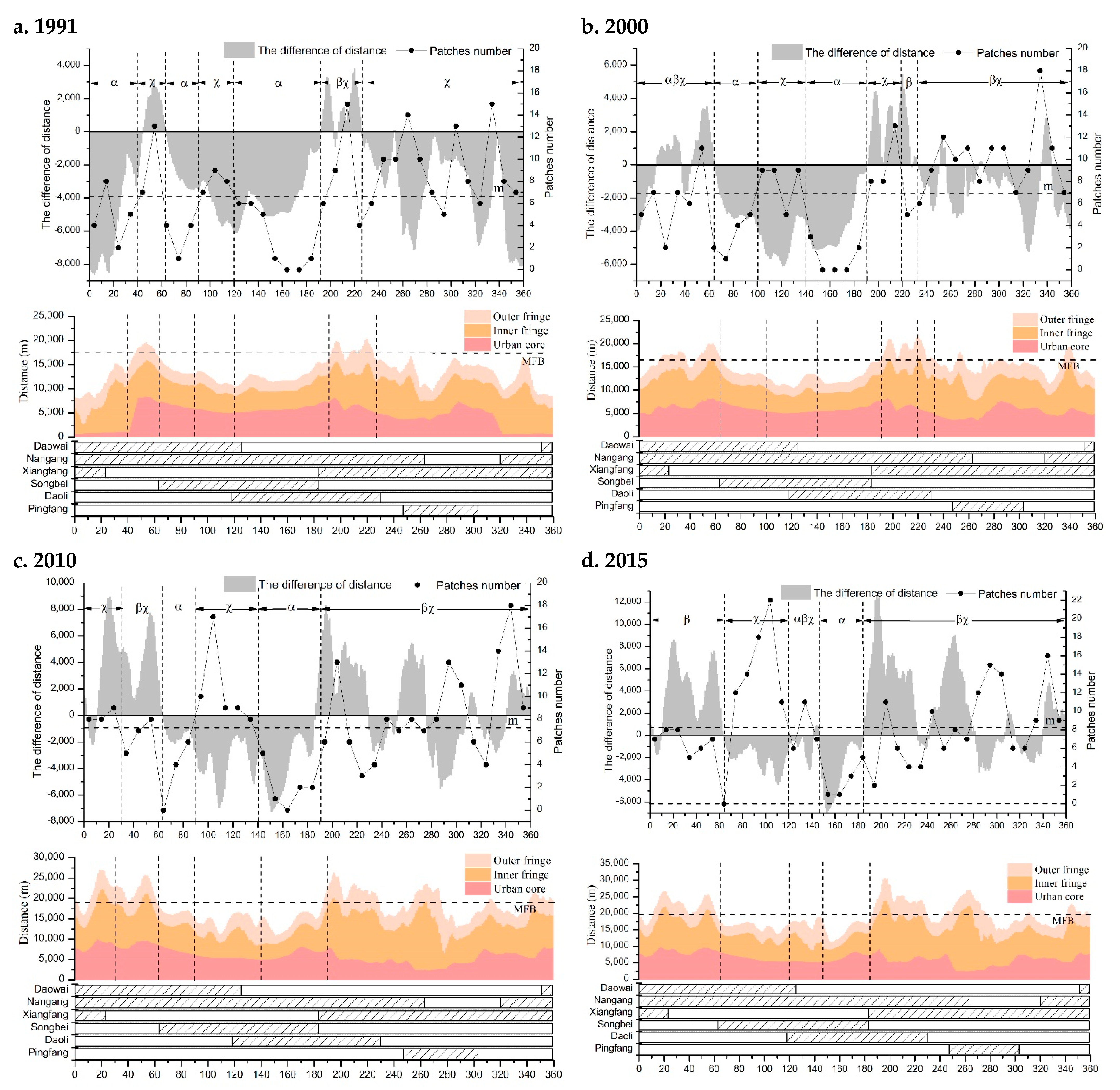
3.1. Changes of the Urban Fringe in Harbin
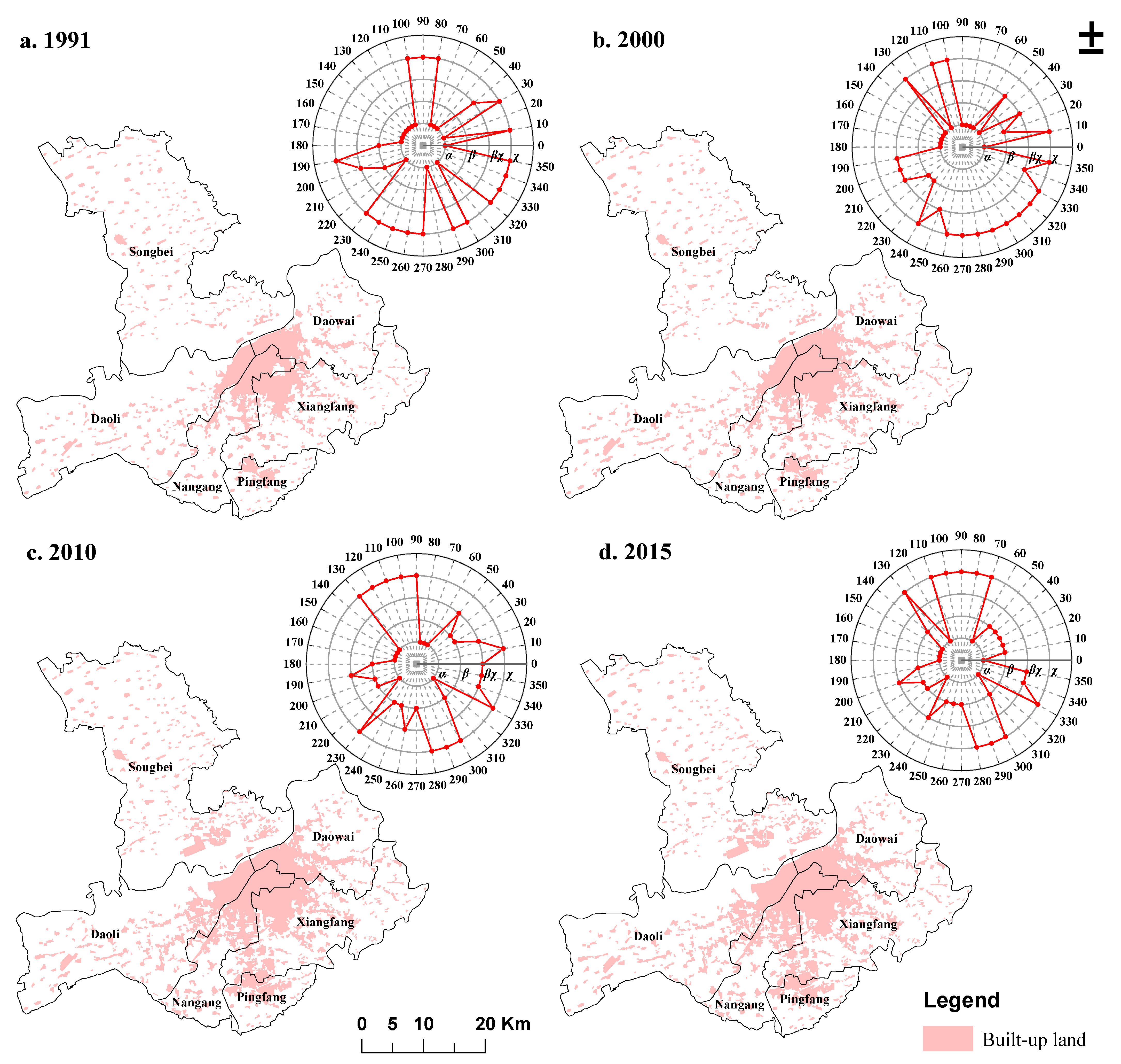
3.2. Changes of Urban Expanding Patterns
4. Discussion
4.1. The Model of Detecting Urban Fringe
4.2. Expanding Trends and Driving Factors in Urban Fringe
5. Conclusions
Supplementary Materials
Author Contributions
Funding
Institutional Review Board Statement
Informed Consent Statement
Data Availability Statement
Acknowledgments
Conflicts of Interest
References
- Vizzari, M.; Sigura, M. Landscape Sequences along the Urban-Rural-Natural Gradient: A Novel Geospatial Approach for Identification and Analysis. Landsc. Urban. Plan. 2015, 140, 42–55. [Google Scholar] [CrossRef]
- Pryor, R.J. Defining the Rural-Urban Fringe. Soc. Forces 1968, 47, 202–215. [Google Scholar] [CrossRef]
- Dadashpoor, H.; Ahani, S. A Conceptual Typology of the Spatial Territories of the Peripheral Areas of Metropolises. Habitat Int. 2019, 90, 102015. [Google Scholar] [CrossRef]
- d’Amour, C.B.; Reitsma, F.; Baiocchi, G.; Barthel, S.; Güneralp, B.; Erb, K.-H.; Haberl, H.; Creutzig, F.; Seto, K.C. Future Urban Land Expansion and Implications for Global Croplands. Proc. Natl. Acad. Sci. USA 2017, 114, 8939. [Google Scholar] [CrossRef] [PubMed] [Green Version]
- Piorr, A.; Ravetz, J.; Tosics, I. Peri-Urbanisation in Europe: Towards European Policies to Sustain Urban-Rural Futures-Synthesis Report; Forest and Landscape, University of Copenhagen: Copenhagen, Denmark, 2011. [Google Scholar]
- Van Vliet, J. Direct and Indirect Loss of Natural Area from Urban Expansion. Nat. Sustain. 2019, 2, 755–763. [Google Scholar] [CrossRef]
- Jiang, Y.; Swallow, S.K. Providing an Ecologically Sound Community Landscape at the Urban-Rural Fringe: A Conceptual, Integrated Model. J. Land Use Sci. 2015, 10, 323–341. [Google Scholar] [CrossRef]
- Pham, V.C.; Pham, T.-T.-H.; Tong, T.H.A.; Nguyen, T.T.H.; Pham, N.H. The Conversion of Agricultural Land in the Peri-Urban Areas of Hanoi (Vietnam): Patterns in Space and Time. J. Land Use Sci. 2015, 10, 224–242. [Google Scholar] [CrossRef]
- Webster, D. An Overdue Agenda: Systematizing East Asian Peri-Urban Research. Pac. Aff. 2011, 84, 631–642. [Google Scholar] [CrossRef]
- Irwin, E.G.; Bockstael, N.E. The Evolution of Urban Sprawl: Evidence of Spatial Heterogeneity and Increasing Land Fragmentation. Proc. Natl. Acad. Sci. USA 2007, 104, 20672. [Google Scholar] [CrossRef] [Green Version]
- Cheng, L.; Xia, N.; Jiang, P.; Zhong, L.; Pian, Y.; Duan, Y.; Huang, Q.; Li, M. Analysis of Farmland Fragmentation in China Modernization Demonstration Zone Since “Reform and Openness”: A Case Study of South Jiangsu Province. Sci. Rep. UK 2015, 5, 11797. [Google Scholar] [CrossRef] [Green Version]
- Fahrig, L. Effects of Habitat Fragmentation on Biodiversity. Annu. Rev. Ecol. Evol. Syst. 2003, 34, 487–515. [Google Scholar] [CrossRef] [Green Version]
- Forman, R.T.T. Land Mosaics: The Ecology of Landscapes and Regions. In The Ecological Design and Planning Reader; Ndubisi, F.O., Ed.; IslandPress: Washington, DC, USA, 2014; pp. 217–234. [Google Scholar]
- Allan, J.D. Landscapes and Riverscapes: The Influence of Land Use on Stream Ecosystems. Annu. Rev. Ecol. Evol. Syst. 2004, 35, 257–284. [Google Scholar] [CrossRef] [Green Version]
- Haase, D.; Nuissl, H. The Urban-to-Rural Gradient of Land Use Change and Impervious Cover: A Long-Term Trajectory for the City of Leipzig. J. Land Use Sci. 2010, 5, 123–141. [Google Scholar] [CrossRef]
- Kuang, W.; Liu, J.; Dong, J.; Chi, W.; Zhang, C. The Rapid and Massive Urban and Industrial Land Expansions in China between 1990 and 2010: A CLUD-Based Analysis of Their Trajectories, Patterns, and Drivers. Landsc. Urban. Plan. 2016, 145, 21–33. [Google Scholar] [CrossRef]
- Lambin, E.F.; Meyfroidt, P. Land Use Transitions: Socio-Ecological Feedback versus Socio-Economic Change. Land Use Policy 2010, 27, 108–118. [Google Scholar] [CrossRef]
- Nagendra, H.; Unnikrishnan, H.; Sen, S. Villages in the City: Spatial and Temporal Heterogeneity in Rurality and Urbanity in Bangalore, India. Land 2014, 3, 1. [Google Scholar] [CrossRef]
- Seto, K.C.; Sánchez-Rodríguez, R.; Fragkias, M. The New Geography of Contemporary Urbanization and the Environment. Annu. Rev. Environ. Resour. 2010, 35, 167–194. [Google Scholar] [CrossRef] [Green Version]
- Wadduwage, S.; Millington, A.; Crossman, N.D.; Sandhu, H. Agricultural Land Fragmentation at Urban Fringes: An Application of Urban-To-Rural Gradient Analysis in Adelaide. Land 2017, 6, 28. [Google Scholar] [CrossRef] [Green Version]
- Liu, Y.; Feng, Y.; Pontius, R.G. Spatially-Explicit Simulation of Urban Growth through Self-Adaptive Genetic Algorithm and Cellular Automata Modelling. Land 2014, 3, 719. [Google Scholar] [CrossRef] [Green Version]
- Rauws, W.S.; de Roo, G. Exploring Transitions in the Peri-Urban Area. Plan. Theory Pract. 2011, 12, 269–284. [Google Scholar] [CrossRef] [Green Version]
- Wang, Y.; van Vliet, J.; Debonne, N.; Pu, L.; Verburg, P.H. Settlement Changes After Peak Population: Land System Projections for China Until 2050. Landsc. Urban. Plan. 2021, 209, 104045. [Google Scholar] [CrossRef]
- Long, H.; Liu, Y.; Wu, X.; Dong, G. Spatio-Temporal Dynamic Patterns of Farmland and Rural Settlements in Su-Xi-Chang Region: Implications for Building a New Countryside in Coastal China. Land Use Policy 2009, 26, 322–333. [Google Scholar] [CrossRef]
- Wang, Y.; van Vliet, J.; Pu, L.; Verburg, P.H. Modeling Different Urban Change Trajectories and Their Trade-Offs with Food Production in Jiangsu Province, China. Comput. Environ. Urban. Syst. 2019, 77, 101355. [Google Scholar] [CrossRef]
- Yang, R.; Zhang, J.; Xu, Q.; Luo, X. Urban-Rural Spatial Transformation Process and Influences from the Perspective of Land Use: A Case Study of the Pearl River Delta Region. Habitat Int. 2020, 104, 102234. [Google Scholar] [CrossRef]
- Andersson, E.; Ahrné, K.; Pyykönen, M.; Elmqvist, T. Patterns and Scale Relations among Urbanization Measures in Stockholm, Sweden. Landsc. Ecol. 2009, 24, 1331–1339. [Google Scholar] [CrossRef] [Green Version]
- Kroll, F.; Müller, F.; Haase, D.; Fohrer, N. Rural-Urban Gradient Analysis of Ecosystem Services Supply and Demand Dynamics. Land Use Policy 2012, 29, 521–535. [Google Scholar] [CrossRef]
- van Vliet, J.; Verburg, P.H.; Grădinaru, S.R.; Hersperger, A.M. Beyond the Urban-Rural Dichotomy: Towards a More Nuanced Analysis of Changes in Built-Up Land. Comput. Environ. Urban. Syst. 2019, 74, 41–49. [Google Scholar] [CrossRef]
- Bridges, L.M.; Crompton, A.E.; Schaefer, J.A. Landscapes as Gradients: The Spatial Structure of Terrestrial Ecosystem Components in Southern Ontario, Canada. Ecol. Complex. 2007, 4, 34–41. [Google Scholar] [CrossRef]
- Luck, M.; Wu, J. A Gradient Analysis of Urban Landscape Pattern: A Case Study from the Phoenix Metropolitan Region, Arizona, USA. Landsc. Ecol. 2002, 17, 327–339. [Google Scholar] [CrossRef]
- Warren, P.S.; Ryan, R.L.; Lerman, S.B.; Tooke, K.A. Social and Institutional Factors Associated with Land Use and Forest Conservation along Two Urban Gradients in Massachusetts. Landsc. Urban. Plan. 2011, 102, 82–92. [Google Scholar] [CrossRef]
- Bryant, C.R.; Russwurm, L.; McLellan, A.G. The City’s Countryside. Land and Its Management in the Rural-Urban Fringe; Longman: London, UK; New York, NY, USA, 1982. [Google Scholar]
- Garreau, J. Edge City: Life on the New Frontier; Anchor: New York, NY, USA, 1992. [Google Scholar]
- Liu, Z.; Robinson, G.M. Residential Development in the Peri-Urban Fringe: The Example of Adelaide, South Australia. Land Use Policy 2016, 57, 179–192. [Google Scholar] [CrossRef]
- Zhang, N.; Fang, L.-N.; Zhou, J.; Song, J.-P.; Jiang, J. The Study on Spatial Expansion and Its Driving Forces in the Urban Fringe of Beijing. Geogr. Res. 2010, 3, 471–480. [Google Scholar]
- Ahani, S.; Dadashpoor, H. A Review of Domains, Approaches, Methods and Indicators in Peri-Urbanization Literature. Habitat Int. 2021, 114, 102387. [Google Scholar] [CrossRef]
- Peng, J.; Zhao, S.; Liu, Y.; Tian, L. Identifying the Urban-Rural Fringe Using Wavelet Transform and Kernel Density Estimation: A Case Study in Beijing City, China. Environ. Model. Softw. 2016, 83, 286–302. [Google Scholar] [CrossRef]
- Wei, W.; Cai, D.; Li, M.; Chen, Z.; Li, F. A method of division of urban fringe based on message entropy: A case study in Nanjing City. In Proceedings of the 2009 Joint Urban Remote Sensing Event, Shanghai, China, 20–22 May 2009; pp. 1–5. [Google Scholar]
- Yao, Y. Spatial Development of Urban Fringe: A Case Study of Haidian District, Beijing. J. Geo. Inf. Sci. 2014, 16, 214–224. [Google Scholar] [CrossRef]
- Chen, X.; Zhang, H.; Liu, Q. Spatial Pattern of Non-Agricultural Land in the Urban Fringe of Beijing. Resour. Sci. 2004, 129–137. [Google Scholar]
- Wu, Z.-Z.; Song, J.-P.; Wang, X.-X.; Cheng, Y.; Zhang, N. On Urbanization Process and Spatial Expansion in the Urban Fringe of Beijing: A Case Study of Daxing District. Geogr. Res. 2008, 27, 285–293, 483. [Google Scholar]
- Feng, L.; Du, P.J.; Li, H.; Zhu, L.J. Measurement of Urban Fringe Sprawl in Nanjing between 1984 and 2010 Using Multidimensional Indicators. Geogr. Res. 2015, 53, 184–198. [Google Scholar] [CrossRef]
- Sui, C.; Lu, W. Study on the Urban Fringe Based on the Expansion-Shrinking Dynamic Pattern. Sustainability 2021, 13, 5718. [Google Scholar] [CrossRef]
- Ma, Y.; Xu, R. Remote Sensing Monitoring and Driving Force Analysis of Urban Expansion in Guangzhou City, China. Habitat Int. 2010, 34, 228–235. [Google Scholar] [CrossRef]
- Wang, X.; Liu, J.; Zhuang, D.; Wang, L. Spatial-Temporal Changes of Urban Spatial Morphology in China. Acta Geogr. Sin. 2005, 60, 392–400. [Google Scholar]
- Yin, J.; Yin, Z.; Zhong, H.; Xu, S.; Hu, X.; Wang, J.; Wu, J. Monitoring Urban Expansion and Land Use/Land Cover Changes of Shanghai Metropolitan Area During the Transitional Economy (1979–2009) in China. Environ. Monit. Assess. 2011, 177, 609–621. [Google Scholar] [CrossRef]
- Gao, J.; Chen, J.; Yuan, F.; Wei Yehua, D.; Chen, W. Patterns, Functions and Underlying Mechanisms of Urban Land Expansion in Nanjing. Geogr. Res. 2015, 33, 1892–1907. [Google Scholar]
- Liu, J.; Wang, X.; Zhuang, D. Application of Convex Hull in Identifying the Types of Urban Land Expansion. Acta Geogr. Sin. Chin. Ed. 2003, 58, 885–892. [Google Scholar]
- National Bureau of Statistics of China. China Statistical Yearbook; China Statistics Press: Beijing, China, 2016.
- Cai, C.; Shang, J. Comprehensive Evaluation on Urban Sustainable Development of Harbin City in Northeast China. Chin. Geogr. Sci. 2009, 19, 144–150. [Google Scholar] [CrossRef]
- Li, W.; Qu, L. Changing Features and Trend of Light Industry Distribution in Northeast China. Chin. Geogr. Sci. 1991, 1, 359–369. [Google Scholar] [CrossRef]
- Yang, D.; Zhao, Z. Investment Explanation of Stagnation of Economic Growth in Northeast China. Northeast. Asia Forum 2015, 2, 94–107. [Google Scholar] [CrossRef]
- Xie, L.; Yang, Z.; Cai, J.; Cheng, Z.; Wen, T.; Song, T. Harbin: A Rust Belt City Revival from Its Strategic Position. Cities 2016, 58, 26–38. [Google Scholar] [CrossRef]
- Xi, F.; He, H.S.; Clarke, K.C.; Hu, Y.; Wu, X.; Liu, M.; Shi, T.; Geng, Y.; Gao, C. The Potential Impacts of Sprawl on Farmland in Northeast China-Evaluating a New Strategy for Rural Development. Landsc. Urban Plan. 2012, 104, 34–46. [Google Scholar] [CrossRef]
- Christaller, W. Die Zentralen Orte in Süddeutschland: Eine Ökonomisch-Geographische Untersuchung über die Gesetzmässigkeit der Verbreitung und Entwicklung der Siedlungen mit Städtischen Funktionen; Wissenschaftliche BuchgesellSchaft: Darmstadt, Germany, 1980. [Google Scholar]
- Weber, A. On the Location of Industries. Prog. Hum. Geogr. 1982, 6, 120–128. [Google Scholar] [CrossRef]
- Getis, A.; Fellmann, J.D.; Getis, J.; Barker, B.W. Introduction to Geography; William C. Brown Publishers: Dubuque, IA, USA, 1994. [Google Scholar]
- Liang, J. Fourteen Principles in Geography. Sci. Geogr. Sin. 2009, 29, 307–315. [Google Scholar]
- Davidson, C. Issues in Measuring Landscape Fragmentation. Wildl. Soc. Bull. 1998, 26, 32–37. [Google Scholar]
- Bogaert, J.; Van Hecke, P.; Eysenrode, D.S.-V.; Impens, I. Landscape Fragmentation Assessment Using a Single Measure. Wildl. Soc. Bull. 2000, 28, 875–881. [Google Scholar]
- Nagendra, H.; Munroe, D.K.; Southworth, J. From Pattern to Process: Landscape Fragmentation and the Analysis of Land Use/Land Cover Change. Agric. Ecosyst. Environ. 2004, 101, 111–115. [Google Scholar] [CrossRef]
- Von Thünen, J. Der Isolirte Staat (The Isolated State); Wiegandt, Hempel & Parey: Berlin, Germany, 1875. [Google Scholar]
- Sun, Y.; Zhao, S.; Qu, W. Quantifying Spatiotemporal Patterns of Urban Expansion in Three Capital Cities in Northeast China Over the Past Three Decades Using Satellite Data Sets. Environ. Earth Sci. 2015, 73, 7221–7235. [Google Scholar] [CrossRef]
- Gao, J.; Wei, Y.D.; Chen, W.; Yenneti, K. Urban Land Expansion and Structural Change in the Yangtze River Delta, China. Sustainability 2015, 7, 281. [Google Scholar] [CrossRef] [Green Version]
- Tian, G.; Jiang, J.; Yang, Z.; Zhang, Y. The Urban Growth, Size Distribution and Spatio-Temporal Dynamic Pattern of the Yangtze River Delta Megalopolitan Region, China. Ecol. Model. 2011, 222, 865–878. [Google Scholar] [CrossRef]
- Xiao, J.; Shen, Y.; Ge, J.; Tateishi, R.; Tang, C.; Liang, Y.; Huang, Z. Evaluating Urban Expansion and Land Use Change in Shijiazhuang, China, by Using GIS and Remote Sensing. Landsc. Urban Plan. 2006, 75, 69–80. [Google Scholar] [CrossRef]
- Arsanjani, J.J.; Helbich, M.; Mousivand, A.J. A Morphological Approach to Predicting Urban Expansion. Trans. GIS 2014, 18, 219–233. [Google Scholar] [CrossRef]
- Mattikalli, N.M. Integration of Remotely-Sensed Raster Data with a Vector-Based Geographical Information System for Land-Use Change Detection. Int. J. Remote. Sens. 1995, 16, 2813–2828. [Google Scholar] [CrossRef]
- Lu, D.; Song, K.; Zeng, L.; Liu, D.; Khan, S.; Zhang, B.; Wang, Z.; Jin, C. Estimating Impervious Surface for the Urban Area Expansion: Examples From Changchun, Northeast China. Int. Arch. Photogramm. Remote. Sens. Spat. Inf. Sci. 2008, 36, 385–391. [Google Scholar]
- Kim, S.; Jang, N. Seoul and the World’s Metropolis: A Comparison of Urban Changes after the Millennium; Seoul Research Institute: Seoul, Korea, 2017. [Google Scholar]
- Mahtta, R.; Mahendra, A.; Seto, K.C. Building Up or Spreading Out? Typologies of Urban Growth across 478 Cities of 1 Million +. Environ. Res. Lett. 2019, 14, 124077. [Google Scholar] [CrossRef] [Green Version]
- World Bank. East Asia’s Changing Urban Landscape: Measuring a Decade of Spatial Growth; World Bank: Washington, DC, USA, 2015. [Google Scholar]
- Glaeser, E.; Huang, W.; Ma, Y.; Shleifer, A. A Real Estate Boom with Chinese Characteristics. J. Econ. Perspect. 2017, 31, 93–116. [Google Scholar] [CrossRef] [Green Version]
- Dubeaux, S.; Cunningham-Sabot, E. Maximizing the Potential of Vacant Spaces within Shrinking Cities, a German Approach. Cities 2018, 75, 6–11. [Google Scholar] [CrossRef]
- Xie, Y.; Gong, H.; Lan, H.; Zeng, S. Examining Shrinking City of Detroit in the Context of Socio-Spatial Inequalities. Landsc. Urban. Plan. 2018, 177, 350–361. [Google Scholar] [CrossRef]
- Xia, C.; Zhang, A.; Wang, H.; Yeh, A.G.O. Predicting the Expansion of Urban Boundary Using Space Syntax and Multivariate Regression Model. Habitat Int. 2019, 86, 126–134. [Google Scholar] [CrossRef]
- Long, H. Land Use Policy in China: Introduction. Land Use Policy 2014, 40, 1–5. [Google Scholar] [CrossRef]


| Year | Entity ID | Acquisition Date | Data Set | Spatial Resolution |
|---|---|---|---|---|
| 1991 | LT51180281991165HAJ00 | 1991-06-14 | Landsat 4-5 TM | 30 m |
| 2000 | LT51180282000158HAJ03 | 2000-06-06 | Landsat 4-5 TM | 30 m |
| 2010 | LT51180282010265MGR01 | 2010-09-22 | Landsat 4-5 TM | 30 m |
| 2015 | LC81180282015167LGN00 | 2015-06-16 | Landsat 8 OLI/TIRS | 15 m |
| Urban Core | Urban Fringe | |||||||
|---|---|---|---|---|---|---|---|---|
| 1991 | 2000 | 2010 | 2015 | 1991 | 2000 | 2010 | 2015 | |
| Railway | 0.18 | 0.17 | 0.16 | 0.15 | 0.09 | 0.08 | 0.07 | 0.06 |
| Expressway | 0.00 | 0.00 | 0.00 | 0.00 | 0.71 | 0.77 | 0.64 | 0.66 |
| State Road | 0.59 | 0.44 | 0.39 | 0.46 | 0.49 | 0.52 | 0.42 | 0.39 |
| City Roads | 32.26 | 30.66 | 29.09 | 28.12 | 7.79 | 6.11 | 4.99 | 4.55 |
| First-class | 11.28 | 10.83 | 10.62 | 10.54 | 2.71 | 2.07 | 1.62 | 1.38 |
| Second-class | 20.98 | 19.83 | 18.46 | 17.58 | 5.08 | 4.03 | 3.37 | 3.17 |
Publisher’s Note: MDPI stays neutral with regard to jurisdictional claims in published maps and institutional affiliations. |
© 2021 by the authors. Licensee MDPI, Basel, Switzerland. This article is an open access article distributed under the terms and conditions of the Creative Commons Attribution (CC BY) license (https://creativecommons.org/licenses/by/4.0/).
Share and Cite
Wang, Y.; Han, Y.; Pu, L.; Jiang, B.; Yuan, S.; Xu, Y. A Novel Model for Detecting Urban Fringe and Its Expanding Patterns: An Application in Harbin City, China. Land 2021, 10, 876. https://doi.org/10.3390/land10080876
Wang Y, Han Y, Pu L, Jiang B, Yuan S, Xu Y. A Novel Model for Detecting Urban Fringe and Its Expanding Patterns: An Application in Harbin City, China. Land. 2021; 10(8):876. https://doi.org/10.3390/land10080876
Chicago/Turabian StyleWang, Yuan, Yilong Han, Lijie Pu, Bo Jiang, Shaofeng Yuan, and Yan Xu. 2021. "A Novel Model for Detecting Urban Fringe and Its Expanding Patterns: An Application in Harbin City, China" Land 10, no. 8: 876. https://doi.org/10.3390/land10080876
APA StyleWang, Y., Han, Y., Pu, L., Jiang, B., Yuan, S., & Xu, Y. (2021). A Novel Model for Detecting Urban Fringe and Its Expanding Patterns: An Application in Harbin City, China. Land, 10(8), 876. https://doi.org/10.3390/land10080876