Multi-Year Mapping of Disturbance and Reclamation Patterns over Tronox’s Hillendale Mine, South Africa with DBEST and Google Earth Engine

Abstract

This study was devised to examine the pattern of disturbance and reclamation by Tronox, which instigated a closure process for its Hillendale mine site in South Africa, where they recovered zirconium- and titanium-bearing minerals from 2001 to 2013. Restoring mined-out areas is of great importance in South Africa, with its ominous record of almost 6000 abandoned mines since the 1860s. In 2002, the government enacted the Mineral and Petroleum Resources Development Act (No. 28 of 2002) to enforce extracting companies to restore mined-out areas before pursuing closure permits. Thus, the trajectory of the Hillendale mine remains unstudied despite advances in the satellite remote sensing technology that is widely used in this field. Here, we retrieved a collection of Landsat-derived normalized difference vegetation index (NDVI) within the Google Earth Engine and applied the Detecting Breakpoints and Estimating Segments in Trend (DBEST) algorithm to examine the progress of vegetation transformation over the Hillendale mine between 2001 and 2019. Our results showed key breakpoints in NDVI, a drop from 2001, reaching the lowest point in 2009–2011, with a marked recovery pattern after 2013 when the restoration program started. We also validated our results using a random forests strategy that separated vegetated and non-vegetated areas with an accuracy exceeding 78%. Overall, our findings are expected to encourage users to replicate this affordable application, particularly in emerging countries with similar cases.

1. Introduction

South Africa is richly endowed with a variety of mineral resources and is among the most prominent raw material exporters in the world. In recent years, the demand for zirconium-bearing minerals, of which South Africa holds most of the world’s reserves, has proliferated [1]. This has had important socio-economic implications for South Africa as the second-largest producer of this commodity (19.4%) after Australia (41.7%), together accounting for 44 Mt (61%) of the 72 Mt world total reserve base [2]. Typically, zirconium is found in association with the principal titanium minerals ilmenite and rutile, thus providing more commercial sources for zircon [3]. The extraction of these heavy sand minerals is a mature enterprise in South Africa with three currently active production mines: Richards Bay Minerals (RBM) and Tronox, both in KwaZulu-Natal (KZN) and Namakwa Sands in the Western Cape province [4]. Our focus here is mainly on the northeast coast of KwaZulu-Natal province, where Tronox KZN Sands recover these deposits by completely obliterating the existing vegetation. Within this mineral-rich coastal area, its operation consists of the currently active Fairbreeze mine and the other in the closure stage at Hillendale, which is the subject of this paper [5].

The realization of sustainable mining has become a global priority, mainly because mine closure is increasingly accepted to restore the land to a workable post-mining state, such as for agriculture [6] and tourism [7]. In the context of the sectors mentioned above, a coal-based company, PT Berau Coal in Indonesia, successfully planted cacao trees in its mined-out site after shade trees (F. moluccana) were grown to provide shade for the cacao trees [8], and a former limestone quarry, now Butchart Gardens in Canada, has become the most renowned garden in North America, attracting over one million visitors annually [9]. This is especially pertinent for countries such as South Africa, which has an ominous record of almost 6000 abandoned mines since their inception in the 1860s [10]. Abandoned mines are typically a consequence of elusive mining closure protocols and pose a severe threat to human health, ecological stability, and agricultural practices [11]. Threats such as pollution, ecological degradation, and biodiversity loss have been reported in several mining areas worldwide [12,13,14], defying sustainable development objectives [15]. To alleviate such impacts, the application of mining restoration strategies is necessary [16]. However, the implementation of these plans is generally not enough for extractive mines, mainly because they require continuous monitoring over time [17,18]. More recently, the South African government passed the Mineral and Petroleum Resources Development Act (MPRDA) (No. 28 of 2002), making it compulsory for mining companies to rehabilitate after operations had ceased [19]. As a result of this Act, all mining companies are required to set aside financial provisions for the discharge of their rehabilitation obligations, which can be reimbursed on the issuance of a closure certificate by the state regulator [20]. However, the issuance of a closure certificate implies that the state incurs financial liability to rehabilitate the land [21], and the government is currently facing an estimated cost of ZAR 30 billion (USD 2 billion) for this task [20].

The monitoring of the mine rehabilitation process necessitates suitable indicators [22] to facilitate the understanding and interpretation of the outcome by various stakeholders, such as the company, environmental agencies, and the immediate communities concerned with the recovery [16]. The standard indicator used to evaluate the restoration progress of mining areas is related to vegetation [18,23] due to its strong impact on soil erosion and the physicochemical properties of the soil [24]. The evaluation of vegetation disturbance and recovery progression in mining environments is a challenging exercise [25,26], and to warrant legislative compliance, continuous monitoring of mine rehabilitation is crucial [18]. Remote sensing has become the most practical and objective means to address this task. It provides complete coverage of the mining area and enables repetitive observation with products such as Landsat available for free [27]. Landsat imagery has the suitable spatial and spectral attributes to meet the various vegetation mapping requirements using different vegetation indices [28,29]. The normalized difference vegetation index (NDVI; [30]) is the most widespread vegetation indicator computed from visible and near-infrared (NIR) bands and is highly sensitive to modifications in vegetation growth, hence its extensive use in mine reclamation efforts [18].

Rapid advances in the spectral time-series approach that exploits the complete record of usable imagery provide the means of capturing landscape dynamics over their entire duration, whether short or long term [31]. The Landsat-based Detection of Trends in Disturbance and Recovery (LandTrendr; [32]) and the Breaks for Additive Season and Trend (BFAST; [33]) are, so far, the most widely applied methods for this purpose. However, Wang et al. [34] found these methods to be restricted by factors such as satellite sensors, data types, and lengths and concluded that their versatility needs to be enhanced. Alternatively, Jamali et al. [35] developed Detecting Breakpoints and Estimating Segments in Trend (DBEST), which overcome these limitations and can handle periodic and non-periodic remotely sensed time-series data with better versatility. Hitherto, few studies have tested the performance of DBEST. The earlier approaches have also been embedded and implemented in the Google Earth Engine (GEE) cloud-based computing asset, which host the entire Landsat archive as well as several processing functions (more details in Section 2.5).

A growing number of studies have validated the capacity of the GEE resources by detecting and tracking the evolution of mining-induced landscape dynamics with a high degree of success. For example, Dlamini and Xulu [36] used the GEE-based LandTrendr algorithm to document the effective RBM restoration in South Africa from 1984 to 2018. They also applied a random forests (RF) classifier to distinguish vegetation from non-vegetated with an overall accuracy exceeding 90%. In a similar study, Xiao et al. [37] mapped mining-induced disturbance and reclamation in Shengli Coalfield in China using LandTrendr and GEE, and their results showed a 26% reclamation rate. Furthermore, Ang et al. [38] successfully applied an RF supervised classification to detect a land cover change in mining areas in the Philippines within the GEE environment and achieved high classification accuracy. They also derived socio-economic indicators from land use and cover trends. More recently, He et al. [39] employed Landsat imagery and GEE to monitor the subsidence of water in mining landscapes on the eastern plain in China. They successfully identified subsidence and restoration with accuracies from 79% to 88% using an RF classifier. Despite these advances, several mining areas across the world, and in South Africa in particular, remain unstudied and inconclusive.

In this study, we present a case study demonstrating the restoration of the highly transformed Hillendale mine on the northeast coast of South Africa. At present, this site is in the rehabilitation phase intending to secure a mine closure permit [5], and no study has yet been conducted to examine its trajectory. Thus, our goal is to monitor the progress of this task using GEE and the DBEST algorithm based on Landsat-derived NDVI from 2001 to 2019. To the best of our knowledge, no attempt has yet been made to segment a time series of vegetation index over mining areas using DBEST, and our study is the first trial in this regard. Overall, our results are expected to encourage users to replicate this affordable application, especially in developing countries where similar cases are expected.

2. Materials and Methods

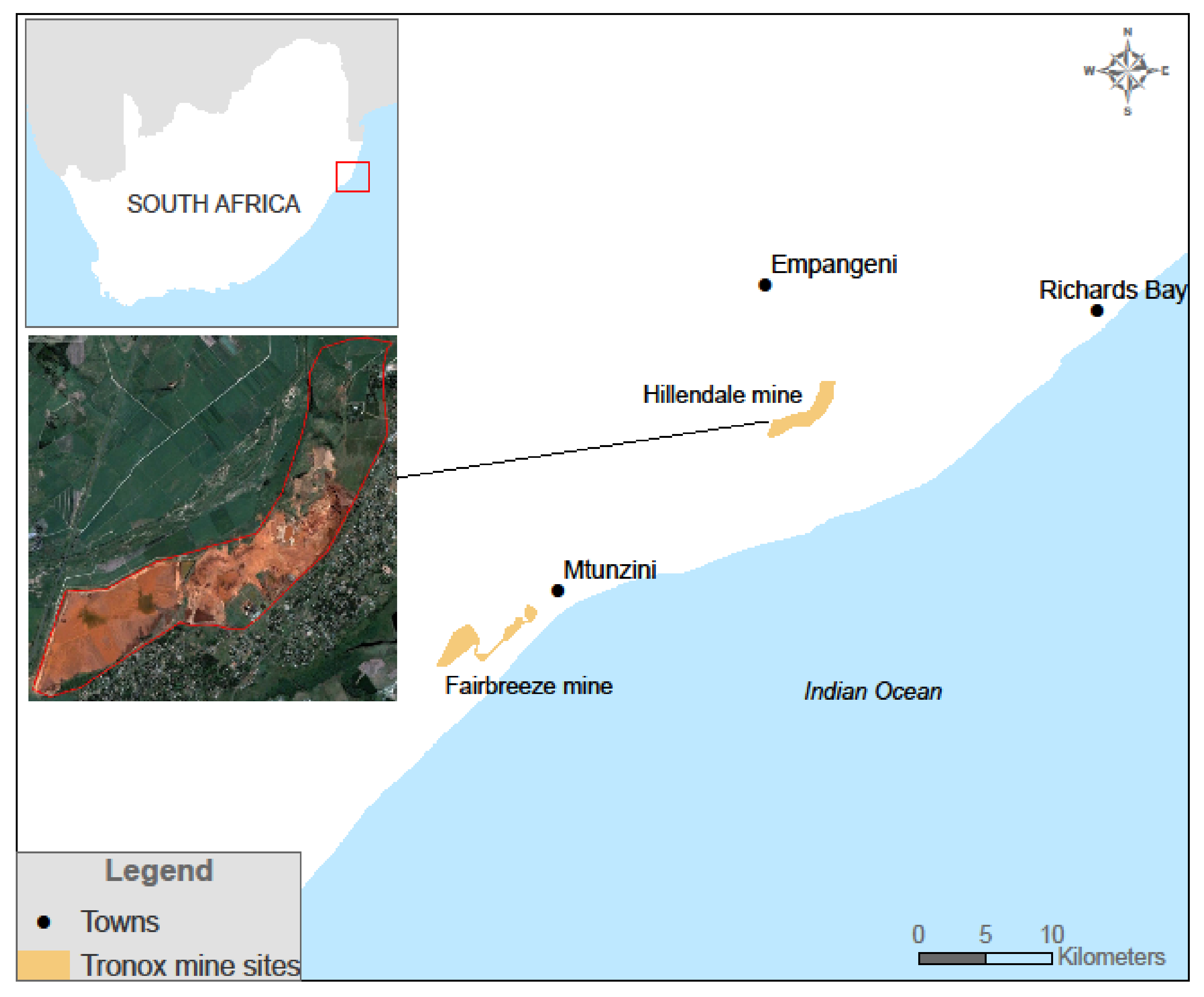
2.1. Site Description

This study was carried out at the Hillendale mine operated by Tronox KZN Sands on the mineral-rich northeast coast of KwaZulu-Natal, near the towns of Empangeni and Richards Bay, South Africa (Figure 1). The site covers 495 ha that was subjected to extensive transformation during its operation between 2001 and 2013. The procedure entailed hydraulic excavation to recover the zirconium- and titanium-bearing heavy minerals from sand dunes. This followed a gravity separation trail to produce a heavy mineral concentrate, with sand tailings reverted to recreate dunes and the bulk of the fines fraction discharged in a residue storage facility (RSF) [5].

Typically, this process completely destroys the soil and associated mineral nutrient balance for plant growth [40]. Before mining, sugarcane plantation was the dominant activity at the Hillendale site [40]. The company is dedicated to rehabilitating the site towards a self-sustaining ecosystem that is intended for sugarcane production again. This area is characterized as subtropical to tropical with hot and humid summers and warm winters, and the mean annual temperature is 21.8 °C. The area is classified as a high rainfall region by South African standards, with a mean yearly rainfall of approximately 1300 mm.

The vegetation used in the rehabilitation varies across the mining area. For instance, the walls of the RSF are planted with kikuyu grass and some indigenous grass species to mitigate erosion problems and enhance the aesthetic of this landscape [41]. The Eucalyptus and Casuarina species are intended for use in the rehabilitation of the RSF through a combination of soil improvement and soil drying [41]. Moreover, while the post-mining land use is aimed at sugar cane, these tree species are currently used for stabilizing the area.

2.2. Satellite Data

We obtained freely available collections of Landsat scenes from the Google Earth Engine (GEE) cloud computing platform using the JavaScript code editor (https://earthengine.google.com/ Mountain View, CA, USA; accessed 25 February 2021). These 30-m Landsat 5, 7, and 8 images were filtered and cloud masked using the JavaScript code editor. Moreover, the images were already orthorectified, and Level 1 Precision Terrain (L1TP) corrected. The L1TP-corrected product fulfills both radiometric and geometric criteria set by USGS (U.S. Geological Survey), and is considered to be of high quality and usable [42]. Following Karan et al.’s [18] study, which found the normalized difference vegetation index (NDVI) to be the best indicator for detecting mine-induced vegetation changes, we computed monthly mean composites of this index from the collection of usable images from 2001 to 2019. The NDVI values were averaged for the entire mining area to get an overall picture of the mine disturbance and recovery patterns. The NDVI is computed by differencing the NIR and red band and dividing by their sum, which is expressed as follows:

$$NDVI=\frac{NIR-Red}{NIR+Red }$$

(1)

where values range between –1 and 1; the negative values reflect an absence of vegetation, while positive values represent vegetative areas. In our context, rehabilitated sites are associated with larger NDVI pixel values than earlier, while lower values indicate exposed soil and very low vegetation cover. However, the resultant time series was irregular because some months had missing observations due to cloud cover. Only the best available cloudless scenes were intended to be used for analysis, as cloud cover is persistent in the studied region. To resolve this problem, we emulated Halabisky et al. [43] and applied spline interpolation to fit a cubic spline to each missing NDVI value over the time series using the R statistical package “spline”. We then denoised the NDVI time series using wavelets to implement our intended algorithm effectively. The denoising procedure is expected to remove the noisy data and retain as much high-quality data as possible [44]. The flowchart is illustrated in Figure 2.

Before the implementation of the change algorithm, it is important to note that NDVI values were averaged for the entire Hillendale mine site, and the mean annual NDVI was used for analysis. This is because rehabilitation efforts in many mining companies are not often implemented across the entire mining area at the same time. Therefore, the averaging of the NDVI for the entire mining area is aimed at considering the overall recovery. We also analyzed patterns of disturbance and recovery in selected mining sites to demonstrate how different sections of the mines are recovering.

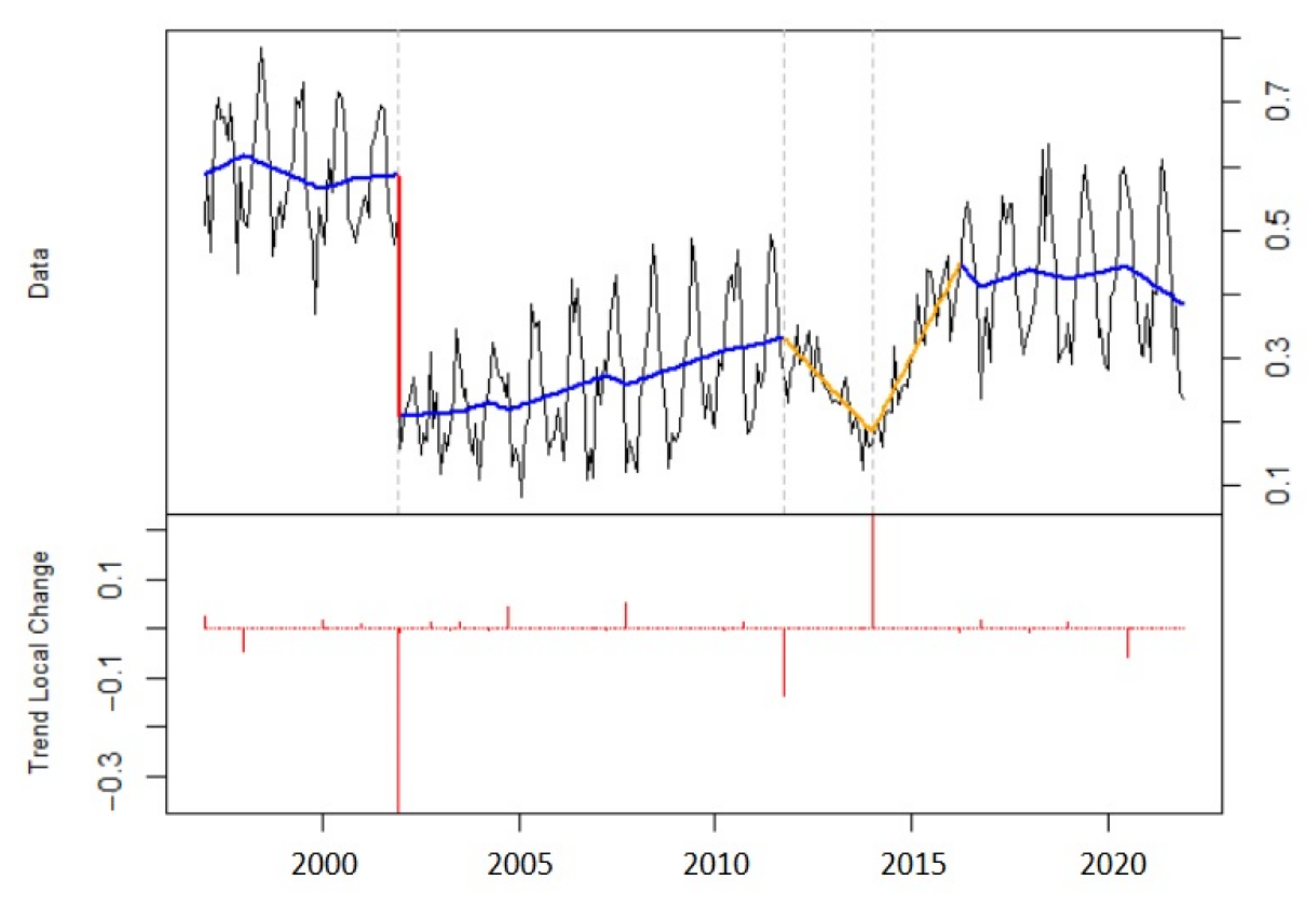
2.3. Change Detection Using DBEST Algorithm

In this study, we applied the Detecting Breakpoints and Estimating Segments in Trend (DBEST; [35]) program for segmenting and analyzing trend changes in the time series of vegetation indices. DBEST has two primary algorithms: the change detection algorithm and the generalization algorithm [35]. The main aim of the change detection algorithm is to detect a trend, determine the type of changes (abrupt or gradual), and estimate change timing, change magnitude, change number, and the direction of change (Figure 3). On the other hand, the generalization algorithm simplifies the detected trend into the main features of the time series. In its operation, DBEST employs a novel segmentation algorithm that estimates the direction into linear segments using one of the three user-defined parameters, namely a generalization-threshold parameter δ, the $m$ most considerable changes, or the threshold $\beta$ for the magnitude of changes of interest for detection [35]. The cited work found DBEST to be a quick, accurate, and flexible tool that determines trend alteration estimating the timing, extent, and direction. This study used the DBEST trend generalization and change detection algorithm to detect breakpoints with the most remarkable changes in NDVI as a proxy for mining-induced disturbance and recovery. We executed the DBEST application in the R environment using the “DBEST’” package [45] (https://cran.r-project.org/web/packages/DBEST/index.html; accessed 1 March 2021).

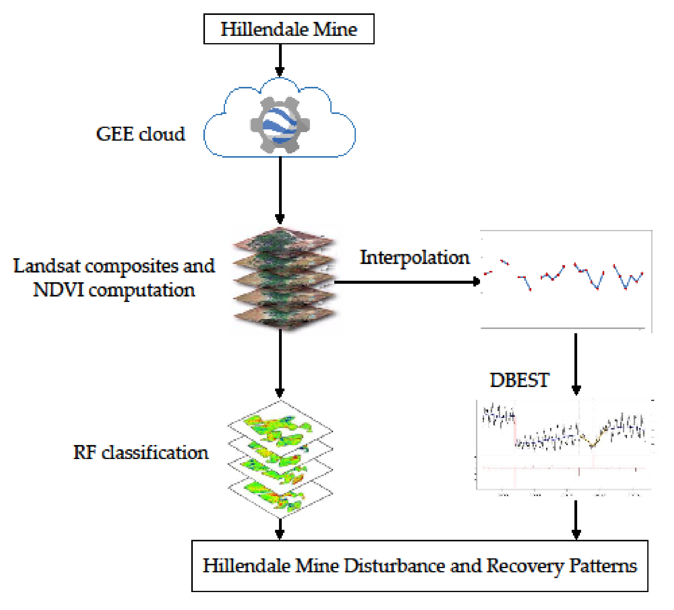
2.4. GEE Framework for Change Monitoring Over Mining Areas

The advent of the Google Earth Engine (GEE) cloud-based platform brought unprecedented transitions in remote sensing and greatly enhanced the democratization of satellite data. The GEE leverages computational services for planetary-scale analysis and consists of petabytes of geospatial data, including a complete archive of Landsat images, climate data, and state-of-the-art algorithms with highly dense time series analysis [46]. Furthermore, the GEE eliminates many resource-based barriers to satellite data gathering, storage, and processing and hosts ready-to-use products such as NDVI [47], permitting users to devote more time to making sense of the data than on preparation. GEE further enables users to share scripts and assets [48]. These attributes have leveled the playing field for all users irrespective of their location, increasingly making GEE the preferred choice for geospatial data analysis [49]. Since its inception, several studies have widely employed GEE in various land use and land cover change applications [49], but relatively few have exploited this asset for monitoring dynamics over mining landscapes, namely only Dlamini and Xulu [36] in South Africa until now.

2.5. Validation and Accuracy Assessment

The study area was categorized into vegetation and non-vegetated classes to analyze the vegetation changes due to mining activity. For validation purposes, we used high-resolution Google Earth Pro to identify reference classes for each pixel sample within the Hillendale site, where 100 samples for each category were determined. Google Earth Pro was the preferred data source to ensure the reliability of the training sample due to limited access and data procurement [50]. We randomly selected samples for each year at fixed locations that were adequately spread over the entire mining site to ensure the diversity of samples for each class, as illustrated in Figure 4.

We then applied a random forests (RF; [51]) algorithm to classify vegetated and non-vegetated classes, and after that, we validated the performance of our classification within the GEE asset (https://developers.google.com/earth-engine/classifcation; accessed 28 February 2021). This process entails the degree to which a classifier correctly separates a random set of samples [52]. RF is a popular machine learning algorithm of object identification and classification within GEE [48] because of its flexibility, non-parametric nature, and ability to limit overfitting [53], and it has displayed superior performance against other classifiers across a variety of datasets [54]. For the classification, the samples were randomly split into 70% for training and 30% for validating the datasets. From the resultant matrix, we calculated a set of accuracy assessment metrics (Equations (2)–(4)). The producer accuracy (PA) is calculated as the number of vegetated pixels that were correctly classified as vegetation, B is the proportion of the mine that was incorrectly classified, user accuracy (UA) is the number of non-vegetated pixels that were incorrectly classified as vegetated, and D is the proportion of non-vegetated pixels that were classified correctly. The overall accuracy (OA) is computed by dividing the correct pixels by the total number of pixels [55]. We also computed the regions of classified areas for each year within the GEE environment.

$$PA=\frac{A}{A+B}$$

(2)

$$UA=\frac{C}{C+D}$$

(3)

$$OA=\frac{A+D}{A+B+C+D}$$

(4)

2.6. Mann–Kendall Test

It is vital to work out the monotonic trends in the time series of any geophysical data. Here, we used the Mann–Kendall (MK) test [56,57,58] to detect the trends in the vegetation and non-vegetated time series extracted in the study area over the study period. The MK test is a non-parametric, rank-based method that is commonly used to extract monotonic trends in the time series of climate data, environmental data, and hydrological data. In this study, the MK test was used for the trend analysis of annual data series for vegetation and non-vegetated area means (in Ha). MK test statistics S can be computed using the formula:

$$S={\displaystyle \sum }_{k=1}^{n-1} {\displaystyle \sum }_{j=k+1}^{n}sgn\left(X_j-X_k\right)$$

(5)

$$sgn\left(x\right)=\left\{\begin{array}{c}+1, \mathrm{if} x>1\\ 0, \mathrm{if} x=0\\ -1, \mathrm{if} x<1\end{array}\right.$$

(6)

where the average value of S is E[S] = 0, and the variance σ^2 was calculated using the following equation:

$${\sigma }^2=\left\{n\left(n-1\right)\left(2n+5\right)-{\displaystyle \sum }_{j=1}^p{t}_j\left(t_j-1\right)\left(2t_j+5\right)\right\}/18$$

(7)

where, $t_j$ is the number of data points in the $j\mathrm{th}$ tied group, and $p$ is the number of the tied group in the time series. Under the assumption of a random and independent time series, the statistical function $S$ is approximately normal distributed given that the following Z-transformation equation is used:

$$Z=\left\{\begin{array}{c}\frac{S-1}{\sigma } \mathrm{if} S>1\\ 0 \mathrm{if} S=0\\ \frac{S+1}{\sigma } \mathrm{if} S<1\end{array}\right.$$

(8)

The value of the statistic $S$ is associated with Kendall’s $\tau =\raisebox{1ex}{$S$}\!\left/ \!\raisebox{-1ex}{$D$}\right.$ where:

$$D={\left[\frac{1}{2}n\left(n-1\right)-\frac{1}{2}{\displaystyle \sum }_{j=1}^p{t}_j\left(t_j-1\right)\right]}^{1/2}{\left[\frac{1}{2}n\left(n-1\right)\right]}^{1/2}$$

(9)

With respect to the above-defined Z-transformation equation, in this study, there is a 5% confidence level, where the null hypothesis of no trend is rejected if $\left|Z\right|$ > 1.96. One other important output of the Mann–Kendall statistic is the Kendall tau $\tau$, which is a measure of a correlation that measures the strength of the relationship between any two independent variables.

Furthermore, the Mann–Kendall trend method can be modified to a sequential version of the Mann–Kendall test statistic, which is called the Sequential Mann–Kendall (SQ-MK). The SQ-MK trend test method was proposed by Sneyers [59], and it can be employed to detect approximate potential trend turning points in long-term time series, as well as the dynamics of the trend along with the time frame. The SQ-MK test method produces a forward/progressive trend ($u\left(t\right)$) and a backward/retrograde trend ($u^{\prime }\left(t\right)$) of the time series. In a mathematical form, SQ-MK is calculated by using ranked values of $y_i$ of a given time series ($x_1, x_2,x_3,\dots ,x_n$). The magnitudes of $y_i, (i=1,2,3,\dots ,$n) are compared with $y_i, (j=1,2,3,\dots ,$ j−1). At each comparison, the number of cases where $y_i>y_j$ are counted and then donated to $n_i$. For effective use of this method, these time series (forward and backward trend) are plotted in the same figure. In the regions where they cross each other and diverge beyond the specific threshold (±1.96 in this study), it is regarded as a statistically significant trend. In addition, the region where they cross each other indicates the time locations where the trend turning point starts [60]. The statistic $t_i$ is is calculated using the following equation:

$$t_i={\displaystyle \sum }_{j=1}^i{n}_i$$

(10)

The mean and variance of the statistic $t_i$ are given by:

$$E\left(t_i\right)=\frac{i\left(i-1\right)}{4}$$

(11)

and:

$$\mathrm{Var}\left(t_i\right)=\frac{i\left(i-1\right)\left(2i-5\right)}{72}$$

(12)

The values of the statistic $u(t_i)$, which are standardized, are calculated using the following equation:

$$u\left(t_i\right)=\frac{t_i-E\left(t_i\right)}{\sqrt{\mathrm{Var}\left(t_i\right)}}$$

(13)

The above equation describes the forward sequential statistic which is also called the progressive statistic. The backward/retrograde statistic values ($u^{\prime }\left(t_i\right)$) are calculated at the same time, but statistic values are computed by starting from the end of the time series. For the purpose of this study, a 95% confidence level was considered. This method has been used successfully [60,61,62].

3. Results

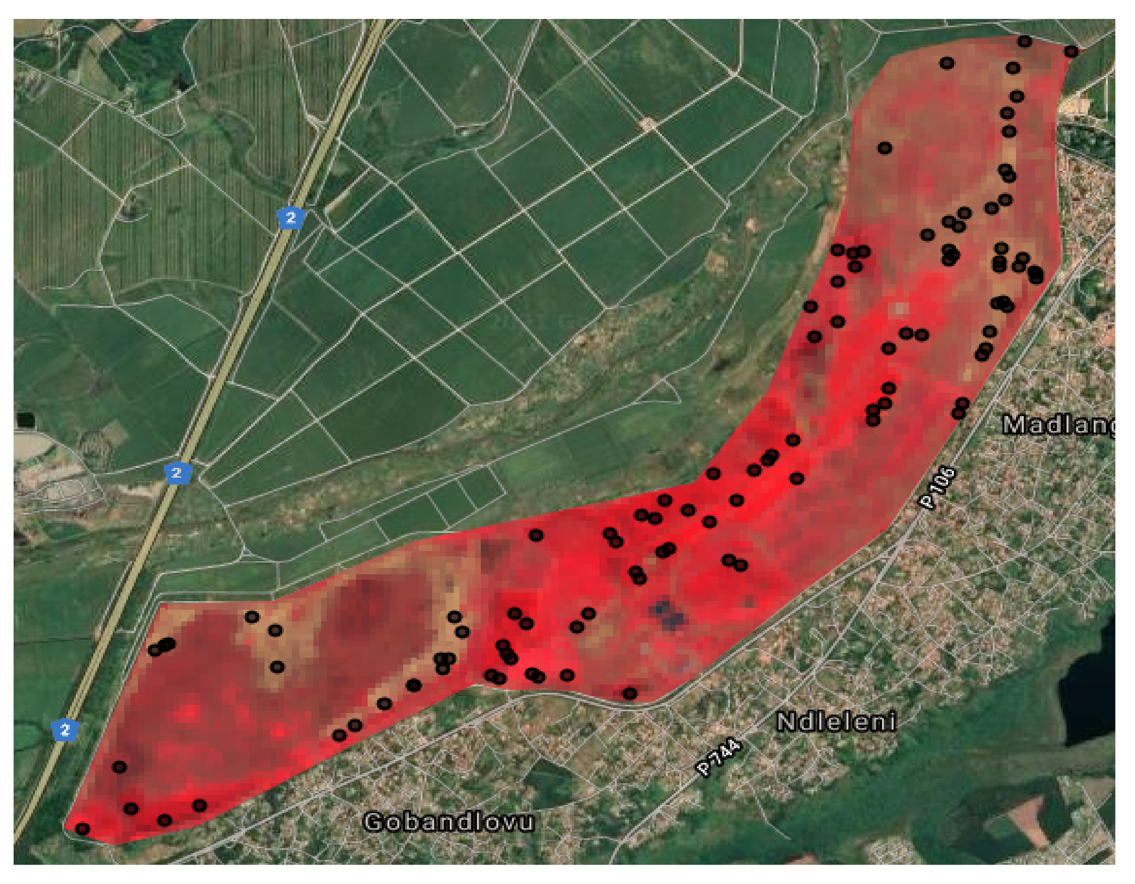
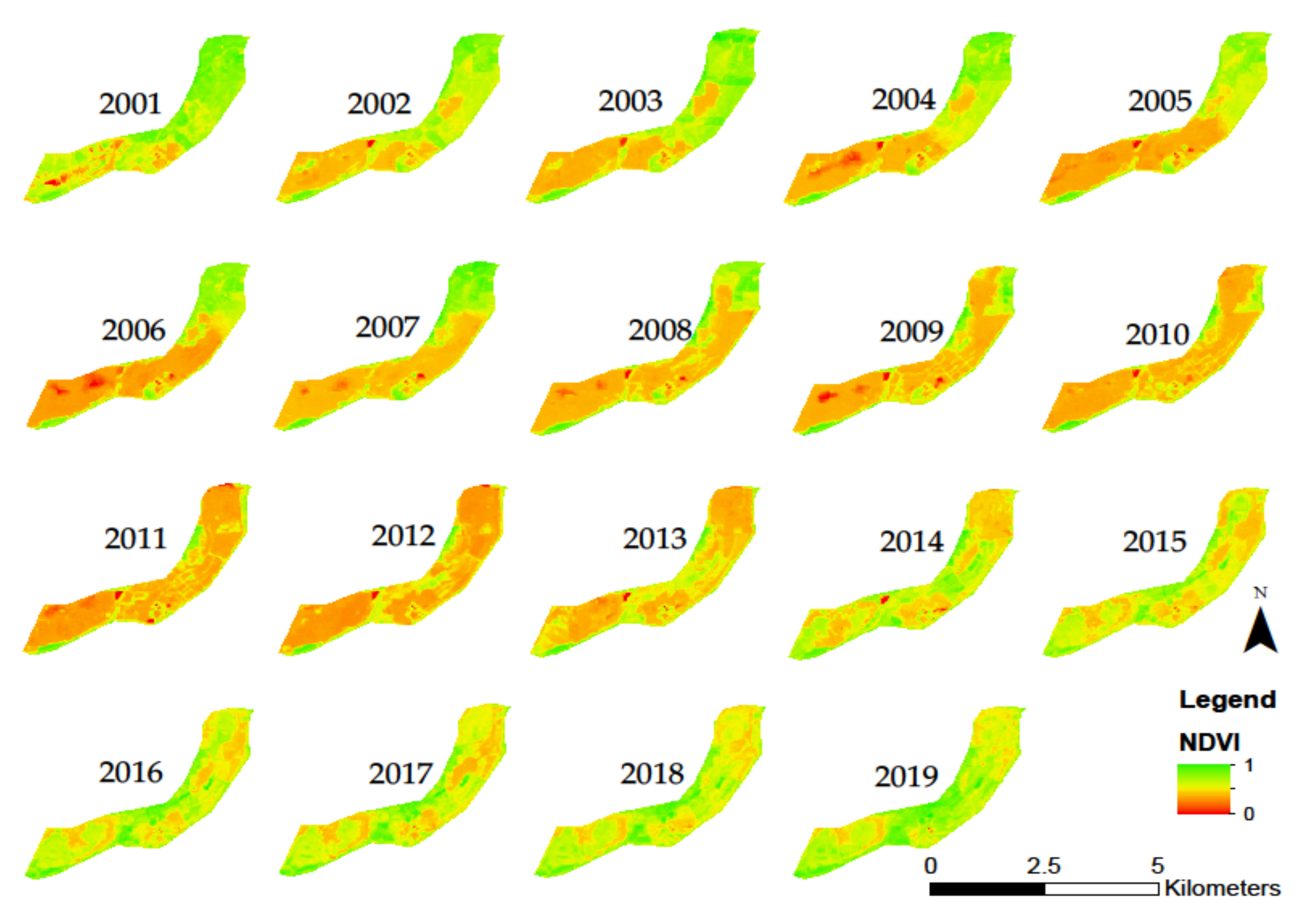
3.1. Spatiotemporal Patterns of Mine-Induced Disturbance and Recovery

It is worth noting that the extraction operations started in 2001 and ceased in 2013. Here, we began the analysis in the year 2000 as a benchmark to observe progressions of vegetation disturbance until 2013, after which rehabilitation was implemented. The results showing NDVI maps of the Hillendale mine obtained from 2000 through to 2019 are displayed in Figure 5. As expected, the Hillendale mining area was dominated by vegetation with varying NDVI signals in 2000, and this is partly attributable to various classes that were dominated by commercial sugarcane plantations. In 2001, the appearance of considerable mining activity was notable, with reduced NDVI values visible over the southern sections of the study area. From 2002 to 2013, the continuous decline of NDVI signifying progressions of mining severity is apparent.

We observed a substantial improvement of NDVI from 2014 to 2019, although some bare patches were disappearing slightly through this time. According to Beukes et al. [5], the restoration process is ongoing as most activities have been accomplished. The remaining process will require some time since the growth of the Eucalyptus trees is expected to increase the vegetation coverage as they mature. This process is projected to stabilize the site to ensure that the closure requirements are met. The recovery pattern remains on a trajectory towards a vegetation-dominated site from a remote sensing perspective but is yet to reach full recovery for the NDVI. Overall, our results show that the rehabilitation of the Hillendale mine has not yet reached its final state; however, they indicate satisfactory growth and are not inconsistent with the government restoration targets, and this sets a good precedent for the currently active Tronox Fairbreeze mining operation, which has a similar background.

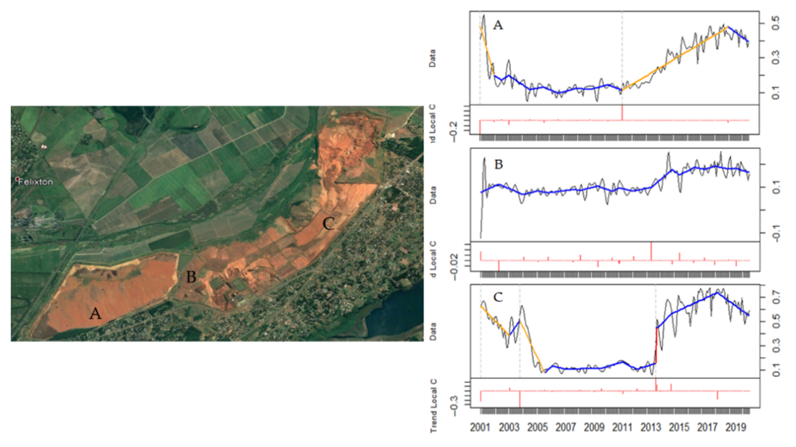
3.2. Overall and Site-Specific Trends of Disturbance and Recovery

We expanded the above analysis through a detailed examination of the overall NDVI time-series pattern of the Hillendale mine using the DBEST algorithm to give a complete picture of the disturbance and recovery dynamics from 2001 to 2019; the results are displayed in Figure 6. From this figure, the tendency of NDVI to form a V-shaped pattern is apparent. This pattern is expected for progressively recovering mining operations. Higher NDVI values dominate both the pre- and post-mining stages of its lifespan, with the lowest values during the peak of the process. The NDVI pattern over the Hillendale mine exhibited this trajectory; in 2001, the NDVI was 0.4, and it declined to 0.2 in 2009 until 2011. Subsequently, a recovering pattern is notable approaching 2019. Specifically, four key breakpoints related to devegetation are apparent from the figure, and their magnitude decreases in 2001, 2003, 2006, and 2010. On the other hand, breakpoints associated with revegetation are notable from 2011 and 2013, with the highest in 2015 and slightly lower in 2019—all pointing towards a successful rehabilitation program.

We further inspected the site-specific pixel trajectories for three sites within the operational area, and the outcome is presented in Figure 7. Site A represents the RSF—an earth-fill embankment facility formed by the disposal of residuals after extraction and beneficiation of the minerals [63], and is characterized by very fine-textured material and very high salinity, resulting in a much-reduced drainage capacity and leading to prolonged times for drying and stabilizing the substrate [64], as illustrated in Figure 8. As expected, lower NDVI values (~0.1) are apparent throughout the course of the mining operation until a marked increase in 2013 when the rehabilitation began. The vegetation planted on the RSF is doing well and successfully fulfills key objectives: drying the dam, suppressing dust, improving conditions for sugarcane production, and enabling the rehabilitation team to draw valuable lessons [65]. While the greater section of the RSF shows a good vegetation recovery pattern, the rest of the surface is being left to vegetate naturally, which it is doing successfully [41]. Site B indicates a relatively consistent NDVI pattern throughout the study period; however, a slight increment is noticeable from 2013. Site C exhibits a clear disturbance pattern in 2003–2004, with NDVI dropping from ~0.6 to 0.1 and remained low through to 2013, when a marked recovery to 0.5 transpired, forming an escarpment. A further increase of NDVI beyond 2013 is inspiring. These results show that the magnitude of disturbance is uneven within the mining site, and so is the temporal pattern of recovery rates; however, the overall picture signifies an effective reclamation.

Our results are consistent with Tronox [41] in that some sections of the mine have successful vegetation plots while some areas are less successful. The evidence highlighted by the cited work suggests that the ineffective plots may be attributable to a high water content, high sand content, or competition from other species, especially Phragmites in the RSF. The walls of the RSF are vegetated with indigenous grass to prevent surface erosion, as illustrated in Figure 8. Further, the experimental Eucalyptus and Casuarina trees established on the RSF and other mined areas show continuous success [41]. The Phragmites australis is the dominant species over the more extensive section of the RSF and is noticeably the best adapted to the conditions there [5].

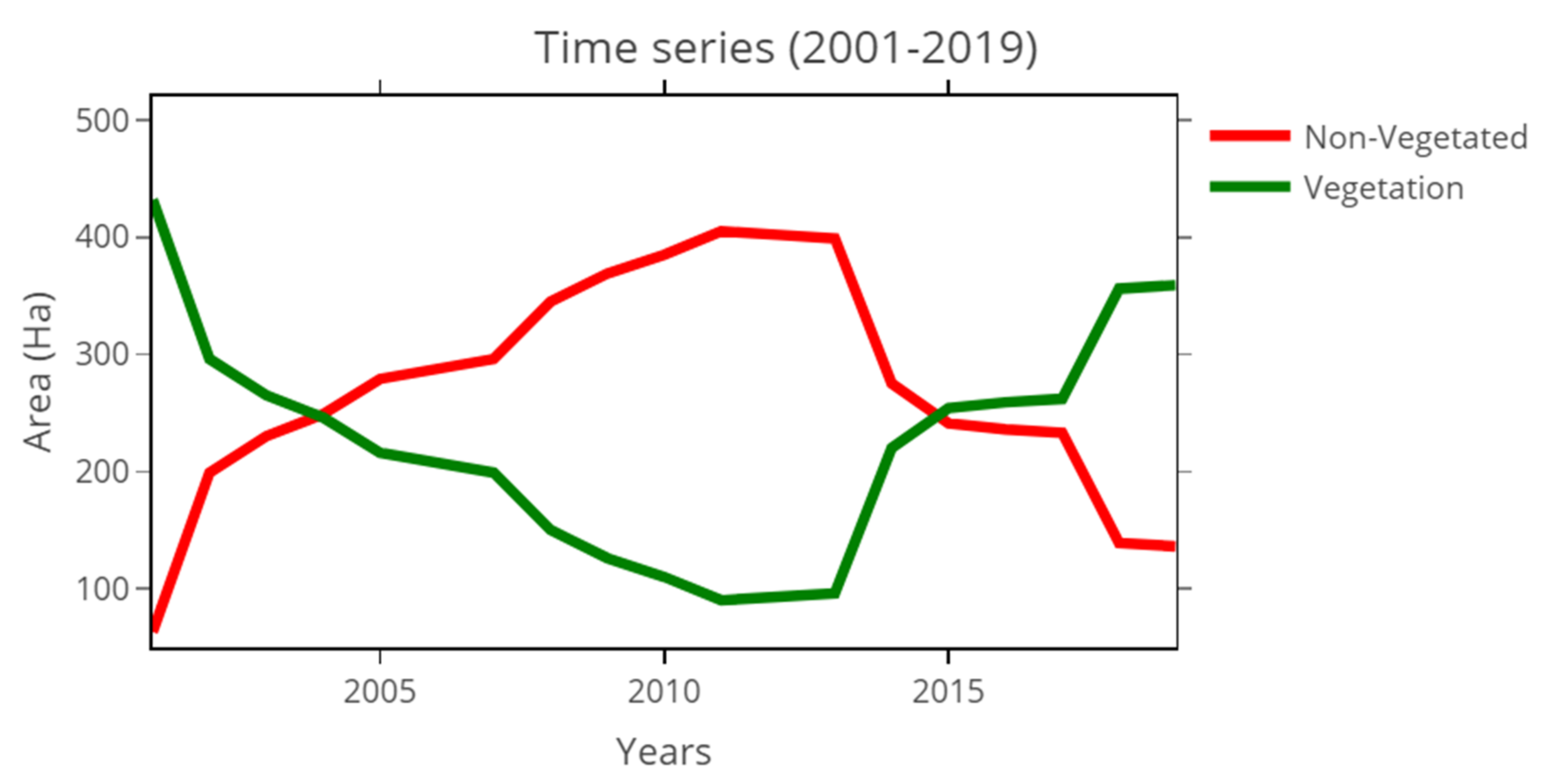
3.3. Areal Extent of Mining and Reclamation between 2001 and 2019

The annual averaged non-vegetated area and vegetated area for the period from 2001 to 2019 was computed for the study area (see Figure 9). The red line represents the non-vegetated area annual mean time series, while the green line represents the vegetated area. The non-vegetated time series increases from its initial value of 63 Ha in 2001 and reaches its maximum peak of 405 Ha in 2013. From 2013 onwards, it dropped to its lowest downward point at 136 Ha in 2019. This is presumably because the Tronox mine started its mining activities in 2001, which meant bare soil began to be exposed. In 2013, the largest portion of vegetation must have been removed, which is why the area of bare soil is at its highest. The vegetation begins to drop in 2001, with its lowest point being in the year 2013 with an area of 96 Ha, presumably due to the increase in mining activities in the study area. In 2013, it began to peak, reaching a maximum of 359 Ha in 2018.

For the purpose of the trend analysis of the non-vegetated and vegetated time series, MK and SQ-MK test methods were used. In terms of the MK trend test, the non-vegetated and vegetated time series were observed to have a z-score value of 0.28. This indicates an upwards but not significant trend in terms of the total time series. In order to determine the temporal dynamics of the trend, the SQ-MK test method was used. Figure 10 shows the sequential statistical values of forward/progressive (Prog) (solid redline) and retrograde (Retr) (solid blue line) obtained by the SQ-MK test for the annual mean of non-vegetated (a) and vegetated (b). In general, the SQ-MK statistic indicates a significant downward trend for vegetation and an upward trend for the non-vegetated area time series during the period from 2004 to 2016, with z-score values higher than +1.96 for the forward statistic (prog) of non-vegetated time series and lower than –1.96 for the forward statistic (prog) of vegetated time series. The change detection point is identified to be 2003 for non-vegetated and vegetation annual area times series, respectively. This is consistent with the earlier observation, which showed that vegetation was lost during the 2004–2016 period (the intense mining period). The recovery of the vegetation in the mine only started in 2013, which indicated the beginning of the rehabilitation phase.

3.4. Accuracy Assessment

We now consider to what extent our classification procedure separated the vegetated and non-vegetated areas within the Hillendale mine site. The overall accuracies of RF classification for mine disturbance and recovery varied slightly above 0.78 across the years from 2001 and 2019 (Figure 11). These accuracies are satisfactory and comparable with related mining studies. For example, Zhang et al. [66] achieved overall accuracies between 93% and 94% when they examined forest cover from 2006 to 2017 over mining, indicating a successful recovery in a mining region of Nanjing, Eastern China. Xiao et al. [37] also achieved high overall accuracies (0.81 and 0.84) of vegetation disturbance and reclamation from 2004 to 2019 over a surface coal mining region in the Shengli Coalfield in Inner Mongolia, China.

4. Discussion

The overall goal of rehabilitating mined-out areas is to restore the affected landscape conditions as closely as possible to their pre-mining reference state [67]; in our case, the Hillendale mine had a legal responsibility to restore its site to sustainable sugarcane production land use [40]. Here, we showcased the capacity of the DBEST algorithm to successfully track this development using Landsat and GEE resources. We observed an overall vegetation recovery pattern, pointing towards a successful rehabilitation, although not yet finalized. Similarly, Xiao et al. [37] used the LandTrendr algorithm within the GEE platform and successfully determined land reclamation in open-pit mining areas of a coalfield between 2003 and 2019.

Our results showed that the DBEST algorithm is highly capable of detecting breakpoints in the NDVI time series for the Hillendale mine area. The general reduction of NDVI until 2009–2011 and the recovery from 2013 reflects a continuation of the rehabilitation effort by the mine. In addition, our results reaffirmed the value of GEE-based algorithms for the rapid generation of products for tracking dynamics over mining landscapes. We found classification accuracies as high as 0.78 using the RF algorithm, and this was expected given the spectral contrast between mined-out and vegetated classes within the mining site. These results are consistent with Dlamini and Xulu [36]. The GEE-based resources have increased in use and importance for mining applications as they offer a fast and effective means for computing remotely sensed analysis. Despite this advantage, users are expected to have a basic understanding of programming.

While this approach is quick and affordable, several considerations should be taken into account. First, the use of Landsat data presents a challenge in problematic cloud regions. Second, the NDVI assessment must be placed in the proper context because it is based on NDVI values and not on-field evaluations [68]. The implication of this is that the status of reclamation is based only on vegetative cover and not on the actual vegetation species within the mining area. Therefore, there is a strong need for field verification or knowledge of the vegetation type responsible for the NDVI pattern. From an environmental perspective, the NDVI recovery results from alien plant species as natives may not be considered suitable. Our approach is disadvantaged by these methodological limitations.

5. Conclusions

In this study, the importance of time-series remote sensing analysis for characterizing mine-induced disturbance and restoration over the Tronox KZN Sands Hillendale mining site between 2001 and 2019 has been illustrated. Our results reveal a decreasing NDVI trend when the operation started in 2001 and deepens to the lowest point over the period 2009 to 2011, with a subsequent recovery coinciding with the cessation of operations and rehabilitation efforts noticeable from 2013 onwards. However, different sites are progressing at varying levels, and this is mainly due to the growth of diverse vegetation types within the site, which include sugarcane, reeds, and the Eucalyptus tree species. Furthermore, our random forests classification was capable of separating vegetated and non-vegetated areas within the affected area with accuracies exceeding 78%.

From this analysis, we conclude that the DBEST algorithm is a valuable tool for detecting patterns of disturbance and restoration over surface mining environments, especially Hillendale. Our study showed uneven recovery patterns for selected sites within the mining site; however, the overall picture indicates an effective restoration. Moreover, our affordable approach can better extract mine-induced disturbance and restoration patterns with a high degree of fidelity and be replicable in many areas undergoing intense vegetation transformations, particularly in data-poor countries with limited resources. We suggest, however, that a complete translation of the DBEST algorithm code into a GEE platform could enhance its application as it would be more easily accessible for the broader community.

References

1. Jones, J.V., III; Piatak, N.M.; Bedinger, G.M. Zirconium and Hafnium; US Geological Survey: Reston, VA, USA, 2017. [Google Scholar]
2. Omphemetse, M. An Overview of South Africa’s Zircon Industry and the Role of BEE; Department of Mineral Resources: Pretoria, South Africa, 2007. [Google Scholar]
3. Harlow, K. Naturally Occurring Radioactive Materials and the Regulatory Challenges to the Zircon Industry. J. S. Afr. Inst. Min. Metall. 2017, 117, 409–413. [Google Scholar] [CrossRef] [Green Version]
4. Tyler, R.M.; Minnitt, R.C.A. A Review of Sub-Saharan Heavy Mineral Sand Deposits: Implications for New Projects in Southern Africa. J. S. Afr. Inst. Min. Metall. 2004, 104, 89–99. [Google Scholar]
5. Beukes, J.A.; Vlok, M.L.; Khosa, F.E. Rehabilitation of the Hillendale Mine’s Residue Storage Facility. In Proceedings of the 22nd International Conference on Paste, Thickened and Filtered Tailings, Cape Town, South Africa, 8–10 May 2019; Australian Centre for Geomechanics: Crawley, WA, Australia, 2019; pp. 467–478. [Google Scholar]
6. Limpitlaw, D.; Aken, M.; Lodewijks, H.; Viljoen, J. Post-Mining Rehabilitation, Land Use and Pollution at Collieries in South Africa. In Proceedings of the Colloquium: Sustainable Development in the Life of Coal Mining; South African Institute of Mining and Metallurgy: Boksburg, South Africa, 2005; Volume 13. [Google Scholar]
7. Rîșteiu, N.T.; Creţan, R.; O’Brien, T. Contesting Post-Communist Economic Development: Gold Extraction, Local Community, and Rural Decline in Romania. Eurasian Geogr. Econ. 2021, 1–23. [Google Scholar] [CrossRef]
8. Mansur, I. Integrating Biodiversity Conservation and Agricultural Production in Mine Reclamation for Sustainable Development. J. Dev. Sustain. Agric. 2012, 7, 97–102. [Google Scholar]
9. Dick, L. Butchart Gardens. Public Hist. 2004, 26, 88–90. [Google Scholar] [CrossRef]
10. Cornelissen, H.; Watson, I.; Adam, E.; Malefetse, T. Challenges and Strategies of Abandoned Mine Rehabilitation in South Africa: The Case of Asbestos Mine Rehabilitation. J. Geochem. Explor. 2019, 205, 106354. [Google Scholar] [CrossRef]
11. Kuter, N. Reclamation of degraded landscapes due to opencast mining. In Advances in Landscape Architecture; IntechOpen: London, UK, 2013. [Google Scholar]
12. Hirons, M.; Hilson, G.; Asase, A.; Hodson, M.E. Mining in a Changing Climate: What Scope for Forestry-Based Legacies? J. Clean. Prod. 2014, 84, 430–438. [Google Scholar] [CrossRef]
13. Kobayashi, H.; Watando, H.; Kakimoto, M. A Global Extent Site-Level Analysis of Land Cover and Protected Area Overlap with Mining Activities as an Indicator of Biodiversity Pressure. J. Clean. Prod. 2014, 84, 459–468. [Google Scholar] [CrossRef] [Green Version]
14. Murguía, D.I.; Bringezu, S.; Schaldach, R. Global Direct Pressures on Biodiversity by Large-Scale Metal Mining: Spatial Distribution and Implications for Conservation. J. Environ. Manag. 2016, 180, 409–420. [Google Scholar] [CrossRef] [PubMed]
15. Hodge, R.A. Mining Company Performance and Community Conflict: Moving beyond a Seeming Paradox. J. Clean. Prod. 2014, 84, 27–33. [Google Scholar] [CrossRef]
16. De Simoni, B.S.; Leite, M.G.P. Assessment of Rehabilitation Projects Results of a Gold Mine Area Using Landscape Function Analysis. Appl. Geogr. 2019, 108, 22–29. [Google Scholar] [CrossRef]
17. Hancock, G.R.; Lowry, J.B.C.; Coulthard, T.J. Long-Term Landscape Trajectory—Can We Make Predictions about Landscape Form and Function for Post-Mining Landforms? Geomorphology 2016, 266, 121–132. [Google Scholar] [CrossRef]
18. Karan, S.K.; Samadder, S.R.; Maiti, S.K. Assessment of the Capability of Remote Sensing and GIS Techniques for Monitoring Reclamation Success in Coal Mine Degraded Lands. J. Environ. Manag. 2016, 182, 272–283. [Google Scholar] [CrossRef] [PubMed]
19. Department of Mineral Resources. RSA Mineral and Petroleum Resources Development Act No. 28 of 2002; Department of Mineral Resources: Pretoria, South Africa, 2002. [Google Scholar]
20. Van Zyl, H.; Bond-Smith, M.; Minter, T.; Botha, M.; Leiman, A. Financial Provisions for Rehabilitation and Closure in South African Mining: Discussion Document on Challenges and Recommended Improvements. WWF–South Africa. 2012. Available online: http://awsassets.wwf.org.za/downloads/summary_mining_report_8aug.pdf (accessed on 7 January 2021).
21. Hattingh, R.P.; Beukes, I.; Krause, B.; Kotze, H. Soil Reconstitution as a Key Driver for Successful Rehabilitation at Hillendale Mine. In Proceedings of the 6th International Heavy Minerals Conference ‘Back to Basics’; Southern African Institute of Mining and Metallurgy: Johannesburg, South Africa , 2007; pp. 31–34. [Google Scholar]
22. Ruiz-Jaen, M.C.; Mitchell Aide, T. Restoration Success: How Is It Being Measured? Restor. Ecol. 2005, 13, 569–577. [Google Scholar] [CrossRef]
23. Vogelmann, J.E.; Gallant, A.L.; Shi, H.; Zhu, Z. Perspectives on Monitoring Gradual Change across the Continuity of Landsat Sensors Using Time-Series Data. Remote Sens. Environ. 2016, 185, 258–270. [Google Scholar] [CrossRef] [Green Version]
24. Yuan, Y.; Zhao, Z.; Niu, S.; Li, X.; Wang, Y.; Bai, Z. Reclamation Promotes the Succession of the Soil and Vegetation in Opencast Coal Mine: A Case Study from Robinia Pseudoacacia Reclaimed Forests, Pingshuo Mine, China. Catena 2018, 165, 72–79. [Google Scholar] [CrossRef]
25. Wang, J.; Wang, H.; Cao, Y.; Bai, Z.; Qin, Q. Effects of Soil and Topographic Factors on Vegetation Restoration in Opencast Coal Mine Dumps Located in a Loess Area. Sci. Rep. 2016, 6, 22058. [Google Scholar] [CrossRef] [Green Version]
26. Lechner, A.M.; McIntyre, N.; Witt, K.; Raymond, C.M.; Arnold, S.; Scott, M.; Rifkin, W. Challenges of Integrated Modelling in Mining Regions to Address Social, Environmental and Economic Impacts. Environ. Model. Softw. 2017, 93, 268–281. [Google Scholar] [CrossRef]
27. Whiteside, T.G.; Bartolo, R.E. A Robust Object-Based Woody Cover Extraction Technique for Monitoring Mine Site Revegetation at Scale in the Monsoonal Tropics Using Multispectral RPAS Imagery from Different Sensors. Int. J. Appl. Earth Obs. Geoinformation 2018, 73, 300–312. [Google Scholar] [CrossRef]
28. Bhandari, A.K.; Kumar, A.; Singh, G.K. Feature Extraction Using Normalized Difference Vegetation Index (NDVI): A Case Study of Jabalpur City. Procedia Technol. 2012, 6, 612–621. [Google Scholar] [CrossRef] [Green Version]
29. Hunt Jr, E.R.; Doraiswamy, P.C.; McMurtrey, J.E.; Daughtry, C.S.; Perry, E.M.; Akhmedov, B. A Visible Band Index for Remote Sensing Leaf Chlorophyll Content at the Canopy Scale. Int. J. Appl. Earth Obs. Geoinf. 2013, 21, 103–112. [Google Scholar] [CrossRef] [Green Version]
30. Tucker, C.J. Red and Photographic Infrared Linear Combinations for Monitoring Vegetation. Remote Sens. Environ. 1979, 8, 127–150. [Google Scholar] [CrossRef] [Green Version]
31. Murillo-Sandoval, P.J.; Hilker, T.; Krawchuk, M.A.; Van Den Hoek, J. Detecting and Attributing Drivers of Forest Disturbance in the Colombian Andes Using Landsat Time-Series. Forests 2018, 9, 269. [Google Scholar] [CrossRef] [Green Version]
32. Kennedy, R.E.; Yang, Z.; Cohen, W.B. Detecting Trends in Forest Disturbance and Recovery Using Yearly Landsat Time Series: 1. LandTrendr—Temporal Segmentation Algorithms. Remote Sens. Environ. 2010, 114, 2897–2910. [Google Scholar] [CrossRef]
33. Verbesselt, J.; Hyndman, R.; Newnham, G.; Culvenor, D. Detecting Trend and Seasonal Changes in Satellite Image Time Series. Remote Sens. Environ. 2010, 114, 106–115. [Google Scholar] [CrossRef]
34. Wang, E.; Wang, X.; Chen, Y. The Breakpoints Detection Method Using Time Series of Vegetation Fractional Coverage. J. Geo-inf. Sci. 2017, 19, 1355–1363. [Google Scholar]
35. Jamali, S.; Jönsson, P.; Eklundh, L.; Ardö, J.; Seaquist, J. Detecting Changes in Vegetation Trends Using Time Series Segmentation. Remote Sens. Environ. 2015, 156, 182–195. [Google Scholar] [CrossRef]
36. Dlamini, L.Z.; Xulu, S. Monitoring Mining Disturbance and Restoration over RBM Site in South Africa Using Landtrendr Algorithm and Landsat Data. Sustainability 2019, 11, 6916. [Google Scholar] [CrossRef] [Green Version]
37. Xiao, W.; Deng, X.; He, T.; Chen, W. Mapping Annual Land Disturbance and Reclamation in a Surface Coal Mining Region Using Google Earth Engine and the LandTrendr Algorithm: A Case Study of the Shengli Coalfield in Inner Mongolia, China. Remote Sens. 2020, 12, 1612. [Google Scholar] [CrossRef]
38. Ang, M.L.E.; Arts, D.; Crawford, D.; Labatos, B.V., Jr.; Ngo, K.D.; Owen, J.R.; Gibbins, C.; Lechner, A.M. Socio-Environmental Land Cover Time-Series Analysis of Mining Landscapes Using Google Earth Engine and Web-Based Mapping. Remote Sens. Appl. Soc. Environ. 2021, 21, 100458. [Google Scholar]
39. He, T.; Xiao, W.; Zhao, Y.; Chen, W.; Deng, X.; Zhang, J. Continues Monitoring of Subsidence Water in Mining Area from the Eastern Plain in China from 1986 to 2018 Using Landsat Imagery and Google Earth Engine. J. Clean. Prod. 2021, 279, 123610. [Google Scholar] [CrossRef]
40. Van Jaarsveld, C.M. Rehabilitation of Mined-out Dune Land at Tronox KZN Sands for Sugarcane Production. Ph.D. Thesis, University of the Free State, Bloemfontein, South Africa, 2013. [Google Scholar]
41. Tonox Environmental Legal Compliance Audit Tronox KZN. Available online: https://www.tronox.com/download.php?path=14885 (accessed on 29 April 2021).
42. Roy, D.P.; Wulder, M.A.; Loveland, T.R.; Woodcock, C.E.; Allen, R.G.; Anderson, M.C.; Helder, D.; Irons, J.R.; Johnson, D.M.; Kennedy, R. Landsat-8: Science and Product Vision for Terrestrial Global Change Research. Remote Sens. Environ. 2014, 145, 154–172. [Google Scholar] [CrossRef] [Green Version]
43. Halabisky, M.; Babcock, C.; Moskal, L.M. Harnessing the Temporal Dimension to Improve Object-Based Image Analysis Classification of Wetlands. Remote Sens. 2018, 10, 1467. [Google Scholar] [CrossRef] [Green Version]
44. Geng, L.; Ma, M.; Wang, H. An Effective Compound Algorithm for Reconstructing MODIS NDVI Time Series Data and Its Validation Based on Ground Measurements. IEEE J. Sel. Top. Appl. Earth Obs. Remote Sens. 2015, 9, 3588–3597. [Google Scholar] [CrossRef]
45. Jamali, S.; Tomov, H. DBEST: Detecting Breakpoints and Estimating Segments in Trend. Available online: https://rdrr.io/cran/DBEST/man/DBEST.html (accessed on 1 March 2021).
46. Goldblatt, R.; You, W.; Hanson, G.; Khandelwal, A.K. Detecting the Boundaries of Urban Areas in India: A Dataset for Pixel-Based Image Classification in Google Earth Engine. Remote Sens. 2016, 8, 634. [Google Scholar] [CrossRef] [Green Version]
47. Alonso, A.; Muñoz-Carpena, R.; Kennedy, R.E.; Murcia, C. Wetland Landscape Spatio-Temporal Degradation Dynamics Using the New Google Earth Engine Cloud-Based Platform: Opportunities for Non-Specialists in Remote Sensing. Trans. ASABE 2016, 59, 1331–1342. [Google Scholar]
48. Gorelick, N.; Hancher, M.; Dixon, M.; Ilyushchenko, S.; Thau, D.; Moore, R. Google Earth Engine: Planetary-Scale Geospatial Analysis for Everyone. Remote Sens. Environ. 2017, 202, 18–27. [Google Scholar] [CrossRef]
49. Kumar, L.; Mutanga, O. Google Earth Engine Applications since Inception: Usage, Trends, and Potential. Remote Sens. 2018, 10, 1509. [Google Scholar] [CrossRef] [Green Version]
50. Zhao, Y.; Gong, P.; Yu, L.; Hu, L.; Li, X.; Li, C.; Zhang, H.; Zheng, Y.; Wang, J.; Zhao, Y. Towards a Common Validation Sample Set for Global Land-Cover Mapping. Int. J. Remote Sens. 2014, 35, 4795–4814. [Google Scholar] [CrossRef]
51. Breiman, L. Random Forests. Mach. Learn. 2001, 45, 5–32. [Google Scholar] [CrossRef] [Green Version]
52. Kohavi, R. A Study of Cross-Validation and Bootstrap for Accuracy Estimation and Model Selection. In Proceedings of the IJCAI, Montreal, QC, Canada, 20–25 August 1995; Volume 14, pp. 1137–1145. [Google Scholar]
53. Gómez, C.; White, J.C.; Wulder, M.A. Optical Remotely Sensed Time Series Data for Land Cover Classification: A Review. ISPRS J. Photogramm. Remote Sens. 2016, 116, 55–72. [Google Scholar] [CrossRef] [Green Version]
54. Fernández-Delgado, M.; Cernadas, E.; Barro, S.; Amorim, D. Do We Need Hundreds of Classifiers to Solve Real World Classification Problems? J. Mach. Learn. Res. 2014, 15, 3133–3181. [Google Scholar]
55. Foody, G.M. Assessing the Accuracy of Land Cover Change with Imperfect Ground Reference Data. Remote Sens. Environ. 2010, 114, 2271–2285. [Google Scholar] [CrossRef] [Green Version]
56. Kendall, M.G.; Gibbons, J.D. Rank Correlation Methods, 1970; Griffin: London, UK, 1975. [Google Scholar]
57. Mann, H.B. Nonparametric Tests against Trend. Econom. J. Econom. Soc. 1945, 13, 245–259. [Google Scholar] [CrossRef]
58. Gilbert, R.O. Statistical Methods for Environmental Pollution Monitoring; John Wiley & Sons: Hoboken, NJ, USA, 1987. [Google Scholar]
59. Sneyers, R. On the Statistical Analysis of Series of Observations; WMO: Geneva, Switzerland, 1991. [Google Scholar]
60. Mosmann, V.; Castro, A.; Fraile, R.; Dessens, J.; Sanchez, J.L. Detection of Statistically Significant Trends in the Summer Precipitation of Mainland Spain. Atmos. Res. 2004, 70, 43–53. [Google Scholar] [CrossRef]
61. Zarenistanak, M.; Dhorde, A.G.; Kripalani, R.H. Trend Analysis and Change Point Detection of Annual and Seasonal Precipitation and Temperature Series over Southwest Iran. J. Earth Syst. Sci. 2014, 123, 281–295. [Google Scholar] [CrossRef]
62. Mbatha, N.; Xulu, S. Time Series Analysis of MODIS-Derived NDVI for the Hluhluwe-Imfolozi Park, South Africa: Impact of Recent Intense Drought. Climate 2018, 6, 95. [Google Scholar] [CrossRef] [Green Version]
63. Festin, E.S.; Tigabu, M.; Chileshe, M.N.; Syampungani, S.; Odén, P.C. Progresses in Restoration of Post-Mining Landscape in Africa. J. For. Res. 2019, 30, 381–396. [Google Scholar] [CrossRef] [Green Version]
64. Shaygan, M.; Usher, B.; Baumgartl, T. Modelling Hydrological Performance of a Bauxite Residue Profile for Deposition Management of a Storage Facility. Water 2020, 12, 1988. [Google Scholar] [CrossRef]
65. Tronox The Yellow Machines Are Moving: The Construction Suspension Has Been Lifted and the Fairbreeze Site Is Humming. Available online: https://words-worth.co.za/words-worth/downloads/portfolio/2014/fairtalk13_2014.pdf (accessed on 15 April 2021).
66. Zhang, Y.; Shen, W.; Li, M.; Lv, Y. Integrating Landsat Time Series Observations and Corona Images to Characterize Forest Change Patterns in a Mining Region of Nanjing, Eastern China from 1967 to 2019. Remote Sens. 2020, 12, 3191. [Google Scholar] [CrossRef]
67. Balaguer, L.; Escudero, A.; Martín-Duque, J.F.; Mola, I.; Aronson, J. The Historical Reference in Restoration Ecology: Re-Defining a Cornerstone Concept. Biol. Conserv. 2014, 176, 12–20. [Google Scholar] [CrossRef]
68. Yang, Z.; Li, J.; Zipper, C.E.; Shen, Y.; Miao, H.; Donovan, P.F. Identification of the Disturbance and Trajectory Types in Mining Areas Using Multitemporal Remote Sensing Images. Sci. Total Environ. 2018, 644, 916–927. [Google Scholar] [CrossRef] [PubMed]
Figure 1. Location of Tronox KZN Sands Hillendale mine on the northeast coast of KwaZulu-Natal, South Africa.
Land 10 00760 g001
Figure 2. Flowchart of the methodology used in this study.
Land 10 00760 g002
Figure 3. Typical output of the DBEST change detection algorithm. The black line represents the NDVI time series, the blue line represents the estimation of the trend element, the red denotes abrupt change, and the orange represents gradual change. Below the time series trajectory is the local trend change with red bars characterizing the magnitude of breakpoints in the time series.
Land 10 00760 g003
Figure 4. Spatial distribution of samples for mined-out and vegetated areas within the Hillendale mine site.
Land 10 00760 g004
Figure 5. Spatiotemporal variability of normalized difference vegetation index (NDVI) over the Hillendale mine site (2001–2019). The scale denotes the range of NDVI values from 0 to 1. Orange values are associated with non-vegetated areas, whereas green is related to vegetated areas.
Land 10 00760 g005
Figure 6. The DBEST breakpoint detection of the overall NDVI time series over the Hillendale mine (2001–2019).
Land 10 00760 g006
Figure 7. (AC) The DBEST NDVI trends in selected sites within the Hillendale mining site.
Land 10 00760 g007
Figure 8. Placing of grass on the walls of the residue storage facility (Source: Beukes et al. [5]).
Land 10 00760 g008
Figure 9. Time series of the total area of non-vegetated (red) and vegetation (green) within the Hillendale mine site over the period 2001 to 2019.
Land 10 00760 g009
Figure 10. Sequential Mann–Kendall analysis of the annual trend of non-vegetated (a) and the vegetated area within the Hillendale mine site (b). The red curve denotes the forward sequential values of the statistic u(t), and the blue curve denotes the backward sequential values of the statistics.
Land 10 00760 g010
Figure 11. Overall accuracies for each year between 2001 and 2019.
Land 10 00760 g011
Publisher’s Note: MDPI stays neutral with regard to jurisdictional claims in published maps and institutional affiliations.