Assessing Matching Characteristics and Spatial Differences between Supply and Demand of Ecosystem Services: A Case Study in Hangzhou, China

Abstract

Ecosystem services (ESs) is a term used to describe the foundations of the well-being of human society, and several relevant studies have been carried out in this area. However, given the fact that the complex trade-offs/synergy relationships of ESs are a challenging area, studies on matching mechanisms for ES supply and demand are still rare. In this study, using the InVEST model, ArcGIS, and other professional tools, we first mapped and quantitatively evaluated the supply and demand of five ES types (water yield, soil conservation, carbon retention, food supply, and leisure and entertainment) in Hangzhou, China, based on land use, meteorology, soil, and socio-economic data. Then, we analyzed the matching characteristics between the supply and demand of these ESs and analyzed the complex trade-offs and synergy between the supply and demand of ESs and factors affecting ESs. The results of this analysis indicate that although the ES supply and demand of carbon retention tended to be out of balance (supply was less than demand), the supply and demand of the other four ES types (i.e., water yield, soil conservation, food supply, and leisure and entertainment) were in balance (supply exceeded demand). Finally, the spatial heterogeneity of the supply and demand of ESs in Hangzhou was significant, especially in urban areas in the northeast and mountainous areas in the southwest. The supply of ESs was based on trade-offs, whereas the demand of ESs was based on synergy. Our results further show that the supply and demand of ESs in the urban area in Hangzhou were out of balance, whereas the supply and demand of ESs in the western region were coordinated. Therefore, the linkage of ES flows between this urban area and the western region should be strengthened. This innovative study could provide useful information for regional land use planning and environmental protection.

1. Introduction

Ecosystem services (ESs) refer to various benefits that mankind obtains directly or indirectly from ecosystems, maintaining the material foundations and environmental conditions on which mankind depends for survival and development. ESs are usually divided into four categories: supply, regulation, support, and cultural services [1,2,3]. In the context of rapid global urbanization, the intensity of human activities and land use in cities and rural areas has continued to increase, and the contradiction between man and land has become increasingly acute [4,5,6]. This has led to a degradation of regional ecological functions, an imbalance in ES supply and demand, and a series of ecological and environmental problems [7,8,9]. Therefore, the quantitative evaluation of regional ES capabilities and the identification of a relationship between the supply and demand of ecosystem services are high-priority and urgent tasks in current ecosystem science [10].

ES supply refers to the basic production and living services provided by a regional ecosystem to humans, including material data products and leisure and entertainment services, whereas ES demand refers to the human consumption and use of products and services provided by the ecosystem [7,11]. These two factors together constitute a dynamic process in which ESs flow from natural ecosystems to human social systems. Early research on ESs focused on regional ecosystem supply services, including the definition of regional ecosystem structure, functions, and related ES concepts, as well as the improvement of research frameworks, paying less attention to ecosystem demand services [7,12,13]. For example, Costanza et al. [1,14] put forward an organic combination of human activities, regional ecological environment, and global environmental changes to assess regional ecosystem health, as well as defining the concept of ES value and unifying the ESs of different species in relation to economic value. Davies et al. [15] investigated the distribution of vegetation in the City of Leicester in the UK and studied the amount and spatial pattern of carbon storage above the city. With the rapid advancement of industrialization and urbanization, traces of human activities continue to expand to natural land, such as forest, grassland, and water areas, leading to profound land cover changes at a regional scale, with cascade effects on the supply and demand of ESs [16,17,18]. Therefore, the evaluation of ecosystem supply and demand services is a current research hotspot in the academic community and in government departments, with particular regard to the quantitative assessment of regional ecosystem supply and demand services and spatial-temporal differences [19].

With the introduction and development of the Millennium Ecosystem Assessment (MA), many scholars throughout the world have carried out basic and applied research projects on the supply and demand of ESs, including the classification of supply and demand types, quantitative assessments, scale effects, assessments of spatial-temporal differences, and trade-offs/synergy analysis of the supply and demand of ESs, etc. [19,20]. Considering that a variety of ESs exhibit trade-off relationships and mutually-promoting synergistic relationships under the interaction of a set of complex influencing factors, relevant scholars have studied the spatial-temporal performance characteristics and formation mechanisms of ES trade-offs/synergy relationships [21]. For example, Sun et al. [22] estimated the carbon retention and food supply of the Yangtze River Delta Urban Agglomeration (YRDUA) from 2000 to 2010 and analyzed the trade-offs and synergy of ESs. Their results were able to provide comprehensive information for the management and decision-making in relation to ESs. Kragt and Robertson [23] revealed the trade-off relationships existing between Australia’s ESs, linking ESs to actual agricultural production. Quantifying the supply–demand ratio of ESs, changes in the supply and demand of ESs at different time and space scales, and studies of balance are also focus of current ES supply and demand research [24]. The ES supply and demand matrix proposed by Burkhard et al. [25] is easy to operate and has potential applicability. It has been widely used in the research of ES supply and demand in Europe and North America [25]. In addition, based on various research methods, such as land use change, ecological process simulation, expert experience discrimination, the InVEST model, the ARIES model, and spatial measurement models, etc., experts and scholars from different disciplines have evaluated the supply and demand situation of ecosystems at different scales, including at global, national, regional, and watershed levels [26,27,28]. The InVEST model, jointly developed by Stanford University, the Nature Conservancy (TNC), and the World Wildlife Fund (WWF), is widely used in the assessment of ecosystem services, such as habitat risk assessment, habitat quality, carbon, water yield, SDR, NDR, and many other modules for ESs [5]. Models have also been used to calculate ecosystem services quantitatively and valuably, outputting results in map form, displaying the spatial distribution of ESs, and carrying out ES evaluation simulations and trade-off analysis under different land use and cover types. Benra et al. [29] evaluated the performance of the InVEST seasonal water production model based on the water monitoring records of 224 catchments in southern Chile. González-García et al. [30] also used the InVEST model to evaluate changes in the supply and demand of water provisions, climate regulation, and outdoor recreation in the Madrid area (Spain).

At present, driven by rapid industrialization and urbanization, China’s economic society and ecological environment are undergoing significant changes. Consequently, a large number of research projects on ESs have been conducted in China [5,27]. However, there are also problems, such as the imperfect development of ES theory and unsound research methods, and the question of how to evaluate regional ES capabilities more accurately requires a lot of theory and practice [31]. Therefore, it is necessitary to quantitatively evaluate regional ecosystem supply and demand services and understand the difference between regional ES supply and demand, so as to improve the supply and service capabilities of a ecosystems in certain areas and to promote the balanced development of regional ES supply and demand [19,26]. It is also a key step required for ES to transition from theoretical research into management practice, which can help improve the efficiency of ecosystem management and realize the “win–win” situation of regional economic development and environmental protection [25,32].

As one of core cities in China’s Yangtze River Delta urban agglomeration, Hangzhou has hosted major international events, such as the G20 Summit and World Environment Day. It has a high socio-economic status and its urbanization rate reached 77.4% in 2018 [17]. The expansion of construction land acts on regional ecosystem services, leading to complexity in the supply and demand of ESs. Therefore, research on the supply and demand of ESs in Hangzhou is of great significance to the sustainable development of the region’s social economy and ecological environment. In this study, based on Hangzhou’s land use, meteorological, soil, and socio-economic data, the supply and demand of Hangzhou’s ESs, including water yield, soil conservation, carbon retention, food supply, and leisure and entertainment, are evaluated. The matching and spatial differences between the supply and demand of ESs in Hangzhou are analyzed. The specific research objectives in this study were (1) to identify the supply and demand areas of various ESs; (2) to explore the structure of the supply and demand of ESs and gaps between supply and demand, to explain the quantity and spatial matching relationships between the supply and demand of ESs, and to reveal the differences between the supply and demand of ESs; and (3) to analyze the trade-offs/synergy between ES supply and demand, as well as to explore the factors influencing regional ESs. The novel significance of this study is that the research results can provide theoretical guidance for the sustainable development of the social economy and ecological environment in Hangzhou, China, and other core cities in the world.

2. Materials and Methods

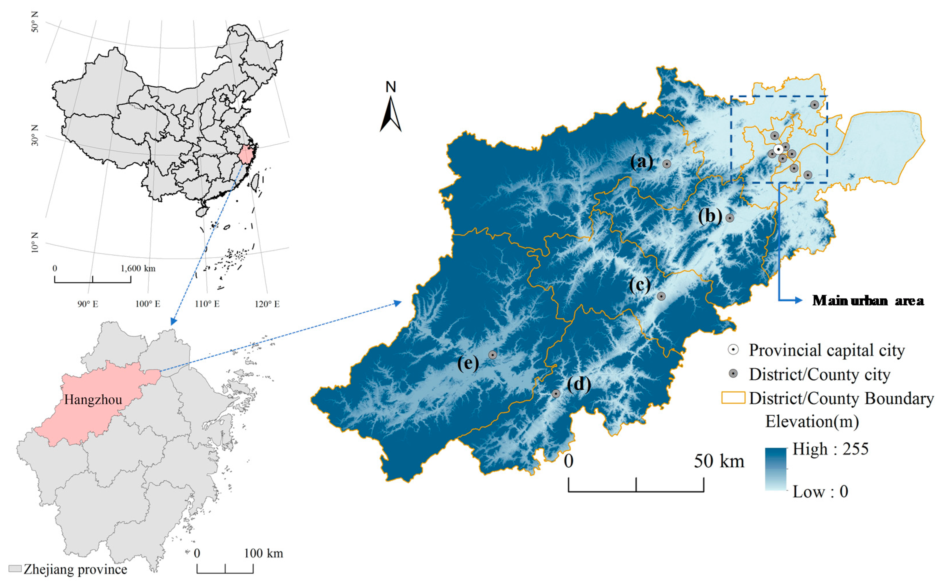
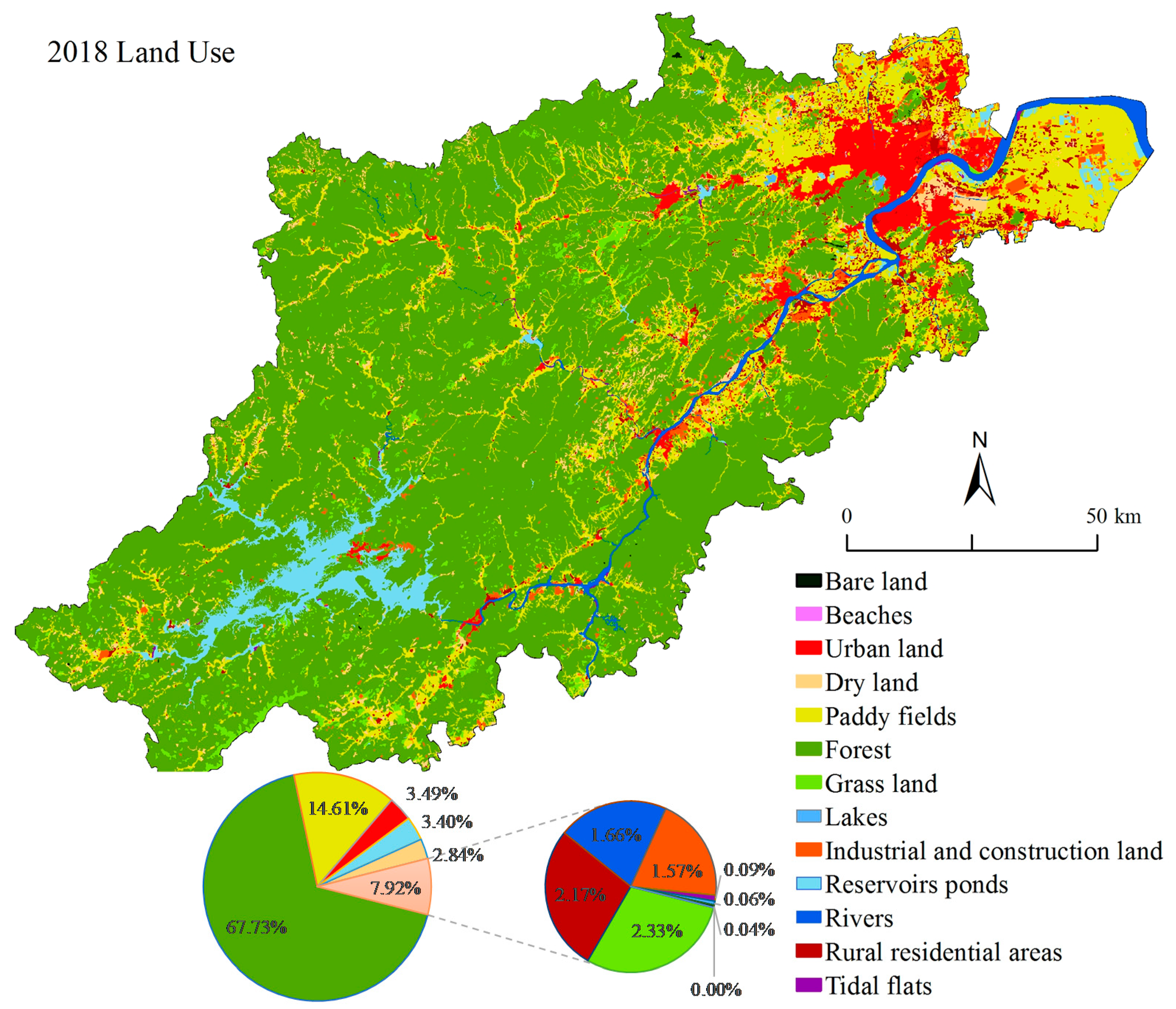
2.1. Study Area

The study area, Hangzhou, is located in the south wing of the Yangtze River Delta, northwestern Zhejiang Province, south of the Beijing–Hangzhou Grand Canal and east of the Hangzhou Bay (118°20′–120°37′ N and 29°11′–30°34′ E). Hangzhou consists of 13 counties and districts (10 municipal districts, two counties, and one county-level city), and it is not only one of the core cities in the Yangtze River Delta economic zone, but also the political, economic, cultural, and financial center of Zhejiang Province (Figure 1).

The terrain of Hangzhou is high in the west and low in the east, with a complex and diverse environment, integrating mountains, water bodies, and cities. The northeastern part belongs to the plain of northern Zhejiang, whereas the south, central, and western parts belong to the middle and low hills and hills of western Zhejiang, among which plains account for 26.4%; hills and mountains for 65.6%; and rivers, lakes, and reservoirs for 8%. Hangzhou is located in the transitional zone between central and north subtropical climates, with an average annual temperature of 15.3 °C–17 °C and an average annual precipitation of 1100–1600 mm. The main rivers are Qiantang River, East Tiaoxi, and the Beijing–Hangzhou Canal [17,33].

The administrative area of Hangzhou is about 16,858 km². By the end of 2018, the resident population reached 9.806 million, and the city’s GDP reached CNY 1350.92 billion, accounting for 26.79% of Zhejiang province’s GDP. With the rapid development of Hangzhou’s social economy, population surges, and the influx of the tourist population, the ecological system of Hangzhou will also be under increasing pressure in future.

2.2. Data Acquirement and Preparation

As shown in

Table A1. Description of the data used in this study.

Type of Dataset	Source	Processing	Format
Land use data	Resource and Environmental Science and Data Center of the Chinese Academy of Sciences (http://www.resdc.cn, accessed on 15 August 2020)	Extraction and reclassification	Raster (30 m)
Meteorological data	China Meteorological Data Network (http://data.cma.cn, accessed on 20 August 2020)	Kriging interpolation	Raster (30 m)
Soil data	Harmonized World Soil Database (HWSD)	Extraction and resampling	Raster (30 m)
Socio-economic data	Statistics Bureau of Hangzhou	Collection and summary	Excel
Basic geographic information data	China’s geospatial data cloud platform (http://www.gscloud.cn, accessed on 20 August 2020)	Mask extraction	Raster (30 m)Vector

, five categories of data were used in this study. The first category was land use data, obtained from the Resource and Environmental Science and Data Center of the Chinese Academy of Sciences (http://www.resdc.cn, accessed on 15 August 2020). The interpretation accuracy of these land use data is greater than 85% [34]. According to previous studies [34,35] and the requirements of the research area, land use was divided into 13 types, including dry land, paddy fields, forest, grassland, rivers, lakes, reservoirs ponds, tidal flats, beaches, urban land, rural residential areas, industrial and developed land, and bare land, as shown in Figure 1A. The second category of data was meteorological data, collected from the China Meteorological Data Network (http://data.cma.cn, accessed on 20 August 2020), which includes average temperature, average precipitation, and the regional potential evapotranspiration (PET) calculated using the Penman–Monteith formula [35]. We performed Kriging interpolation on the attribute data of the weather station to obtain the meteorological raster data (30 m). The third category of data was soil data, which came from the Harmonized World Soil Database (HWSD) [34,36]. The soil data were resampled to 30-m raster cells. The fourth category of data was socio-economic data, from the Zhejiang Statistical Yearbook and Hangzhou Statistical Yearbook (2018) [37], which were used to calculate per capita carbon emissions and food demand. We connected the attribute value of each indicator to the districts/counties layer in ArcGIS 10.5, and then used the conversion tools to convert them to raster data (30 m). The population density data were also obtained from the Resource and Environmental Science and Data Center of the Chinese Academy of Sciences (http://www.resdc.cn, accessed on 15 August 2020), and a distribution map of the average population density in the area for many years was clipped from the administrative boundary of Hangzhou City, and the raster pixels were unified to 30 m. The fifth category of data was basic geographic information data collected from China’s geospatial data cloud platform (http://www.gscloud.cn, accessed on 20 August 2020) [34], such as administrative boundaries and DEM data. A surface analysis on the DEM data was performed to obtain the slope information for Hangzhou. This study mainly used Invest 3.7.0, ArcGIS 10.5, and Excel 2016 software to analyze the ESs of Hangzhou City and express them in map form. All categorical data were processed in a raster format, the grid resolution was unified to 30 m, and all layers were reprojected to the WGS 1984 UTM reference system.

2.3. Quantifying the Supply and Demand of Ecosystem Services

In this study, we quantitatively evaluated the service capabilities of five ecosystems in Hangzhou, including water yield, soil conservation, carbon retention, food supply, leisure, and entertainment. We analyzed the supply and demand of these five ESs.

2.3.1. Water Yield

The water yield ecosystem service refers to the ability of ecosystems to intercept or store water resources from rainfall, after deducting the amount of surface runoff. Water resources play an important role in the sustainable development of a social economy, so it is necessary to evaluate the regional water supply and water demand. The supply of water yield services in Hangzhou was calculated using the InVEST model [38], and the product of population density and water consumption per capita was used to characterize the demand for water production services [39]. The difference between the modeling results and Hangzhou’s surface runoff in 2018 was small, indicating that the model’s estimated results were credible. According to the 2018 Hangzhou Water Resources Bulletin [40], the total water consumption of Hangzhou in 2018 was 3.247 billion m³, of which production water consumption was 2.013 billion m³; domestic water consumption was 1.146 billion m³; and ecological water consumption was 88 million m³. The average water consumption was 331.12 m³ per person.

$$\mathrm{Supply}: Y_{xj}=\left(1-\frac{AE{T}_{xj}}{P_x}\right)\times P_x$$

(1)

$$\mathrm{Demand}: D_Y=\rho \times {\phi }_W$$

(2)

where $Y_{xj}$ is the water yield (mm) in 2018; $P_x$ represents the average annual rainfall of grid cell x; $AE{T}_{xj}$ is the average annual evapotranspiration of grid cell x of land use type j; $D_Y$ is the average annual water demand (m³); $\rho$ is the spatial density of the grid population (per km²); and ${\phi }_W$ is the water consumption per capita in 2018.

2.3.2. Soil Conservation

As an important ecosystem regulation service, soil conservation contributes to the regional regulation of soil erosion, the prevention of soil degradation, and the reduction of geological hazard risk. In this study, we used the revised universal soil loss equation (RUSLE) to estimate the amount of soil conservation, and regarded the ability of soil conservation as its supply for the human social system. In addition, the demand was measured as the actual erosion part of the soil, which is exactly the part that humans expect to improve [41].

$$\mathrm{Supply}: SC=Ap-Ar=R\times K\times L-R\times K\times L\times S\times C\times P$$

(3)

$$\mathrm{Demand}: Ar=R\times K\times L\times S\times C\times P$$

(4)

where SC is the amount of soil conservation; $Ap$ and $Ar$ are the potential soil erosion and actual soil erosion, respectively (t·hm⁻²); R is the rainfall erosion factor; K is the soil erodibility factor; L and S are the slope length and slope factor, respectively; P is the soil and water conservation factor; and C is the vegetation coverage factor—see [41] for the detailed calculation process.

2.3.3. Carbon Retention

Carbon retention services are an important part of climate regulation and are of great significance in understanding the cycle of surface carbon elements in terrestrial ecosystems. The supply of carbon retention services is calculated using the carbon storage module of the InVEST model [42]. The results of this model are similar to those of Li et al. [43]. The demand for carbon retention services is calculated based on per capita carbon emissions and population density.

$$\mathrm{Supply}: C_{tot}=C_{above}+C_{below}+C_{soil}+C_{dead}$$

(5)

$$\mathrm{Demand}: C_e=\rho \times {\phi }_c$$

(6)

where $C_{tot}$ is the total carbon retention (t·hm⁻²); $C_{above}$ is the aboveground biological carbon (t·hm⁻²); $C_{below}$ is the underground biological carbon (t·hm⁻²); $C_{soil}$ is the soil organic carbon (T·hm⁻²); $C_{dead}$ is the dead organic matter (t·hm⁻²); $C_e$ is the carbon retention demand (t); ${\phi }_c$ is the per capita carbon emission (t); and $\rho$ is the population density grid (person·km⁻²).

Energy consumption carbon emissions were calculated according to the methods provided in the Guidelines for the Compilation of Greenhouse Gas Inventories of Zhejiang Cities and Counties, which were derived from the IPCC Guidelines for National Greenhouse Gas Inventories [44]. The calculation formula is as follows:

$$\begin{gathered} {\phi }_c=E_n/A \\ E_n={\displaystyle \sum }_j\left(A{D}_j\times NC{V}_j\times E{F}_j\times CO{F}_j\times 44/12\right) \end{gathered}$$

(7)

where $E_n$ is the carbon emission of energy consumption; A is the total population; $A{D}_j$ is the consumption of fuel j; $NC{V}_j$ is the average low calorific value of fuel j; $E{F}_j$ is the carbon content per unit heating value of fuel j; and $CO{F}_j$ is the carbon oxidation rate of fuel j. Forty-four and 12 are the molar masses of CO₂ and C, respectively. Energy consumption data mainly include raw coal (t), clean coal (t), coke (t), gasoline (t), kerosene (t), diesel (t), fuel oil (t), liquefied petroleum gas (t), natural gas (ten thousand cubic meters), and other petroleum products (t). For 2018, the classification and emissions of fossil fuel combustion emission sources are shown in Figure 2. Among these, utility power and heat accounted for the largest proportion (53.57%). Hangzhou’s energy consumption carbon emissions totaled 23,544,600 tons, and per capita carbon emissions reached 2.40 tons per person.

2.3.4. Food Supply

As one of the most basic supply services in ESs, the food supply plays an indispensable role in human survival and development. Based on the actual situation of food output in Hangzhou, the food supply capacity of various counties and districts in Hangzhou was measured comprehensively using grain, oil, vegetables, fruits, aquatic products, meat and milk products, and other main food types. The output of each food is closely related to the area of regional land use, so the output of grain, oil, vegetables, fruits, and other food products corresponds to the area of farmland; the output of aquatic products corresponds to the area of water bodies; and the output of meat and milk corresponds to the area of grassland. Food demand is represented by the product of population density and per capita food demand. The specific calculation formula is as follows [45]:

$$\begin{gathered} \mathrm{Supply}: \\ {G}_i={\displaystyle \sum }_{j=1}^n\frac{G_{sumij}}{S_{ij}} \end{gathered}$$

(8)

$$\mathrm{Demand}: G_d=\rho \times {\phi }_g$$

(9)

where: $G_i$ is the food supply capacity of county or district i (t·km⁻²); n is the number of types of food; $G_{sumij}$ is the total food supply of food type j in county or district i (t); $S_{ij}$ is the land use area of type j in county or district i (km²); $G_d$ is the demand for food supply services; and ${\phi }_g$ is the per capita food demand (t·person⁻¹). Per capita food demand was measured based on Food Security in China, issued by the State Council, including the per capita share of various basic dietary varieties [41].

2.3.5. Leisure and Entertainment

At present, there are many research methods for leisure and entertainment services, and the entertainment and leisure services provided by different objects are different, such as water bodies, wetlands, forests, and urban green spaces [46,47]. Yang et al. [48] used the proximity of green space to measure regional leisure and entertainment services. Shi et al. [49] quantitatively characterized leisure and entertainment services based on the spatial distance of urban residents from parks and green spaces. Based on the convenience and operability of data acquisition, our study takes the availability of green space to reflect the leisure and entertainment services of various counties and districts in Hangzhou. The supply of this type of services is calculated by dividing the area of green space by the total area of the corresponding district. The demand for leisure and entertainment services by residents is calculated by multiplying the population density of each district by the planning for per capita green areas, as determined in the 13th Five-Year Plan of Zhejiang Province [48].

$$\mathrm{Supply}: R{A}_{si}=A_{greenspace,partitioni}/A_{partitioni}$$

(10)

$$\mathrm{Demand}: R{A}_{di}=\rho \times {\phi }_{guide,greenspacei}$$

(11)

where $R{A}_{si}$ is the supply of leisure and entertainment services for cell i (km²/ km²); $A_{greenspace,partitioni}$ represents the green area of cell i (km²); $A_{partitioni}$ represents the total land area of cell i (km²); $R{A}_{di}$ is the demand for leisure and entertainment services for cell i (km²); $\rho$ represents the population density of cell i; and ${\phi }_{guide,greenspacei}$ is the government’s plan for the per capita green area during the 13th Five-Year Plan period, which is 13.5 × 10⁻⁴ ha/person [16,45].

2.4. Ecosystem Service Supply and Demand Ratio

This study used the ecosystem service supply and demand ratio (ESDR) to link the actual supply of ESs with human demand, which is able to reveal the nature of a surplus or deficiency [5].

$$ESDR=\frac{S-D}{\left(Sma{x}_{max}/2\right)}$$

(12)

where S and D refer to the actual supply and demand of a specific ES type, respectively; $S_{max}$ refers to the highest value of the assessed supply of a certain ES in the evaluation area, which is the maximum supply; and $D_{max}$ refers to the highest value of the assessed demand for an ES in the assessed area, which is the maximum demand. A positive value of ESDR indicates the oversupply of an ES; a zero value indicates a balance between supply and demand; and a negative value indicates that demand exceeds supply.

The ecosystem services comprehensive supply and demand ratio (CESDR) was used to determine the overall level of the supply and demand status of ESs, and was calculated as the arithmetic mean of ESDR [5,35]:

$$CESDR=\frac{1}{n}{\displaystyle \sum }_{i=1}^{n}ESD{R}_i$$

(13)

where n is the number of ecosystem services assessed, in this case n = 5, and $ESD{R}_i$ is the supply–demand ratio of each ecosystem type (i.e., type i).

2.5. Ecosystem Service Trade-Offs/Synergy Analysis

The spatial overlay analysis method was used to identify types and regions of service trade-offs or synergy. This method can visually display the spatial differentiation characteristics of trade-offs or synergies among multiple services, which is helpful for the effective implementation of service trade-off management decisions [35]. Per a specific spatial location, the specific calculation steps are as follows:

1

Service capability classification. Since different types of services have different quantity units, they cannot be correlated and compared at the same scale. Therefore, each service is first standardized, and the capacity of each service is divided into three levels, using the natural breakpoint method: low, medium, and high; their corresponding codes are 1, 2, and 3.

2

Service space overlaps. The raster data, after the standardization and classification of the 5 types of services, were superimposed, and the rules are as follows:

$$CODE=W\times 10000+S\times 1000+C\times 100+F\times 10+L$$

(14)

where W, S, C, F, and L represent the water yield, soil conservation, carbon retention, food supply, and leisure and entertainment services, respectively; CODE is a five-digit code, and each code sequence is a grid value of any combination of 1, 2, and 3, representing the capacity of a corresponding service type.

3

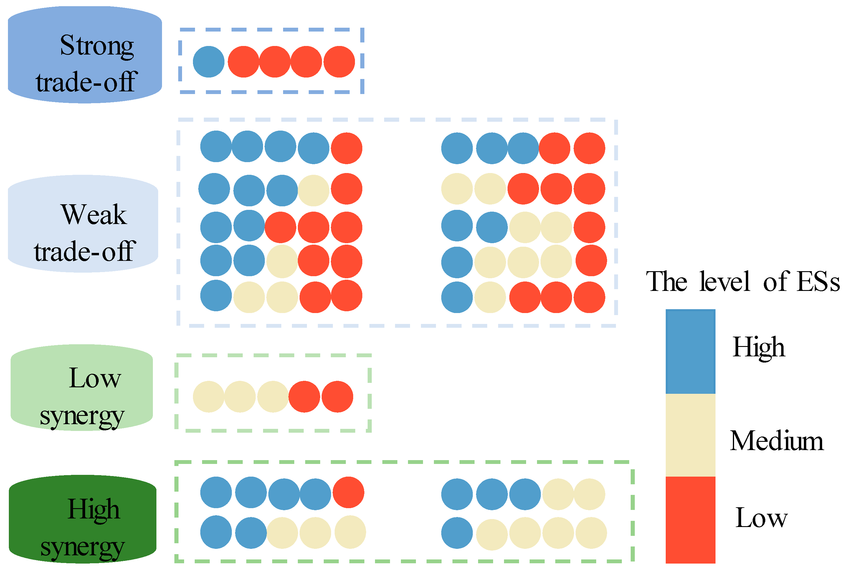
Develop trade-offs/synergy classification standards. The trade-offs are divided into strong trade-offs and weak trade-offs. As shown in Figure 3, a strong trade-off is a state where the service capacity is high and the others are low; a weak trade-off is a state where the capacities (classes) of service types 2, 3, or 4 are high and the other services are low. Synergy is divided into high synergy and low synergy. High synergy means that all five service capabilities are high, which is the most coordinated state and the ultimate goal of ecosystem management; low synergy means that all five service capabilities are low, and this state is the least ideal.

3. Results and Analysis

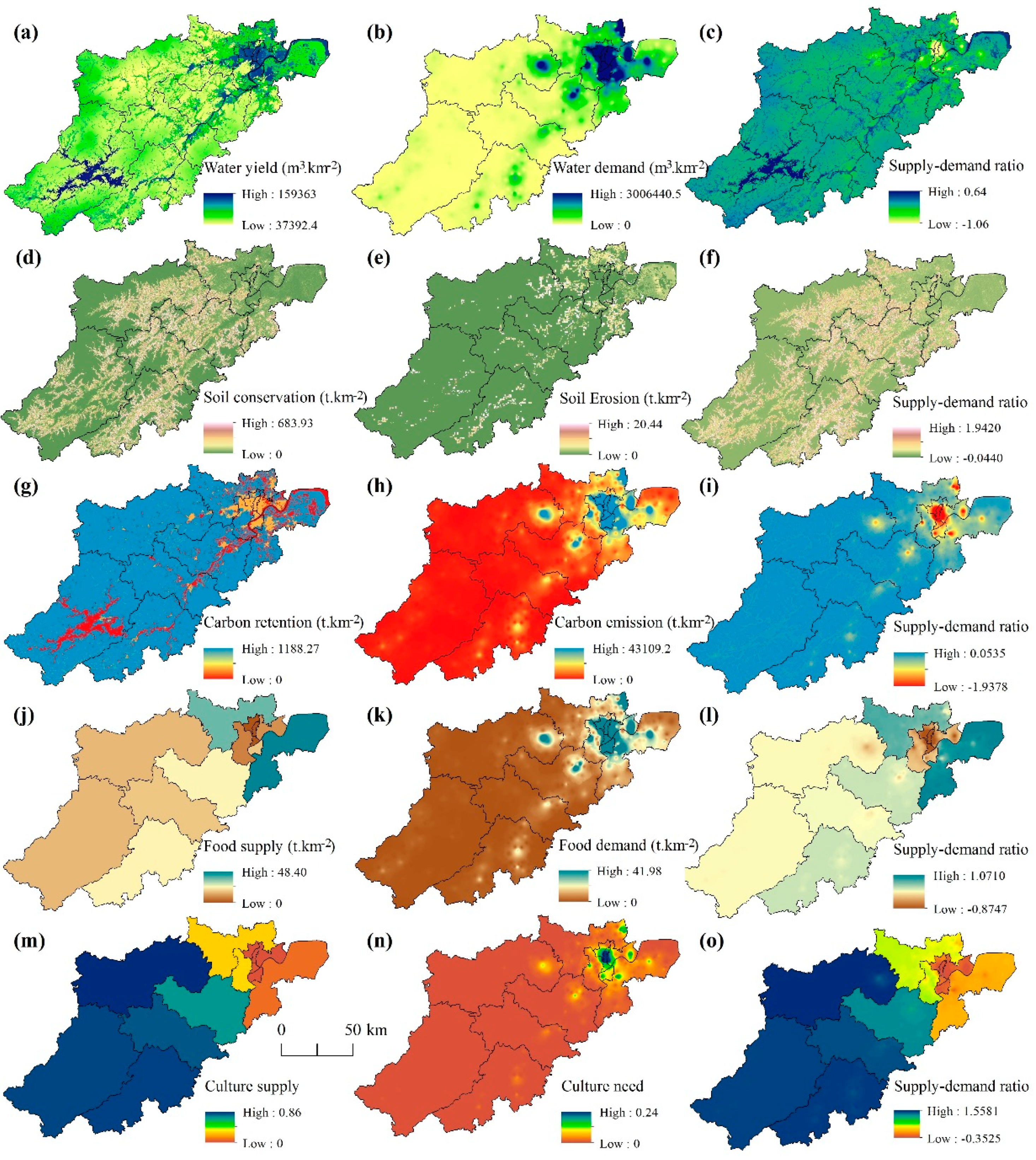
3.1. Spatial Characteristics of Ecosystem Service Supply and Demand

The water yield, soil conservation, food supply, and entertainment and leisure supply of Hangzhou’s ESs exceeded demand, whereas carbon retention supply services were less than demand (

Table 1. Status of supply and demand of ESs in Hangzhou.

Counties	Water Yield Services (m3·km−2)		Soil Conservation Services (t·km−2)		Carbon Retention Services (t·km−2)		Food Supply Services (t·km−2)		Leisure and Entertainment Services
	Supply	Demand	Supply	Demand	Supply	Demand	Supply	Demand	Supply	Demand
Shangcheng	116,546.33	95,501.74	10.59	0.37	302.55	18,430.29	0.009	17.946	0.146	0.104
Xiacheng	129,198.27	14,3870.95	16.02	0.05	190.31	30,662.13	0.004	29.856	0.058	0.172
Jianggan	113,478.94	8293.06	11.78	0.44	205.37	12,063.33	9.189	11.746	0.049	0.068
Gongshu	111,746.62	27,764.64	20.37	0.48	310.96	13,958.39	0.005	13.591	0.120	0.078
Xihu	84,199.26	2625.24	30.44	0.63	555.14	5747.85	6.865	5.597	0.367	0.032
Binjiang	117,642.01	25,410.19	8.74	0.56	244.91	12,858.50	16.452	12.520	0.078	0.072
Xiaoshan	83,535.33	385.14	20.54	0.78	399.24	4050.26	48.395	3.944	0.191	0.023
Yuhang	74,897.93	311.22	27.68	0.70	565.70	2772.74	36.566	2.700	0.350	0.016
Fuyang	62,906.02	87.93	50.41	0.40	886.23	1158.99	22.301	1.129	0.715	0.007
Lin’an	60,468.36	27.38	30.52	0.22	1038.57	620.06	14.401	0.604	0.855	0.003
Tonglu	61,657.02	27.90	37.19	0.17	983.21	370.78	16.530	0.361	0.801	0.002
Chun’an	70,967.40	4.43	25.11	0.09	962.67	141.77	14.486	0.138	0.818	0.001
Jiande	63,334.48	27.51	46.42	0.40	985.59	461.38	22.045	0.449	0.829	0.003
Hangzhou	68,721.60	1926.08	32.70	0.32	873.02	1396.64	20.727	1.331	0.701	0.008

, Figure 4). There were obvious spatial differences in the supply and demand of different types of ESs.

In terms of the function of water yield, the supply of Hangzhou’s annual water yield exceeded demand, with the total amount of water yield reaching 115.85 × 10⁸ m³ and the demand for water yield services reaching 32.47 × 10⁸ m³ in 2018. The high-value area of water yield per unit area was concentrated in the urban area of Hangzhou. The presence of developed land increased the surface impermeable area and had a strong ability to intercept precipitation, followed by the Qiandao Lake in the southwest. The main urban area of Hangzhou had the highest water demand per unit area, with a high regional population density, high urbanization levels and industrial agglomeration, etc., which displayed a great demand for water resources, whereas Chun’an and Jiande presented a low water demand, low population density, and a relatively low urbanization level. Soil conservation services were generally oversupplied, with a total supply of 5.51 × 10⁵ t.km⁻² and a soil conservation volume per unit area of 32.70 t·km⁻². The areas with a high average soil conservation volume were concentrated in areas with a slightly higher topographic relief. The vegetation coverage was relatively high and the soil was not easily eroded, as observed in the mountainous areas in Jiande and Chun’an. The total demand for soil conservation services was 5.37 × 10³ t·km⁻², and the soil conservation per unit area was 0.32 t·km⁻². The high-demand areas were concentrated in the northeast corner of Hangzhou, which was the estuary of Qiantang River.

The total supply of carbon retention services was 14.72 × 10⁶ t·km⁻² and the total demand was 23.54 × 10⁶ t·km⁻². The supply of carbon retention services was greatly affected by land use types, and the ecological land, such as forest and grassland, had a significant impact on regional carbon retention supply services. The high-demand area of carbon retention was concentrated in the main urban area of Hangzhou, with developed social economy and the huge consumption of oil, natural gas, and other energy resources. The total supply of the food service was 34.94 × 10⁴ t·km⁻²; the total demand was 1.69 × 10⁴ t·km⁻². The areas with high food supply were concentrated in Xiaoshan and Yuhang districts in the lower reaches of the Yangtze River. The soil is fertile and the arable land is vast. The food high-demand area was concentrated in urban areas with high population density. The supply of leisure and entertainment services exceeded the demand. Leisure and entertainment service reflected people’s demand for green space, whereas the high-demand area of leisure and entertainment service was concentrated in the urban area of Hangzhou, where the per capita urban green space area was relatively low.

3.2. Analysis of the Matching of the Supply and Demand of Ecosystem Services

The ecosystem service supply and demand ratio (ESDR) values of water yield, soil conservation, carbon retention, food supply, and leisure and entertainment services in Hangzhou were 0.236, 0.092, −0.022, 0.429, and 1.263, respectively, and the comprehensive ES supply and demand ratio (CESDR) was 0.399 (

Table 2. ESDR in each district and county of Hangzhou.

Districts and Counties	Water Yield	Soil Conservation	Carbon Retention	Food Supply	Leisure and Entertainment	Comprehensive Supply–Demand Ratio
Shangcheng	−0.106	0.029	−0.818	−0.397	0.077	−0.243
Xiacheng	−0.439	0.045	−1.376	−0.661	−0.209	−0.528
Jianggan	0.081	0.032	−0.535	−0.057	−0.034	−0.103
Gongshu	0.015	0.056	−0.616	−0.301	0.076	−0.154
Xihu	0.161	0.085	−0.234	0.028	0.609	0.130
Binjiang	0.073	0.023	−0.569	0.087	0.010	−0.075
Xiaoshan	0.211	0.056	−0.165	0.984	0.307	0.279
Yuhang	0.217	0.077	−0.100	0.749	0.609	0.310
Fuyang	0.219	0.142	−0.012	0.469	1.291	0.422
Lin’an	0.226	0.086	0.019	0.305	1.552	0.438
Tonglu	0.238	0.105	0.028	0.358	1.455	0.437
Chun’an	0.283	0.071	0.037	0.318	1.489	0.440
Jiande	0.242	0.131	0.024	0.478	1.506	0.476
Hangzhou	0.236	0.092	−0.022	0.429	1.263	0.399

). The results showed that the supply quantity of ESDR and CESDR in the study area was larger than the demand, except for the carbon retention service. Different counties/districts had differences in different ecosystem services. The most prominent manifestation was that the supply and demand in the urban area of Hangzhou was relatively small, whereas the supply and demand in Jiande, Chun’an, and Tonglu counties far from the urban area were relatively high. This indicates that the urban area had a huge demand for ESs, which was likely to cause an imbalance in ecosystem supply and demand.

In terms of water yield services, the ESDR in the Shangcheng and Xiacheng districts was less than 0, indicating that for each of these districts, its own production of water resources could not meet its own demand. In the study area (Figure 4), the low-value area was concentrated in the main urban areas, whereas the high-value area was centered on Qiandao Lake in Jiande city. The ESDRs of soil conservation services were all greater than zero, with Fuyang District (0.142) and Jiande City (0.131) as the high-value districts. It decreased from higher terrain to low-lying terrain. In terms of the carbon retention service, the ESDR of nine counties/districts was less than zero, and only four counties/districts had an ESDR greater than zero. The ESDR of the Shangcheng area of the municipal district (−1.376) was the lowest, indicating that the Shangcheng district produced a large amount of carbon emissions. In terms of spatial areas (Figure 3), the ESDR was low in the Shangcheng and Xiacheng districts, and it was difficult to achieve a balance between supply and demand in relation to carbon retention services. The ESDR of food supply was the largest in Xiaoshan (0.984) and Yuhang (0.749), followed by counties and districts in the southwest, whereas central urban areas were the lowest, such as Shangcheng district (−0.397), Xiacheng District (−0.661), Jianggan District (−0.057), and Gongshu District (−0.301). Some local areas within a specific county or district also presented a low ESDR centered in an urban area, with developed land as the main area, whereas values for farmland, water bodies, grassland, and other areas of food production land were small or absent, so the urban food production capacity was relatively weak. The ESDRs of leisure and entertainment showed the urban area to be a low-value area, which means it is difficult to meet the needs of regional cities and people for leisure and entertainment. The ESDRs in Fuyang District (1.291), Lin’an District (1.552), Tonglu County (1.455), Chun’an County (1.489), and Jiande City (1.506) were relatively high. In terms of spatial areas, the ESDRs in the urban area were relatively low, and the ESDRs in the southwestern counties/districts were relatively high, which was closely related to the distribution of regional green areas.

3.3. Tradeoffs between Ecosystem Services

The spatial overlay of the supply of five types of ESs in Hangzhou was obtained and statistically classified (

Table 3. Classification criteria and statistics of trade-offs and synergies among the five ES types.

Service Relationship	Proportion of Area (%)	Subclass	Proportion of Area (%)	Supply Capacity Mix *	Proportion of Area (%)	Samples **
Trade off	98.11	Strong trade-off	1.89	1H4L	1.89	11,311; 31,111
		Weak tradeoff	96.22	1H1M3L	0.08	12,311; 32,111; 21,131
				1H2M2L	7.91	21,231; 21,213; 23,211
				1H3M1L	6.87	21,232; 21,223; 22,213; 22,231
				2H1M2L	30.26	11,323; 21,313; 12,313; 31,132; 11,332; 31,123; 31,213; 12,331; 32,113; 32,131
				2H2M1L	7.36	12,323; 21,233; 12,332; 21,323; 23,213; 32,123; 32,132; 31,223; 23,231; 22,313; 32,213
				2H3L	28.58	11,313; 31,113; 31,131; 11,331; 33,111
				2M3L	0.36	21,211
				3H1M1L	5.12	13,323; 12,333; 13,332; 32,133; 33,123; 31,323; 33,132; 23,313; 32,313; 33,213; 32,331
				3H2L	8.26	11,333; 13,313; 31,133; 13,331; 33,113; 31,313; 31,331; 13,311; 33,131
				4H1L	1.4	13,333; 33,133; 33,313; 31,333
Synergy	1.89	High synergy	1.89	4M1H	0.96	22,223; 22,232
				2H3M	0.75	22,233; 22,323; 23,223; 23,232
				3H2M	0.18	23,233; 23,323; 32,223; 32,323; 33,223
				4H1M	0	33,323
		Low synergy	0	3M2L	0	22,211

* Summary of service capacity classes of the 5 ES types: water yield, soil conservation, carbon retention, food supply, and leisure and entertainment. ** The 5 digitals are capacity classes of ecosystem services: 1—low, 2—medium, and 3—high, corresponding to 5 ES types: water yield, soil conservation, carbon retention, food supply, and leisure and entertainment.

). The supply of ESs was dominated by a trade-off relationship, with an area accounting for 98.11%, indicating that water yield, soil conservation, carbon retention, food supply, and entertainment and leisure services in Hangzhou were in a trade-off relationship. In the trade-off relationship, the area of strong trade-offs was relatively small, accounting for only 1.89%. The types were 11,311 and 31,111, respectively, indicating the largest carbon supply and water production, which were larger than other supply types. The area of weak trade-offs was relatively wide, accounting for 96.22%, of which there were more instances of 2-high, 1-medium, and 2-low types, accounting for 30.26% of the regional area, mainly including “11,323, 21,313, 12,313, 31,132, 11,332, 31,123, 31,213, 12,331, 32,113, 32,131” types. In addition, the distribution area of 2-high and 3-low types was also larger, accounting for 28.58%, including “11,313, 31,113, 31,131, 11,331, 33,111” types. From the perspective of ES synergy, the area of synergy was small, accounting for only 1.89%. There were many types of high-synergy distribution, such as “4M1H, 2H3M, 3H2M, and 4H1M“ types, indicating that the regional ESs presented characteristics of mutual promotion. This was prominently manifested in the high supply service capacity of 2, 3, or 4 service types of ecosystems in the region, whereas other supply services were high. The area of low-coordinated supply service types was small, including only one type “3M2L”, such as “22,211”. Water yield, soil conservation, and carbon retention supply services were at a medium level, whereas food supply and leisure and entertainment services were at a low level.

There were only nine superposition types of ES demand in Hangzhou (Figure 5); the low synergy was the dominant type, covering an area of 16,244.60 km², accounting for 96.40% of the total area, indicating that there was a low level of coordination among various demand services in the ecosystem in Hangzhou. The main types of low synergy were “11,111, 12,111, and 21,222”. Various demand services were at a low level, but they were able to meet urban development through mutual promotion. The high-synergy type had a small area distribution (143.97 km²), but there were four types—“22,222, 23,222, 32,333, and 33,333”. The trade-off relationship area of demand services was small; the areas of strong trade-off and weak trade-off were 202.23 km² and 261.16 km², and their types were 13,111 and 31,333, respectively.

4. Discussion

4.1. Analyzing Mechanisms of the Spatial Difference in ES Supply and Demand

ES supply refers to the ability of an ecological environment to provide ecosystem products and services for the development of human society [25]. The ES supply of Hangzhou presents the characteristic that the main urban area exhibited lower values than those of the suburban area, which is closely related to the regional natural background, socio-economic development, and land use/land cover [50]. Based on the natural background and land use changes in the study area, we selected six indicators: forest land area, developed land area, DEM, slope, annual average precipitation, annual average temperature, and population density. We used the spatial analysis module in ArcGIS10.5 software to calculate correlations between different layers in order to analyze the mechanism behind spatial differences in ES supply (

Table 4. Correlations between ecosystem supply services and different indexes/driver factors.

Influencing Factors	Ecosystem Supply Services
	Water Yield	Soil Conservation	Carbon Retention	Food Supply Service	Leisure and Entertainment
Forest area	0.795 **	0.638 **	0.989 **	0.533 **	0.677 **
Developed land area	0.550 **	−0.840 **	−0.472	0.127	−0.376
DEM	0.474	−0.059	0.689 **	−0.481	0.647 **
Slope	0.204	0.944 **	0.116	0.006	0.039
Annual precipitation	−0.059	−0.164	0.367	−0.426	0.505 **
Annual average temperature	0.214	0.141	−0.426	0.422	−0.501 **
Population density	0.374	−0.062	−0.406	0.160	−0.603 **

Note: ** denotes statistical significance at p = 0.01.

).

Land use changes in Hangzhou have significantly affected the spatial heterogeneity of ES supply. The supply of ESs and forest area showed a significant positive correlation, and the correlation coefficients were all greater than 0.5. On the other hand, developed land associated with human activities was mostly negatively related to ESs supply. The results of our study were similar to those of Xu et al. [51]. As the largest land use area in Hangzhou, forest is mostly distributed in the central and western regions of higher elevation and slope, and has a strong ES supply function. Forest areas had significant correlations with water yield, soil conservation, carbon retention, food supply service, and leisure and entertainment, with correlation coefficients of 0.795, 0.638, 0.989, and 0.533, 0.677, respectively. Forest is an important type of ecological land, and areas with high forest coverage also show high ES functions. The developed land in the center of Hangzhou is dense, and is a low-value area in terms of ES supply. The developed land area is negatively correlated with soil conservation, carbon retention, and leisure and entertainment. Elevation and slope have significant effects on carbon retention and soil conservation services. The correlation coefficient between annual average temperature, annual precipitation, and ES supply is very small, and did not pass the test of statistical significance. Water and heat conditions should be important factors affecting ESs supply level, but the combination of water and heat conditions in Hangzhou area may be relatively good, thus exerting less of an impact on the regional ES supply. Population density was negatively correlated with leisure and entertainment. Most importantly, the spatial distribution of developed land and ecological land (forest, grassland, and water) in Hangzhou was different, which also led to the imbalance in ES supply in different counties/districts.

ES demand mainly reflects the consumption of natural ecosystems, and is the process of human access and utilization of natural resources [51]. The spatial distribution of ES demand in Hangzhou shows that the suburbs had lower values than those of the city center, which is opposite to the ESs supply characteristics. This is closely related to social and economic factors, such as population density, land development and utilization, and the economic development level.

4.2. Mechanisms Influencing ES Supply and Demand Contradictions

ESs play a vital role in the sustainable development of human society [31,50]. In previous studies, the high-supply areas of ESs were concentrated in mountainous areas, whereas the high-demand areas of ESs were concentrated in plain areas [52,53]. These results are similar to the results obtained in our study. Compared with mountainous areas, plain areas are densely populated and have a high level of urbanization, and the area of ecological land is small. Therefore, the demand for various ES types in urban areas is far greater than that in mountain areas. In terms of ES spatial matching, there is a spatial contradiction between the supply and demand of urban ESs, and most of the ESs in urban areas are in a state of shortage, which heavily depends on the ecological services outside the city, especially in some international metropolis or provincial capital cities [30,54], which is consistent with our research results.

Hangzhou City is composed of 13 counties/districts. Due to differences in the development history and development levels in the city, the spatial distribution characteristics of the supply and demand of ESs are also different. The low-value areas in terms of ESDR and CESDR in Hangzhou are concentrated in downtown areas, such as Shangcheng District, Xiacheng District, Jianggan District, and Gongshu District. The high demand and low supply of ESs in Hangzhou is also the most prominent contradiction between the supply and demand of ESs. Yuhang, Lin’an, Fuyang, Yuhang and Xiaoshan, as satellite cities of the center of Hangzhou, are responsible for alleviating the pressure from the population and environment in the center. For example, Xiaoshan and Yuhang Districts provide a sufficient food supply for the city center, and Xihu District provides leisure and entertainment services for the residents of the city center. The imbalance between the supply and demand of ESs in Hangzhou is similar to that of Shanghai and Nanjing [27,55]. The urban center has a high level of social and economic development, absorbing a large portion of the population, and the continuous expansion of developed land area, resulting in an increase in the demand for ESs and weakening the supply capacity. The peripheral area of the city is usually an area with high ES supply but low demand [27]. The spatial imbalance between the supply and demand of ESs would be worsened by the development of urbanization and industrialization.

In fact, the mismatch between the supply and demand of regional ESs is a common phenomenon in a certain period of time, which is the result of the interaction of regional natural background, socio-economic development, land use changes, and other factors [56]. The contradiction between supply and demand of ESs exists not only on the macro-scale of mainland, country, and urban agglomeration [57,58], but also on the micro-level of parks, communities, and villages [59]. Human activities exist in the natural environment and always have positive and negative effects on the ecological environment. Therefore, the question of how to adjust human activities to make them conform to the laws of natural development is particularly important. Many studies have revealed that human intervention activities (such as a harmonious land use and the application of government ecological protection policies) are conducive to improving and enhancing the supply functions of the ecosystem [22,50]. We need to deal with the relationship between urbanization, industrialization, and ecosystems; control the expansion rate of developed land; and plan land use rationally, so as to effectively alleviate the conflict between the supply and demand of ESs, and realize the coordinated development of the two.

4.3. Strengths and Limitations

The novelty of this study is that we quantitatively identified the spatial distribution characteristics of the supply and demand of Hangzhou’s ESs and revealed the fact that the demand for ESs in the central urban area exceeded the supply, and that the supply of ESs in Hangzhou was dominated by trade-offs. By analyzing the factors affecting the supply of ESs, governments should protect forests, increase ecological land, and reduce the expansion of developed land onto ecological protection lands.

The research on the supply and demand of ESs covers a wide range of areas. ESs involve ecology, economics, geography, and other disciplines. The structural and functional changes of ESs involve the regional natural background and the socio-economic development process [25,50]. All of these indicate that the research into ESs has a certain complexity, so it is difficult to systematically and comprehensively analyze all the functional types and processes of ES supply and demand. Therefore, this study also has the following limitations.

Our study only analyzed the spatial distribution characteristics of ESs in Hangzhou in 2018. We intend to carry out an analysis of the characteristics of the spatiotemporal changes of ESs in a long-term sequence. We considered the five main types of ESs in the study area, but in the context of rapid urbanization, human activities will affect multiple ES functions. In the future, we will increase our studies to include multiple ESs to more comprehensively reflect the changes in regional ecosystems. Although the InVEST model is currently widely used, it has certain limitations, as described in the software documentation [5]. Therefore, we need to further verify the modeling results to improve the accuracy of the ES assessments [29].

In addition, it is of great significance to explore the effect of regional natural environment, socio-economic, cultural development, and other factors on spatiotemporal changes and the spatial flow of ESs. Moreover, the spatial mismatch between ES supply and demand could easily lead to environmental equity problems [56], in which the central city transfers polluting industries to its suburbs and small cities and absorbs the resources, talents, and other elements of surrounding cities to enhance itself. This also involves geographic, economic, industrial, and other multidisciplinary knowledge, which is also worth exploring further.

5. Conclusions

Taking the Hangzhou region as a study area, in this study, we quantitatively evaluated the supply and demand of the five types of ESs, analyzed their spatial distribution and matching mechanisms, explored trade-off relationships between the supply and demand of five types of ESs. The main conclusions derived from the results of this analysis are summarized as follows.

The ESs of Water yield, soil conservation, food supply, and leisure and entertainment in Hangzhou exhibited an excess of supply, and carbon retention services were in short supply. There was an obvious spatial heterogeneity in the supply and demand of different types of ESs. With the exception of for carbon retention services, the ESDR and CESDR values of the other four types of ESs were greater than zero. The ES supply was dominated by trade-off relationships (98.11%), whereas the demand for services was dominated by low synergy (96.40%). The effect of each influencing factor on the supply of ESs was different, and the areas of forest and developed land showed a significant influence on regional ecosystem supply. In order to promote the coordinated development of ESs in Hangzhou, it is necessary to pay more attention to the protection of ecological land and appropriately control the expansion rate of developed land.

References

1. Costanza, R.; d’Arge, R.; De Groot, R.; Farber, S.; Grasso, M.; Hannon, B.; Limburg, K.; N aeem, S.; O’neill, R.V.; Paruelo, J. The value of the world’s ecosystem services and natural capital. Nature 1997, 387, 253–260. [Google Scholar] [CrossRef]
2. Reid, W.V.; Mooney, H.A.; Cropper, A.; Capistrano, D.; Carpenter, S.R.; Chopra, K.; Dasgupta, P.; Dietz, T.; Duraiappah, A.K.; Hassan, R.; et al. Ecosystems and Human Well-Being-Synthesis: A Report of the Millennium Ecosystem Assessment; Island Press: Washington, DC, USA, 2005. [Google Scholar]
3. Yee, S.H.; Paulukonis, E.; Simmons, C.; Russell, M.; Fulford, R.; Harwell, L.; Smith, L. Projecting effects of land use change on human well-being through changes in ecosystem services. Ecol. Model. 2021, 440, 109358. [Google Scholar] [CrossRef] [PubMed]
4. Crossman, N.D.; Burkhard, B.; Nedkov, S.; Willemen, L.; Petz, K.; Palomo, I.; Drakou, E.G.; Martín-Lopez, B.; McPhearson, T.; Boyanova, K. A blueprint for mapping and modelling ecosystem services. Ecosyst. Serv. 2013, 4, 4–14. [Google Scholar] [CrossRef]
5. Li, J.; Bai, Y.; Alatalo, J.M. Impacts of rural tourism-driven land use change on ecosystems services provision in Erhai Lake Basin, China. Ecosyst. Serv. 2020, 42, 101081. [Google Scholar] [CrossRef]
6. Tian, P.; Cao, L.; Li, J.; Pu, R.; Shi, X.; Wang, L.; Liu, R.; Xu, H.; Tong, C.; Zhou, Z. Landscape grain effect in Yancheng coastal wetland and its response to landscape changes. Int. J. Environ. Res. Public Health 2019, 16, 2225. [Google Scholar] [CrossRef] [Green Version]
7. Capriolo, A.; Boschetto, R.; Mascolo, R.; Balbi, S.; Villa, F. Biophysical and economic assessment of four ecosystem services for natural capital accounting in Italy. Ecosyst. Serv. 2020, 46, 101207. [Google Scholar] [CrossRef]
8. El Chami, D.; Daccache, A.; El Moujabber, M. What are the impacts of sugarcane production on ecosystem services and human well-being? A review. Ann. Agric. Sci. 2020, 65, 188–199. [Google Scholar] [CrossRef]
9. Liu, Y.; Liu, Y.; Li, J.; Sun, C.; Xu, W.; Zhao, B. Trajectory of coastal wetland vegetation in Xiangshan Bay, China, from image time series. Mar. Pollut. Bull. 2020, 160, 111697. [Google Scholar] [CrossRef]
10. Ahmadi, M.S.; Sušnik, J.; Veerbeek, W.; Zevenbergen, C. Towards a global day zero? Assessment of current and future water supply and demand in 12 rapidly developing megacities. Sustain. Cities Soc. 2020, 61, 102295. [Google Scholar] [CrossRef]
11. Knowlton, J.L.; Halvorsen, K.E.; Flaspohler, D.J.; Webster, C.R.; Abrams, J.; Almeida, S.M.; Arriaga-Weiss, S.L.; Barnett, B.; Cardoso, M.R.; Cerqueira, P.V. Birds and Bioenergy within the Americas: A Cross-National, Social–Ecological Study of Ecosystem Service Tradeoffs. Land 2021, 10, 258. [Google Scholar] [CrossRef]
12. Aziz, T. Changes in land use and ecosystem services values in Pakistan, 1950–2050. Environ. Dev. 2020, 37, 100576. [Google Scholar] [CrossRef]
13. Landuyt, D.; Broekx, S.; Goethals, P.L. Bayesian belief networks to analyse trade-offs among ecosystem services at the regional scale. Ecol. Indic. 2016, 71, 327–335. [Google Scholar] [CrossRef]
14. Costanza, R.; Daly, L.; Fioramonti, L.; Giovannini, E.; Kubiszewski, I.; Mortensen, L.F.; Pickett, K.E.; Ragnarsdottir, K.V.; De Vogli, R.; Wilkinson, R. Modelling and measuring sustainable wellbeing in connection with the UN Sustainable Development Goals. Ecol. Econ. 2016, 130, 350–355. [Google Scholar] [CrossRef]
15. Davies, Z.G.; Edmondson, J.L.; Heinemeyer, A.; Leake, J.R.; Gaston, K.J. Mapping an urban ecosystem service: Quantifying above-ground carbon storage at a city-wide scale. J. Appl. Ecol. 2011, 48, 1125–1134. [Google Scholar] [CrossRef] [Green Version]
16. Wu, C.; Chen, B.; Huang, X.; Wei, Y.D. Effect of land-use change and optimization on the ecosystem service values of Jiangsu province, China. Ecol. Indic. 2020, 117, 106507. [Google Scholar] [CrossRef]
17. Du, X.; Huang, Z. Ecological and environmental effects of land use change in rapid urbanization: The case of hangzhou, China. Ecol. Indic. 2017, 81, 243–251. [Google Scholar] [CrossRef]
18. Constant, N.L.; Taylor, P.J. Restoring the forest revives our culture: Ecosystem services and values for ecological restoration across the rural-urban nexus in South Africa. For. Policy Econ. 2020, 118, 102222. [Google Scholar] [CrossRef]
19. Larondelle, N.; Lauf, S. Balancing demand and supply of multiple urban ecosystem services on different spatial scales. Ecosyst. Serv. 2016, 22, 18–31. [Google Scholar] [CrossRef]
20. Wolff, S.; Schulp, C.; Verburg, P. Mapping ecosystem services demand: A review of current research and future perspectives. Ecol. Indic. 2015, 55, 159–171. [Google Scholar] [CrossRef]
21. Yu, C.; Cao, Y.; Li, G.; Tian, Y.; Fang, X.; Li, Y.; Tan, Y. Linking ecosystem services trade-offs, bundles and hotspot identification with cropland management in the coastal Hangzhou Bay area of China. Land Use Policy 2020, 97, 104689. [Google Scholar]
22. Sun, W.; Li, D.; Wang, X.; Li, R.; Li, K.; Xie, Y. Exploring the scale effects, trade-offs and driving forces of the mismatch of ecosystem services. Ecol. Indic. 2019, 103, 617–629. [Google Scholar] [CrossRef]
23. Kragt, M.E.; Robertson, M.J. Quantifying ecosystem services trade-offs from agricultural practices. Ecol. Econ. 2014, 102, 147–157. [Google Scholar] [CrossRef]
24. Wang, J.; Zhou, W.; Pickett, S.T.; Yu, W.; Li, W. A multiscale analysis of urbanization effects on ecosystem services supply in an urban megaregion. Sci. Total Environ. 2019, 662, 824–833. [Google Scholar] [CrossRef]
25. Burkhard, B.; Kroll, F.; Nedkov, S.; Müller, F. Mapping ecosystem service supply, demand and budgets. Ecol. Indic. 2012, 21, 17–29. [Google Scholar] [CrossRef]
26. Bryan, B.A.; Ye, Y.; Connor, J.D. Land-use change impacts on ecosystem services value: Incorporating the scarcity effects of supply and demand dynamics. Ecosyst. Serv. 2018, 32, 144–157. [Google Scholar] [CrossRef]
27. Shen, J.; Du, S.; Huang, Q.; Yin, J.; Zhang, M.; Wen, J.; Gao, J. Mapping the city-scale supply and demand of ecosystem flood regulation services—A case study in Shanghai. Ecol. Indic. 2019, 106, 105544. [Google Scholar] [CrossRef]
28. Castro, A.J.; Verburg, P.H.; Martín-López, B.; Garcia-Llorente, M.; Cabello, J.; Vaughn, C.C.; López, E. Ecosystem service trade-offs from supply to social demand: A landscape-scale spatial analysis. Landsc. Urban Plan. 2014, 132, 102–110. [Google Scholar] [CrossRef]
29. Benra, F.; Frutos, A.D.; Gaglio, M.; Lvarez-Garretón, C.; Felipe-Lucia, M.; Bonn, A. Mapping water ecosystem services: Evaluating InVEST model predictions in data scarce regions. Environ. Model. Softw. 2021, 138, 104982. [Google Scholar] [CrossRef]
30. González-García, A.; Palomo, I.; González, J.; López, C.; Montes, C. Quantifying spatial supply-demand mismatches in ecosystem services provides insights for land-use planning. Land Use Policy 2020, 94, 104493. [Google Scholar] [CrossRef]
31. Peng, J.; Wang, X.; Liu, Y.; Zhao, Y.; Xu, Z.; Zhao, M.; Qiu, S.; Wu, J. Urbanization impact on the supply-demand budget of ecosystem services: Decoupling analysis. Ecosyst. Serv. 2020, 44, 101139. [Google Scholar] [CrossRef]
32. Hasan, S.S.; Zhen, L.; Miah, M.G.; Ahamed, T.; Samie, A. Impact of land use change on ecosystem services: A review. Environ. Dev. 2020, 34, 100527. [Google Scholar] [CrossRef]
33. Lin, W.; Xu, D.; Guo, P.; Wang, D.; Li, L.; Gao, J. Exploring variations of ecosystem service value in Hangzhou Bay Wetland, Eastern China. Ecosyst. Serv. 2019, 37, 100944. [Google Scholar] [CrossRef]
34. Wang, C.; Yu, C.; Chen, T.; Feng, Z.; Wu, K. Can the establishment of ecological security patterns improve ecological protection? An example of Nanchang, China. Sci. Total Environ. 2020, 740, 140051. [Google Scholar] [CrossRef]
35. Zhang, J.; Zhu, W.; Zhu, L.; Li, Y. Multi-scale analysis of trade-off/synergy effects of forest ecosystem services in the Funiu Mountain Region. Acta Geogr. Sin. 2020, 75, 975–988. [Google Scholar]
36. Nachtergaele, F.; Velthuizen, H.; Verelst, L.; Wiberg, D. Harmonized World Soil Database (HWSD); Food Agriculture Organization of the United Nations: Rome, Italy, 2009. [Google Scholar]
37. China Economic and Social Big Data Research Platform. 2018. Available online: https://data.cnki.net (accessed on 15 March 2021).
38. Redhead, J.; Stratford, C.; Sharps, K.; Jones, L.; Ziv, G.; Clarke, D.; Oliver, T.; Bullock, J. Empirical validation of the InVEST water yield ecosystem service model at a national scale. Sci. Total Environ. 2016, 569, 1418–1426. [Google Scholar] [CrossRef] [PubMed] [Green Version]
39. He, S.; Su, Y.; Shahtahmassebi, A.R.; Huang, L.; Zhou, M.; Gan, M.; Deng, J.; Zhao, G.; Wang, K. Assessing and mapping cultural ecosystem services supply, demand and flow of farmlands in the Hangzhou metropolitan area, China. Sci. Total Environ. 2019, 692, 756–768. [Google Scholar] [CrossRef] [PubMed]
40. Hangzhou Water Resources Bulletin. 2018. Available online: http://ls.hangzhou.gov.cn (accessed on 15 March 2021).
41. Liu, C.; Wang, W.; Liu, L.; Li, P. Supply-demand matching of county ecosystem services in Northwest China: A case study of Gulang county. J. Nat. Resour. 2020, 35, 2177–2190. [Google Scholar]
42. Babbar, D.; Areendran, G.; Sahana, M.; Sarma, K.; Raj, K.; Sivadas, A. Assessment and prediction of carbon sequestration using Markov chain and InVEST model in Sariska Tiger Reserve, India. J. Clean. Prod. 2021, 278, 123333. [Google Scholar] [CrossRef]
43. Li, Z.; Ren, L.; Ma, R.; Liu, Y.; Yao, D. Temporal and spatial patterns and influencing factors of land use carbon emission at county level in Hangzhou city. Sci. Technol. Manag. 2020, 22, 1–9. [Google Scholar]
44. Eggleston, S.; Buendia, L.; Miwa, K.; Ngara, T.; Tanabe, K. (Eds.) Guidelines for National Greenhouse Gas Inventories. Volume 4: Agriculture, Forestry and Other Land Use; IPCC: Geneva, Switzerland, 2006; pp. 9–12. [Google Scholar]
45. Liu, L.; Liu, C.; Wang, C.; Li, P. Supply and demand matching of ecosystem services in loess hilly region: A case study of Lanzhou. Prog. Chem. 2019, 74, 1921. [Google Scholar]
46. Grossmann, M. Impacts of boating trip limitations on the recreational value of the Spreewald wetland: A pooled revealed/contingent behaviour application of the travel cost method. J. Environ. Plan. Manag. 2011, 54, 211–226. [Google Scholar] [CrossRef]
47. Simões, P.; Barata, E.; Cruz, L. Using Count Data and Ordered Models in National Forest Recreation Demand Analysis. Environ. Manag. 2013, 52, 1249–1261. [Google Scholar] [CrossRef] [PubMed]
48. Yang, M.; Zhang, Y.; Wang, C. Spatial-temporal Variations in the Supply-demand Balance of Key Ecosystem Services in Hubei Province. Resour. Environ. Yangtze Basin 2019, 28, 2080–2091. [Google Scholar]
49. Shi, Y.; Shi, D.; Zhou, L.; Fang, R. Identification of ecosystem services supply and demand areas and simulation of ecosystem service flows in Shanghai. Ecol. Indic. 2020, 115, 106418. [Google Scholar] [CrossRef]
50. Costanza, R.; De Groot, R.; Braat, L.; Kubiszewski, I.; Fioramonti, L.; Sutton, P.; Farber, S.; Grasso, M. Twenty years of ecosystem services: How far have we come and how far do we still need to go? Ecosyst. Serv. 2017, 28, 1–16. [Google Scholar] [CrossRef]
51. Xu, Q.; Yang, R.; Zhuang, D.; Lu, Z. Spatial gradient differences of ecosystem services supply and demand in the Pearl River Delta region. J. Clean. Prod. 2021, 279, 123849. [Google Scholar] [CrossRef]
52. Qingchun, G.; Jinmin, H.; Guoping, R.; Mu, L.; Aiqi, C.; Wenkai, D.; Hong, C. Ecological indexes for the analysis of the spatial-temporal characteristics of ecosystem service supply and demand: A case study of the major grain-producing regions in Quzhou, China. Ecol. Indic. 2020, 108, 105748. [Google Scholar]
53. Cao, T.; Yi, Y.; Liu, H.; Xu, Q.; Yang, Z. The relationship between ecosystem service supply and demand in plain areas undergoing urbanization: A case study of China’s Baiyangdian Basin. J. Environ. Manag. 2021, 289, 112492. [Google Scholar] [CrossRef]
54. Chen, J.; Jiang, B.; Bai, Y.; Xu, X.; Alatalo, J.M. Quantifying ecosystem services supply and demand shortfalls and mismatches for management optimisation. Sci. Total Environ. 2019, 650, 1426–1439. [Google Scholar] [CrossRef]
55. Tao, Y.; Wang, H.; Ou, W.; Guo, J. A land-cover-based approach to assessing ecosystem services supply and demand dynamics in the rapidly urbanizing Yangtze River Delta region. Land Use Policy 2018, 72, 250–258. [Google Scholar] [CrossRef]
56. Zhai, T.; Wang, J.; Jin, Z.; Qi, Y.; Fang, Y.; Liu, J. Did improvements of ecosystem services supply-demand imbalance change environmental spatial injustices? Ecol. Indic. 2020, 111, 106068. [Google Scholar] [CrossRef]
57. Schulp, C.J.; Lautenbach, S.; Verburg, P.H. Quantifying and mapping ecosystem services: Demand and supply of pollination in the European Union. Ecol. Indic. 2014, 36, 131–141. [Google Scholar] [CrossRef]
58. Baró, F.; Haase, D.; Gómez-Baggethun, E.; Frantzeskaki, N. Mismatches between ecosystem services supply and demand in urban areas: A quantitative assessment in five European cities. Ecol. Indic. 2015, 55, 146–158. [Google Scholar] [CrossRef] [Green Version]
59. Bae, J.; Ryu, Y. Land use and land cover changes explain spatial and temporal variations of the soil organic carbon stocks in a constructed urban park. Landsc. Urban Plan. 2015, 136, 57–67. [Google Scholar] [CrossRef]
Figure 1. The study area, Hangzhou. Notes: (a) Lin’an, (b) Fuyang, (c) Tonglu, (d) Chuan’an, (e) Jiande. The main urban area of Hangzhou includes Shangcheng District, Xiacheng District, Xihu District, Gongshu District, Jianggan District, Xiaoshan District, and Yuhang District.
Land 10 00582 g001
Figure 2. Percentage of energy consumption carbon emissions in Hangzhou.
Land 10 00582 g002
Figure 3. Schematic diagram of ES trade-offs/synergy analysis. Each circle represents a type of ecosystem service. The circle has no fixed position and can be changed in order. Considering that there are many types of overlay, only the five types of ecosystem services appearing in this article are listed. The order of the circles in different colors reflects the superposition of different levels of ecosystem service types.
Land 10 00582 g003
Figure 4. Spatial distribution of supply and demand of various ESs in Hangzhou. (a,d,g,j,m) respectively represent the ES supply of water yield, soil conservation, carbon retention, food supply, and Leisure and Entertainment. (b,e,h,k,n) respectively represent the ES demand of water yield, soil conservation, carbon retention, food supply, and Leisure and Entertainment. (c,f,i,l,o) respectively represent the ES supply-demand ratio of water yield, soil conservation, carbon retention, food supply, and Leisure and Entertainment.
Land 10 00582 g004
Figure 5. Ecosystem demand service overlay relationships.
Land 10 00582 g005