Large-Scale Soil Erosion Estimation Considering Vegetation Growth Cycle

Abstract

The Revised Universal Soil Loss Equation (RUSLE) was used to predict the potential soil erosion; it simply multiplies rainfall erosivity and land cover management factors; it does not consider the dynamics of these two factors during a given year or the effect of vegetation growth cycle on soil erosion estimates. This study developed a new method that considers the vegetation growth cycle in different periods of the year by matching monthly rainfall erosivity and a management factor using the entire surface of China as the study area. The data were input into the original equation, and the two methods to estimate soil erosion were compared. Finally, patterns and mechanisms of the influence of vegetation growth cycle on RUSLE estimations under different climatic conditions were obtained. The results show that vegetation coverage inhibits the effect of rainfall on soil erosion potential, which is related to the average and coefficient of variation of cover-management factor and the average of rainfall erosivity due to the significant variations in weather patterns in winter and summer in China. This article discusses the influence of the vegetation growth cycle on the estimation of large-scale soil erosion, which is a key to having a better estimation.

1. Introduction

Soil resources play an important role in maintaining the ecological system of the Earth surface. However, nearly 2 billion hectares of land, approximately 15% of the Earth’s surface, suffer from soil degradation, with over half of soil erosion caused by water-related disasters [1]. Erosion directly affects food and water security, compromises agricultural productivity, and contaminates sources of water [2,3]. China is one of the countries that experiences the most severe soil erosion in the world, where 50.78% of the surface area, over 4.8253 million km², has undergone moderate soil erosion [4]. The primary and most profound problem with soil erosion is the loss of soil, which can lead to land degradation, loss of arable land, and in some cases even desertification [5,6]. Consequently, an accurate estimation of soil erosion at large scales is highly important for land use planning and sustainable development policies.

In the 1950s, the demand for a simple method to estimate annual average soil loss induced by rainfall in the United States led to the development of soil erosion models such as the Universal Soil Loss Equation (USLE) [7] and the revised version of the USLE (RUSLE) [8]. The RUSLE has since become one of the most widely used soil erosion prediction models in the world [9], with most studies conducted in the sub-Saharan region [10,11] or watersheds and seldom applied on a large scale [12]. As a complex geographical phenomenon [13], the mechanisms of soil erosion change with the spatial scale [14,15]. Xu [16] studied the spatial-temporal effects of soil erosion on a large scale and showed that the geographical environment becomes more complex with the increase in the scale. Moreover, the random combination of different geographical factors determines soil erosion as a typical nonlinear distribution parameter system, and on a larger spatial scale, the characteristics become stronger. Therefore, when it comes to estimating soil erosion on a large scale, the methods that do not consider the processes of soil erosion or the important variables with high annual variations such as rainfall are no longer applicable [17]. Therefore, new methods considering the spatiotemporal variability of each element in the RUSLE equation are required [18,19].

Annual soil loss is estimated from the combination of five factors contained in the RUSLE: rainfall-runoff erosivity (R-factor), soil erodibility (K-factor), slope length and slope steepness (LS-factor), cover and management (C-factor), and support practice (P-factor). Among these, the K-factor always displays an intermediate state in a year because it changes in the multiyear scale [20]. The LS-factor and P-factor are always in a relatively static state when there are no natural changes such as landslides or man-made changes and new protective measures [21]. The R-factor is calculated using the multi-annual average of the total storm erosivity index [22], while annual rainfall erosivity is characterised by seasonal variations, similar to the C-factor [23]. Changes in the C-factor are correlated with precipitation, which is the leading cause of the R-factor, while the wave of the R-factor can carry weight with the natural changes in plant growth, which is the main component of the C-factor [8]. As a result, one possible way to improve soil erosion prediction is to establish a relationship between the R-factor and C-factor.

Many researchers have reported the spatiotemporal variability of rainfall erosivity and the time-series C factor, which are closely related to the R-factor and C-factor in this paper, with the first one meaning multiyear rainfall erosivity index and the latter representing soil use and management. Xihua Yang [24] discussed the variations in the C-factor over 13 years using a correlation model with a resolution of 500 m to study soil erosion in New South Wales, Australia. Angulo-Martínez and Beguería [25] used daily rainfall records to calculate the R-factor at a high time resolution of at least 15 min, with other similar studies on seasonal [17] or monthly scale [26]. However, most of these studies optimised a single factor instead of considering the association of the R-factor with the C-factor. Studies that considered the seasonal variations in the R-factor and C-factor simultaneously also have some drawbacks. For example, Wang, et al. [27] found that changing the rainfall amount directly affects the value of the normalised difference vegetation index (NDVI), but they did not connect this discovery to the calculation of the RUSLE equation. Durigon, et al. [28] merely compared satellite images to seek out the effect of seasonal rainfall on the C-factor the following year, without considering the interaction between rainfall erosivity and vegetation cover.

The same R can result in different effects on soil erosion according to the time of the year, and depending on different factors, such as crop cover which changes seasonally. High R can occur under excellent crop conditions or residue cover that does not affect soil erosion processes. On the contrary, if a bare soil period matches a sporadic high rainfall erosivity event, extreme soil erosion will occur [29,30]. With this in mind, this study aims to evaluate the seasonal variations of R and C to discuss the uncertainties in soil erosion estimation results. The calculation was carried out by matching C and R on a monthly scale based on the RUSLE using data from China such as rainfall, NDVI, and land use from 2018. Finally, the new results were compared with those calculated using the original RUSLE to cast new light on the spatial distribution of soil loss in China.

2. Data and Methods

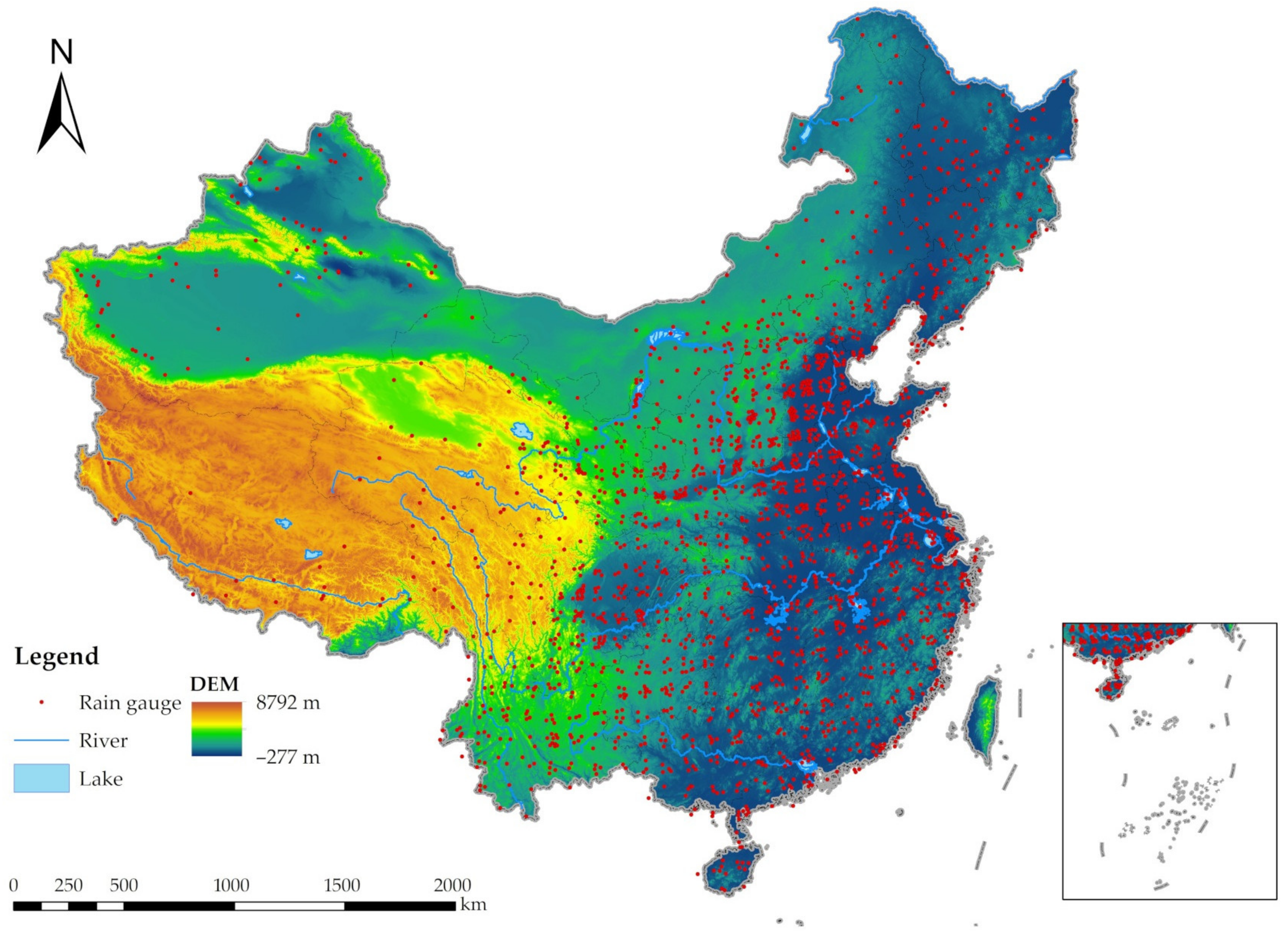
2.1. Data and Study Area

The entire surface of China was used as the study areas, from 3°51′ to 53°33′ N, and from 73°33′ to 135°05′ E. The altitude change in China is as high as 8999.43 m (highest elevation at Qomolangma, is 8844.43 m above the sea level; lowest elevation in Turpan Basin is 155 m below the sea level). The climate types in China are diverse with significant spatial differences. The R-factor and C-factor in RUSLE are sensitive to climate variations; therefore, in this, the study area was divided into regions according to climate types. The Köppen climate classification uses the monthly average temperature and precipitation as the classification index [31], which is consistent with the objective of this study and has strict standards, clear boundaries, and convenient applications. Therefore, this study uses this classification for dividing the study area into different regions to investigate the uncertainties in soil erosion estimates calculated by RUSLE.

The data used in this study are listed in

Table 1. Data source and resolution of each factor.

Data	Source	Time	Resolution	Calculation Purpose
Rainfall	Hourly data for rain gauges at 2168 stations	2018	T: hour S: 10 km	R-factor
Vegetation coverage	Terra satellite MODIS sensor data MODIS_DATA	2018	T: month S: 1 km	C-factor
Elevation	China DEM Data		T: annual average S: 10 km	LS-factor
Soil	Global Soil Database		T: annual average S: 10 km	K-factor
Land use	Land cover based on ESA Envisa satellite MERIS sensor data		T: annual average S: 10 km	P-factor

Note: T and S represent the time and spatial resolution, respectively.

.

2.2. Soil Erosion Estimation Model Considering Vegetation Growth Cycle

Soil erosion is calculated by using the following multiplicative equation [8,32]:

$$A_a=R_a·C_a·LS·K·P$$

(1)

where A_a (Mg ha⁻¹ yr⁻¹) is the soil erosion in a year per unit area, R_a (MJ mm h⁻¹ ha⁻¹ yr⁻¹) is the annual cumulative rainfall erosivity, C_a is an annual variable representing land cover and management condition, L is the slope length factor, S is the slope steepness factor, K (Mg h MJ⁻¹ mm⁻¹) is the soil erodibility factor, P is the soil conservation or prevention practices factor, and L, S, C_a, and P are all dimensionless values.

R_a is the main dynamic factor in the model, reflecting the potential soil erosion caused by rainfall. After screening the rainfall events from the original data, we can obtain the erosive rainfall events, and R_a is calculated using the method proposed by [33]:

$$R_a={\displaystyle \sum }_{j=1}^m{\displaystyle \sum }_{k=1}^{mj}\left(E{I}_{30}\right)k$$

(2)

where EI₃₀ is the rainfall runoff erosivity of a single k event, m is the number of observed years, and mj is the erosive event of a given year j. The EI₃₀ algorithm is expressed as follows:

$$E{I}_{30}=E·I_{30}$$

(3)

where E is the total rainfall energy in a rainfall event, and I₃₀ indicates the maximum 30-min rainfall intensity of the rainfall event. After screening the rainfall events, the energy E was calculated using the following formula:

$$E={{\displaystyle \sum }}_{r=1}^n\left(e_r·P_r\right)$$

(4)

where e_r and P_r are the unit rainfall kinetic energy (MJ hm⁻² mm⁻¹) and rainfall amount (mm) of the rainfall event r, and the formula for e_r is as follows:

$$e_r=0.29{\left[1-0.72exp\left(-0.082i_r\right)\right]}_{ }$$

(5)

where i_r is the rainfall intensity at the time of r (mm h⁻¹).

The maximum 30-min intensity of the rainfall event was calculated using the following formula:

$$I_{30}=P_{60}/1.0hr$$

(6)

where P₆₀ is the 60-min rainfall data at equal intervals.

In a rainfall erosion event, we use 60-min precipitation data at equal intervals to obtain EI₃₀. By using the following formula, the 60-min rainfall data can be successfully used to estimate rainfall erosivity where no finer time resolution data are available [34].

$${\left(E{I}_{30}\right)}_{bp}=1.730{\left(E{I}_{30}\right)}_{60}$$

(7)

Thus, the monthly rainfall erosivity R_m (MJ mm ha⁻¹ h⁻¹ mo⁻¹) can be calculated as the summation of EI₃₀ of the energy of all rainfall-induced erosion events in a month and the maximum rainfall intensity of the corresponding event for 30 min, and the annual erosivity factor R_a is the sum of the R_m values.

$$R_m={{\displaystyle \sum }}_{n=1}^{N}E{I}_{30}$$

(8)

$$R_a={{\displaystyle \sum }}_{m=1}^M{R}_m$$

(9)

where N is the total number of rainfall events in a month, and M the number of months in a year.

In this study, hourly rainfall data from 2168 rain gauges distributed across China for the year 2018 were used (Figure 1). Using MATLAB, R_a was calculated for each erosive rainfall event. The dispersion results were obtained by summing the monthly rainfall erosivity values. The ordinary kriging method was used for spatial interpolation, where the Box–Cox transformation method, which is a generalised power transformation method proposed by Box and Cox (1964), was employed for the normal transformation of the calculated R_a. The parameter of the kriging interpolation was set to 0.33, and the spatial resolution was set to 10 km.

C_a is the ratio of soil loss under actual vegetation and management conditions to the soil loss in bare continuous recreational land [35]. After obtaining the corresponding vegetation coverage data, NDVI is converted to vegetation coverage using the algorithm of Qi, et al. [36], and the results are calculated by referring to the method of [37].

$$fc=\frac{NDVI-NDV{I}_{min}}{NDV{I}_{max}-NDV{I}_{min}}$$

(10)

where fc is the vegetation coverage, NDVI_max and NDVI_min are the maximum and minimum NDVI of the research area, respectively. Then, the fc reference method is converted to C_m as follows:

$$C_m=\left\{\begin{array}{c}1,fc=0\\ 0.6508-0.3436\lg \left(fc\right),0<fc\le 78.3\%\\ 0,fc>78.3\%\end{array}\right.$$

(11)

Finally, the annual value of C_a, is obtained using the C_m values.

LS reflects the impact of topography. In this study, the calculation method of the slope length factor proposed by McCool, et al. [38] and Liu, et al. [39] was used. K refers to the sensitivity of the soil to denudation and transport of erosive media. This study uses the method proposed by Williams, et al. [40] which calculates Wd (sand%), Wi (silt%), Wt (clay%), and Wc (organic carbon %) to estimate the value of K. P is the ratio of soil loss to slope land cultivation after special management measures are taken. It is the inhibiting factor of erosion dynamics and plays the role of soil and water conservation. The calculation of P in this study was based on the use of previous research results, and the land types are divided into 11 categories, among which the p value of woodland, wetland, and bare land is 1, and the value of urban land and water bodies is 0 [41,42].

The RUSLE was used to calculate the average annual soil erosion. All factors reflect the annual average values but cannot reflect the changes within the year. Therefore, the traditional RUSLE fails to estimate the influence of seasonal variations on soil erosion. Since the monsoon climate affects most parts of China and the uneven distribution of precipitation in these regions leads to increased vegetation growth, the rainfall erosivity and land cover and management conditions in monsoon regions are greatly affected by seasonal changes. While the changes in topography, soil type, and land use type are negligible during the year, this study focuses on the calculation of R and C. Because of the fact that rainfall erosion is based on monthly accumulation, annual average soil erosion can be calculated by multiplying the corresponding value of land cover and management by monthly rainfall erosion and then by LS, K, and P. The formula for this calculation (RUSLE-dynaRC) is expressed as follows:

$$A_{dynaRC}={\displaystyle \sum }_{i=1}^N\left(R_i·C_i\right)·LS·K·P$$

(12)

where N = 12 representing the months of the year, R_i is the rainfall erosivity of the ith month, and C_i is the land cover and management in the ith month.

2.3. Uncertainty Analysis of Soil Erosion

To quantitatively demonstrate the annual and monthly values of R and C, and to consider the differences between the traditional RUSLE model and the method used in this study, it is necessary to calculate the dispersion of R and C within the year. The higher the dispersion, the greater the error in the original average. The degree of dispersion of R and C can be calculated using the coefficient of variation (CV), which is the ratio of the standard deviation of the original data to the average of the original data.

$${\mathrm{CV}}_R=\sqrt{\frac{1}{N}{\displaystyle \sum _{i=1}^N{\left(\frac{R_i}{\overline{R}}-1\right)}^2}}$$

(13)

$${\mathrm{CV}}_C=\sqrt{\frac{1}{N}{\displaystyle \sum _{i=1}^N{\left(\frac{C_i}{\overline{C}}-1\right)}^2}}$$

(14)

where $\overline{R}$ is the average annual rainfall-runoff erosivity factor, and $\overline{C}$ is the average annual land cover and management factor.

To describe the differences between the amount of soil erosion calculated by using the traditional RUSLE model and that calculated in this study, we define the uncertainty by using the following two indices: (1) The uncertainty event difference index (U_EDI), which reveals the distribution and degree of uncertainty but it is influenced by the original value and extreme values, and (2) U_NLI, which is a dimensionless factor used to change the absolute value of a numerical value to a relative value and reduce the influence of extreme values. Although the distribution of uncertainty cannot be displayed intuitively after mapping, this index is more reliable and easier to manage the outliers. The two methods can be expressed as follows:

$$U_{EDI\_ij}={\displaystyle \sum }_{i=1}^n{\displaystyle \sum }_{j=1}^m\left[A_{R\_ij}\left(t\right)-A_{dynaRC\_ij}\left(t\right)\right]$$

(15)

$$U_{NLI\_ij}={\displaystyle \sum }_{i=1}^n{\displaystyle \sum }_{j=1}^m\frac{A_{R\_ij}\left(t\right)-A_{dynaRC\_ij}\left(t\right)}{A_{R\_ij}\left(t\right)+A_{dynaRC\_ij}\left(t\right)}$$

(16)

where A_{R_ij} (Mg ha⁻¹ yr⁻¹) represents the amount of soil erosion calculated by using the traditional method on the grid of row i and column j at time t. A_{dynaRC_ij} (Mg ha⁻¹ yr⁻¹) represents the amount of soil erosion calculated using R and C matched monthly on the grid of row i and column j at time t.

3. Results

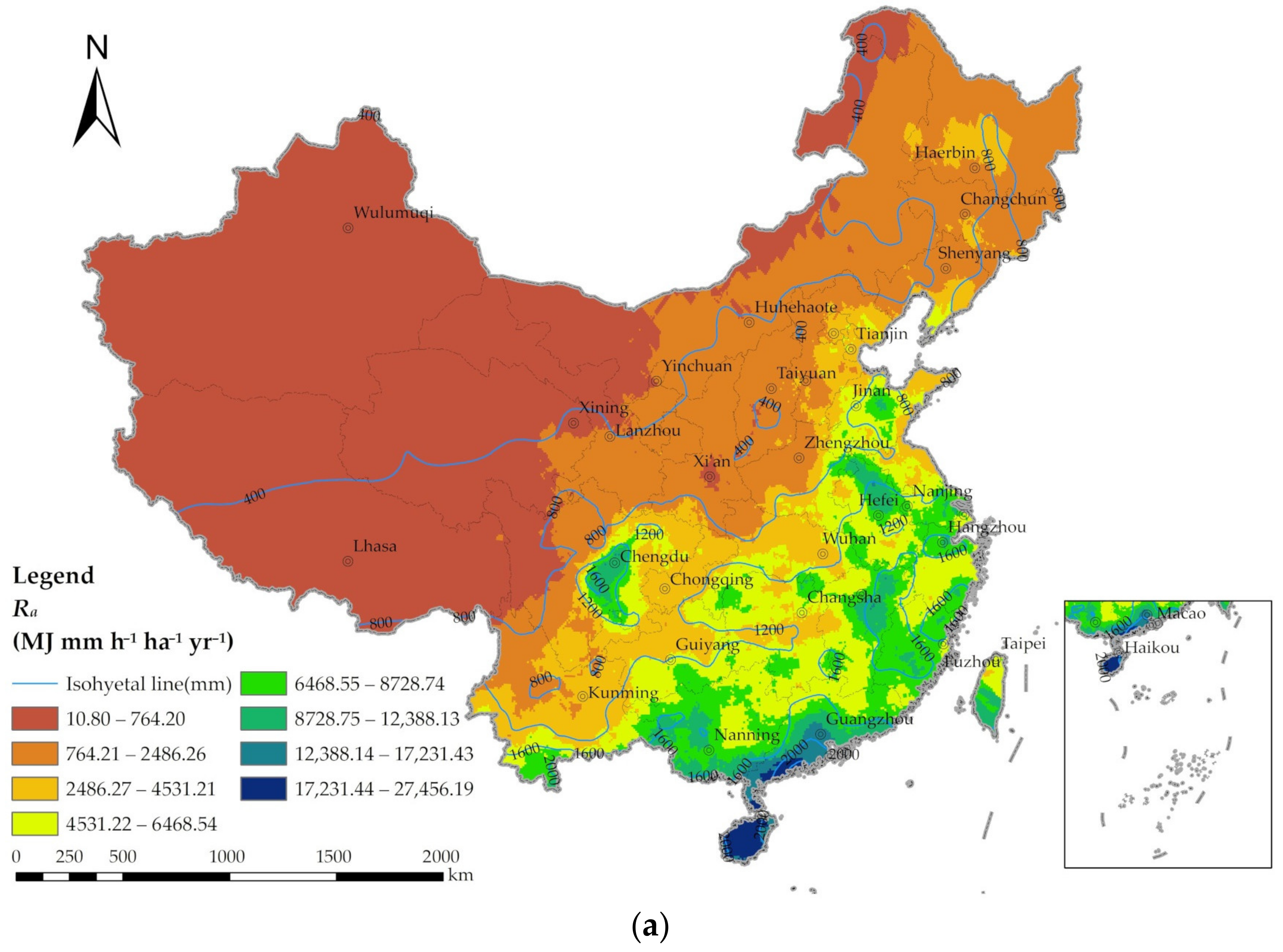
3.1. Calculation of R_a and C_a

Figure 2a shows the annual accumulation of R_a, with the minimum value of 10.79 MJ mm h⁻¹ ha⁻¹ yr⁻¹, the maximum of 27,456.19 MJ mm h⁻¹ ha⁻¹ yr⁻¹, and the average of 2058.34 MJ mm h⁻¹ ha⁻¹ yr⁻¹. Note that higher values of the rainfall erosion factor represent greater impacts on local soil erosion. Overall, the conditions vary between regions. Rainfall erosivity decreases from southeast to northwest, which almost coincides with the equal precipitation gradient in China. Rainfall erosion values are higher in coastal areas than in inland regions, and higher in the south than in the north. The highest value is observed in the southern tip of China, while the lowest value appears in the west. In the inclined banded area, the rainfall erosivity values are similar, while those in Harbin, Beijing, Tianjin, Chengdu, and other areas are low.

The C_a value was obtained using the NDVI data with a resolution of 10 km and one month, in China, in 2018, by mask extraction. The C_a value ranges between 0 and 1 and is dimensionless. Figure 2b shows that average C_a is 0.69. The lower the C_a value, the better the local vegetation conditions, and denser vegetation. In general, the vegetation cover increases from southeast to northwest in China, which almost coincides with the equal precipitation line. In southern China, the values in Wuhan, Nanjing, and Guangzhou are large. Nationwide, the lowest value appears in the south-eastern coastal region, and the highest value appears in the northwest. The effects of R_a and C_a on the U_NLI are discussed in Section 4.

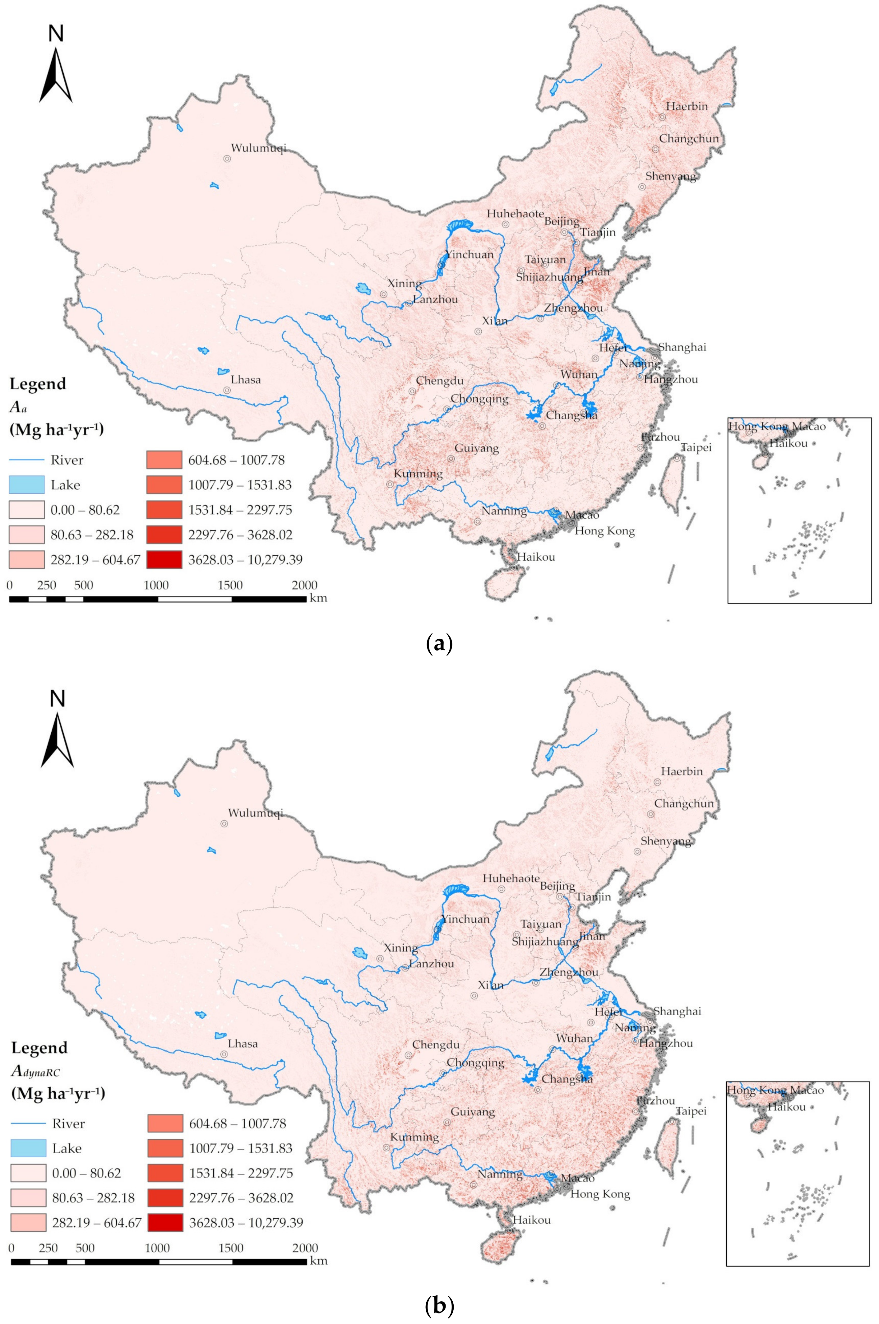
3.2. Nationwide Soil Erosion

After R_a and C_a were obtained, we matched the monthly R and C values to the amount of soil erosion in China through the traditional RUSLE and RUSLE-dynaRC. China was divided into 11 regions by climate type based on the Köppen climate classification, and the changes in R and C were obtained in each region on a monthly basis. Through the analysis of the absolute difference of R and C, the influence of two variables on the uncertainties in the soil erosion estimations was explored.

Figure 3 displays the distribution of soil erosion across China in 2018. The A_a value in Figure 3a was calculated using the RUSLE. The minimum value is 0, the maximum is 10,279.39 Mg ha⁻¹ yr⁻¹, and the average is 81.75 Mg ha⁻¹ yr⁻¹. In the A_a calculation, monthly matching was not considered. Instead, the annual cumulative values of R_a and C_a were directly multiplied, with L, S, Ca, P-factors to obtain the results. Overall, soil erosion extends from northeast to southwest. Note that soil erosion values are significantly higher around Beijing, Tianjin, and Jinan in the north, whereas they are significantly lower around Chengdu in the Sichuan Basin. There is also a considerable amount of erosion in the middle and lower reaches of the Yangtze River, Dongting Lake, and Poyang Lake in southern China. In addition, mild erosion is observed in most areas of the south–east coast, and the amount of soil erosion in most areas is less than 604 Mg ha⁻¹ yr⁻¹.

The results obtained in this study (Figure 3b) differ from those obtained using the traditional RUSLE (Figure 3a). Figure 3b shows the distribution of the A_dynaRC values across the country. The minimum value is 0, the maximum is 874.34 Mg ha⁻¹ yr⁻¹, and the average is 64.88 Mg ha⁻¹ yr⁻¹. The difference between the calculation of A_dynaRC and A_a is that in A_a, R is obtained using the erosivity of monthly rainfall, and C is obtained monthly using the vegetation coverage and management value. Overall, the areas with high soil erosion rates are mainly distributed in the south of the Yangtze River and east of Jinan.

Figure 4 is obtained by subtracting Figure 3a from Figure 3b. The U_EDI value, which represents the deviation between the soil erosion estimated using the method of this study and that estimated using the traditional RUSLE, is shown in Figure 4. There are clear differences between the two methods; U_EDI ranges from −8764.34 to 8948.64 Mg ha⁻¹ yr⁻¹, with the average of 16.96 Mg ha⁻¹ yr⁻¹. Overall, A_a and A_dynaRC are relatively similar in Northwest China and in some areas around Xi’an, Chongqin, Wuhan, Hefei. While A_dynaRC of other areas is somewhat different from A_a. For example, in the vicinity of Haerbin, Beijing, Jinan, and Guiyang, A_dynaRC is greater than A_a; on the contrary, in the southeast coast of China, A_dynaRC is less than A_a. Moreover, from south to north, or from coastal to inland areas, the negative value gradually decreases. The regions with a positive value are distributed in the Northeast Plain and North China Plain. From east to west and from coastal to inland regions, the high values gradually decrease. Note that the positive and negative values around Chengdu are large and appear alternately.

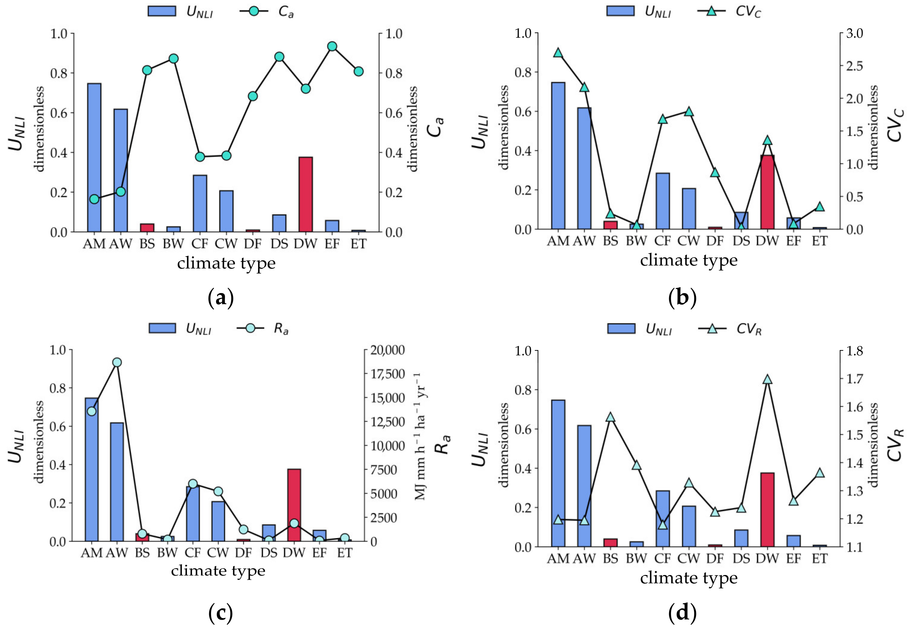
3.3. Soil Erosion after Köppen Climate Classification

According to the Köppen climate classification, there are 11 climate types in China, which are AM (tropical monsoon), AW (tropical savanna), BS (grassland), BW (desert), CF (humid warm), CW (dry warm winter), DF (constant wet cold warm), DS (dry summer cold and warm), DW (dry, cold and warm winter), EF (ice sheet), and ET (tundra). The climate types in most parts of southern China are CF and CW; the climate type in north-eastern China is DW and that in high-altitude areas such as Tibet is ET.

Figure 5 shows the monthly changes in R and C in six climate regions. Three pairs of climate zones were compared according to the similarity of the laws that display the changes in R and C throughout the year. For the first part (Figure 5a,b), although the R and C values differ considerably, the monthly fluctuation is similar. C reaches its lowest value in May–October. R peaks at the same time as C but at lower levels than C at other times. A similar pattern is also observed in AW and CW regions. For the second part (Figure 5c,d), the values of R and C are similar; C is stable at high levels, whereas R is stable at low level and throughout the year. A similar pattern is observed in DS, BW, and ET regions. For the third part (Figure 5e,f), R and C of DW and DF have similar values; the lowest value of C is observed in May–September; R is stable at low values, with higher values in May–September.

The relationship between U_NLI, C_a, R_a, and the coefficients of variation (CV) of monthly R and C in each Köppen climate zone was determined based on the values presented in Figure 6 for 2018. The blue bars represent negative uncertainty in U_NLI, whereas the red bars represent positive uncertainty. The U_NLI values are large in the AM and AW regions and smaller than 0.4 in other areas. Except for the BS and DW regions, the U_NLI values of all other regions are negative. In Figure 6a, the cyan circles represent the value of C_a in different climatic zones. The C_a values in AM, AW, CF, and CW regions are significantly lower than those in other regions (0.7 to 0.9), indicating poor annual vegetation coverage in these areas. In Figure 6b, the cyan triangles represent CV_C (degree of dispersion of monthly C values) in different climatic zones. In AM, AW, CF, and CW, the CV_C values are high. Figure 6a,b shows that although the average vegetation coverage in some areas is poor throughout the year, the annual variations are significant. In regions where soil erosivity is less uncertain, such as BS, BW, DS, EF, and ET, CV_C is low, but in DF, this trend is not obvious. In Figure 6c, the blue circles represent the values of R_a in different climatic zones. The values of R_a in the AM and AW regions are large, whereas in other regions, R_a is less than 7500 mm. R_a and U_NLI are similar in each region except in DW. In Figure 6d, the blue triangles represent CV_R (degree of dispersion of monthly R) in different climatic zones. In regions where U_NLI is positive, such as BS and DW, CV_R is very high throughout the year, indicating that rainfall intensity changes greatly. However, CV_R in other regions is less than 0.5.

4. Discussion

Rainfall erosivity is the main driving force of sediment and nutrient loss worldwide, increasing the vulnerability of farmers to crop failures and leading to an unstable landscape [43,44]. Rainfall erosivity, which is a measure of the amount and intensity of rainfall, is most often expressed as the R-factor in the USLE and RUSLE [45]. Land use and management affect the extent of soil erosion, and cover and management are represented by the C-factor. Among different soil erosion risk factors, C-factors are the most influential for decision makers and farmers to help reduce soil loss rates. [46] Compared to the other factors of RUSLE, rainfall erosivity, and coverage management in different months have strong temporal variability. R is cumulative Xie, Yin, Liu, Nearing and Zhao [33], that is, if R remains unchanged, the soil erosion estimations in the same year would not be affected regardless of how R_m changes during the year. Although other factors can be calculated considering their own annual variations, RUSLE simply multiplies the five factors, which indicates that the equation has certain shortcomings. The influence of the regional vegetation growth cycle on soil erosion is not well reflected in the equation, which may increase the uncertainties in the estimates.

By matching the R and C values on a monthly scale, this study considers the vegetation growth cycle in the soil erosion estimation process and determines how it affects the results of the RUSLE. The difference in the vegetation growth cycle will directly affect the surface vegetation coverage and thus the value of the C-factor. Furthermore, the relationship between precipitation and the vegetation growth cycle in a region cannot be ignored. In the RUSLE, the R-factor is the main driving force of soil erosion, and the C-factor plays an important role in maintaining soil stability. In the method used in this study, the two factors together affect soil erosion, and the differences of the two methods are significant. In north-eastern and northern China, the results of the original RUSLE, A_a, are overestimated, while in southern China, they are underestimated. In the north-western inland areas, the U_EDI was low. Therefore, the difference between the winter and summer climate in some parts of China changes the vegetation growth cycle, which in turn affects the results of the RUSLE based on the C-factor.

To explore the influence of different vegetation growth cycles on the uncertainties in the results, we analysed R and C under different climatic conditions classified according to the Köppen climate classification method. The Köppen climate classification is currently one of the most widely used and most influential methods in the world. In addition to temperature and precipitation, it also uses the vegetation distribution to determine the boundary index values between climate types. It divides the world into five basic climate zones and 12 major climates. It is suitable for tundra, forest, grassland, desert, and other landscape belts [47]. The levels of R and C were significantly different from the annual transformation trend under different temperature, precipitation, and natural vegetation. Based on this difference in climate regions, this study further visualised the mean value, coefficient of variation of two factors, and U_NLI in each climate region. According to the results, the mean of R is directly proportional to U_NLI, while the mean of C is inversely proportional to U_NLI, and the coefficient of variation of C is directly proportional to U_NLI, while the coefficient of variation of R is not significantly related to U_NLI. China has a variety of climates, and vegetation under different climate types has different growth cycles; that is, if affected by vegetation growth cycle, the variations in C values in each climate region within a year are large. However, the RUSLE equation does not fully reflect the impact of this difference on the estimation results, so the intra-year difference of C and the way in which it interacts with R significantly affects the estimation of soil erosion and must be evaluated. Considering the changes in R and C in each climate zone, we initially indicated that the size of R would overestimate the uncertainty caused by the difference in C. In the southern part of China, the main vegetation type is subtropical evergreen broad-leaved forests, and the annual vegetation coverage is high. Therefore, C in southern China always has a low value, reaching 0 at the annual scale, for which the original equation does not consider the soil erosion caused by R in winter. However, due to the relatively poor environmental conditions in winter, C has a non-zero value, and thus, in this case, the actual soil erosion is generated by the winter R. Therefore, the traditional estimation of soil erosion in most regions of southern China is characterized by a strong underestimation.

In northern China, the climate type is temperate monsoon, where the R level is higher in summer and lower in winter, with significant seasonal variations. The dominant vegetation in northern China is temperate deciduous broad-leaved forest; thus, vegetation cover varies greatly during the year. The C value in the entire year is high, but due to the better growth during the summer, C has a value of 0 in summer. In addition, the actual amount of soil erosion is generated by the non-summer R. However, in the original equation, the higher C on the annual scale means that the calculation process considers the level of R for the entire year. The R of non-summer months is much smaller than that of summer; thus, the soil erosion values in most areas of northern China are highly overestimated. The uncertainty in the soil erosion estimates is very low in areas where R is extremely low, but when C is significantly high, there is no obvious seasonal trend between the two. Other low uncertainty regions, such as the extensive areas of the Huanghuai Plain, the middle and lower reaches of the Yangtze River, the Liaohe Plain, and the Sichuan Basin and the scattered banded areas distributed in the south of the southeast hills and the Yunnan mountainous areas, are affected by the low values of LS, K, and P factors and soil invasion estimates, despite having high erosion factors. In summary, this rule applies where C reflecting vegetation cover inhibits the effect of R reflecting the rainfall on the soil erosion potential.

5. Conclusions

This study questioned the correctness of the simple multiplication of the R and C in the RUSLE equation. Assuming that the rainfall erosivity in summer is highest for the year, and surface vegetation coverage is better at this time, that is, the R_m is high in summer, and the C_m is low, then whether the simple multiplication of R and C can correctly assess soil erosion raises doubt. This study improves the current soil erosion estimations by considering the vegetation growth cycle obtained by matching R and C on a monthly scale and comparing them with the traditional RUSLE model. To describe the uncertainty in the RUSLE caused by the temporal variability of R and C, a new metric U_NLI was defined. The mean value and coefficient of variation were introduced to describe the time variations in R and C in each climate zone. Finally, the law of the influence of vegetation growth cycle on the uncertainty of soil erosion estimation was obtained. This result has a certain reference significance for improving the estimation accuracy of RUSLE model.

This study shows that the uncertainty in the RUSLE results is affected by the dynamics of R and C. Owing to monsoon climate in China, R and C have strong temporal variability, which leads to great uncertainty in soil erosion estimation results. Moreover, owing to the characteristics of C, the actual month of soil erosion is different from that considered in the original equation. On this basis, the value of R aggravates the impact of this difference on the uncertainty of the conventional soil erosion estimates. Therefore, under the monsoon climate, when C is low and its coefficient of variation is high, the few months that should have caused soil erosion were ignored in the original equation. In this case, the larger the R_m are in these months, the stronger the negative uncertainty of the calculated results. In addition, when both C and its coefficient of variation are high, the few months that should not have caused soil erosion are counted in the original equation. In this case, the larger the R_m in these months, the stronger the positive uncertainty of the calculated results.

The limitation of this study is that it only considers the uncertainty in the soil erosion estimates calculated using the RUSLE at the regional scale; thus, the findings are only applicable to specific regions. However, climatic conditions in different regions are different, as well as the corresponding vegetation growth cycles. We plan to expand the research scope to a global scale and consider the influence of different vegetation growth cycles. Furthermore, our goal is to establish a model for the combined effects of R and C on the uncertainty of soil erosion estimation to propose a suitable correction for the estimated result of the RUSLE equation.

References

1. Crosson, P. Soil Erosion Estimates and Costs. Science 1995, 269, 461–465. [Google Scholar] [CrossRef] [PubMed]
2. Dent, D. Global Environment Outlook: GEO 4. Environment for development. United Nations Environ. Programme Sect. B State Trends Environ. 1987, 2007, 81–114. [Google Scholar]
3. Pimentel, D.; Harvey, C.; Resosudarmo, P.; Sinclair, K.; Kurz, D.; McNair, M.; Crist, S.; Shpritz, L.; Fitton, L.; Saffouri, R. Environmental and economic costs of soil erosion and conservation benefits. Science 1995, 267, 1117–1123. [Google Scholar] [CrossRef] [Green Version]
4. Zhao, X.L.; Zhang, Z.X.; Zhou, Q.B. Soil erosion actuality and its synthesis prevention countermeasures in China. J. Soil Water Conserv. 2002, 16, 40–43. [Google Scholar]
5. Kaffas, K.; Hrissanthou, V. Computation of hourly sediment discharges and annual sediment yields by means of two soil erosion models in a mountainous basin. Int. J. River Basin Manag. 2019, 17, 63–77. [Google Scholar] [CrossRef]
6. Dai, Q.; Yang, Q.; Han, D.; Rico-Ramirez, M.A.; Zhang, S. Adjustment of radar-Gauge rainfall discrepancy due to raindrop drift and evaporation using the Weather Research and Forecasting model and dual-Polarization radar. Water Resour. Res. 2019, 55, 9211–9233. [Google Scholar] [CrossRef] [Green Version]
7. Wischmeier, W.H.; Smith, D.D. Predicting Rainfall Erosion Losses: A Guide to Conservation Planning; US Department of Agriculture: Washington, DC, USA, 1978.
8. Renard, K.G.; Foster, G.R.; Weesies, G.A.; Mccool, D.K.; Yoder, D.C. Predicting Soil Erosion by Water: A Guide to Conservation Planning with the Revised Universal Soil Loss Equation (RUSLE); US Department of Agriculture: Washington, DC, USA, 1997.
9. Feng, Q.; Zhao, W. The study on cover-Management factor in USLE and RUSLE: A review. Acta Ecol. Sin. 2014, 34, 4461–4472. [Google Scholar]
10. Hara, F.; Achab, M.; Emran, A.; Mahe, G. Hydrological processes and water security in a changing world Study of soil erosion risks using RUSLE Model and remote sensing: Case of the Bouregreg watershed (Morocco). In Proceedings of the Hydrological Processes and Water Security in a Changing World, Beijing, China, 16 September 2020. [Google Scholar]
11. Sahli, Y.; Mokhtari, E.; Merzouk, B.; Laignel, B.; Vial, C.; Madani, K. Mapping surface water erosion potential in the Soummam watershed in Northeast Algeria with RUSLE model. J. Mt. Sci. 2019, 16, 1606–1615. [Google Scholar] [CrossRef]
12. Li, J.; Sun, R.; Xiong, M.; Yang, G. Estimation of soil erosion based on the RUSLE model in China. Acta Ecol. Sin. 2020, 40, 3473–3485. [Google Scholar]
13. Yuan, L.; Zhou, Q. The application of cellular automata in simulating the spatial-temporal dynamic development process of soil erosion. Res. Soil Water Conserv. 2005, 12, 59–64. [Google Scholar]
14. Wenwu, Z.; Bojie, F.; Yihe, L.; Liding, C. Land use and soil erosion at multiscale. Prog. Geogr. 2010, 25, 24–33. [Google Scholar]
15. Dai, Q.; Zhu, J.; Zhang, S.; Zhu, S.; Han, D.; Lv, G. Estimation of rainfall erosivity based on WRF-derived raindrop size distributions. Hydrol. Earth Syst. Sci. 2020, 24, 5407–5422. [Google Scholar] [CrossRef]
16. Xu, H. A Methodology of Soil Erosion Evaluation on Slope System. Earth Sci. 1997, 6, 652–655. [Google Scholar]
17. Nunes, A.N.; Lourenço, L.; Vieira, A.; Bento-Gonçalves, A. Precipitation and erosivity in southern Portugal: Seasonal variability and trends (1950–2008). Land Degrad. Dev. 2016, 27, 211–222. [Google Scholar] [CrossRef]
18. Loureiro, N.; Coutinho, M. A new procedure to estimate the RUSLE EI30 index, based on monthly rainfall data and applied to the Algarve region, Portugal. J. Hydrol. 2001, 250, 12–18. [Google Scholar] [CrossRef]
19. Chen, M.; Voinov, A.; Ames, D.; Kettner, A.; Goodall, J.; Jakeman, A.; Barton, M.; Harpham, Q.; Cuddy, S.; DeLuca, C. Open web-distributed integrated geographic modelling and simulation to enable broader participation and applications (Position paper). Earth Sci. Rev. 2020, 207. [Google Scholar] [CrossRef]
20. Wang, G.; Gertner, G.; Liu, X.; Anderson, A. Uncertainty assessment of soil erodibility factor for revised universal soil loss equation. Catena 2002, 46, 1–14. [Google Scholar] [CrossRef]
21. Panagos, P.; Karydas, C.G.; Gitas, I.Z.; Montanarella, L. Monthly soil erosion monitoring based on remotely sensed biophysical parameters: A case study in Strymonas river basin towards a functional pan-European service. Int. J. Digit. Earth 2012, 5, 461–487. [Google Scholar] [CrossRef]
22. Wischmeier, W.H.; Smith, D.D. Rainfall energy and its relationship to soil loss. Eos Trans. Am. Geophys. Union 1958, 39, 285–291. [Google Scholar] [CrossRef]
23. Ferreira, V.; Panagopoulos, T. Seasonality of soil erosion under Mediterranean conditions at the Alqueva dam watershed. Environ. Manag. 2014, 54, 67–83. [Google Scholar] [CrossRef]
24. Yang, X. Deriving RUSLE cover factor from time-series fractional vegetation cover for hillslope erosion modelling in New South Wales. Soil Res. 2014, 52, 253–261. [Google Scholar] [CrossRef]
25. Angulo-Martínez, M.; Beguería, S. Estimating rainfall erosivity from daily precipitation records: A comparison among methods using data from the Ebro Basin (NE Spain). J. Hydrol. 2009, 379, 111–121. [Google Scholar] [CrossRef] [Green Version]
26. Ballabio, C.; Borrelli, P.; Spinoni, J.; Meusburger, K.; Michaelides, S.; Beguería, S.; Klik, A.; Petan, S.; Janeček, M.; Olsen, P. Mapping monthly rainfall erosivity in Europe. Sci. Total Environ. 2017, 579, 1298–1315. [Google Scholar] [CrossRef] [Green Version]
27. Wang, J.; Rich, P.M.; Price, K.P.; Wang, J.; Rich, P.M.; Price, K.P. Temporal responses of NDVI to precipitation and temperature in the central Great Plains, USA. International Journal of Remote Sensing. Int. J. Remote Sens. 2003, 24, 2345–2364. [Google Scholar] [CrossRef]
28. Durigon, V.L.; Carvalho, D.F.; Antunes, M.; Oliveira, P.; Fernandes, M.M. NDVI time series for monitoring RUSLE cover management factor in a tropical watershed. Int. J. Remote Sens. 2014, 35, 441–453. [Google Scholar] [CrossRef]
29. Baiamonte, G.; Minacapilli, M.; Novara, A.; Gristina, L. Time Scale Effects and Interactions of Rainfall Erosivity and Cover Management Factors on Vineyard Soil Loss Erosion in the Semi-Arid Area of Southern Sicily. Water 2019, 11, 978. [Google Scholar] [CrossRef] [Green Version]
30. Koo, H.; Iwanaga, T.; Croke, B.F.; Jakeman, A.J.; Yang, J.; Wang, H.-H.; Sun, X.; Lü, G.; Li, X.; Yue, T. Position paper: Sensitivity analysis of spatially distributed environmental models-a pragmatic framework for the exploration of uncertainty sources. Environ. Model. Softw. 2020, 134, 104857. [Google Scholar] [CrossRef]
31. Chen, C.; He, B.; Guo, L.; Zhang, Y.; Xie, X.; Chen, Z. Identifying critical climate periods for vegetation growth in the Northern Hemisphere. J. Geophys. Res. BioGeosci. 2018, 123, 2541–2552. [Google Scholar] [CrossRef]
32. Wischmeier, W.H.; Smith, D.D. Predicting Rainfall-Erosion Losses from Cropland East of the Rocky Mountains: Guide for Selection of Practices for Soil and Water Conservation; US Department of Agriculture: Washington, DC, USA, 1965.
33. Xie, Y.; Yin, S.Q.; Liu, B.Y.; Nearing, M.A.; Zhao, Y. Models for estimating daily rainfall erosivity in China. J. Hydrol. 2016, 535, 547–558. [Google Scholar] [CrossRef] [Green Version]
34. Yin, S.; Xie, Y.; Nearing, M.; Wang, C. Estimation of rainfall erosivity using 5-to 60-minute fixed-interval rainfall data from China. Catena 2007, 70, 306–312. [Google Scholar] [CrossRef]
35. Yan, Z.; Baoyuan, L.; Peijun, S.; Zhongshan, J. Crop cover factor estimating for soil loss prediciton. Acta Ecol. Sin. 2001, 21, 1050–1056. [Google Scholar]
36. Qi, J.; Marsett, R.; Moran, M.; Goodrich, D.; Heilman, P.; Kerr, Y.; Dedieu, G.; Chehbouni, A.; Zhang, X. Spatial and temporal dynamics of vegetation in the San Pedro River basin area. Agric. For. Meteorol. 2000, 105, 55–68. [Google Scholar] [CrossRef] [Green Version]
37. Cai, C.; Ding, S.; Shi, Z.; Huang, L.; Zhang, G. Study of applying USLE and geographical information system IDRISI to predict soil erosion in small watershed. J. Soil Water Conserv. 2000, 14, 19–24. [Google Scholar]
38. McCool, D.K.; Foster, G.R.; Mutchler, C.; Meyer, L. Revised slope length factor for the Universal Soil Loss Equation. Trans. Asae 1989, 32, 1571–1576. [Google Scholar] [CrossRef]
39. Liu, B.; Nearing, M.A.; Risse, L.M. Slope gradient effects on soil loss for steep slopes. Trans. Asae 1994, 37, 1835–1840. [Google Scholar] [CrossRef]
40. Williams, J.; Nearing, M.; Nicks, A.; Skidmore, E.; Valentin, C.; King, K.; Savabi, R. Using soil erosion models for global change studies. J. Soil Water Conserv. 1996, 51, 381–385. [Google Scholar]
41. Yaping, L.; Xiaoping, L.; Zhang, H.; Zezhong, L.; Wang, S. Soil erosion in Huaihe River Basin based on GIS and RUSLE:Exemplified by Shangcheng County, Xinyang City. Remote Sens. Land Resour. 2019, 31, 243–249. [Google Scholar]
42. Chen, S.; Yang, X.; Xiao, L.; Cai, H. Study of Soil Erosion in the Southern Hillside Area of China Based on RUSLE Model. Resour. Sci. 2014, 36, 1288–1297. [Google Scholar]
43. Panagos, P.; Borrelli, P.; Meusburger, K.; Yu, B.; Klik, A.; Lim, K.J.; Yang, J.E.; Ni, J.; Miao, C.; Chattopadhyay, N. Global rainfall erosivity assessment based on high-temporal resolution rainfall records. Sci. Rep. 2017, 7, 1–12. [Google Scholar] [CrossRef] [Green Version]
44. Wuepper, D.; Borrelli, P.; Finger, R. Countries and the global rate of soil erosion. Nat. Sustain. 2020, 3, 51–55. [Google Scholar] [CrossRef]
45. Panagos, P.; Borrelli, P.; Meusburger, K.; Alewell, C.; Lugato, E.; Montanarella, L. Estimating the soil erosion cover-management factor at the European scale. Land Use Policy 2015, 48, 38–50. [Google Scholar] [CrossRef]
46. Panagos, P.; Ballabio, C.; Borrelli, P.; Meusburger, K.; Klik, A.; Rousseva, S.; Tadić, M.P.; Michaelides, S.; Hrabalíková, M.; Olsen, P. Rainfall erosivity in Europe. Sci. Total Environ. 2015, 511, 801–814. [Google Scholar] [CrossRef] [PubMed] [Green Version]
47. Zhu, G.; Li, Y. Types and changes of Chinese climate zones from 1961 to 2013 based on Köppen climate classification. Arid Land Geogr. 2015, 38, 1121–1132. [Google Scholar]
Figure 1. Study area and position of rain gauges.
Land 10 00473 g001
Figure 2. Calculation of the annual cumulative rainfall erosivity (Ra) and annual land cover and management (Ca). (a) Calculation of Ra, (b) Calculation of Ca.
Land 10 00473 g002aLand 10 00473 g002b
Figure 3. Soil erosion in China (2018). (a) Soil erosion calculated using RUSLE, (b) Soil erosion calculated using RUSLE-dynaRC.
Land 10 00473 g003
Figure 4. UEDI value of soil erosion as the deviation between the soil erosion estimated in this study and the traditional RUSLE.
Land 10 00473 g004
Figure 5. Monthly changes of R and C values. (a) AM, (b) CF, (c) BS, (d) EF, (e) DW, (f) DF.
Land 10 00473 g005
Figure 6. UNLI in different climate zones. (a) Ca, (b) CVC, (c) Ra, (d) CVR.
Land 10 00473 g006