Exploring the Regional Dynamics of U.S. Irrigated Agriculture from 2002 to 2017

Abstract

The United States has a geographically mature and stable land use and land cover system including land used as irrigated cropland; however, changes in irrigation land use frequently occur related to various drivers. We applied a consistent methodology at a 250 m spatial resolution across the lower 48 states to map and estimate irrigation dynamics for four map eras (2002, 2007, 2012, and 2017) and over four 5-year mapping intervals. The resulting geospatial maps (called the Moderate Resolution Imaging Spectroradiometer (MODIS) Irrigated Agriculture Dataset or MIrAD-US) involved inputs from county-level irrigated statistics from the U.S. Department of Agriculture, National Agricultural Statistics Service, agricultural land cover from the U.S. Geological Survey National Land Cover Database, and an annual peak vegetation index derived from expedited MODIS satellite imagery. This study investigated regional and periodic patterns in the amount of change in irrigated agriculture and linked gains and losses to proximal causes and consequences. While there was a 7% overall increase in irrigated area from 2002 to 2017, we found surprising variability by region and by 5-year map interval. Irrigation land use dynamics affect the environment, water use, and crop yields. Regionally, we found that the watersheds with the largest irrigation gains (based on percent of area) included the Missouri, Upper Mississippi, and Lower Mississippi watersheds. Conversely, the California and the Texas–Gulf watersheds experienced fairly consistent irrigation losses during these mapping intervals. Various drivers for irrigation dynamics included regional climate fluctuations and drought events, demand for certain crops, government land or water policies, and economic incentives like crop pricing and land values. The MIrAD-US (Version 4) was assessed for accuracy using a variety of existing regionally based reference data. Accuracy ranged between 70% and 95%, depending on the region.

1. Introduction

Knowledge of the spatial and temporal dimensions of irrigated lands is useful for research, land/water management, and policy making. Understanding spatial and temporal trends of irrigated land can relate to the best agricultural practices and hence to better yields and better food supply. In short, consistent mapping of irrigated lands and understanding their dynamics can help in planning how to expand the food supply to the growing population, projected to reach 9.7 billion by 2050 [1].

Whereas croplands are dynamic and impractical to map at ground level because ground surveys are time consuming and costly, using remotely sensed imagery at various spatial and temporal resolutions to map and monitor rainfed or irrigated croplands is efficient and effective [2]. Various sources of satellite remote sensing contribute to mapping irrigated or rainfed crops. Moderate Resolution Imaging Spectroradiometer (MODIS) imagery with a temporal resolution of 1 day and spatial resolution of 250 m has been widely used to map cropland [3,4,5,6,7,8,9]. With its less frequent coverage but finer spatial resolution images, Landsat is also a popular source of data for mapping cropland. Some existing cropland maps include the Cropland Data Layer (CDL) produced by the U.S. Department of Agriculture (USDA) National Agricultural Statistics Service (NASS), the National Land Cover Database (NLCD) produced by the U.S. Geological Survey (USGS) [10,11], and Global Food Security-Support Analysis Data [12].

While mapping croplands (either as a whole or by mapping specific types of crops) is done by various federal agencies in the United States, relatively few datasets consistently identify temporal and spatial extents of irrigated croplands, which has formed a gap in the understanding of the dynamics of irrigated areas [5,8,13,14]. Mapping irrigated land is important because the spatial information of irrigated land can solve various challenges including understanding the effect of agriculture on water use, formulating effective management policies for this limited resource, and budgeting the agricultural water [8,14]. Fewer attempts have been made to map irrigated land at regional and/or contiguous United States (CONUS) level [5,8,15,16,17], and these are limited either by temporal or spatial constraints. The county-level irrigated area acreage documented by NASS, for example, lacks sub-county-level spatial information. The CONUS-wide 30 m LANID product by Xie et al. [17] is limited to a single year. Deines et al. [15] and Ketchum et al. [16] mapped irrigated areas for 30 years but were each limited to a single region—High Plains aquifer (HPA) and Western United States, respectively. The Moderate Resolution Imaging Spectroradiometer (MODIS) Irrigated Agriculture Dataset or MIrAD-US is the only product that has mapped irrigated area CONUS-wide for four eras (2002, 2007, 2012, and 2017). Even though the products are at coarser resolutions (250 m and 1 km), MIrAD-US provides consistent, accurate, and detailed geospatial information of irrigated area across the conterminous United States. [4,5].

In 2010, Pervez and Brown [8] developed a geospatial model to map irrigated agriculture across CONUS for 2002. This geospatial model incorporated the county-level irrigated statistics from USDA NASS with agricultural land cover from NLCD and the peak normalized difference vegetation index (NDVI) derived from 7-day expedited MODIS composites (eMODIS) at 250 m scale and is referred to as MIrAD-US. Later, the same approach was used by Brown and Pervez [5] to explore irrigation dynamics between two periods, 2002 and 2007. As an extension of these earlier efforts, we present the regional dynamics in U.S. irrigated lands for a 15-year period. We also accessed the accuracy of MIrAD-US at state and regional levels as per the availability of appropriate published reference data. The objectives of this study were to (1) examine the dynamics in U.S. irrigated area (using watersheds as a unit for analysis) and (2) assess the accuracy of the updated MIrAD-US product (version 4).

2. Background

We utilized a geospatial modeling strategy to create a multi-period CONUS-wide dataset for four eras (2002, 2007, 2012, and 2017) at a 250 m spatial resolution. In 2010, at the first publication of the 2002 map [8], existing studies were limited to 250 m resolution using MODIS, and repeat mapping did not occur. However, since that time technology has advanced, and new methods have been devised so that collection of CONUS-wide data at finer spatial resolution with a higher repeat cycle is possible. Various studies applied different approaches and methods to map irrigated land at finer resolution at larger temporal scales. Though limited to smaller regions, for example, the HPA region [15] or the Western United States [16], these studies were extended to a three-decade time period, whereas the study by Xie et al. [17] covered a larger region at a finer resolution but was limited to a single year. MIrAD-US is a coarser resolution CONUS-wide dataset for four periods at intervals of 5 years.

USDA NASS reported an increase in irrigated area between 2002 and 2007, a decrease in irrigated area between 2007 and 2012, and an increase in irrigated area between 2012 and 2017 across the United States [18]. This statistic is available at 5-year intervals at county level only and does not provide the spatial information of the irrigated area. Researchers who are seeking robust and comprehensive methods to produce detailed geospatial maps for irrigated areas found remote sensing to be the most successful technique for mapping irrigated land [5,8,15,17]. The use of remote sensing enables a diverse range of optimal spatial and temporal observational capabilities for a given study area. Remote sensing has the flexibility to widen and narrow the spatial and temporal scope of the study area. Though irrigated areas are mapped at different scales and for various regions, the studies on change dynamics in U.S. irrigated land are still limited. Earlier studies explored the irrigation pattern at particular states and/or regions [5,8,15,17] or ecoregions, but a national-scale watershed-level study of irrigation dynamics has not been conducted. This study also aimed to improve understanding of irrigation change dynamics across the United States at the level of major watersheds.

Watersheds provide a common geographic basis for understanding irrigated agriculture dynamics across the U.S. Watershed boundaries provide a seamless/standardized system where national hydrologic units are organized in a nested and hierarchical system using a unique code and represent the areal extent of surface water drainage to a single outlet [19]. The USGS Watershed Boundary Dataset (WBD) contains eight levels of progressive hydrological units identified by unique two- to 16-digit codes. We selected unique two-digit code hydrological units across CONUS at the most general level and collectively called them “watersheds” for this study. For further study, we selected 11 of these watersheds based on the dynamics and areal extent in irrigated areas between 2002 and 2017.

The two ways that water is supplied to cultivate crops are from direct rainfall and irrigation [20]. For irrigation, water is supplied either from surface water (via gravity flow from rivers, lakes, and reservoirs) or ground water (through springs or wells). While water availability is the most important factor for irrigation, other driving forces including types of irrigation, source of water, tariffs attached with water supply, the laws governing water-control [21], geographical location, land quality and physical attributes of the soil, and environmental parameters such as precipitation, temperature, and drought determine irrigation needs. Water supply for irrigation may be controlled at both local and regional levels by a state or an irrigation district [21]; therefore, it is crucial to understand the availability effects of these driving forces on irrigation. There are several studies that focus on evaluation of irrigation dynamics at local, state, and aquifer scales. While studies at watershed scale could help understand overall trend at a large scale providing more information on water availability (mostly surface water) surpassing the impacts of local variables, we found no studies at this scale. The aim of this study was to illuminate irrigation dynamics at a generalized watershed scale, which may be useful for understanding broader geographic patterns and developing regional water management strategies and hence combatting future food security threats.

3. Materials and Methods

3.1. Input Data/Geospatial Model

In developing an updated version of MIrAD-US (Version 4, [22]), we implemented the geospatial model developed by Pervez and Brown, using similar input sources but updating them to reflect current data availability [8] in order to map irrigated lands for four eras (2002, 2007, 2012, and 2017). Each MIrAD-US product corresponds with the year when USDA released their county-level irrigation area statistics data [18]. The other input data (eMODIS annual peak NDVI and NLCD) were selected from the same year or closest year, respectively. The guiding concept states (1) the irrigated crops show higher NDVI values than non-irrigated crops in the same local area; (2) both the irrigated and non-irrigated crops may exhibit similar NDVI values during optimum precipitation period (however, during drought the difference in NDVI between irrigated and non-irrigated crops may be maximized, and therefore, for this model to operate smoothly, ideally the annual time period with severe drought condition should be selected); and (3) the growing season peak NDVI, at any time it occurs, will vary for each crop and for each geographic region of the United States. Because the annual peak NDVI varies by crop, the model could be biased toward some of the peak NDVI values [8] as some crops tend to reach higher NDVI peaks than others. The best approaches to distinguish irrigated cells from the non-irrigated cells are either to compare with field data or compare wall-to-wall with United States crop maps [8]. A CONUS-wide detailed cropland specific dataset is not available for 4 mapping intervals, and producing field data is outside of our scope. Additionally, Pervez and Brown [8] investigated that whether peak NDVI would be a good indicator regardless of crop type at selected locations, and found it generally well supported. Further assessment of MIrAD-US by Wardlow and Callahan [23] of Nebraska irrigated agriculture also supported this finding.

In summary, the input data for our geospatial model include USDA county irrigation statistics, eMODIS annual peak NDVI, and land cover mask from NLCD [8]. First, 250 m eMODIS peak NDVI values were masked by resampled (250 m) NLCD data for agricultural land classes, then the peak NDVI were overlaid on county spatial data provided by the census. Then, a list of peak annual NDVI values was sorted in descending order. Starting with the highest ranked peak NDVI, the area of the corresponding peak NDVI value cells was computed and compared with the USDA irrigation area statistics for that county. The same process was repeated for each peak NDVI value in descending order until the accumulated area exceeded the county area estimate from the census [18]. The corresponding pixels that contribute to the matched area were identified as irrigated for the county. In a final post-processing step, all lone (single) pixels were spatially filtered from the irrigated area map.

3.2. Accuracy Assessment

We accessed the accuracy of MIrAD-US (Version 4) at different temporal and spatial extents depending upon the availability of reference data.

Table 1. Reference data used for accuracy assessment.

State/ Region	Spatial Coverage	Year	Corresponding MIrAD-US ra	Data Format	Source (URL/DOI)
California	All Counties	2002, 2006, 2008, 2012	2002, 2007, 2012	Polygon	https://water.ca.gov/ (accessed on 7 April 2021)
Washington	CPA	2012	2012	Points	Xie et al. [17]
Idaho	ESPA	2002, 2006, 2008, 2011	2002, 2007, 2012	Polygon	https://idwr.idaho.gov/ (accessed on 7 April 2021)
HPA Region	HPA–KS	2002	2002	Points	Deines et al. [13]
	HPA–NE	2005	2007	Points
	HPA–TX, NM, OK	2008, 2012	2007, 2012	Points
	HPA–CO	2016	2017	Points

HPA = High Plains aquifer, TX = Texas, NM = New Mexico, OK = Oklahoma, KS = Kansas, NE = Nebraska, CO = Colorado, ESPA = Eastern Snake River Plain aquifer, CPA = Columbia Plateau basin-fill aquifer.

lists the available reference data, area coverage, corresponding MIrAD-US year, and sources. As no new reference data collection was carried out by this effort, reference data were obtained from multiple sources including state agency irrigation, well databases, and data collected by other researchers. Some of these data were collected via survey, whereas some were derived from secondary sources using Google Earth Engine and remote sensing interpretation techniques. We refer to this collective dataset as “reference” data.

The temporal and spatial extent of reference data were not consistent with MIrAD-US; therefore, we matched the reference data year closest to MIrAD-US era and carried out accuracy assessment at state or region levels: For example, to validate MIrAD-2007 in California we used 2006 and 2008 reference data; to validate MIrAD-2017 in Colorado we used 2016 reference data; and to validate MIrAD-2007 and MIrAD-2017 for the HPA, we used 2008 and 2016 reference data, respectively.

Reference data for California for years 2002, 2006, 2008, and 2012 were obtained from the California Department of Water Resources (DWR). The DWR created digital vector field maps using visual interpretation of aerial photographs along with field visits. The 2002 reference data for the Eastern Snake River Plain aquifer (ESPA) (in vector format) were obtained from the Idaho Department of Water Resources (IDWR). We converted the IDWR irrigated lands vector database to raster format matching the spatial resolution of MIrAD-2002 and assigned 1 or 0 for irrigated and non-irrigated class based on the irrigation status information. Other reference data for the HPA for multiple years [13,15] and Columbia Plateau basin-fill aquifer (CPA) for 2012 [17] were developed using a semi-autonomous training approach in Google Earth Engine.

We applied the two most common and effective methods for accuracy assessment: (1) simple random and (2) stratified random. In the simple random method, the surveyed polygon fields were converted into grids using an irrigation attribute (1 for irrigated and 0 for non-irrigated) matching the spatial properties (projection, extent, and cell size) of MIrAD-US. Then, the MIrAD-US and new raster maps were overlaid with each other on a cell-by-cell basis and were made to have the same attribute values (e.g., 1 if the cell is irrigated and 0 if the cell is not irrigated). Second, a set of sample random points were created using the random point generator tool in ArcGIS [24]. These random points were constrained by the common areas from both data products, and any two points were minimally spaced at 1 km. Third, the random points were overlaid on a pixel-by-pixel basis with MIrAD-US raster and new raster, and irrigation information was extracted from the cell that contained the point. In the stratified random method, the irrigated (1) and non-irrigated (0) points were generated from the surveyed polygons instead. These points were overlaid on a pixel-by-pixel basis with MIrAD-US raster and irrigation information extracted from the cell that contained the point. Finally, an error matrix was generated using the extracted irrigation information from MIrAD-US to compute the following accuracies and errors: overall accuracy, user’s and producer’s accuracies, error of commission and omission, and kappa statistics.

Due to availability of surveyed polygons, stratified random methods of accuracy assessment were left out in the regions (e.g., CPA region, Table 1) with no polygon data.

4. Results

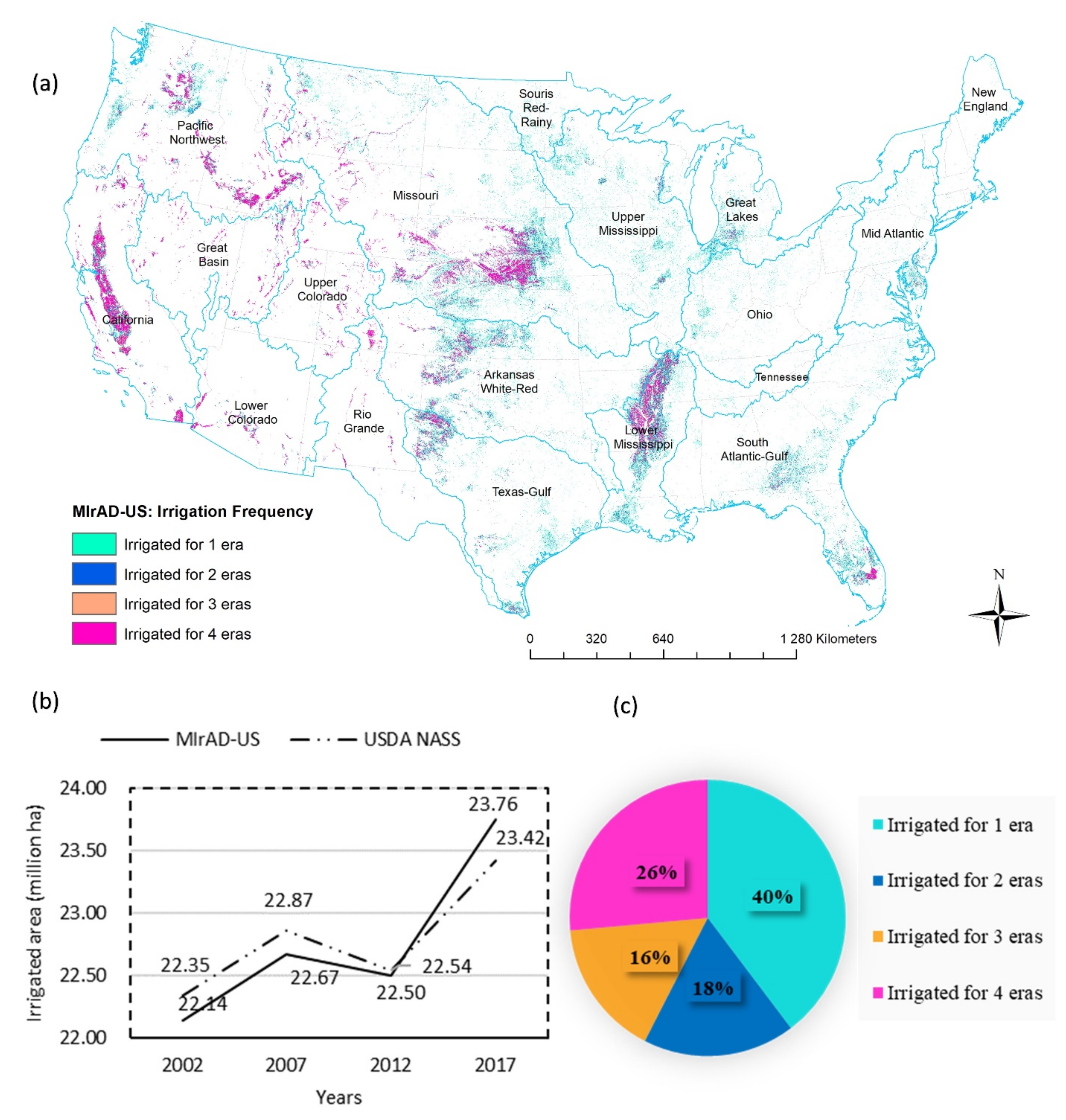
4.1. The MIrAD-US Dataset

The MIrAD-US is a source of geospatial raster data for irrigated land across the U.S. for four years at 250 m and 1 km resolution. All the products are projected into Lambert azimuthal equal area, saved in ArcGIS-friendly Geotiff format, and found in ScienceBase—an online portal maintained by USGS to store open data, repository services, and large datasets [22]. The MIrAD-US dataset has two classes: “irrigated” and “non-irrigated.” Similar to the Pervez and Brown [8] findings, most of the irrigated areas were concentrated in the Midwestern and Western United States and sparsely scattered throughout the more humid Eastern Seaboard and Mississippi Flood Plain in all four eras.

The MIrAD-US detected a gradual increase in irrigated area from 2002 (22.14 million hectares (mha)) to 2007 (22.67 mha), a slight decrease from 2007 to 2012 (22.50 mha), and a rapid increase from 2012 to 2017 (23.76 mha) (Figure 1b). The irrigation frequency maps (Figure 1a,c) show the majority of the lands (approx. 40%) were irrigated for 1 era followed by lands irrigated for 4 eras (approx. 26%). The South Atlantic–Gulf, Upper Mississippi, Great Lakes, Texas–Gulf, and a few parts of Missouri, Lower Mississippi, and Arkansas–White–Red watersheds were mostly irrigated for 1 era, suggesting unstable irrigation, whereas most of the lands in the Lower Mississippi, California, Missouri, and Pacific Northwest watersheds were irrigated for 4 eras, indicating a strong level of irrigation stability (Figure 1a). Lower precipitation rate and availability of water for irrigation can be associated with irrigation stability in these watersheds [25,26].

Table 2. Dynamics of the U.S. irrigated land between 2002 and 2017 at 5-year mapping intervals.

2002 and 2007
Irrigated Areas in ha		Common Areas between 2002 and 2007		Lost from 2002		New in 2007		Net Change in %
2002	2007	in ha	%	in ha	%	in ha	%
22,137,419	22,666,863	15,089,400	68.16	7,577,420	34.23	7,047,980	31.84	2.39
2007 and 2012
Irrigated areas in ha		Common areas between 2007 and 2012		Lost from 2007		New in 2012		Net change in %
2007	2012	in ha	%	in ha	%	in ha	%
22,666,863	22,497,394	15,158,800	66.88	7,338,630	32.38	7,508,100	33.12	−0.75
2012 and 2017
Irrigated areas in ha		Common areas between 2012 and 2017		Lost from 2012		New in 2017		Net change in %
2012	2017	in ha	%	in ha	%	in ha	%
22,497,394	23,755,163	15,158,800	67.38	7,508,100	33.37	7,338,630	32.62	5.59

shows areas of change and no change in irrigated land status between 2002 and 2017 at 5-year mapping intervals. Between 2002 and 2007, approximately 68.16% of the irrigated areas remained unchanged, 31.84% were newly identified in 2007, and 34.23% were identified as lost from 2002. Overall, there was a gain of 2.39% of irrigated land between these eras. The irrigated area decreased by -0.75% from 2007 to 2012 with approximately 66.88% of unchanged irrigated areas, 33.12% newly identified in 2012, and 32.38% lost from 2007 (Table 2). Between 2012 and 2017, irrigated area increased by 5.59% recording the highest gain in new irrigated areas among all mapping intervals. During this latest interval, approximately 67.38% of the irrigated areas remained unchanged, 32.62% was newly identified in 2017, and 33.37% was identified as lost from 2012 (Table 2).

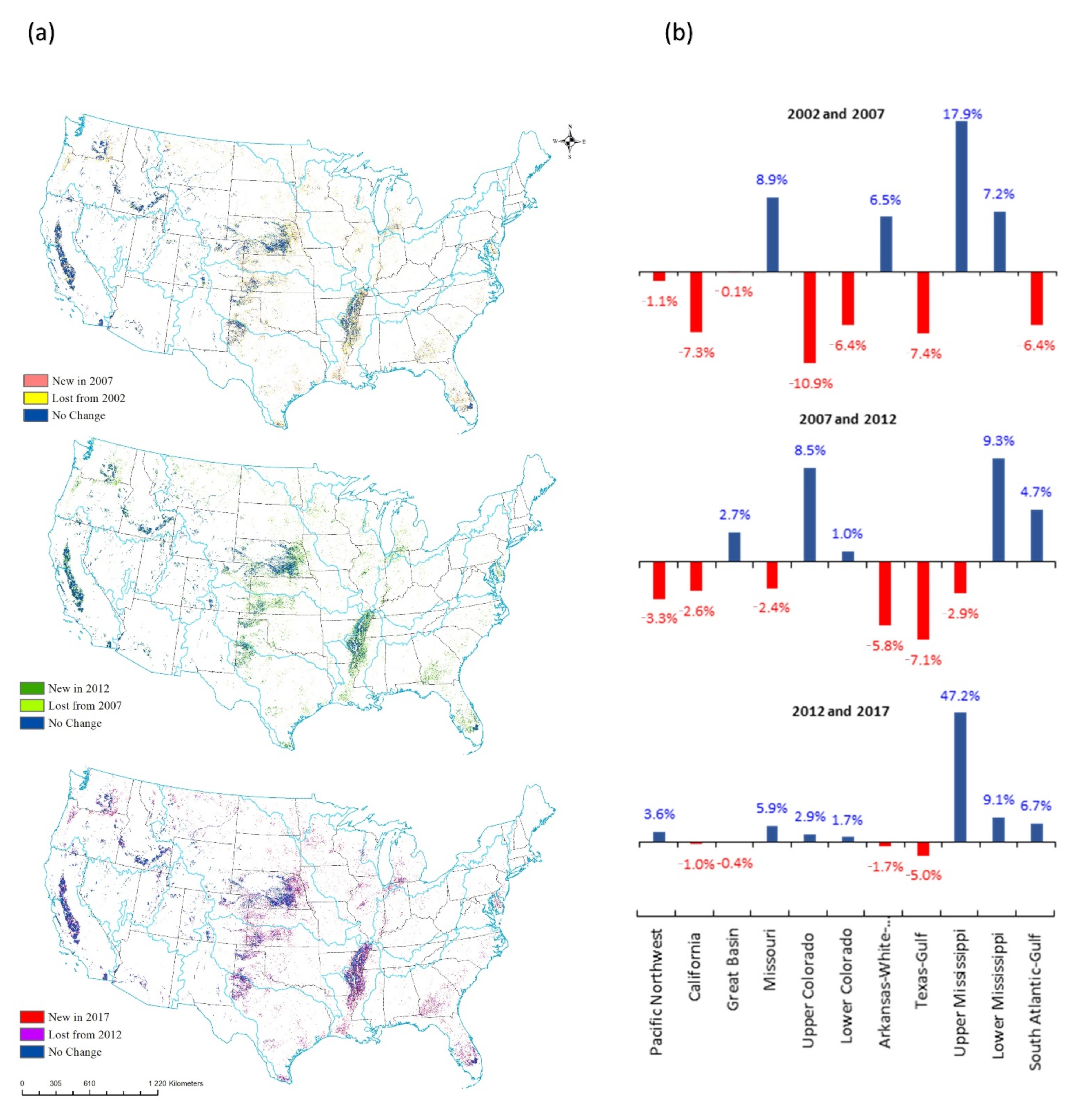
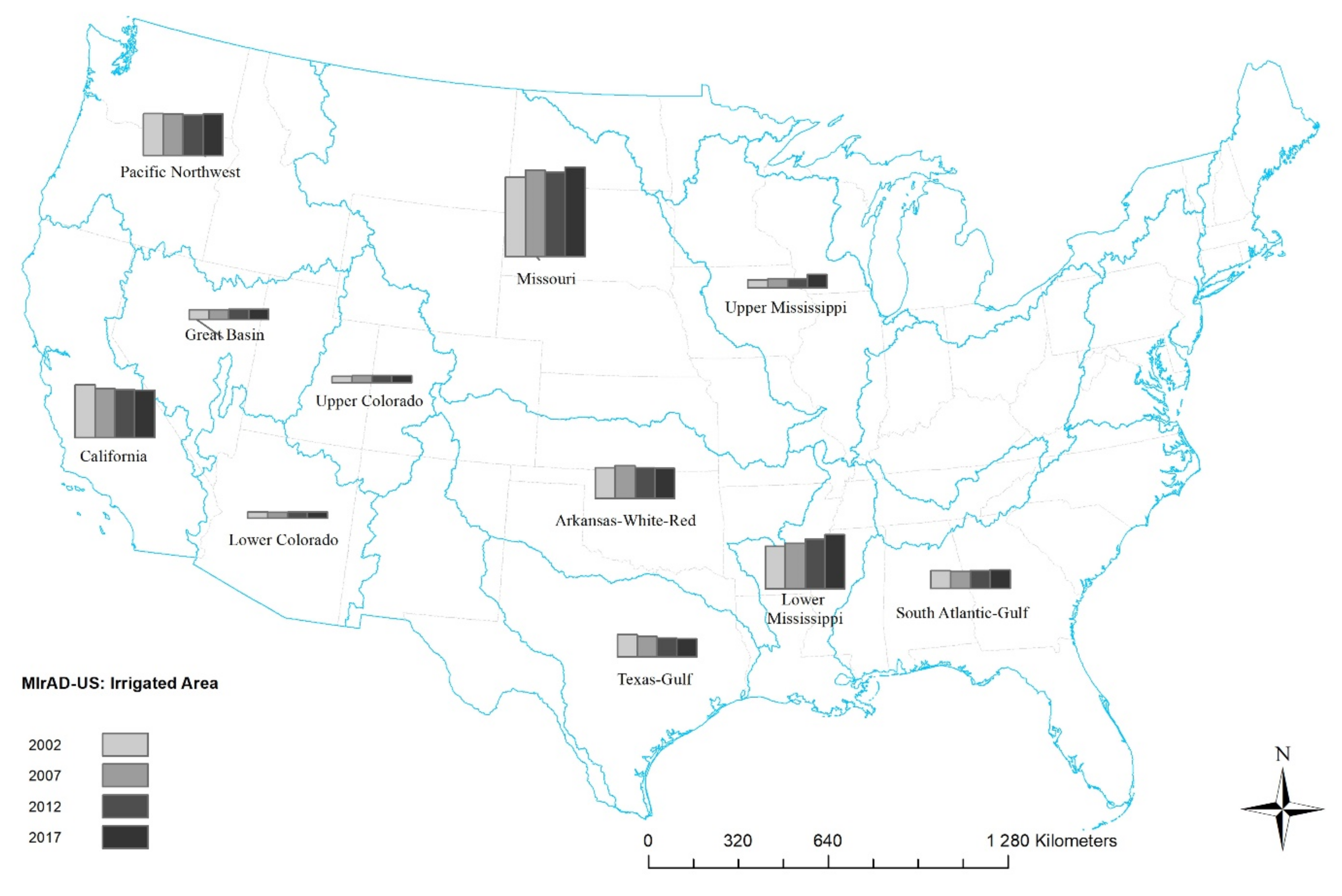
4.2. Watershed Dynamics in the U.S. Irrigated Agriculture from 2002 to 2017

Table 3. Change dynamics in the U.S. irrigated land between 2002 and 2017 at the watershed level.

Watershed Boundary Level MIrAD-US Irrigation Agricultural Land Estimates
2002 and 2007
Rank	Top 11 Watersheds	Irrigated Area in ha		Common Areas between 2002 and 2007		Lost from 2002		New in 2007		%▲
		2002	2007	in ha	%	in ha	%	in ha	%
1	Missouri	5,273,330	5,743,220	3,800,830	72.08	1,942,390	36.83	1,472,510	27.92	8.91%▲
2	Lower Mississippi	2,824,880	3,026,880	1,806,540	63.95	1,220,340	43.20	1,018,340	36.05	7.15%▲
3	California	3,523,890	3,268,110	2,937,490	83.36	330,619	9.38	586,400	16.64	−7.26%▼
4	Pacific Northwest	2,797,340	2,765,990	2,180,430	77.95	585,556	20.93	616,906	22.05	−1.12%▼
5	Arkansas–White–Red	2,041,760	2,174,680	1,180,210	57.80	994,463	48.71	861,550	42.20	6.51%▲
6	South Atlantic–Gulf	1,173,440	1,098,360	480,544	40.95	617,813	52.65	692,900	59.05	−6.40%▼
7	Texas–Gulf	1,479,090	1,369,590	815,181	55.11	554,413	37.48	663,913	44.89	−7.40%▼
8	Upper Mississippi	536,238	632,300	119,750	22.33	512,550	95.58	416,488	77.67	17.91%▲
9	Great Basin	640,856	640,213	555,463	86.68	84,750	13.22	85,394	13.32	−0.10%▼
10	Upper Colorado	487,700	434,419	402,175	82.46	32,244	6.61	85,525	17.54	−10.92%▼
11	Lower Colorado	429,919	402,394	353,781	82.29	48,613	11.31	76,138	17.71	−6.40%▼
2007 and 2012
Rank	Top 11 Watersheds	Irrigated Area in ha		Common Areas between 2007 and 2012		Lost from 2007		New in 2012		%▲
		2007	2012	in ha	%	in ha	%	in ha	%
1	Missouri	5,743,220	5,606,070	3,800,830	66.18	1,942,390	33.82	1,472,510	25.64	−2.39%▼
2	Lower Mississippi	3,026,880	3,309,190	2,305,370	76.16	1,303,410	43.06	1,003,830	33.16	9.33%▲
3	California	3,268,110	3,182,190	2,777,180	84.98	405,019	12.39	490,931	15.02	−2.63%▼
4	Pacific Northwest	2,765,990	2,673,740	2,114,000	76.43	559,744	20.24	651,988	23.57	−3.34%▼
5	Arkansas–White–Red	2,174,680	2,048,990	1,105,910	50.85	943,088	43.37	1,068,770	49.15	−5.78%▼
6	South Atlantic–Gulf	1,098,360	1,149,640	467,200	42.54	682,444	62.13	631,156	57.46	4.67%▲
7	Texas–Gulf	1,369,590	1,272,990	721,544	52.68	551,444	40.26	648,050	47.32	−7.05%▼
8	Upper Mississippi	632,300	614,225	129,394	20.46	484,831	76.68	502,906	79.54	−2.86%▼
9	Great Basin	640,213	657,213	572,313	89.39	84,900	13.26	67,900	10.61	2.66%▲
10	Upper Colorado	434,419	471,194	389,763	89.72	81,431	18.74	44,656	10.28	8.47%▲
11	Lower Colorado	402,394	406,319	352,063	87.49	54,256	13.48	50,331	12.51	0.98%▲
2012 and 2017
Rank	Top 11 Watersheds	Irrigated Area in ha		Common Areas between 2012 and 2017		Lost from 2012		New in 2017		%▲
		2012	2017	in ha	%	in ha	%	in ha	%
1	Missouri	5,606,070	5,937,240	3,949,610	70.45	1,656,460	29.55	1,793,610	31.99	5.91%▲
2	Lower Mississippi	3,309,190	3,608,780	2,070,288	62.56	1,238,906	37.44	956,594	28.91	9.05%▲
3	California	3,182,190	3,150,680	2,579,150	81.05	571,531	17.96	603,044	18.95	−0.99%▼
4	Pacific Northwest	2,673,740	2,770,780	2,077,500	77.70	693,275	25.93	596,244	22.30	3.63%▲
5	Arkansas–White–Red	2,048,990	2,013,760	1,024,560	50.00	989,200	48.28	1,024,430	50.00	-1.72%▼
6	South Atlantic–Gulf	1,149,640	1,226,600	485,656	42.24	740,944	64.45	663,988	57.76	6.69%▲
7	Texas–Gulf	1,272,990	1,209,180	649,963	51.06	559,213	43.93	623,025	48.94	−5.01%▼
8	Upper Mississippi	614,225	904,369	154,975	25.23	749,394	122.0	459,250	74.77	47.24%▲
9	Great Basin	657,213	654,563	578,600	88.04	75,963	11.56	78,613	11.96	−0.40%▼
10	Upper Colorado	471,194	484,800	427,194	90.66	57,606	12.23	44,000	9.34	2.89%▲
11	Lower Colorado	406,319	413,088	357,031	87.87	56,056	13.80	49,288	12.13	1.67%▲

and Figure 2a show the watersheds with the most substantial change in irrigated lands between 2002 and 2017. The statistics include the sum of irrigated area in each mapping interval (era); the sum and percentage of irrigated area lost from the preceding era; the sum and percentage of irrigated area gained in successive eras; and the sum and percentage of common area and net change between consecutive eras. The majority of irrigated lands (approx. 26%) across CONUS occurs in the Missouri watershed (Figure 2a). There, irrigated area increased from about 5.274 million ha in 2002 to about 5.94 million ha in 2017 (Table 3 and Figure 2b), which is roughly a 13% increase. During that time, the Missouri watershed gained about 8.9% irrigated area from 2002 to 2007, lost about −2.4% irrigated area between 2007 and 2012, and gained about 5.9% irrigated area between 2012 and 2017. The Upper and Lower Mississippi watersheds also experienced growth in irrigated lands, with the Lower Mississippi watershed consistently gaining about 7.2%, 9.3%, and 9.1% between these three intervals (Table 3), totaling 28% between 2002 and 2017. The Upper Mississippi watershed secured the highest percentage gain of 69% between 2002 (536,000 ha) and 2017 (904,000 ha) with about 17.9%, −2.9%, and 47.2% change between 2002 and 2007, 2007 and 2012, and 2012 and 2017, respectively (Figure 3). Because the actual magnitudes of irrigated areas were lower, the high percentage change did not contribute to overall change across the CONUS.

Watersheds suffering the greatest decreases in irrigation area include California and the Texas–Gulf (Table 3 and Figure 3). The California watershed lost about −7.3%, −2.6%, and −1% between map intervals with a total loss of about −11% between 2002 and 2017. The Texas–Gulf watershed faced the highest percentage loss of about −18% across the same time period.

California suffered from a prolonged drought and decreases in surface/ground water availability for irrigation throughout the study period leading to decreased irrigation, whereas the Missouri and Lower Mississippi watersheds still receive adequate ground water for irrigation. The increased number of ground water wells in Eastern Nebraska between 2002 and 2005 [8,15] and increased amount of rainfall in Lower Mississippi watershed from 1969 to 2017 [26] are driving factors for increased irrigation for these watersheds. Widespread drought in 2012 affected multiple watersheds like Missouri and California watersheds and resulted in an overall decrease in irrigation [27]. Between 2012 and 2017, increases in irrigated area in Missouri, Pacific Northwest, and Lower Mississippi watersheds offset the decrease in irrigation in the California watershed (Figure 2b).

4.3. MIrAD-US Product Accuracy

We collected reference data for accuracy assessment from multiple sources including state agencies, well databases, and data collected by other researchers (Table 1). Because these reference data were associated with different watersheds and time periods, the accuracy assessment task varied accordingly.

In California, we carried out the accuracy assessment for four eras and obtained overall accuracies above 95% (

Table 4. Error matrix summary of irrigated and non-irrigated category between MIrAD-US and reference data.

Region/ State	Ref. Year	Corr. MIrAD-US Era	Methods	Overall Accuracy	Omission Errors		Commission Errors		Total Points	Irr. Points
					Irr.	Non-Irr.	Irr.	Non-Irr.
California	2002	2002	Simple	94.93%	12%	4%	30%	1%	1557	158
			Stratified	64.10%	51%	21%	30%	39%	1997	998
	2006	2007	Simple	97.69%	9%	1%	10%	1%	1513	178
			Stratified	64.90%	53%	17%	27%	39%	1997	998
	2008	2007	Simple	95.34%	27%	1%	13%	4%	1608	197
			Stratified	63.08%	53%	21%	31%	40%	1991	996
	2012	2012	Simple	97.50%	17%	1%	7%	2%	2361	251
			Stratified	96.27%	4%	3%	4%	4%	4375	2014
Lower HPA (TX, NM, OK)	2008	2007	Stratified	81.97%	27%	8%	10%	24%	932	483
	2012	2012	Stratified	82.08%	30%	8%	13%	21%	865	388
HPA–KS	2002	2002	Stratified	62.02%	52%	17%	18%	49%	1498	915
HPA–NE	2005	2007	Stratified	80.15%	19%	20%	20%	20%	1950	989
HPA–CO	2016	2017	Stratified	70.82%	49%	9%	16%	35%	1004	497
ESPA	2002	2002	Simple	79.02%	17%	34%	10%	50%	1511	1191
			Stratified	65.96%	25%	43%	36%	31%	1992	998
CPA	2012	2012	Simple	81.00%	14%	22%	27%	12%	200	83

Ref. = reference, Corr. = corresponding, Irr. = irrigated, HPA = High Plains aquifer, TX = Texas, NM = New Mexico, OK = Oklahoma, KS = Kansas, NE = Nebraska, CO = Colorado, ESPA = Eastern Snake River Plain aquifer, CPA = Columbia Plateau basin-fill aquifer.

). The overall accuracies above 95% indicate that there was good agreement between DWR surveyed polygons and irrigated areas estimated by MIrAD-US. However, a relatively high commission error of roughly above 30% for the irrigated class and low omission error of roughly 12% indicate that, in this region where ground data were collected, MIrAD-US may have mapped more irrigated fields. For 2012, both random and stratified methods showed overall accuracies above 95% and omission errors below 17%, suggesting that there was a good agreement between surveyed data, and the irrigated areas were not omitted in MIrAD-2012.

In the HPA region (Table 4), the MIrAD-US agreed reasonably well with ground surveyed irrigated area information with an overall accuracy of 81.97%, 82.08%, and 80.15% at lower HPA (2008 and 2012) and Nebraska (2005). There was comparatively less agreement between MIrAD-US and ground surveyed irrigated area information with an overall accuracy of 62.02% in Kansas (2002) and 70.82% in Colorado (2005). The relatively high errors of omission (49%) and low errors of commission (16%) in HPA-CO indicate that there may have been fewer irrigated fields mapped by MIrAD-US. The differences in spatial detail between MIrAD-US and HPA-CO and the discrepancy between the MIrAD-US date (2016) and field survey dates (2017) likely resulted in high errors of omission and low errors of commission in this area. In the Western United States, the overall accuracy remained relatively lower in the ESPA region than CPA region. Using IDWR reference data, the ESPA assessment showed good agreement between the MIrAD-2002 and the reference area map with overall accuracies of about 79% and 66% using simple random and stratified random methods, respectively. In the CPA, the overall accuracy of 81% for MIrAD-2012 indicates that there was good agreement with Xie et al. [17] derived reference data. However, relatively high omission error of roughly 14% for the irrigated class indicates probable omission of irrigated areas in MIrAD-2012.

5. Discussion

Lack of consistent reference data across all of CONUS and during the same mapping eras for assessing the accuracy of the MIrAD-US maps limited the possibility of carrying out a single accuracy assessment across the entire CONUS; however, results of this study show MIrAD-US classifies irrigated area with a moderately high degree of accuracy. The overall accuracies across the assessed regions ranged from about 62% to 97%.

We assume that recent irrigation dynamics are mainly determined by the amount of available water supply for irrigation and crop types. In addition, other possible factors including economic incentives such as crop pricing and land values, the demand for corn related to development of biofuels, government policies related to water or land use, land availability, and regional climate fluctuations may influence irritation dynamics [5]. The trends we found in irrigation area vary across both temporal and spatial scales. Based on MIrAD-US map data, we detected an overall increase between 2002 and 2007, a decrease between 2007 and 2012, and another increase between 2012 and 2017 (Figure 1b). However, trends varied by geographic region. MIrAD-US showed decreasing area in California and the Texas–Gulf watersheds, an increasing irrigated area in Upper and Lower Mississippi watersheds, and both increasing and decreasing irrigated area in Missouri and Pacific Northwest watersheds (Figure 3).

The majority of the irrigated lands across CONUS (approx. 26%) falls in the Missouri watershed. The MIrAD-US detected increasing total irrigated area over the course of the study period of 12.6%, from 5.27 mha in 2002 to 5.94 mha in 2017, with the maximum irrigated area in 2017, and the minimum irrigated area in 2002. The irrigated areas in 2007 and 2012 totaled 5.74 and 5.60 mha, respectively. Increasing irrigated area in the Missouri watershed is likely associated with adaptation of improved irrigation techniques including new groundwater mining and sprinkler technologies [5,28]; registration of new wells, particularly in Nebraska [5]; crop insurance and federal subsidies [29,30,31]; and shift from non-crops and/or wheat farming to corn farming due to increased corn prices as a result of high demands on ethanol production [5,18,28,29,30,31,32,33]. Despite these drivers, the 2012 drought led to a decrease in irrigated areas, which may be associated with a scarcity of ground water limiting the number of fields that could be irrigated [13,15].

Watersheds that showed increasing irrigated areas include the Lower and Upper Mississippi watersheds. In the Lower Mississippi watershed, the irrigated area increased by 7.15% between 2002 and 2007, followed by 9.33% and 9.05% for following mapping intervals (Table 4). The net increase in irrigated land between 2002 and 2017 was 27.75%. The increase in irrigated acres in the Lower Mississippi watershed may be associated with the types of irrigation methods, precipitation patterns, water availability, and corn prices during the study period. Most of the irrigated land in the Lower Mississippi watershed is located at the Mississippi Alluvial Plain (MAP). The MAP is widely known for row crops including rice, corn, soybeans, and fish farms [19,25,26,34]. Because rainfall events typically occur outside of the growing season, water for irrigation is supplied from groundwater or surface water [26,35,36].

A study by Yasarer et al. [26] described increasing precipitation in the Lower Mississippi watershed from 1969 to 2017, with an average increase of about 0.03 inch per decade, whereas the ground water elevation, streamflow, total cropland, and harvested cropland have declined. Despite a decrease in stream flow and total cropland area, multiple studies detected increases in irrigated cropland [26,35,37]. The increase in irrigated area is associated with adoption of efficient irrigation methods where the existing furrow irrigation system (that accounts for 75% of the irrigated area) is coupled with computerized timers, flow meters, irrigation scheduling, soil moisture sensors, precision leveling, and tail water recovery systems [26,35]. These irrigation methods reduce water use and prevent overdraft of the ground water supply [35]. In addition, adequate rainfall recharges the groundwater. In a study by Kebede et al. [35], they established a correlation between increased corn prices relating to corn-based ethanol production in the mid to late 2000s with increased irrigated cropland in the Mississippi watershed [7,38,39]. Even though this watershed seems to have enough water for irrigation at present, streamflow depletion has raised concerns for the future of available groundwater resources, which might lead to ecosystem/water stress [26,40,41].

Watersheds that showed decreasing irrigated area include the California and Texas–Gulf watersheds. The California watershed lost the highest acreage of irrigated area of 373,210 ha (10.59%) during the entire study period—the largest decrease (approx. 7.26%) occurred from 2002 to 2007 (Table 4). Much of the irrigation in California relies on surface water (i.e., gravity irrigation), and water supply originates from snowpack in the Sierra Nevada Mountains. A series of droughts from 2003 to 2016 (particularly 2002–2004, 2007–2009, and 2012–2016) coupled with unusual warm winters [1,19,34] led to decreases in snowpack in the mountains and to surface water shortage resulting in decreases in irrigated cropland [42,43]. Just as in California, depletion of groundwater levels also led to decreasing irrigated areas (−18%) in the Texas–Gulf watershed over the years [5,44].

While the mapping resolution of the MIrAD-US overcomes some spatial issues presented in subpixel fractional irrigated areas, it has trouble identifying irrigated fields that are smaller than a 250 m cell [8]. Fields that are smaller than 250 m are either classified as irrigated (if the majority of neighboring cells are irrigated), potentially leading to overestimation, or as non-irrigated land (if the majority of neighboring cells are non-irrigated), potentially leading to underestimation. MIrAD-US provides an estimate rather than an exact rendering of irrigated lands. Use of higher resolution images such as 30 m Landsat or 10 m Sentinel-2 might overcome the spatial issues [15,16,17]. The MIrAD approach identified irrigation status, but a change in irrigation status does not necessarily identify a change (presence or absence) in irrigation equipment [5]. Different approaches would be needed to detect irrigation equipment, which could be explored in further research.

Higher resolution (e.g., 30 m) annual irrigation mapping may be more useful in exploring the dynamics of U.S. irrigated agriculture as these higher resolutions can provide precise field locations of smaller fields with higher accuracy [15,16,17,45]; however, because the majority of irrigated fields in the United States are generally larger than a single pixel (250 m × 250 m = 62,500 m²), the 250 m MIrAD-US data are still good for detailed geospatial information of irrigated areas across the conterminous United States [4,5]. In addition, because MIrAD-US provides consistent and accurate information of irrigated area across CONUS for 15 years at 5-year intervals, these datasets are important for estimating irrigated croplands [5,8].

6. Conclusions

This study investigated both regional and periodic increases and decreases in irrigated agriculture across the lower 48 U.S. states and more specifically at the watershed level. While there was a 7% overall increase in irrigated area across CONUS from 2002 to 2017, we found surprising variability by watershed and by 5-year map interval. Although the Missouri, California, and Lower Mississippi watersheds showed the most stable irrigation patterns via irrigation frequency maps, they depicted different trends. The California watershed showed a general decrease in irrigated area, the Lower Mississippi watershed showed increases over time, and the Missouri watershed showed an increase with a break in 2012. A series of drought events in California led to surface water shortage resulting in a decrease in irrigated cropland, whereas abundant rainfall and water availability led to increase in irrigated cropland in the Lower and Upper Mississippi watersheds.

Accuracy of the MIrAD-US (Version 4) ranged between 62% and 97%, depending on the region. The accuracies vary because of the irrigated field size, the density or homogeneity of irrigated lands within the agricultural setting, and the reference data used. In California where irrigated field sizes were fairly large and homogenous and reference data were collected by field survey, agreements as high as 97% occurred between reference data and MIrAD-US. Alternatively, in the CPA region where the reference data were developed using a semi-autonomous training approach in Google Earth Engine, the overall accuracy was comparatively lower (81%). Additionally, low numbers of irrigated samples in reference data affected the overall accuracy by stratified methods. The overall accuracies (stratified) varied at different geographical locations for the same era of data; for example, for MIrAD-2012, the overall accuracy for California is about 97%; HPA-TX, NM, OK is about 82%; and CPA is 81%. Climatic variance could have played a role in irrigation accuracy variability, but in order to perform a quantitative analysis of irrigation accuracy during different climate conditions, we would need reference data that were collected to represent larger variability in climate. In the most cases, we have reference data for only a single year. Future research could address this topic by providing access to multi-temporal reference data for irrigated agriculture while considering climatic condition as a variable for data collection.

We recognize that important advances have recently occurred in mapping and monitoring irrigated lands at higher spatial resolutions (e.g., 30 m) through time. Two studies by Deines et al. [15] and Ketchum et al. [16] are notable in that they offer an annual mapping periodicity at 30 m spatial resolution, but for smaller regions. Advancing these types of efforts to operational annual mapping across CONUS would be the next logical step. In addition, the collection of comprehensive reference data that represents high frequency and geographic coverage would also be a great benefit for robust accuracy assessment.

The MIrAD-US 2002, 2007, 2012, and 2017 era geospatial datasets have been used to support a broad variety of applications. Some of the applications include modeling/mapping irrigated area, agriculture and cropland, hydrological/water resource modeling, and meteorological modeling. The MIrAD-US was coupled with other variables including biophysical variables (NASS Quick Stat, NASS CDL, NLCD, and Soil Survey); climatic variables (Tmax, Tmin, and percp); remote sensing imageries (MODIS); and others (land use land cover, elevation, ecoregion type) to model and map irrigated land at regional, ecoregion, or global scale [3,46,47,48,49,50,51,52,53,54,55,56,57,58,59]. Data are available for download from the USGS ScienceBase website (doi:10.5066/P9NA3EO8). The datasets are available in GeoTiff file formats at two different cell sizes (250 m and 1 km) with appropriate metadata.

References

1. United Nations Department of Economic and Social Affairs. Growing at a Slower Pace, World Population is Expected to Reach 9.7 Billion in 2050 and Could Peak at Nearly 11 Billion Around 2100. 2019. Available online: https://www.un.org/development/desa/en/news/population/world-population-prospects-2019.html (accessed on 19 November 2020).
2. Johnson, D.M.; Mueller, R. The 2009 cropland data layer. Photogramm. Eng. Remote Sens. 2010, 76, 1201–1205. [Google Scholar]
3. Howard, D.M.; Wylie, B.K.; Tieszen, L.L. Crop classification modelling using remote sensing and environmental data in the Greater Platte River Basin, USA. Int. J. Remote Sens. 2012, 33, 6094–6108. [Google Scholar] [CrossRef]
4. Wardlow, B.D.; Egbert, S.L. Large-area crop mapping using time-series MODIS 250 m NDVI data: An assessment for the U.S. Central Great Plains. Remote Sens. Environ. 2008, 112, 1096–1116. [Google Scholar] [CrossRef]
5. Brown, J.F.; Pervez, M.S. Merging remote sensing data and national agricultural statistics to model change in irrigated agriculture. Agric. Syst. 2014, 127, 28–40. [Google Scholar] [CrossRef] [Green Version]
6. Howard, D.M.; Wylie, B.K. Annual crop type classification of the US Great Plains for 2000 to 2011. Photogramm. Eng. Remote Sens. 2014, 80, 537–549. [Google Scholar] [CrossRef]
7. Massey, R.; Sankey, T.T.; Congalton, R.G.; Yadav, K.; Thenkabail, P.S.; Ozdogan, M.; Sánchez Meador, A.J. MODIS phenology-derived, multi-year distribution of conterminous U.S. crop types. Remote Sens. Environ. 2017, 198, 490–503. [Google Scholar] [CrossRef]
8. Pervez, M.S.; Brown, J.F. Mapping Irrigated Lands at 250-m Scale by Merging MODIS Data and National Agricultural Statistics. Remote Sens. 2010, 2, 2388–2412. [Google Scholar] [CrossRef] [Green Version]
9. Zhang, L.; Feng, H.; Jin, N.; Zhang, T. Mapping irrigated and rainfed wheat areas using high spatial–temporal resolution data generated by Moderate Resolution Imaging Spectroradiometer and Landsat. J. Appl. Remote Sens. 2018, 12, 046023. [Google Scholar] [CrossRef]
10. Homer, C.; Dewitz, J.; Fry, J.; Coan, M.; Hossain, N.; Larson, C.; Herold, N.; McKerrow, A.; VanDriel, J.N.; Wickham, J. Completion of the 2001 National Land Cover Database for the conterminous United States. Photogramm. Eng. Remote Sens. 2007, 73, 337–341. [Google Scholar]
11. Xian, G.; Homer, C.; Fry, J. Updating the 2001 National Land Cover Database land cover classification to 2006 by using Landsat imagery change detection methods. Remote Sens. Environ. 2009, 113, 1133–1147. [Google Scholar] [CrossRef] [Green Version]
12. Teluguntla, P.; Thenkabail, P.S.; Oliphant, A.; Xiong, J.; Gumma, M.K.; Congalton, R.G.; Yadav, K.; Huete, A. A 30-m landsat-derived cropland extent product of Australia and China using random forest machine learning algorithm on Google Earth Engine cloud computing platform. ISPRS J. Photogramm. Remote Sens. 2018, 144, 325–340. [Google Scholar] [CrossRef]
13. Deines, J.M.; Kendall, A.D.; Hyndman, D.W. Annual Irrigation Dynamics in the U.S. Northern High Plains Derived from Landsat Satellite Data. Geophys. Res. Lett. 2017, 44, 9350–9360. [Google Scholar] [CrossRef]
14. Ozdogan, M.; Yang, Y.; Allez, G.; Cervantes, C. Remote Sensing of Irrigated Agriculture: Opportunities and Challenges. Remote Sens. 2010, 2, 2274–2304. [Google Scholar] [CrossRef] [Green Version]
15. Deines, J.M.; Kendall, A.D.; Crowley, M.A.; Rapp, J.; Cardille, J.A.; Hyndman, D.W. Mapping three decades of annual irrigation across the US High Plains Aquifer using Landsat and Google Earth Engine. Remote Sens. Environ. 2019, 233, 111400. [Google Scholar] [CrossRef]
16. Ketchum, D.; Jencso, K.; Maneta, M.P.; Melton, F.; Jones, M.O.; Huntington, J. IrrMapper: A Machine Learning Approach for High Resolution Mapping of Irrigated Agriculture across the Western U.S. Remote Sens. 2020, 12, 2328. [Google Scholar] [CrossRef]
17. Xie, Y.; Lark, T.J.; Brown, J.F.; Gibbs, H.K. Mapping irrigated cropland extent across the conterminous United States at 30 m resolution using a semi-automatic training approach on Google Earth Engine. ISPRS J. Photogramm. Remote Sens. 2019, 155, 136–149. [Google Scholar] [CrossRef]
18. U.S. Department of Agriculture. 2017 Census of Agriculture in Geographic Area Series; United States Department of Agriculture: Washington, DC, USA, 2019.
19. U.S. Geological Survey; U.S. Department of Agriculture; Natural Resources Conservation Service. Federal standards and procedures for the National Watershed Boundary Dataset (WBD). In Techniques and Methods 11-A3; U.S. Geological Survey: Reston, VA, USA, 2013. [Google Scholar]
20. Centers for Disease Control and Prevention, National Center for Emerging and Zoonotic Infectious Diseases (NCEZID), Division of Foodborne, Waterborne, and Environmental Diseases (DFWED). Types of Agricultural Water Use. 2016. Available online: https://www.cdc.gov/healthywater/other/agricultural/types.html (accessed on 19 November 2020).
21. Hutchins, W.A. Irrigation Districts, their organization, operation, and financing. In Technical Bulletin No. 254; United States Department of Agriculture: Washington, DC, USA, 1931. [Google Scholar]
22. Brown, J.F.; Howard, D.M.; Shrestha, D.; Benedict, T.D. Moderate Resolution Imaging Spectroradiometer (MODIS) Irrigated Agriculture Datasets for the Conterminous United States (MIrAD-US); U.S. Geological Survey Data Release; U.S. Geological Survey: Reston, VA, USA, 2019. [CrossRef]
23. Wardlow, B.D.; Callahan, K. A multi-scale accuracy assessment of the MODIS irrigated agriculture dataset (MIrAD) for the state of Nebraska, USA. GISci. Remote Sens. 2014, 51, 575–592. [Google Scholar] [CrossRef]
24. Esri.com. Tool Reference. 2021. Available online: https://pro.arcgis.com/en/pro-app/latest/tool-reference/data-management/create-random-points.htm (accessed on 5 January 2021).
25. Maupin, M.A.; Barber, N.L. Estimated Withdrawals from Principal Aquifers in the United States, 2000; Circular U.S. Geological Survey: Reston, VA, USA, 2000; 46p.
26. Yasarer, L.M.W.; Taylor, J.M.; Rigby, J.R.; Locke, M.A. Trends in Land Use, Irrigation, and Streamflow Alteration in the Mississippi River Alluvial Plain. Front. Environ. Sci. 2020, 8, 1–13. [Google Scholar] [CrossRef]
27. NOAA National Centers for Environmental Information (NCEI) U.S. Billion-Dollar Weather and Climate Disasters. Available online: https://www.ncdc.noaa.gov/billions/ (accessed on 7 March 2020).
28. Wallander, S.; Claassen, R.; Nickerson, C. The Ethanol Decade: An Expansion of U.S Corn Production, 2000-09. In Economic Information Bulletin; United States Department of Agriculture: Washington, DC, USA, 2011. [Google Scholar]
29. Reitsma, K.D.; Dunn, B.H.; Mishra, U.; Clay, S.A.; DeSutter, T.; Clay, D.E. Land-Use Change Impact on Soil Sustainability in a Climate and Vegetation Transition Zone. Agron. J. 2015, 107, 2363–2372. [Google Scholar] [CrossRef] [Green Version]
30. Shrestha, D. The Impacts of Land Use and Land Cover Change on Water Quality in the Big Sioux River Watershed: 2007–2016. In Department of Geography; South Dakota State University: Brookings, SD, USA, 2019. [Google Scholar]
31. Wright, C.K.; Wimberly, M.C. Recent land use change in the Western Corn Belt threatens grasslands and wetlands. Proc. Natl. Acad. Sci. USA 2013, 110, 4134–4139. [Google Scholar] [CrossRef] [PubMed] [Green Version]
32. Clay, D.E.; Clay, S.A.; Reitsma, K.D.; Dunn, B.H.; Smart, A.J.; Carlson, G.G.; Horvath, D.; Stone, J.J. Does the conversion of grasslands to row crop production in semi-arid areas threaten global food supplies? Glob. Food Secur. 2014, 3, 22–30. [Google Scholar] [CrossRef] [Green Version]
33. Napton, D.; Jordon, G. Agricultural Land Change in the Northwestern Corn Belt, USA: 1972–2007. Geol. Carp. 2011, 11, 65–81. [Google Scholar]
34. U.S. Government Accountability Office. Irrigated Agriculture Technologies, Practices, and Implications for Water Scarcity. In Technology Assessment; U.S. Government Accountability Office: Washington, DC, USA, 2019. [Google Scholar]
35. Kebede, H.; Fisher, D.K.; Sui, R.; Reddy, K.N. Irrigation Methods and Scheduling in the Delta Region of Mississippi: Current Status and Strategies to Improve Irrigation Efficiency. Am. J. Plant Sci. 2014, 05, 2917–2928. [Google Scholar] [CrossRef] [Green Version]
36. Massey, J.H.; Mark, S.C.; Epting, J.W.; Shane, P.R.; Kelly, D.B.; Bowling, T.H.; Leighton, J.C.; Pennington, D.A. Long-term measurements of agronomic crop irrigation made in the Mississippi delta portion of the lower Mississippi River Valley. Irrig. Sci. 2017, 35, 297–313. [Google Scholar] [CrossRef]
37. Killian, C.D.; Asquith, W.H.; Barlow, J.R.B.; Bent, G.C.; Kress, W.H.; Barlow, P.M.; Schmitz, D.W. Characterizing groundwater and surface-water interaction using hydrograph-separation techniques and groundwater-level data throughout the Mississippi Delta, USA. Hydrogeol. J. 2019, 27, 2167–2179. [Google Scholar] [CrossRef] [Green Version]
38. Smidt, S.J.; Haacker, E.M.; Kendall, A.D.; Deines, J.M.; Pei, L.; Cotterman, K.A.; Li, H.; Liu, X.; Basso, B.; Hyndman, D.W. Complex water management in modern agriculture: Trends in the water-energy-food nexus over the High Plains Aquifer. Sci. Total Environ. 2016, 566, 988–1001. [Google Scholar] [CrossRef] [PubMed] [Green Version]
39. Welch, H.L.; Green, C.T.; Rebich, R.A.; Barlow, J.R.; Hicks, M.B. Unintended Consequences of Biofuels Production? The Effects of Large-Scale Crop Conversion on Water Quality and Quantity; U.S. Geological Survey Open-File Report 2010-1229; U.S. Geological Survey: Seattle, WA, USA, 2010.
40. Barlow, J.R.; Clark, B.R. Simulation of Water-Use Conservation Scenarios for the Mississippi Delta using an Existing Regional Groundwater Flow Model; U.S. Geological Survey Scientific Investigations Report 2011-5019; U.S. Geological Survey: Seattle, WA, USA, 2011.
41. Barlow, P.M.; Leake, S.A. Streamflow Depletion by Wells: Understanding and Managing the Effects of Groundwater Pumping on Streamflow; U.S. Geological Survey Circular: Reston, VA, USA, 2012.
42. McGuire, V.L. Water-level changes in the High Plains aquifer, predevelopment to 2009, 2007–08, and 2008–09, and change in water in storage, predevelopment to 2009. In Groundwater Resources Program; U.S. Geological Survey Scientific Investigations Report 2011-5089; USGS: Reston, VA, USA, 2011. [Google Scholar]
43. Brown, J.F.; Howard, D.; Wylie, B.; Frieze, A.; Ji, L.; Gacke, C. Application-Ready Expedited MODIS Data for Operational Land Surface Monitoring of Vegetation Condition. Remote Sens. 2015, 7, 16226–16240. [Google Scholar] [CrossRef] [Green Version]
44. Carter, E.; Hain, C.; Anderson, M.; Steinschneider, S. A water balance based, spatiotemporal evaluation of terrestrial evapotranspiration products across the contiguous United States. J. Hydrometeorol. 2018, 19, 891–905. [Google Scholar] [CrossRef] [PubMed]
45. Field, J.L.; Marx, E.; Easter, M.; Adler, P.R.; Paustian, K. Ecosystem model parameterization and adaptation for sustainable cellulosic biofuel landscape design. GCB Bioenerg. 2016, 8, 1106–1123. [Google Scholar] [CrossRef]
46. Jaeger, K.L.; Sando, R.; McShane, R.R.; Dunham, J.B.; Hockman-Wert, D.P.; Kaiser, K.E.; Hafen, K.; Risley, J.C.; Blasch, K.W. Probability of Streamflow Permanence Model (PROSPER): A spatially continuous model of annual streamflow permanence throughout the Pacific Northwest. J. Hydrol. X 2019, 2, 100005. [Google Scholar] [CrossRef]
47. Jin, Y.; Randerson, J.T.; Goulden, M.L. Continental-scale net radiation and evapotranspiration estimated using MODIS satellite observations. Remote Sens. Environ. 2011, 115, 2302–2319. [Google Scholar] [CrossRef] [Green Version]
48. Kipka, H.; Green, T.R.; David, O.; Garcia, L.A.; Ascough, J.C., II; Arabi, M. Development of the Land-use and Agricultural Management Practice web-Service (LAMPS) for generating crop rotations in space and time. Soil Tillage Res. 2016, 155, 233–249. [Google Scholar] [CrossRef]
49. Nguyen, T.H.; Nong, D.; Paustian, K. Surrogate-based multi-objective optimization of management options for agricultural landscapes using artificial neural networks. Ecol. Model. 2019, 400, 1–13. [Google Scholar] [CrossRef]
50. Pei, L.; Moore, N.; Zhong, S.; Kendall, A.D.; Gao, Z.; Hyndman, D.W. Effects of Irrigation on Summer Precipitation over the United States. J. Clim. 2016, 29, 3541–3558. [Google Scholar] [CrossRef]
51. Salmon, J.M.; Friedl, M.A.; Frolking, S.; Wisser, D.; Douglas, E.M. Global rain-fed, irrigated, and paddy croplands: A new high resolution map derived from remote sensing, crop inventories and climate data. Int. J. Appl. Earth Observ. Geoinf. 2015, 38, 321–334. [Google Scholar] [CrossRef]
52. Seyoum, W.M.; Milewski, A.M. Monitoring and comparison of terrestrial water storage changes in the northern high plains using GRACE and in-situ based integrated hydrologic model estimates. Adv. Water Resour. 2016, 94, 31–44. [Google Scholar] [CrossRef]
53. Tadesse, T.; Wardlow, B.D.; Brown, J.F.; Svoboda, M.D.; Hayes, M.J.; Fuchs, B.; Gutzmer, D. Assessing the Vegetation Condition Impacts of the 2011 Drought across the U.S. Southern Great Plains Using the Vegetation Drought Response Index (VegDRI). J. Appl. Meteorol. Climatol. 2015, 54, 153–169. [Google Scholar] [CrossRef]
54. Wylie, B.; Howard, D.; Dahal, D.; Gilmanov, T.; Ji, L.; Zhang, L.; Smith, K. Grassland and Cropland Net Ecosystem Production of the U.S. Great Plains: Regression Tree Model Development and Comparative Analysis. Remote Sens. 2016, 8, 944. [Google Scholar] [CrossRef] [Green Version]
55. Xin, Q.; Gong, P.; Yu, C.; Yu, L.; Broich, M.; Suyker, A.E.; Myneni, R.B. A Production Efficiency Model-Based Method for Satellite Estimates of Corn and Soybean Yields in the Midwestern US. Remote Sens. 2013, 5, 5926–5943. [Google Scholar] [CrossRef] [Green Version]
56. Zaussinger, F.; Dorigo, W.; Gruber, A.; Tarpanelli, A.; Filippucci, P.; Brocca, L. Estimating irrigation water use over the contiguous United States by combining satellite and reanalysis soil moisture data. Hydrol. Earth Syst. Sci. 2019, 23, 897–923. [Google Scholar] [CrossRef] [Green Version]
57. Zeng, L.; Wardlow, B.D.; Tadesse, T.; Shan, J.; Hayes, M.J.; Li, D.; Xiang, D. Estimation of Daily Air Temperature Based on MODIS Land Surface Temperature Products over the Corn Belt in the US. Remote Sens. 2015, 7, 951–970. [Google Scholar] [CrossRef] [Green Version]
58. Aegerter, C. Modeling and Satellite Remote Sensing of the Meteorological Impacts of Irrigation during the 2012 Central Plains Drought. In Dissertations & Theses in Earth and Atmospheric Sciences; University of Nebraska: Lincoln, NE, USA, 2016. [Google Scholar]
59. Peterson, D.; Whistler, J.; Egbert, S.; Brown, J.C. Mapping irrigated lands by crop type in Kansas. In Proceedings of the Pecora 18-Forty Years of Earth Observation: Understanding a Changing World, Herndon, VA, USA, 14–17 November 2011. [Google Scholar]
Figure 1. MIrAD-US estimations of irrigated land across CONUS: (a) map showing the CONUS-wide distribution of irrigation frequency for four eras where blue polygons represent CONUS-wide HUC2 watershed boundaries and light blue, dark blue, light orange, and pink represent irrigated area for 1, 2, 3, and 4 eras, respectively (b) total irrigated area (in million ha) estimated by MIrAD-US and USDA NASS for four eras, and (c) pie chart showing percentage of frequency of irrigated land for four eras.
Land 10 00394 g001
Figure 2. MIrAD-US: Irrigation Dynamics across all intervals, (a) graphics showing CONUS-wide proportional irrigation gain and loss and (b) column charts showing watershed-wide irrigation gain and loss at 5 years mapping intervals.
Land 10 00394 g002
Figure 3. The graphics showing the sum of irrigated area in hectares estimated by MIrAD-US for Figure 2002. 2007, 2012, and 2017 across the CONUS at watershed boundary level.
Land 10 00394 g003