Communication

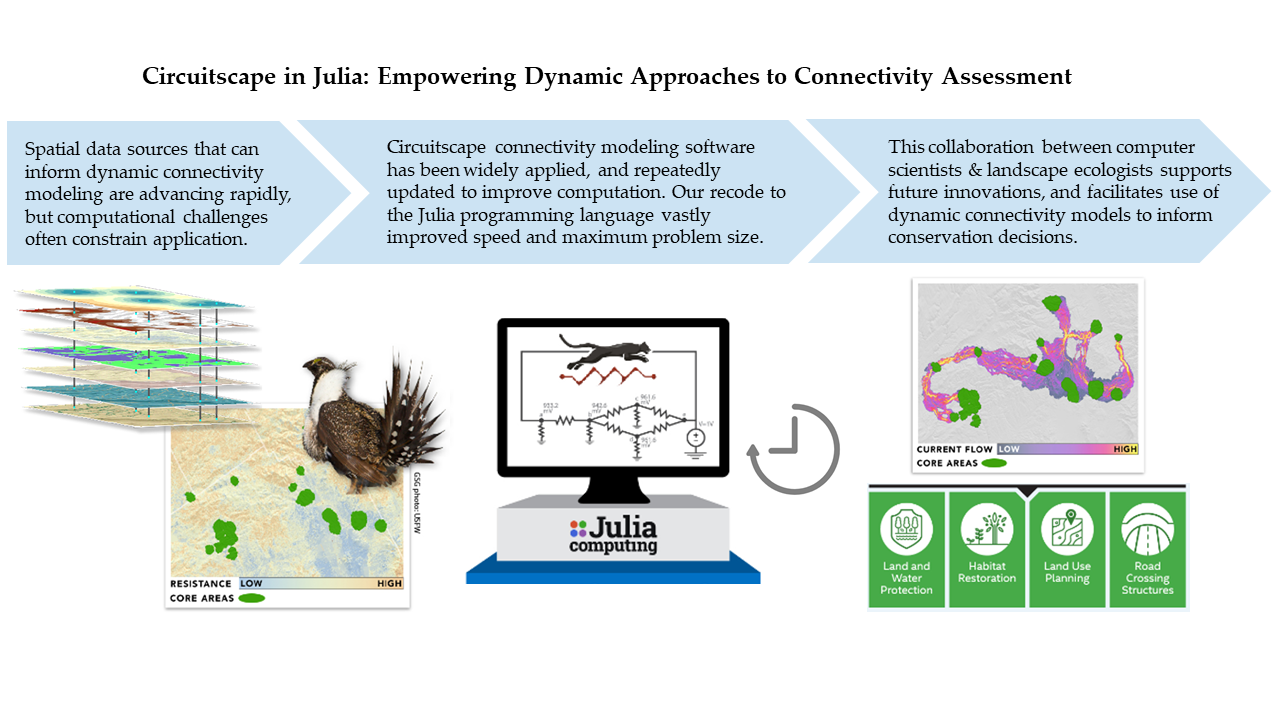
Circuitscape in Julia: Empowering Dynamic Approaches to Connectivity Assessment

1
North America Science, The Nature Conservancy, Haslett, MI 48840, USA
2
MIT Mathematics, Massachusetts Institute of Technology, Cambridge, MA 02139, USA
3
Conservation Science Partners, Inc., Fort Collins, CO 80521, USA
4
Center for Resilience Science, The Nature Conservancy, Boston, MA 02111, USA
5
Conservation Science Partners, Inc., Truckee, CA 96161, USA
6
Landscape Conservation Initiative, Northern Arizona University, Flagstaff, AZ 86011, USA
7
The Nature Conservancy, Santa Fe, NM 87501, USA
8
North America Science, The Nature Conservancy, Minneapolis, MN 55124, USA
9
Julia Computing, Inc., Cambridge, MA 02139, USA
*
Author to whom correspondence should be addressed.
Land 2021, 10(3), 301; https://doi.org/10.3390/land10030301
Submission received: 17 December 2020 / Revised: 9 March 2021 / Accepted: 10 March 2021 / Published: 15 March 2021
(This article belongs to the Special Issue Dynamic Landscape Connectivity)

Abstract

:
The conservation field is experiencing a rapid increase in the amount, variety, and quality of spatial data that can help us understand species movement and landscape connectivity patterns. As interest grows in more dynamic representations of movement potential, modelers are often limited by the capacity of their analytic tools to handle these datasets. Technology developments in software and high-performance computing are rapidly emerging in many fields, but uptake within conservation may lag, as our tools or our choice of computing language can constrain our ability to keep pace. We recently updated Circuitscape, a widely used connectivity analysis tool developed by Brad McRae and Viral Shah, by implementing it in Julia, a high-performance computing language. In this initial re-code (Circuitscape 5.0) and later updates, we improved computational efficiency and parallelism, achieving major speed improvements, and enabling assessments across larger extents or with higher resolution data. Here, we reflect on the benefits to conservation of strengthening collaborations with computer scientists, and extract examples from a collection of 572 Circuitscape applications to illustrate how through a decade of repeated investment in the software, applications have been many, varied, and increasingly dynamic. Beyond empowering continued innovations in dynamic connectivity, we expect that faster run times will play an important role in facilitating co-production of connectivity assessments with stakeholders, increasing the likelihood that connectivity science will be incorporated in land use decisions.

Graphical Abstract

1. Introduction

The conservation field is experiencing a rapid increase in the amount, variety, and quality of spatial data that can help us understand the dynamics of ecological systems, and incorporate key aspects of variation into land use decisions [1,2,3,4]. The accelerating pace of advances in the spatial and temporal resolution of ecologically relevant datasets track technology developments in remote sensing technologies, and in software and high-performance computing [5,6]. Updated software, and access to cloud computing and other high-performance hardware such as computing clusters and Graphics Processing Units (GPUs) are essential tools of the trade for researchers in other fields like data science and artificial intelligence that are experiencing similar explosions in data availability [7]. However, for landscape modelers who are collaborating and co-developing analyses with stakeholders and local governments, uptake of new science and technological advances may move slowly [8], especially when implementing change means leaving behind familiar tools or workflows. In this era of rapid global change, and concurrent leaps forward in data quality and availability, partnerships between conservation scientists and computer scientists that lead to updates of widely used, open-source software can help modelers keep pace, and more effectively support conservation decisions [7,9].
Here, we focus on assessments of landscape connectivity and animal movement potential, a conservation field that exemplifies the exciting opportunities and computational challenges that accompany improvements in technology. Recent advances in remote sensing and image processing have led to critically important increases in the variety of Earth observations available for characterizing the environment (e.g., types of ecological indicators and climatic variables, and options for spatial and temporal resolution), and advances in animal tracking technology are providing time series data on animal locations that can be integrated with environmental data [1,10,11]. Growth in citizen science efforts (e.g., eBird [12]), the deployment of automated data collection networks (e.g., camera traps, acoustic monitoring networks), and data sharing portals (e.g., Movebank [13]) are further increasing the volume of animal observation data streams [2].
The specific goals and underlying theories for landscape connectivity and animal movement models are many and varied [14]. Similarly, many different analytical approaches, software tools, and workflows are deployed to integrate geospatial data and ecological observations to build connectivity models (e.g., [14,15,16,17,18,19]). For applications that explore how landscape characteristics such as landcover type, topography, and the presence of barriers influence movement potential, representing the landscape as a “resistance” grid is a common element [15,17,20,21]. Each pixel of this surface is assigned a weight (or cost), that reflects, for example, habitat use patterns for an individual species, the likelihood of mortality in different habitats, or the “naturalness” of the landscape [20,21,22,23,24]. The datasets and models used to create resistance surfaces again vary, depending on the application, data availability, and the study goal [17,20,21,22,23,24]. However, once the surface is created and used as input for a connectivity analysis, many modeling workflows share the trait of being constrained by computational demand [15,22,25,26], as representing spatial patterns in a cumulative process like connectivity requires extensive calculations, often across millions of pixels. If connectivity modeling software crashes or requires weeks to run, these performance issues limit the scope and scale of our work.
Yet, for many important connectivity questions, we have the data to rapidly advance our understanding beyond a single snapshot (i.e., one resistance grid), and explore the dynamic nature of animal movement and other processes. Moving the field of connectivity science toward dynamic assessments has been identified as an important research priority, a goal that motivated this Special Issue [27,28,29,30]. In our contribution, we focus on the essential role that partnerships between ecologists and computer scientists can play in shaping this rapidly growing branch of conservation science, drawing from the history of improvements in and applications of Circuitscape [31].
For connectivity tools like Circuitscape that use resistance grids as inputs, shifting toward a more dynamic approach typically involves additional model runs on resistance surfaces parameterized for different seasons, climatic conditions, or landscape patterns. However, if the workflow to create a single output map is already constrained by computational requirements, adding more runs may not be feasible given time or resource constraints. Improvements to software can empower innovation by reducing these constraints, but as a general rule, the programming languages that enable higher performance are the most challenging to use. Here, we describe how a long-term partnership to improve Circuitscape supported rapid growth in the tool’s use, and also helped inspire a new high-performance programming language called Julia [32,33], which is now empowering the most recent Circuitscape release. We suggest that when improvements in software help users run computationally intensive models on available hardware (i.e., a personal computer, rather than a supercomputer), and are released as free, open-access tools, these investments play a key role in increasing accessibility, which can foster innovation, and the use of connectivity science to inform decisions. By describing this long-term collaboration, we hope to inspire ecologists to consider how similar improvements to other key tools could help the conservation community pursue more dynamic models, and take better advantage of rapid advances in the availability of ecological data.

2. Dynamic Approaches to Connectivity: Circuitscape Applications as a Case Study
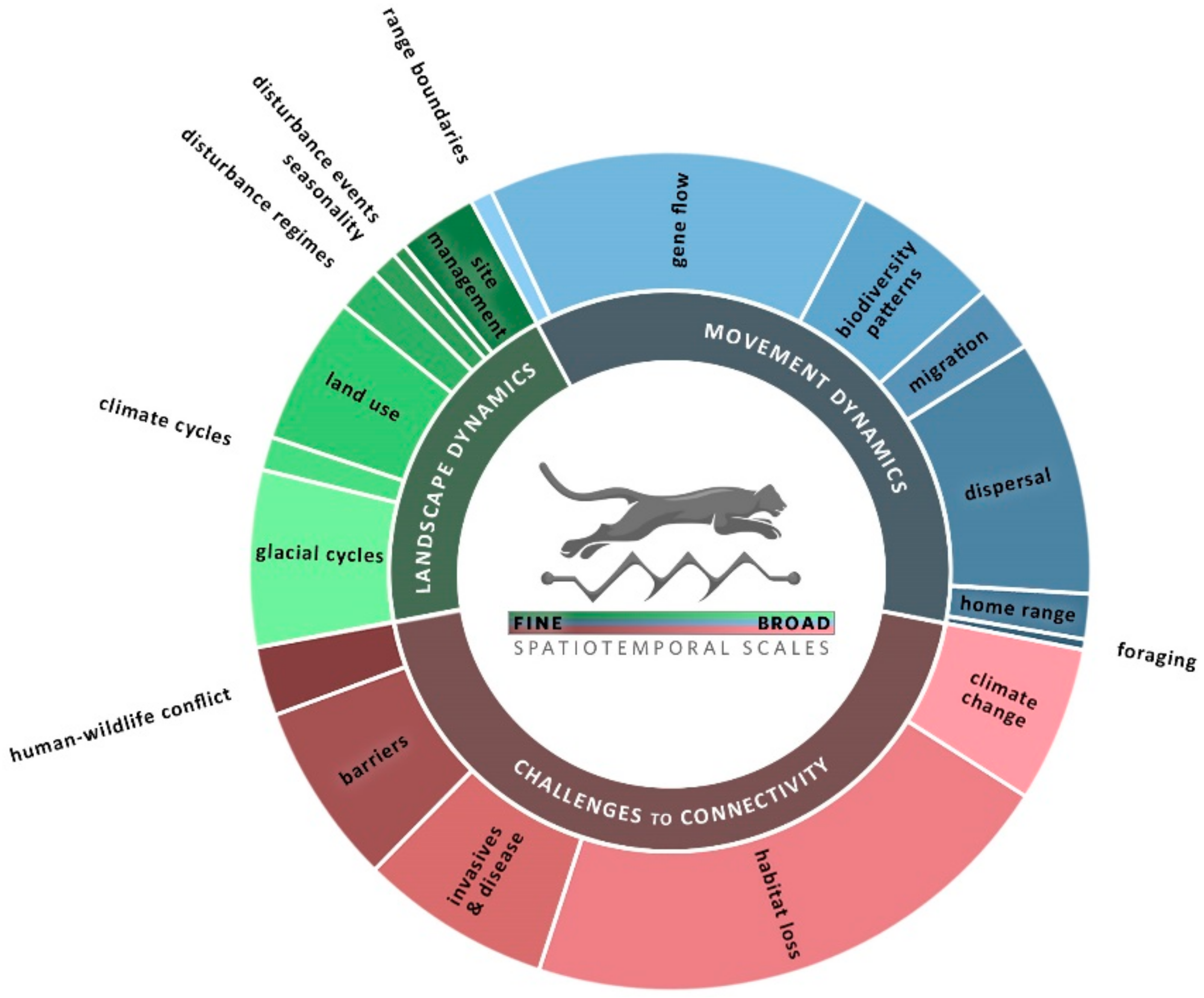
We recently updated Circuitscape [34], a widely used, open-source connectivity analysis software package, by migrating it from Python [35] to the Julia programming language [33]. Developed by conservation scientist Brad McRae (with a background in electrical engineering) and computer scientist Viral Shah, Circuitscape allows users to apply the logic and mathematics of electrical circuit theory to questions of how genes, animals, or processes flow across heterogeneous landscapes [22,31]. Briefly, this approach treats the landscape as a surface of resistors (the resistance grid). The Circuitscape algorithm tracks where “current” flows across this resistance surface, following current flow from source nodes to ground nodes, and quantifying the spatial patterns of current accumulation as higher resistance areas and barriers shift current flow into pathways with lower resistance [22]. This major update to Circuitscape was envisioned by McRae, but was carried out after his death in 2017. Initially developed to provide a tool for understanding the spatial dynamics of gene flow [36], Circuitscape has been applied in hundreds of connectivity studies on a wide range of organisms and topics, in locations across the globe. A recent review [16] and tributes [37,38] provide background on the underlying theory and history of Circuitscape’s development, and McRae’s influence within the fields of conservation and genetics. Circuitscape.jl (or 5.0 [34]), redesigned in the Julia language, represents a unique milestone in the long collaboration between McRae and Shah. First publicly released in 2012, the Julia programming language is still in rapid development [32,33] and was, in part, inspired by Shah’s experience collaborating with McRae to create a powerful yet accessible tool for biodiversity conservation applications.
The reach of Circuitscape reflects an unusual combination of innovative theory, analytical flexibility, and software accessibility. To date, Circuitscape has been most widely applied in landscape genetics, where modelers calculate “resistance distances,” a measure that indicates gene flow, between spatially referenced pairs of genetic samples [22,36,39]. As described above in an animal movement context, the spatial data surface(s) used as Circuitscape inputs typically represent habitat suitability, topography, climatic factors, or a composite surface, and resistance distance matrices may be calculated for one or many surfaces [20,24,40]. Later steps in the workflow focus on evaluating the relative support for each environmental dataset as a constraint on gene flow, a process that can involve multiple statistical modeling and optimization steps [41]. Some landscape genetics applications include resistance or current flow maps, but many do not—the measure of how environmental heterogeneity relates to genetic variation is typically the focal product. In contrast, in an animal movement context, producing current flow maps is the goal, with current magnitudes representing the relative use of different pixels by animals (or ecological processes) moving across the landscape (resistance surface) between focal nodes (habitat patches), following the assumption of a random walk [22].
Ecologists interested in animal movement questions have used a wide range of methods and models to create and assign weights to resistance surfaces, and these surfaces are typically developed from many spatial data inputs. Unlike applications in landscape genetics, which by their nature have a measure of past dispersal, the challenge of obtaining suitable animal movement data typically limits modelers’ abilities to directly evaluate weightings for animal movement models. This is an active area of research, and some modelers incorporate outputs from animal movement models into the development of the resistance grid (e.g., [17,42,43]), and/or develop outputs from other landscape connectivity models with different assumptions (e.g., least-cost path models) to contrast or complement Circuitscape’s assumption of a random walk (e.g., [44,45]). A third broad group of Circuitscape applications, including much of McRae’s work at The Nature Conservancy (TNC), emphasizes a generalized “structural” landscape connectivity that focuses on the pattern of land use, human influence, and barriers, and does not require the delineation of habitat patches to connect [46,47,48,49]. Like the species-focused maps, the structural outputs provide a way to visualize movement across landscapes as a cumulative process where both the magnitude and spatial pattern of resistance shapes how a generalized flow of organisms is channeled or spread out across multiple pathways, but source nodes are either aligned along the edges of the extent (e.g., [50]), or every pixel can be a source and ground (as in Omniscape [46,51], see Section 3, Section 4 and Section 5).
In support of the effort to update Circuitscape without McRae’s leadership, and inspired by the breadth of applications described in the Dickson et al. review [16], we assembled a comprehensive set of peer-reviewed Circuitscape applications. Our intent was to learn more about how the tool has been applied, to add to our list of potential new features for the software, and to identify potential new collaborators to help us keep building from McRae’s foundation. Our ongoing work with these applications includes examination of how computing constraints influenced modeling practices and spatial data use.
To find Circuitscape applications, we reviewed 1280 papers identified through Web of Science searches (end date for publication, including “early online” of December 2020, with the last search on 26 January 2021) that cited key foundational papers by McRae, Shah, and colleagues [22,31,36,39,46], or a Circuitscape user guide [25,52]. The user guides did not appear in searches by author, but we tracked them from the literature cited sections of a few applications; we found only a few studies that cited a user guide without also citing at least one of the foundational papers. From this set, we identified 572 papers in the natural sciences published in English from 2007–2020 where Circuitscape analyses were part of a research study. We included methods-focused papers if they had a case-study application; 11 papers that did not include a case study on a real landscape, as well as a few applications in other branches of science, were not included in our descriptions of applications. We did retain one paper in materials science [53], as it addressed issues of complexity that may be of interest to ecological modelers. In our counts by software version and topic, we did not attempt to control for the repeated use of the same Circuitscape analysis in different research papers. In a few cases the same paper used multiple versions of the software; we include these papers in the counts for both versions.
This set includes papers that used Circuitscape as part of another software package, such as Linkage Mapper [54], which has Circuitscape-based tools (Pinch Point Mapper and Centrality Mapper) in addition to tools for least-cost path analyses, and ResistanceGA [55] and Seraphim [56], software tools that can deploy Circuitscape to calculate pairwise resistance distances for genetics applications. We likely missed applications of Circuitscape in these tools, as we did not search for them directly, and thus only found them if the study cited one of the foundational papers. We did not include applications of gflow [57], a version of Circuitscape designed for deployment on supercomputers. This body of work represents an expansion over the 277 Circuitscape applications tallied in the Dickson et al. review [16], in part due to our identification of applications that only cited McRae’s first circuit-theory paper [36], a genetics-focused paper that was not traced in that review, and due to the extension of the search past that effort’s early 2018 end date. In just two years, the collection grew by over 180 papers (Figure 1a,b). The full list, including methods papers, is available as Supplementary Materials on https://Circuitscape.org/publications/.
The set of Circuitscape applications provides an interesting perspective on broad trends in the conservation field, including the expansion of dynamic connectivity approaches. There are many unique applications, but as described in Section 1, most Circuitscape analyses fall into three large and often overlapping categories—landscape genetic applications, studies that focus on movement potential for specific species or taxonomic groups, and structural connectivity approaches that provide a more general picture of how the arrangement of permeable land types and barriers shape movement potential (Figure 1a). We separated landscape genetics studies that provided a map(s) of resistance or current flow in the body of the paper (maps in supplements may have been missed) from those that did not, as these maps provide way to compare connectivity insights across multiple methods. Notably, as each Circuitscape application incorporates one or more resistance surfaces, the different methods used to construct these representations of the environment also provide an interesting view of a decade of changes in landscape ecology. For example, this collection illustrates the shift from patch dynamics toward consideration of matrix habitats, the rapid growth of the machine-learning based species distribution modelling tool Maxent [58,59], and the increasing use of remotely sensed data to understand ecological processes (e.g., [60,61,62]).
Figure 1. Count of Circuitscape applications in peer-reviewed journal articles by year, categorized by (a) type of application and (b) version of the software. Key milestones of each software version are indicated in the legend for (b). Graph (a) only includes genetic and movement-related applications (569); (b) includes 3 additional ecological applications, and one from materials sciences (573). A few studies used two versions of Circuitscape, and the count in (b) includes them under both software versions.
Land 10 00301 g001
While it is hard to draw a clear distinction between what is “dynamic” and what is “static” when comparing many diverse studies, it is easy to see that some applications are more dynamic than others. We found Zeller et al.’s dynamic connectivity framework (see Figure 2 in [30]) very helpful for organizing this compelling body of Circuitscape research. The dynamic connectivity framework identifies three categories, landscape dynamics, movement dynamics, and challenges to connectivity, and then presents sets of topics under each category that span a gradient of spatial and temporal scales. To help characterize the breadth and distribution of Circuitscape applications, we (KH) sorted the application papers following the framework, and present the resulting distribution across categories in Figure 2. We used the framework as a tool for grouping similar papers so that we could more easily highlight innovations in dynamic connectivity; as most papers could reasonably fit in more than one box, others would likely split them differently.
Although many Circuitscape applications are static, they are based on the dynamic concept of current flow across a network of resistors. For landscape genetics applications, each node in the network carries information on changes that occurred in the past; more dynamic applications include multiple genetic markers that provide insights from different time periods. For non-genetic applications, the dynamic nature of analyses can be greatly enhanced when modelers compare multiple representations of resistance (e.g., habitat change over time), or demographic or seasonal difference in how species respond to the landscape. The process of sorting and revising categories led to the identification of natural breaks in the set of papers, and we characterize those in Table 1. We used a few rules, including assigning papers that incorporated two movement types (e.g., home range and dispersal) or multiple challenges (e.g., habitat loss and climate change) in the larger-scale category. While nearly all landscape genetics approaches could reasonably be categorized as “gene flow,” the papers we grouped here emphasize a snapshot of the relationship between environmental patterns and genetic structure; when studies applied multiple genetic markers to capture change over time, or specifically addressed “challenges,” or “landscape dynamics” they were placed in other categories.
Figure 2. Distribution of 572 Circuitscape applications across the Zeller et al. [30] framing of topics in dynamic connectivity. Applications are grouped into three broad categories (inner circle), and then arranged in categories that range from finer scale (spatial or temporal) studies in darker shades, to applications at larger scales and/or longer focal time periods (lighter shades). See Table 1 for especially dynamic examples from these categories.
Land 10 00301 g002
For each topic, we present a brief phrase if needed to describe the studies in the category, and a few examples of dynamic study design approaches (Table 1). These factors show strong overlap with topics discussed in [30], such as including multiple time steps, demographic factors, movement types (habitat use vs. dispersal) and seasonal variations. For the studies we highlight, we indicate their “Circuitscape application type” (see Figure 1a) to show the overlap and unique contributions of each of these broad groups. To include the full set of Circuitscape applications, we added a “biodiversity patterns” category to the framework. We inserted this topic under movement dynamics to reflect studies where resistance distance measures from Circuitscape are applied to species assemblage data (or similar measures) to evaluate species turnover as a function of landscape heterogeneity (e.g., [63,64]). While we did not distinguish papers that incorporate genetic or animal movement data from multiple rather than a single species in Table 1 (as we did in Figure 1a for animal movement), we note this as a “dynamic factor” under a few of the topic areas. We found examples for all topics, though some topics have received much more coverage than others (Figure 2).
Table 1. Examples of dynamic elements within Circuitscape applications, as grouped in the dynamic connectivity topics presented in Zeller et al.’s framework [30]. The three main columns describe key research themes; topics are arranged according to focal temporal and spatial scales (large to small, see “scale” column), and the color scheme links columns to the same research themes and topics in Figure 2. Circuitscape application types are labeled as “LG” for landscape genetics, “MO” for species movement data & habitat models, and “ST” for studies focused on generalized landscape structure.
ScaleLandscape DynamicsMovement DynamicsChallenges to Connectivity
Longer time &
Larger
extent
Glacial cycles
Identify refugia & drivers of diversification [65,66,67,68]; detect a “glaciation signature” that provides context for current genetic variability [69,70,71] (LG).
Range boundaries
Use multiple genetic markers to capture environmental constraints across generational times steps [72] (LG); test multiple factors to identify constraints [73] (MO).
Climate change
Include projections of future climate [48,74,75,76,77] (ST & MO).

Consider niche space under paleo, current, and future climates [78,79,80]; evaluate adaptive capacity [81,82] (LG).

Integrate models of climate change & land use change [45,83,84,85,86] (ST, MO).
Climate cycles
Evaluate the influence of climate variability on gene flow (“isolation by instability”) [87,88,89] (LG). Includes the influence of ocean currents [90] (ST).
Gene flow
This group includes “snapshots” of genetic responses to heterogeneity. Also includes patterns in human language [91] & other distance-measurable traits.
Land use
Evaluate broad-scale changes in land use in time series data [49] (ST); capture the genetic impact of forest cover change (pollen sources) by sampling trees of different ages [92] (LG).

Model land use [93] (ST) or land function [94] (LG) scenarios, or the influence of land use policies [95] (ST).
Biodiversity patterns
Identify changes in species assemblages & turnover as a function of resistance. Can incorporate genetics, morphology [96].

Consider multiple time steps [97] or assess many sites in different landscape contexts [98]; in freshwater, consider the role of different hydrologic periods or [99] precipitation events [100].
Habitat loss/land use change
Consider multiple habitat configurations or loss scenarios [101,102,103,104]; integrate multiple species [105,106]; evaluate changes in a protected area network [107,108,109] (LG, MO).

Use multiple genetic methods to detect the influence of habitat loss relative to historical baselines [110,111,112,113,114,115,116] (LG).
Disturbance regimes & succession
Incorporate ocean currents & tidal influence [117,118,119] (LG & ST), fire regime [120], post-fire succession, [121] and dynamic (sand dunes) vs. static habitats [122] (LG).
Migration
Incorporate seasonal patterns or variation in resources [27,123,124,125,126] (MO).

Use multiple models to capture habitat choice and movement speed [42] (MO).
Invasive species & disease spread
Use information from multiple regions or introduction events [127]; pair time series of high-resolution habitat data with on-the ground detections of invasive species [62]; evaluate barrier strategies [128] (MO).

Use multiple waves to model viruses with wildlife vectors [129,130] (LG).

Consider how dynamics of pathogens & hosts may interact [131,132,133], and be influenced by humans [134,135] (LG).
Seasonality
Change in habitat patch configuration due to seasonal flooding/drought (ST) [61,136,137,138].

(see migration for many seasonality examples with movement data).
Dispersal
Recognize differences in home range use vs. dispersal [139,140,141,142] (MO); evaluate use of microclimates [40,143,144] (LG).

Incorporate life history variation, e.g., by sex [145,146], seed dispersal type [147], or response to conspecifics [148] (LG & MO).
Shorter time
&
Smaller
extent
Disturbance events
Disturbance events like fires can change dispersal patterns [149] (LG).

Consider hurricane routes as a driver of species colonization [150] (LG).
Home range
Consider variations by sex and/or seasons [151,152] (LG, MO), and the influence of social behavior [153] (MO).

Home range may include multiple habitat types [154,155]; agriculture can be a key connector [156,157] (MO).
Barriers to migration
Compare multiple sites [158,159] (LG); model current & future urbanization [160] or barrier removal [161] (MO), or passage structure locations [162] (MO).

Consider demographic differences in response to barriers (LG) [163,164].
Site restoration & management
Use scenarios to evaluate the targeting of fire risk mitigation [165] (ST) & vegetation management [166,167] (MO).

Integrate connectivity benefits & costs [168]; evaluate connectivity benefits of restoration [169] (MO).
Foraging
Consider differences in foraging mode (active vs. passive) [170] (LG).

Understanding reproductive timing may help scale the linkage between a dynamic resource and a focal species’ foraging range [171] (ST).
Human–wildlife conflict
Incorporate season & time of day in studies of road crossing risk [43] (MO). Simulate changes in barriers [172].

Integrate social science to understand the human side of conflicts [173,174] (MO).
As illustrated in Table 1, the collection includes applications at all scales, in freshwater, marine, and terrestrial environments. Less apparent from the table, which emphasizes alignment with the Zeller et al. framework, is the fact that the focal research subjects range in size from viruses and grains of pollen (e.g., [93,175]) through trees and elephants, and extend to work on human migrations and diseases, with a few applications integrating interactions between ecological and social systems (e.g., [173,174,176,177]). This diversity of scales and topics emphasizes Circuitscape’s role as a “springboard” for innovation [16], and a tool that helps ideas flow between different branches of environmental modeling.

3. Computation as a Constraint to Dynamic Models and Driver of Innovation

As indicated by the range of applications (Figure 2, Table 1), Circuitscape provides a very flexible platform for studying gene flow and connectivity, and we expect users will continue to advance the field by incorporating more dynamic approaches. However, the modeling process is very computationally intensive, a constraint that can limit how models are run, and the resolution of datasets that are deployed. To understand why computation can become a constraint, it’s helpful to understand that in a Circuitscape run, the landscape is represented by a grid of cells, and a resistive circuit is constructed by placing a resistor along the shared edge between every pair of neighboring cells. For a 1000 by 1000 resistance grid (1 million cells), the software will need computer hardware with enough processing power and memory to solve a system of 1 million linear equations [34]. In “pairwise” Circuitscape, the mode that is used to develop distance metrics for landscape genetics, and is commonly applied in animal movement studies, these calculations are repeated for every pair of nodes (for example, habitat patches or populations) included in the model. Our own experiences, and stories we have heard from other modelers, include Circuitscape computations that ran for days, and sometimes weeks. If the problem is too large for hardware resources (typically RAM, random access memory, is the limiting factor), the analysis will not run to completion. In this section, we discuss computational demand in the context of promoting more dynamic approaches to connectivity modeling, and also highlight modifications in how Circuitscape has been used that arose (at least in part) to address computational constraints. In Section 4, we introduce the Julia language version, and discuss how innovations in computer science and programming languages have great potential to help connectivity modelers track advances in the quality of spatial data, and implement more dynamic connectivity models.
Although the mathematics that describe changes in computational requirements as the resolution of input datasets increase are straightforward, in practice, this constraint is easy for connectivity modelers to overlook, especially when new, high-resolution data products are available. For example, if the 1 million cell landscape noted above is comprised of 1-km pixels (100 million ha, roughly the combined size of the US states of Utah, Colorado, Arizona, and New Mexico) and a modeler shifts to a data resolution of 500-m, that would typically quadruple the number of linear equations that need to be managed by the software and hardware. A more dramatic shift to a 30-m resolution dataset, the native resolution of many commonly used spatial data products, would increase the number of computations by a massive 1100×. The Circuitscape user guides [25,52] are clear on these computational challenges, and include warnings about total problem size, and sections on how to modify the input data and/or run parameters to reduce the potential for problems with RAM, or exceedingly long computation times. In the 572 Circuitscape ecological applications, roughly one-fourth discuss issues with computation and/or or describe aspects of their workflow that were designed to address computational issues. These types of modifications, and their potential influence, are part the focus of our ongoing review of this collection of papers. While our review is still underway, we found that at least 10% of authors reported aggregating pixels (reducing the resolution of the resistance grid), combining nodes (reducing the number of populations or patches to connect), or used some other tactic to address computational constraints. We expect that many more users experienced and addressed computation challenges than reported them.
For Circuitscape modelers who are considering more dynamic assessments, computation speed is of great practical concern, because accounting for seasonal variation, land use change, and other dynamic drivers requires multiple runs with different resistance grids. Most modelers featured in our dynamic examples (Table 1) have included several resistance grids, while a few of the most dynamic assessments have taken on large numbers of runs, including use of 40 resistance grids to explore land use and climate change scenarios [84], and 72 time-steps to evaluate the spread of an invasive beetle [62]. The mechanics of creating a dynamic representation can also include adding or removing habitat nodes from the system, as was done in a set of 99 time-steps depicting changes over 25 years of seasonal droughts and floods in Australia’s Murray-Darling Basin [61]. While a subset of modelers have access to computing clusters, we expect that as the researchers pursued many of the dynamic applications in Table 1, either data resolution, number of nodes, study extent, or some combination, were often reduced to make the project feasible. Our continued goal in terms of tool development is to reduce this constraint, facilitating ecologically driven choices, rather than compromises based on computation.
The trajectory of improvements to Circuitscape’s functionality and performance reflects advances in computer science, and the key influence of innovative applications by modelers. To find additional efficiency in computation time, and also address other modeling goals or bias issues, a number of studies have pursued ‘wall-to-wall’ or ‘omnidirectional’ applications of Circuitscape ([47,50,73,178,179]). Instead of connecting patches, these applications use bands or ‘strings’ of pixels at the edge of a grid to represent the sources and grounds, and current is run across the full area, through all habitats, between these bands of pixels. From an ecological perspective, these approaches allow modelers to treat the landscape as a continuous gradient, avoiding the need to delineate core habitats or patches (e.g., protected areas) to connect, and reducing biases in current magnitudes that can occur near focal patches [50]. On the computation side, this shift in how Circuitscape is applied allows users to subdivide or “tile” the landscape, and conduct multiple assessments on smaller problems, and then map the products together (e.g., [47]).
Building from “wall-to-wall” approaches, McRae developed Omniscape [46], a moving-window version of Circuitscape that automated the process of breaking the landscape into smaller problem sizes, and combining results. Omniscape runs Circuitscape from “advanced mode,” iteratively calculating current flow between all (or a regularly spaced subset of) pixels and the center pixel in a circular moving window of a user-specified radius [46,51]. To determine how much current will flow from every pixel to this central ground, Omniscape requires a source strength raster, which the user can supply, or define as the inverse of the resistance grid. Cumulative current maps capture the total current when results from all of the overlapping moving windows are summed. Breaking up large geographies into many smaller pieces allowed McRae to map connectivity across larger extents without running out of memory and causing a software crash, though regional analyses (i.e., several western US states) with his original Python version still required days or weeks of compute time for relatively high resolution (180–360 m) data.
A practical benefit of using tiles with the wall-to-wall approach, or using Omniscape’s moving window method, is that modelers can expand their focal geographies without aggregating pixels to keep the problem size tractable. At TNC, McRae co-led work with Melissa Clark and Mark Anderson to engage large steering committees of regional experts through a collaborative process to develop structural connectivity analyses to support land protection decisions. These “Resilient and Connected Network” components integrate regional flow potential maps created with wall-to-wall Circuitscape for most of the coterminous US (e.g., [180]), and maps using Omniscape for the Pacific Northwest and California [46]. The regional assessments are mapped together at http://maps.tnc.org/resilientland/ (see the “connectivity and climate flow” layers, and links to in-depth reports). This ability to produce high resolution products for large areas allows modelers to provide partners in many locations with tools to inform local decisions, as they can clip output maps to fit their focal area, and combine them with other local data. Thus, while a foundational tenet of landscape ecology suggests that the appropriate resolution of data increases with spatial extent (e.g., [181]), a key caveat to this important concept is that it’s typically more efficient to run one analysis and share it, rather than run many local assessments. The importance of higher resolution data will vary with the landscape and focal question, but if an important habitat or barrier is rare or occurs in narrow bands, such as riparian habitats, use of higher resolution data may provide important improvements in how the connectivity network is modeled (e.g., see Figure 1 in [34]). Balancing computational demands and data resolution, and the goal of sharing maps that could be applied at local scales, were key drivers of the development of Omniscape, and McRae’s continued interest in improving Circuitscape’s efficiency and speed.

4. An Introduction to the Julia Versions of Circuitscape and Omniscape

Given enough time and memory, the Circuitscape algorithm can solve arbitrarily large problems, so the upper limit for any individual user will depend on their hardware resources, and the software’s ability to effectively use those resources. The challenge of increasing Circuitscape’s ability to handle large problems has been addressed multiple times, using different software languages [34] (Figure 1b). The first version [22] was written in Java, followed by version 2.0 in MATLAB. While MATLAB was easier for development, it required that users obtain a commercial license to run the software. McRae and Shah soon translated the code to Python for version 3.0, the first fully open-source release. It made heavy use of several of Python’s numerical code libraries (numpy [182], scipy [35] and pyamg [183]), which improved computational efficiency, and allowed users to solve problems with millions of nodes. In collaboration with Tanmay Mohapatra, McRae and Shah followed these improvements with additional steps to optimize the code for better performance, and added early parallelism (the ability to execute multiple processes simultaneously), creating Circuitscape 4.0 [25]. The Spatial Ecology and Telemetry Working Group of The Wildlife Society recognized this contribution with an award in 2013. While computation has been a major driver of updates, McRae and Shah also prioritized accessibility, especially for practitioners without access to high-end hardware. Leonard et al. [57] built the gflow software by modifying Circuitscape so that it could run on high performance cluster computers, but this version is out of reach for many modelers. In the recent update, Ranjan Anantharaman, working with Shah and following plans co-created with McRae, ported Circuitscape 5.0 to the high performance Julia language [34]. Circuitscape.jl is open source, runs on multiple platforms, and is very fast (Figure 3).
The Julia implementation of Circuitscape represents a major leap forward in computational speed, and more effective use of the user’s hardware resources [34] (Figure 3). Major contributors to increased performance include a larger variety of solvers (the option to deploy different solvers allows the calculation approach to be more effectively matched to the user’s specific problem), and greatly improved support for parallel computing. To our knowledge, the largest problem a user has solved with Circuitscape.jl to date was 437 million pixels, representing the full range (roughly 13 million ha) of the threatened Mojave desert tortoise at 30-m resolution [179]. This computation was carried out on one server-class node in a cluster with 20 CPU (central processing unit) cores and 384 G of memory. We encourage modelers to download Circuitsape version 5 from GitHub (https://github.com/Circuitscape/Circuitscape.jl), and to support continued development through reporting issues, suggesting new functionality, and contributing code (see Appendix A). Importantly, while we hope many Circuitscape users will be inspired by the improvements in speed to try programming in Julia, modelers do not need to know Julia to use the Julia version. It is provided as a self-contained Julia package, which can be loaded and run without a complicated software installation process.
To promote continued collaboration among ecological modelers and the growing community of Julia programmers, we highlight how the choice to use Julia reflects a major advance in the continued evolution of Circuitscape, and related tools like Omniscape. For ecologists that are less familiar with programming languages, we begin with a few basic concepts, drawing from several recent works [32,33,184]. Programming languages are an abstraction, an interface between the programmer and the computer. A key element of what a software program needs to communicate to the computer is information about the various forms of data in a program that are held in memory and operated upon as the program runs—this information is the “data type.” Some languages are “statically typed,” meaning they require this information to be spelled out by the programmer, while others, called dynamically typed, do not. In general, the more information the system has about a program’s data inputs, the faster a program can run. These differences underlie the two broad families of programming languages; many conservation scientists are fluent in one or more dynamically typed or “productivity” languages, such as Python [35,182] and R [185] that allow them to write a program at a higher level of abstraction and not bother with meticulously annotating data types. Fewer in our field are fluent in the statically typed “performance” languages that are built for performance, but have a steeper learning curve, such as C and Fortran. For tasks like dynamic connectivity modeling with Circuitscape, continuing to sacrifice performance limits our ability to innovate, and take advantage of high-resolution data sets.
Often, a software tool may be first created in a high-productivity dynamically typed language, and as the tool matures and needs more performance and scale (ability to maintain performance as the problem size increases), it may be converted to a high-performance statically typed language [32,33]. Writing programs twice is not a good use of the scientist’s time, and it is what is often referred to as the “two language problem.” Julia was designed to solve this two language problem. It achieves high-performance by automatically inferring the data types in a user’s program, without requiring the user to provide them manually; thus achieving the speed of C and Fortran with the ease of use of R and Python. Further, as with a spoken language, the elements of programming languages are shaped by the context in which they are used. The design of Julia has in part been shaped by Shah (one of the Julia co-creators) and McRae’s partnership to address the challenge of getting Circuitscape to run on ever larger grid-based problems. While development of the language continues, key aspects such as an emphasis on speed and parallelism, while still being accessible to users with a wide range of expertise and computing resources, are well-aligned with the objective of helping to promote rapid advances in dynamic approaches to connectivity conservation.
Currently, Circuitscape in Julia distributes the tasks of calculating current flow between pairs of sources and grounds (or iterations of all-to-one or one-to-all, but not “advanced” mode) across multiple CPUs using a form of parallelism called multi-processing. The consistently high performance across increasingly large problems shown in Figure 3 demonstrates that this parallelism scales well with the problem size [34]; our testing indicates similar scaling for increasing numbers of pairwise solves. Improvements to Circuitscape have also been capitalized on by other software packages that depend on it, such as ResistanceGA [55] which now calls the Julia version (see [186]), and Omniscape.jl [51], our recent re-imagination and Julia implementation of McRae’s Python-based Omniscape, which was led by Vincent Landau. Omniscape.jl uses another form of parallelism called multi-threading to call Circuitscape on different CPU cores, allowing simultaneous analysis of multiple moving-window-sized problems. Tests of Omniscape.jl’s performance again indicate favorable scaling (no loss of performance) as more CPUs are used in a computation (Figure 4, [51]). Circuitscape in its next release will also offer parallelism via multi-threading. Omniscape uses Circuitscape’s “advanced” mode, which does not currently support multi-processing. However, future updates could use composable multi-threading, which was introduced in Julia v1.3 (released in late 2019). Composable multi-threading allows “parallelism within parallelism” to occur without interference among the different processes. These Julia-empowered versions of Circuitscape and Omniscape are set up to enable continent-wide connectivity analyses, and to catalyze the growing wave of dynamic assessments. Every time we have improved the capabilities of Circuitscape computationally, the community has responded with new applications, and we wait with excitement to see what new applications these improved parallel computing capabilities will enable.

5. Faster Software Facilitates Data Exploration and Stakeholder Engagement

Dynamic connectivity research has the power to produce models of the big landscape ecology questions of our time: habitat loss, fragmentation, and climate change [30]. Creating a network of connected biodiversity is an international goal identified in action targets 1 and 2 in the United Nations Convention on Biological Diversity draft of the Post-2020 Global Biodiversity Framework 2030 mission [188]. Scientists, policy makers, resource managers, and outreach specialists will need to work together if we are to achieve these ambitious goals. With increased computational power, we expect to see rapid progress in dynamic connectivity modeling with Circuitscape and Omniscape. As we see such advances, we recognize it is critical to keep building bridges between scientists, governments, and stakeholders [189,190,191], even as our increasing use of complex modeling approaches and new technology may make our work more challenging for partners to understand. Rather than complicating these important interactions, we hope these advances provide connectivity modelers with critical opportunities to iterate and learn more quickly, and to collaborate more broadly with practitioners and stakeholders.
While our intent with modeling may be to estimate resistance distance values, or create a specific map product, the trial and error of building and running models is most useful if the process itself provides insight into how systems work. The different modes and tools for deploying Circuitscape have different characteristics, and current flow results will reflect these differences. As we speed up the modeling process, this should make it easier for users to explore how different ways of applying the same tool, different parameter settings, and different datasets influence their results, which hopefully leads to greater understanding of movement potential. In the section below, we include one simple example of this type of exploration (Figure 5), where we ran Omniscape.jl on a resistance grid of VIIRS Nighttime Lights data [192,193,194] for most of the US state of Colorado. We chose this example to help familiarize connectivity modelers with outputs from Omniscape.jl, and to highlight a frequently updated data source that can be part of assessing “challenges to connectivity,” the most common broad topic area (Figure 2) for Circuitscape applications. For a typical conservation application, we would incorporate multiple data sources into a resistance grid, usually starting with land cover; here our goal was to isolate current flow patterns derived from just the Nighttime Lights source.
To develop the current flow map (Figure 5b), we downloaded the mean of monthly averages of VIRRS Nighttime Lights radiance values from Google Earth Engine for January—September of 2019 (Figure 5a). Next, we projected and resampled the data to 100-m pixels, rescaled the data to 1–100 to create the resistance grid, used the inverse of the resistance grid as the source strength, and then ran Omniscape.jl with a 300-m window radius and a 49 pixel block size (meaning it selects one pixel in every 49 by 49 square of pixels to serve as the ground for the moving window, and all pixels in the window act as potential sources; even with much faster software, the tool still has options for reducing computation time). Note that in future work, we would likely drop the rescaling step, as it seemed to overcompress the values.
To provide context for this example, we will start by describing the interpretation of “typical” Circuitscape outputs, i.e., assessments where modelers define a set of focal nodes or patches, and current is applied across pairs of nodes which act as sources and grounds. In these models, high current values between nodes suggest high movement potential, and the pattern and degree of spread of the current flow describes the network of pathways between patches. The highest current flow values accrue in locations where there are few options for movement between one or multiple patches; these “pinch points” arise due to a concentration of natural or anthropogenic barriers that displace current into a small number of pixels. Parts of the study region that are not between focal patches will likely have low current values, even if in reality they are a key connector to other patches outside of the study boundary. In this scenario, pixels with the highest current values (pinch points) signal a high risk of connectivity loss through a relatively small amount of landcover change, while broader zones of high current typically indicate multiple options, and thus higher redundancy in terms of support for movement. Broad movement corridors are likely also of high importance for conservation, but investments to restore and/or provide legal protection may be less urgent.
Figure 5. VIIRS Nighttime Lights radiance values (a) were used as the resistance and source strength grids for Omniscape.jl [51] to explore the influence of anthropogenic activities on structural connectivity in the wildland-urban interface in Colorado, USA. Areas with high radiance values had high resistance, and low source strengths (i.e., source strength grid was the inverse of the resistance grid). Major roads (dark blue) and topography (hillshade) have been included on the map to aid in interpretation. Normalized current flow (b) is very low (dark blue) in cities due to high resistance and low source strength, as determined by the high nighttime light radiance values. Current flow that is displaced from areas with many nighttime lights is most concentrated (highest current flow values, in yellow) in small pockets of areas with few lights between the major city of Denver and neighboring Loveland (to the north), which limits how far this displaced current can spread. In other places on the landscape where displaced current encounters lower resistance and thus more options, the landscape appears orange; pixels grade into reds and pinks in low resistance areas near scattered high resistance areas (e.g., in the upper left section of the map, around Vail and Winterpark). Areas with generally low resistance (few nighttime lights) are in purples—these can be interpreted as a “baseline”or “natural” current flow, with light blue zones indicating lower flow due to higher resistance, and many nearby options for where that displaced current could go. Both the broad flow patterns of moderate current, and the high flow concentration areas are important, but suggest different conservation approaches.
Land 10 00301 g005
In “patch-free” applications, where current is released from the pixels along the edges of the geography (wall-to-wall), or emerges from every pixel based on values in a source strength grid (Omniscape), appropriate interpretation of the current flow values typically requires more consideration of how the pattern of resistances and sources interact on the landscape. As with patch-based Circuitscape applications, current flow will be highest in places with the fewest options (pinch points). However, if a section of the landscape is relatively homogenous in terms of differences in resistance, or if displaced current can spread out in many directions, it will not become highly concentrated. As a result, for those expecting high current flow in highly intact landscapes, moderate current flow may be misinterpreted as indicating low movement potential. In Figure 5, the broad expanses of moderate current flow (purple) correspond to highly connected landscapes in terms of “natural” light regimes (lack of nighttime lights). These areas could easily (and incorrectly) be interpreted as having low connectivity value. The moderate flow values actually suggest diffuse, near-natural levels of connectivity, with multiple redundant pathways for movement, an important characteristic to consider in land conservation decisions.
With Omniscape, the normalization process (dividing current flow results by results from a uniform resistance grid) provides information on how the realized current flow compares to the level of current that would be “expected” in resistance-free conditions, with the source strength held constant [46,51]. This innovation was incorporated by McRae in part to address biases in the total current applied to each region (i.e., to account for presence of water bodies, which would typically not be a source of current in a terrestrial analysis, so total current in a region with many “water” pixels would be lower). It’s important to remember that this simple example (Figure 5) does not include a land use or habitat surface—just the nighttime lights. In studies with different configurations of resistances and source strengths (e.g., incorporating higher resistance values for agriculture, a common land use in the eastern part of this region, rather than just the point pattern of resistance from nighttime lights), the patterns of variation in current would likely be quite different. The best way to learn about how current flow patterns change is to study your resistance and source strength surfaces, and run your data.
With faster model runs, we have more capacity to test options and incorporate sensitivity analyses. In applications involving the use of expert opinion to inform resistance grid weightings, speed enhancements can help modelers target the most important questions to ask, rather than engaging experts in multiple discussions of choices with nominal influence on the final map. Even better, if we can explore variations of different models in real time in a workshop setting, the shared understanding that develops among participants is likely to lead to better products, and higher investment in using those products to inform decisions [195,196]. This approach would be especially useful in considering dynamic conservation applications, including scenarios for land restoration, barrier removals, or protection prioritization in a rapidly changing landscape and climate.
Finally, a bit of praise for beautiful and compelling connectivity maps. Dynamic representations of connectivity, even those built from static models, can be very powerful in terms of engaging people in conversations about how to protect moving targets. There are likely many great examples, but the “Migrations in Motion” [197] map created by Dan Majka is a crowd favorite with both research conference audiences and the public. This global map animates Circuitscape-based trajectories for species range shift in response to change [198] using colored lines for each species and visualizations designed for modeling wind patterns. Increased collaboration between ecologists, data scientists, and app and web developers to convey movement dynamics [199] has great potential to add even more impact to work with Circuitscape and other connectivity models.

6. Dynamic Collaborations Empower Dynamic Approaches to Modeling

For our models to keep up with our ideas and the ever-increasing flow of data, we need to continually improve them. Conversely, as is evidenced by many Circuitscape applications, sometimes constraints in computing can lead to innovations that take the science in new and interesting directions. In this way, the software, modeling philosophy, and modelers are also a dynamic system. The more we recognize how our modeling tools and ability to compute shape our thinking as well as the products we produce, the more we are likely to learn. The fact that Circuitscape has been deployed in such a large and diverse number of applications in just over a decade shows both the power of Brad McRae’s ideas, but also an unusual and enduring commitment to a tool—both by its developers, but also by users and funders. Looking at the growth of dynamic approaches to connectivity solely through the lens of Circuitscape obviously leaves out an extensive volume of important and innovative work, but we hope that it demonstrates the dependence of science innovation on software innovation—if you build it, and keep improving it, people will come, and do amazing things. It is our hope that in the next decade, the pace of innovation we see in Circuitscape applications can be matched or even exceeded by innovations in the outreach and engagement efforts that build from these tools, accelerating opportunities for new biodiversity protections in the process.

Author Contributions

Conceptualization, V.B.S., K.R.H., B.G.D.; methodology, V.B.S., R.A., V.A.L., M.C., J.P., A.J., K.R.H.; software, R.A., V.A.L., J.P.; resources, V.B.S., A.E.; literature database, K.R.H.; writing—original draft preparation, K.R.H.; writing—review and editing, V.B.S., R.A., V.A.L., B.G.D., M.C.; visualization, A.J., R.A., K.R.H.; supervision, V.B.S., A.E.; project administration, K.R.H., V.B.S., A.E.; funding acquisition, V.B.S., K.R.H., A.E. All authors have read and agreed to the published version of the manuscript.

Funding

The research to update Circuitscape was funded by NASA through the Earth Science Applications: Ecological Forecasting program, grant number 16-ECO4CAST-0018, with matching funds provided by The Wilburforce Foundation, and The Doris Duke Charitable Foundation. Additional support came from NSF’s Office of Advanced Cyberinfrastructure, grant OAC-1835443.

Data Availability Statement

No new data were created or analyzed in this study. Data sharing is not applicable to this article.

Acknowledgments

The transition to Circuitscape 5.0, and the Julia implementation of Omniscape, were funded through a grant from NASA’s Ecological Forecasting Program, and a grant from the Wilburforce Foundation. The authors also wish to acknowledge the Wilburforce Foundation’s long-term investment in Circuitscape and related tools through several previous awards to Brad McRae, and the Foundation’s tremendous and broad support of both connectivity science, and scientists. We are grateful for the grant program officers, colleagues, and Circuitscape users who have helped and encouraged us to continue this work despite the loss of Brad, who we deeply miss. We also thank all of the Circuitscape users who have shared datasets, reported issues, and provided feedback on various versions of these updated tools, and look forward to continued collaboration, and the opportunity to learn from your next innovation.

Conflicts of Interest

The authors declare no conflict of interest.

Appendix A

We invite connectivity modelers to help us continue to develop Circuitscape and Omniscape in Julia, and to integrate them into other tools and workflows. Julia’s modern Just in Time (JIT) compiler enables programmers to write generic code by generating specialized code for desired precision, index types and platform. This makes maintenance of the Circuitscape code base simple, and easy to integrate into other software packages. More broadly, we invite you to consider Julia as you develop other ecological modeling tools that will benefit from high performance (see [200]). The ecology and overlapping GIS communities in Julia continue to grow, and software packages centered around ecology and GIS are in rapid development and beginning to mature (see https://ecojulia.org, and https://juliageo.org/). Julia’s extensible type system helps define hierarchies of complex data structures while paradigms like multiple dispatch enable rich, natural workflows that define the properties or behavior of these objects [201]. For example, the package EcologicalNetworks.jl [202] defines two fundamental data types describing the partiteness of a graph, parameterized by the nature of the interactions in the graph. This enables multiple combinations of graphs to be generated by a few lines of code. Julia’s type system and multiple dispatch can thus define rich behavior for complex objects at any level of granularity. Julia’s JIT compiler then compiles down to high performance native code for many hardware platforms. This performance, coupled with Julia’s expressivity, benefits code bases written entirely in Julia. Other notable features include the package environment system https://julialang.github.io/Pkg.jl/v1/environments/ which can be used to set up reproducible environments for research. A larger ecosystem of Julia packages for ecology, built on similar principles, may be found on the EcoJulia Github page (https://github.com/EcoJulia).

References

  1. Pettorelli, N.; Wegmann, M.; Skidmore, A.; Mücher, S.; Dawson, T.P.; Fernandez, M.; Lucas, R.; Schaepman, M.E.; Wang, T.; O’Connor, B.; et al. Framing the concept of satellite remote sensing essential biodiversity variables: Challenges and future directions. Remote Sens. Ecol. Conserv. 2016, 2, 122–131. [Google Scholar] [CrossRef]
  2. Farley, S.S.; Dawson, A.; Goring, S.J.; Williams, J.W. Situating ecology as a big-data science: Current advances, challenges, and solutions. Bioscience 2018, 68, 563–576. [Google Scholar] [CrossRef] [Green Version]
  3. Fletcher, R.; Fortin, M.-J. Spatial Ecology and Conservation Modeling; Applications with R; Springer: Cham, Switzerland, 2018. [Google Scholar] [CrossRef]
  4. Runting, R.K.; Phinn, S.; Xie, Z.; Venter, O.; Watson, J.E.M. Opportunities for big data in conservation and sustainability. Nat. Commun. 2020, 11, 2003. [Google Scholar] [CrossRef]
  5. Winsberg, E. Science in the Age of Computer Simulation; University of Chicago Press: Chicago, IL, USA, 2010; p. 168. [Google Scholar]
  6. Boyle, S.A.; Kennedy, C.M.; Torres, J.; Colman, K.; Perez-Estigarribia, P.E.; de la Sancha, N.U. High-resolution satellite imagery is an important yet underutilized resource in conservation biology. PLoS ONE 2014, 9, e86908. [Google Scholar] [CrossRef]
  7. Gomes, C.; Dietterich, T.; Barrett, C.; Conrad, J.; Dilkina, B.; Ermon, S.; Fang, F.; Farnsworth, A.; Fern, A.; Fern, X.; et al. Computational sustainability: Computing for a better world and a sustainable future. Commun. ACM 2019, 62, 56–65. [Google Scholar] [CrossRef] [Green Version]
  8. Enquist, C.A.F.; Jackson, S.T.; Garfin, G.M.; Davis, F.W.; Gerber, L.R.; Littell, J.A.; Tank, J.L.; Terando, A.J.; Wall, T.U.; Halpern, B.; et al. Foundations of translational ecology. Front. Ecol. Environ. 2017, 15, 541–550. [Google Scholar] [CrossRef] [Green Version]
  9. Wood, K.A.; Stillman, R.A.; Hilton, G.M. Conservation in a changing world needs predictive models. Anim. Conserv. 2018, 21, 87–88. [Google Scholar] [CrossRef] [Green Version]
  10. Mairota, P.; Cafarelli, B.; Didham, R.K.; Lovergine, F.P.; Lucas, R.M.; Nagendra, H.; Rocchini, D.; Tarantino, C. Challenges and opportunities in harnessing satellite remote-sensing for biodiversity monitoring. Ecol. Inform. 2015, 30, 207–214. [Google Scholar] [CrossRef]
  11. Neumann, W.; Martinuzzi, S.; Estes, A.B.; Pidgeon, A.M.; Dettki, H.; Ericsson, G.; Radeloff, V.C. Opportunities for the application of advanced remotely-sensed data in ecological studies of terrestrial animal movement. Mov. Ecol. 2015, 3. [Google Scholar] [CrossRef] [PubMed] [Green Version]
  12. Sullivan, B.L.; Wood, C.L.; Iliff, M.J.; Bonney, R.E.; Fink, D.; Kelling, S. eBird: A citizen-based bird observation network in the biological sciences. Biol. Conserv. 2009, 142, 2282–2292. [Google Scholar] [CrossRef]
  13. Kranstauber, B.; Cameron, A.; Weinzerl, R.; Fountain, T.; Tilak, S.; Wikelski, M.; Kays, R. The Movebank data model for animal tracking. Environ. Model. Software 2011, 26, 834–835. [Google Scholar] [CrossRef]
  14. Hilty, J.A.; Keeley, A.T.H.; Lidicker, W.Z., Jr.; Merenlender, A.M. Corridor Ecology: Linking Landscapes for Biodiversity Conservation and Climate Adaptation, 2nd ed.; Island Press: Washington, DC, USA, 2019. [Google Scholar]
  15. Wade, A.A.; McKelvey, K.S.; Schwartz, M.K. Resistance-Surface-Based Wildlife Conservation Connectivity Modeling: Summary of Efforts in the United States and Guide for Practitioners; Gen. Tech. Rep. RMRS-GTR-333; U.S. Department of Agriculture, Forest Service, Rocky Mountain Research Station: Fort Collins, CO, USA, 2015; p. 93.
  16. Dickson, B.G.; Albano, C.M.; Gray, M.E.; McClure, M.L.; Theobald, D.M.; Anantharaman, R.; Shah, V.B.; Beier, P.; Fargione, J.; Hall, K.R.; et al. Circuit-theory applications to connectivity science and conservation. Conserv. Biol. 2019, 33, 239–249. [Google Scholar] [CrossRef] [PubMed]
  17. Diniz, M.F.; Cushman, S.A.; Machado, R.B.; De Marco, P. Landscape connectivity modeling from the perspective of animal dispersal. Landsc. Ecol. 2020, 35, 41–58. [Google Scholar] [CrossRef]
  18. Keeley, A.T.H.; Ackerly, D.D.; Cameron, D.R.; Heller, N.E.; Huber, P.R.; Schloss, C.A.; Thorne, J.H.; Merenlender, A.M. New concepts, models, and assessments of climate-wise connectivity. Environ. Res. Lett. 2018, 13, 073002. [Google Scholar] [CrossRef]
  19. Correa Ayram, C.A.; Mendoza, M.E.; Etter, A.; Salicrup, D.R.P. Habitat connectivity in biodiversity conservation: A review of recent studies and applications. Prog. Phys. Geogr.-Earth Environ. 2016, 40, 7–37. [Google Scholar] [CrossRef]
  20. Spear, S.F.; Balkenhol, N.; Fortin, M.J.; McRae, B.H.; Scribner, K. Use of resistance surfaces for landscape genetic studies: Considerations for parameterization and analysis. Mol. Ecol. 2010, 19, 3576–3591. [Google Scholar] [CrossRef]
  21. Zeller, K.A.; McGarigal, K.; Whiteley, A.R. Estimating landscape resistance to movement: A review. Landsc. Ecol. 2012, 27, 777–797. [Google Scholar] [CrossRef]
  22. McRae, B.H.; Dickson, B.G.; Keitt, T.H.; Shah, V.B. Using circuit theory to model connectivity in ecology, evolution, and conservation. Ecology 2008, 89, 2712–2724. [Google Scholar] [CrossRef]
  23. Baldwin, R.F.; Perkl, R.M.; Trombulak, S.C.; Burwell, W.B. Modeling Ecoregional Connectivity; Springer: New York, NY, USA, 2010; pp. 349–367. [Google Scholar]
  24. Spear, S.F.; Cushman, S.A.; McRae, B.H. Resistance surface modeling in landscape genetics. In Landscape Genetics: Concepts, Methods, Applications; Balkenhol, N., Cushman, S.A., Storfer, A.T., Waits, L.P., Eds.; Wiley and Sons: Oxford, UK, 2016; pp. 129–148. [Google Scholar]
  25. McRae, B.; Shah, V.; Mohapatra, T. Circuitscape 4 User Guide; The Nature Conservancy: Seattle, WA, USA, 2014; Available online: http://www.circuitscape.org (accessed on 8 September 2018).
  26. Koen, E.L.; Ellington, E.H.; Bowman, J. Mapping landscape connectivity for large spatial extents. Landsc. Ecol. 2019, 34, 2421–2433. [Google Scholar] [CrossRef]
  27. Burke, R.A.; Frey, J.K.; Ganguli, A.; Stoner, K.E. Species distribution modelling supports “nectar corridor” hypothesis for migratory nectarivorous bats and conservation of tropical dry forest. Divers. Distrib. 2019, 25, 1399–1415. [Google Scholar] [CrossRef]
  28. Draheim, H.M.; Moore, J.A.; Fortin, M.-J.; Scribner, K.T. Beyond the snapshot: Landscape genetic analysis of time series data reveal responses of American black bears to landscape change. Evol. Appl. 2018, 11, 1219–1230. [Google Scholar] [CrossRef]
  29. Huang, J.L.; Andrello, M.; Martensen, A.C.; Saura, S.; Liu, D.F.; He, J.H.; Fortin, M.J. Importance of spatio-temporal connectivity to maintain species experiencing range shifts. Ecography 2020, 43, 591–603. [Google Scholar] [CrossRef]
  30. Zeller, K.A.; Lewison, R.; Fletcher, R.J.; Tulbure, M.G.; Jennings, M.K. Understanding the importance of dynamic landscape connectivity. Land 2020, 9, 303. [Google Scholar] [CrossRef]
  31. Shah, V.; McRae, B.H. Circuitscape: A Tool for Landcape Ecology. In Proceedings of the 7th Python in Science Conference (SciPy 2008), Pasadena, CA, USA, 19–24 August 2008; Available online: http://conference.scipy.org/proceedings/scipy2008/SciPy2008_proceedings.pdf (accessed on 9 August 2020).
  32. Bezanson, J.; Chen, J.; Chung, B.; Karpinski, S.; Shah, V.B.; Vitek, J.; Zoubritzky, L. Julia: Dynamism and performance reconciled by design. Proc. ACM Program. Lang. 2018, 2, 120. [Google Scholar] [CrossRef] [Green Version]
  33. Bezanson, J.; Edelman, A.; Karpinski, S.; Shah, V.B. Julia: A fresh approach to numerical computing. SIAM Rev. 2017, 59, 65–98. [Google Scholar] [CrossRef] [Green Version]
  34. Anantharaman, R.; Hall, K.R.; Shah, V.B.; Edelman, A. Circuitscape in Julia: High performance connectivity modelling to support conservation decisions. JuliaCon Proc. 2020, 1, 58. [Google Scholar] [CrossRef]
  35. Virtanen, P.; Gommers, R.; Oliphant, T.E.; Haberland, M.; Reddy, T.; Cournapeau, D.; Burovski, E.; Peterson, P.; Weckesser, W.; Bright, J.; et al. SciPy 1.0: Fundamental algorithms for scientific computing in Python. Nat. Methods 2020, 17, 261–272. [Google Scholar] [CrossRef] [Green Version]
  36. McRae, B.H. Isolation by resistance. Evolution 2006, 60, 1551–1561. [Google Scholar] [CrossRef]
  37. Novembre, J.; Beier, P.; Fargione, J.; Lawler, J.; Selkoe, K. Brad McRae (1966–2017). Mol. Ecol. 2018, 27, 3035–3036. [Google Scholar] [CrossRef]
  38. Lawler, J.; Beier, P.; Dickson, B.; Fargione, J.; Novembre, J.; Theobald, D. A tribute to a true conservation innovator, Brad McRae, 1966–2017. Conserv. Biol. 2018. [Google Scholar] [CrossRef]
  39. McRae, B.H.; Beier, P. Circuit theory predicts gene flow in plant and animal populations. Proc. Natl. Acad. Sci. USA 2007, 104, 19885–19890. [Google Scholar] [CrossRef] [Green Version]
  40. Peterman, W.E.; Connette, G.M.; Semlitsch, R.D.; Eggert, L.S. Ecological resistance surfaces predict fine-scale genetic differentiation in a terrestrial woodland salamander. Mol. Ecol. 2014, 23, 2402–2413. [Google Scholar] [CrossRef]
  41. Peterman, W.E.; Winiarski, K.J.; Moore, C.E.; Carvalho, C.D.; Gilbert, A.L.; Spear, S.F. A comparison of popular approaches to optimize landscape resistance surfaces. Landsc. Ecol. 2019, 34, 2197–2208. [Google Scholar] [CrossRef]
  42. Brennan, A.; Hanks, E.M.; Merkle, J.A.; Cole, E.K.; Dewey, S.R.; Courtemanch, A.B.; Cross, P.C. Examining speed versus selection in connectivity models using elk migration as an example. Landsc. Ecol. 2018, 33, 955–968. [Google Scholar] [CrossRef] [Green Version]
  43. Zeller, K.A.; Wattles, D.W.; Destefano, S. Evaluating methods for identifying large mammal road crossing locations: Black bears as a case study. Landsc. Ecol. 2020, 35, 1799–1808. [Google Scholar] [CrossRef]
  44. Crawford, J.A.; Peterman, W.E.; Kuhns, A.R.; Eggert, L.S. Altered functional connectivity and genetic diversity of a threatened salamander in an agroecosystem. Landsc. Ecol. 2016, 31, 2231–2244. [Google Scholar] [CrossRef]
  45. Dilts, T.E.; Weisberg, P.J.; Leitner, P.; Matocq, M.D.; Inman, R.D.; Nussear, K.E.; Esque, T.C. Multiscale connectivity and graph theory highlight critical areas for conservation under climate change. Ecol. Appl. 2016, 26, 1223–1237. [Google Scholar] [CrossRef]
  46. McRae, B.H.; Popper, K.; Jones, A.; Schindel, M.; Buttrick, S.; Hall, K.R.; Unnasch, R.S.; Platt, J. Conserving Nature’s Stage: Mapping Omnidirectional Connectivity for Resilient Terrestrial Landscapes in the Pacific Northwest; The Nature Conservancy: Portland, OR, USA, 2016; p. 47. Available online: http://nature.org/resilienceNW (accessed on 8 January 2017).
  47. Pelletier, D.; Clark, M.; Anderson, M.G.; Rayfield, B.; Wulder, M.A.; Cardille, J.A. Applying circuit theory for corridor expansion and management at regional scales: Tiling, pinch points, and omnidirectional connectivity. PLoS ONE 2014, 9, e84135. [Google Scholar] [CrossRef] [Green Version]
  48. Littlefield, C.E.; McRae, B.H.; Michalak, J.; Lawler, J.J.; Carroll, C. Connecting today’s climates to future analogs to facilitate species movement under climate change. Conserv. Biol. 2017, 31, 1397–1408. [Google Scholar] [CrossRef] [PubMed]
  49. Baumann, M.; Kamp, J.; Potzschner, F.; Bleyhl, B.; Dara, A.; Hankerson, B.; Prishchepov, A.V.; Schierhorn, F.; Muller, D.; Holzel, N.; et al. Declining human pressure and opportunities for rewilding in the steppes of Eurasia. Divers. Distrib. 2020, 26, 1058–1070. [Google Scholar] [CrossRef]
  50. Koen, E.L.; Bowman, J.; Sadowski, C.; Walpole, A.A. Landscape connectivity for wildlife: Development and validation of multispecies linkage maps. Methods Ecol. Evol. 2014, 5, 626–633. [Google Scholar] [CrossRef]
  51. Landau, V.A.; Shah, V.B.; Anantharaman, R.; Hall, K.R. Omniscape.jl: Software to compute omnidirectional landscape connectivity. J. Open Source Softw. 2021, 6, 2829. [Google Scholar] [CrossRef]
  52. McRae, B.; Shah, V.B. Circuitscape User Guide. Version 3.5, Updated December 2011. Available online: https://www.researchgate.net/publication/265494222_Circuitscape_User_Guide (accessed on 30 October 2020).
  53. Yao, H.M.; Hsieh, Y.P.; Kong, J.; Hofmann, M. Modelling electrical conduction in nanostructure assemblies through complex networks. Nat. Mater. 2020, 19, 745–751. [Google Scholar] [CrossRef] [PubMed]
  54. McRae, B.H.; Kavanagh, D.M. Linkage Mapper Connectivity Analysis Software; The Nature Conservancy: Seattle, WA, USA, 2011; Available online: http://www.circuitscape.org/linkagemapper (accessed on 15 August 2018).
  55. Peterman, W.E. ResistanceGA: An R package for the optimization of resistance surfaces using genetic algorithms. Methods Ecol. Evol. 2018, 9, 1638–1647. [Google Scholar] [CrossRef] [Green Version]
  56. Dellicour, S.; Rose, R.; Faria, N.R.; Lemey, P.; Pybus, O.G. SERAPHIM: Studying environmental rasters and phylogenetically informed movements. Bioinformatics 2016, 32, 3204–3206. [Google Scholar] [CrossRef]
  57. Leonard, P.B.; Duffy, E.B.; Baldwin, R.F.; McRae, B.H.; Shah, V.B.; Mohapatra, T.K. GFLOW: Software for modelling circuit theory-based connectivity at any scale. Methods Ecol. Evol. 2017, 8, 519–526. [Google Scholar] [CrossRef] [Green Version]
  58. Phillips, S.J.; Anderson, R.P.; Dudík, M.; Schapire, R.E.; Blair, M.E. Opening the black box: An open-source release of Maxent. Ecography 2017, 40, 887–893. [Google Scholar] [CrossRef]
  59. Phillips, S.J.; Dudik, M.; Shapire, R.E. A maximum entropy approach to species distribution modeling. In Proceedings of the Twenty-First International Conference on Machine Learning, Banff, AB, Canada, 4–8 July 2004; pp. 655–662. [Google Scholar] [CrossRef] [Green Version]
  60. Pelletier, D.; Lapointe, M.E.; Wulder, M.A.; White, J.C.; Cardille, J.A. Forest connectivity regions of Canada using circuit theory and image analysis. PLoS ONE 2017, 12, e0169428. [Google Scholar] [CrossRef] [PubMed]
  61. Bishop-Taylor, R.; Tulbure, M.G.; Broich, M. Evaluating static and dynamic landscape connectivity modelling using a 25-year remote sensing time series. Landsc. Ecol. 2018, 33, 625–640. [Google Scholar] [CrossRef]
  62. Elmes, A.; Rogan, J.; Williams, C.; Ratick, S.; Nowak, D. Modeling the potential dispersal of Asian longhorned beetle using circuit theory. Prof. Geogr. 2019, 71, 580–594. [Google Scholar] [CrossRef]
  63. Filz, K.J.; Engler, J.O.; Stoffels, J.; Weitzel, M.; Schmitt, T. Missing the target? A critical view on butterfly conservation efforts on calcareous grasslands in south-western Germany. Biodivers. Conserv. 2013, 22, 2223–2241. [Google Scholar] [CrossRef]
  64. Brodie, J.F.; Newmark, W.D. Heterogeneous matrix habitat drives species occurrences in complex, fragmented landscapes. Am. Nat. 2019, 193, 748–754. [Google Scholar] [CrossRef]
  65. Papadopoulou, A.; Knowles, L.L. Linking micro- and macroevolutionary perspectives to evaluate the role of Quaternary sea-level oscillations in island diversification. Evolution 2017, 71, 2901–2917. [Google Scholar] [CrossRef]
  66. He, Q.X.; Edwards, D.L.; Knowles, L.L. Integrative testing of how environments from the past to the present shape genetic structure across landscapes. Evolution 2013, 67, 3386–3402. [Google Scholar] [CrossRef] [PubMed] [Green Version]
  67. Fuchs, J.; Parra, J.L.; Goodman, S.M.; Raherilalao, M.J.; Vanderwal, J.; Bowie, R.C.K. Extending ecological niche models to the past 120000 years corroborates the lack of strong phylogeographic structure in the Crested Drongo (Dicrurus forficatus forficatus) on Madagascar. Biol. J. Linn. Soc. 2013, 108, 658–676. [Google Scholar] [CrossRef] [Green Version]
  68. Afroosheh, M.; Rodder, D.; Mikulicek, P.; Akmali, V.; Vaissi, S.; Fleck, J.; Schneider, W.; Sharifi, M. Mitochondrial DNA variation and Quaternary range dynamics in the endangered Yellow Spotted Mountain Newt, Neurergus derjugini (Caudata, Salamandridae). J. Zool. Syst. Evol. Res. 2019, 57, 580–590. [Google Scholar] [CrossRef]
  69. Yannic, G.; Pellissier, L.; Dubey, S.; Vega, R.; Basset, P.; Mazzotti, S.; Pecchioli, E.; Vernesi, C.; Hauffe, H.C.; Searle, J.B.; et al. Multiple refugia and barriers explain the phylogeography of the Valais shrew, Sorex antinorii (Mammalia: Soricomorpha). Biol. J. Linn. Soc. 2012, 105, 864–880. [Google Scholar] [CrossRef] [Green Version]
  70. Lanier, H.C.; Massatti, R.; He, Q.X.; Olson, L.E.; Knowles, L.L. Colonization from divergent ancestors: Glaciation signatures on contemporary patterns of genomic variation in Collared Pikas (Ochotona collaris). Mol. Ecol. 2015, 24, 3688–3705. [Google Scholar] [CrossRef] [Green Version]
  71. Koch, J.B.; Vandame, R.; Merida-Rivas, J.; Sagot, P.; Strange, J. Quaternary climate instability is correlated with patterns of population genetic variability in Bombus huntii. Ecol. Evol. 2018, 8, 7849–7864. [Google Scholar] [CrossRef] [Green Version]
  72. Zellmer, A.J.; Hanes, M.M.; Hird, S.M.; Carstens, B.C. Deep phylogeographic structure and environmental differentiation in the carnivorous plant Sarracenia alata. Syst. Biol. 2012, 61, 763–777. [Google Scholar] [CrossRef] [PubMed] [Green Version]
  73. Walpole, A.A.; Bowman, J.; Murray, D.L.; Wilson, P.J. Functional connectivity of lynx at their southern range periphery in Ontario, Canada. Landsc. Ecol. 2012, 27, 761–773. [Google Scholar] [CrossRef]
  74. Malakoutikhah, S.; Fakheran, S.; Hemami, M.R.; Tarkesh, M.; Senn, J. Assessing future distribution, suitability of corridors and efficiency of protected areas to conserve vulnerable ungulates under climate change. Divers. Distrib. 2020, 26, 1383–1396. [Google Scholar] [CrossRef]
  75. Maher, S.P.; Morelli, T.L.; Hershey, M.; Flint, A.L.; Flint, L.E.; Moritz, C.; Beissinger, S.R. Erosion of refugia in the Sierra Nevada meadows network with climate change. Ecosphere 2017, 8, e01673. [Google Scholar] [CrossRef]
  76. Li, W.W.; Yu, Y.; Liu, P.; Tang, R.C.; Dai, Y.C.; Li, L.; Zhang, L. Identifying climate refugia and its potential impact on small population of Asian elephant (Elephas maximus) in China. Glob. Ecol. Conserv. 2019, 19, e00664. [Google Scholar] [CrossRef]
  77. Ashrafzadeh, M.R.; Naghipour, A.A.; Haidarian, M.; Kusza, S.; Pilliod, D.S. Effects of climate change on habitat and connectivity for populations of a vulnerable, endemic salamander in Iran. Glob. Ecol. Conserv. 2019, 19, e00637. [Google Scholar] [CrossRef]
  78. Barker, B.S.; Rodriguez-Robles, J.A.; Cook, J.A. Climate as a driver of tropical insular diversity: Comparative phylogeography of two ecologically distinctive frogs in Puerto Rico. Ecography 2015, 38, 769–781. [Google Scholar] [CrossRef] [PubMed] [Green Version]
  79. Johnson, J.S.; Gaddis, K.D.; Cairns, D.M.; Konganti, K.; Krutovsky, K.V. Landscape genomic insights into the historic migration of mountain hemlock in response to Holocene climate change. Am. J. Bot. 2017, 104, 439–450. [Google Scholar] [CrossRef] [Green Version]
  80. Metzger, G.; Espindola, A.; Waits, L.P.; Sullivan, J. Genetic structure across broad spatial and temporal scales: Rocky Mountain tailed frogs (Ascaphus montanus; Anura: Ascaphidae) in the inland temperate rainforest. J. Hered. 2015, 106, 700–710. [Google Scholar] [CrossRef] [PubMed] [Green Version]
  81. Razgour, O.; Forester, B.; Taggart, J.B.; Bekaert, M.; Juste, J.; Ibanez, C.; Puechmaille, S.J.; Novella-Fernandez, R.; Alberdi, A.; Manel, S. Considering adaptive genetic variation in climate change vulnerability assessment reduces species range loss projections. Proc. Natl. Acad. Sci. USA 2019, 116, 10418–10423. [Google Scholar] [CrossRef] [Green Version]
  82. Razgour, O.; Taggart, J.B.; Manel, S.; Juste, J.; Ibanez, C.; Rebelo, H.; Alberdi, A.; Jones, G.; Park, K. An integrated framework to identify wildlife populations under threat from climate change. Molec. Ecol. Resour. 2018, 18, 18–31. [Google Scholar] [CrossRef] [PubMed]
  83. De Kort, H.; Prunier, J.G.; Tessier, M.; Turlure, C.; Baguette, M.; Stevens, V.M. Interacting grassland species under threat of multiple global change drivers. J. Biogeogr. 2018, 45, 2133–2145. [Google Scholar] [CrossRef]
  84. Hamilton, C.M.; Bateman, B.L.; Gorzo, J.M.; Reid, B.; Thogmartin, W.E.; Peery, M.Z.; Heglund, P.J.; Radeloff, V.C.; Pidgeon, A.M. Slow and steady wins the race? Future climate and land use change leaves the imperiled Blanding’s turtle (Emydoidea blandingii) behind. Biol. Conserv. 2018, 222, 75–85. [Google Scholar] [CrossRef]
  85. Jennings, M.K.; Haeuser, E.; Foote, D.; Lewison, R.L.; Conlisk, E. Planning for dynamic connectivity: Operationalizing robust decision-making and prioritization across landscapes experiencing climate and land-use change. Land 2020, 9, 341. [Google Scholar] [CrossRef]
  86. Leonard, P.B.; Sutherland, R.W.; Baldwin, R.F.; Fedak, D.A.; Carnes, R.G.; Montgomery, A.P. Landscape connectivity losses due to sea level rise and land use change. Anim. Conserv. 2017, 20, 80–90. [Google Scholar] [CrossRef]
  87. Bell, R.C.; Parra, J.L.; Tonione, M.; Hoskin, C.J.; Mackenzie, J.B.; Williams, S.E.; Moritz, C. Patterns of persistence and isolation indicate resilience to climate change in montane rainforest lizards. Mol. Ecol. 2010, 19, 2531–2544. [Google Scholar] [CrossRef] [PubMed]
  88. Bell, R.C.; Parra, J.L.; Badjedjea, G.; Barej, M.F.; Blackburn, D.C.; Burger, M.; Channing, A.; Dehling, J.M.; Greenbaum, E.; Gvozdik, V.; et al. Idiosyncratic responses to climate-driven forest fragmentation and marine incursions in reed frogs from Central Africa and the Gulf of Guinea Islands. Mol. Ecol. 2017, 26, 5223–5244. [Google Scholar] [CrossRef] [PubMed]
  89. Garcia, J.; Moran-Ordonez, A.; Garcia, J.T.; Calero-Riestra, M.; Alda, F.; Sanz, J.; Suarez-Seoane, S. Current landscape attributes and landscape stability in breeding grounds explain genetic differentiation in a long-distance migratory bird. Anim. Conserv. 2020. [Google Scholar] [CrossRef]
  90. Dambach, J.; Raupach, M.J.; Leese, F.; Schwarzer, J.; Engler, J.O. Ocean currents determine functional connectivity in an Antarctic deep-sea shrimp. Mar. Ecol. 2016, 37, 1336–1344. [Google Scholar] [CrossRef]
  91. Tarkhnishvili, D.; Gavashelishvili, A.; Murtskhvaladze, M.; Latsuzbaia, A. Landscape complexity in the Caucasus impedes genetic assimilation of human populations more effectively than language or ethnicity. Human Biol. 2016, 88, 287. [Google Scholar] [CrossRef] [PubMed]
  92. Oyama, K.; Herrera-Arroyo, M.L.; Rocha-Ramirez, V.; Benitez-Malvido, J.; Ruiz-Sanchez, E.; Gonzalez-Rodriguez, A. Gene flow interruption in a recently human-modified landscape: The value of isolated trees for the maintenance of genetic diversity in a Mexican endemic red oak. For. Ecol. Manage. 2017, 390, 27–35. [Google Scholar] [CrossRef]
  93. Goretskaia, M.I.; Beme, I.R.; Popova, D.V.; Amos, N.; Buchanan, K.L.; Sunnucks, P.; Pavlova, A. Song parameters of the fuscous honeyeater Lichenostomus fuscus correlate with habitat characteristics in fragmented landscapes. J. Avian Biol. 2018, 49, e01493. [Google Scholar] [CrossRef]
  94. Youngquist, M.B.; Inoue, K.; Berg, D.J.; Boone, M.D. Effects of land use on population presence and genetic structure of an amphibian in an agricultural landscape. Landsc. Ecol. 2017, 32, 147–162. [Google Scholar] [CrossRef]
  95. Liu, X.J.; Liu, D.F.; Zhao, H.Z.; He, J.H.; Liu, Y.L. Exploring the spatio-temporal impacts of farmland reforestation on ecological connectivity using circuit theory: A case study in the agro-pastoral ecotone of North China. J. Geogr. Sci. 2020, 30, 1419–1435. [Google Scholar] [CrossRef]
  96. Thomassen, H.A.; Fuller, T.; Buermann, W.; Mila, B.; Kieswetter, C.M.; Jarrin, P.; Cameron, S.E.; Mason, E.; Schweizer, R.; Schlunegger, J.; et al. Mapping evolutionary process: A multi-taxa approach to conservation prioritization. Evol. Appl. 2011, 4, 397–413. [Google Scholar] [CrossRef] [PubMed]
  97. Palacio, R.D.; Kattan, G.H.; Pimm, S.L. Bird extirpations and community dynamics in an Andean cloud forest over 100 years of land-use change. Conserv. Biol. 2020, 34, 677–687. [Google Scholar] [CrossRef]
  98. Schirmel, J.; Thiele, J.; Entling, M.H.; Buchholz, S. Trait composition and functional diversity of spiders and carabids in linear landscape elements. Agric. Ecosyst. Environ. 2016, 235, 318–328. [Google Scholar] [CrossRef]
  99. Sarremejane, R.; Canedo-Arguelles, M.; Prat, N.; Mykra, H.; Muotka, T.; Bonada, N. Do metacommunities vary through time? Intermittent rivers as model systems. J. Biogeogr. 2017, 44, 2752–2763. [Google Scholar] [CrossRef]
  100. Razeng, E.; Moran-Ordonez, A.; Box, J.B.; Thompson, R.; Davis, J.; Sunnucks, P. A potential role for overland dispersal in shaping aquatic invertebrate communities in arid regions. Freshwat. Biol. 2016, 61, 745–757. [Google Scholar] [CrossRef]
  101. Grafius, D.R.; Corstanje, R.; Siriwardena, G.M.; Plummer, K.E.; Harris, J.A. A bird’s eye view: Using circuit theory to study urban landscape connectivity for birds. Landsc. Ecol. 2017, 32, 1771–1787. [Google Scholar] [CrossRef]
  102. Cameron, A.C.; Page, R.B.; Watling, J.I.; Hickerson, C.A.M.; Anthony, C.D. Using a comparative approach to investigate the relationship between landscape and genetic connectivity among woodland salamander populations. Conserv. Genet. 2019, 20, 1265–1280. [Google Scholar] [CrossRef]
  103. Correa Ayram, C.A.; Mendoza, M.E.; Salicrup, D.R.P.; Granados, E.L. Identifying potential conservation areas in the Cuitzeo Lake basin, Mexico by multitemporal analysis of landscape connectivity. J. Nat. Conserv. 2014, 22, 424–435. [Google Scholar] [CrossRef]
  104. Schaffer-Smith, D.; Swenson, J.J.; Boveda-Penalba, A.J. Rapid conservation assessment for endangered species using habitat connectivity models. Environ. Conserv. 2016, 43, 221–230. [Google Scholar] [CrossRef] [Green Version]
  105. Fedorca, A.; Popa, M.; Jurj, R.; Ionescu, G.; Ionescu, O.; Fedorca, M. Assessing the regional landscape connectivity for multispecies to coordinate on-the-ground needs for mitigating linear infrastructure impact in Brasov—Prahova region. J. Nat. Conserv. 2020, 58, 11. [Google Scholar] [CrossRef]
  106. Meurant, M.; Gonzalez, A.; Doxa, A.; Albert, C.H. Selecting surrogate species for connectivity conservation. Biol. Conserv. 2018, 227, 326–334. [Google Scholar] [CrossRef]
  107. Jewitt, D.; Goodman, P.S.; Erasmus, B.F.N.; O’Connor, T.G.; Witkowski, E.T.F. Planning for the maintenance of floristic diversity in the face of land cover and climate change. Environ. Manag. 2017, 59, 792–806. [Google Scholar] [CrossRef]
  108. Castilho, C.S.; Hackbart, V.C.S.; Pivello, V.R.; dos Santos, R.F. Evaluating landscape connectivity for Puma concolor and Panthera onca among Atlantic forest protected areas. Environ. Manag. 2015, 55, 1377–1389. [Google Scholar] [CrossRef]
  109. Schindler, A.R.; Haukos, D.A.; Hagen, C.A.; Ross, B.E. A decision-support tool to prioritize candidate landscapes for lesser prairie-chicken conservation. Landsc. Ecol. 2020, 35, 1417–1434. [Google Scholar] [CrossRef]
  110. González-Serna, M.J.; Cordero, P.J.; Ortego, J. Using high-throughput sequencing to investigate the factors structuring genomic variation of a Mediterranean grasshopper of great conservation concern. Sci. Rep. 2018, 8, 13436. [Google Scholar] [CrossRef] [PubMed]
  111. Epps, C.W.; Wasser, S.K.; Keim, J.L.; Mutayoba, B.M.; Brashares, J.S. Quantifying past and present connectivity illuminates a rapidly changing landscape for the African elephant. Mol. Ecol. 2013, 22, 1574–1588. [Google Scholar] [CrossRef] [PubMed]
  112. Blair, C.; Arcos, V.H.J.; de la Cruz, F.R.M.; Murphy, R.W. Landscape genetics of leaf-toed geckos in the tropical dry forest of Northern Mexico. PLoS ONE 2013, 8, e57433. [Google Scholar] [CrossRef] [PubMed] [Green Version]
  113. Chávez-Pesqueira, M.; Suarez-Montes, P.; Castillo, G.; Nunez-Farfan, J. Habitat fragmentation threatens wild populations of Carica papaya (Caricaceae) in a lowland rainforest. Am. J. Bot. 2014, 101, 1092–1101. [Google Scholar] [CrossRef] [Green Version]
  114. Landaverde-Gonzalez, P.; Baltz, L.M.; Escobedo-Kenefic, N.; Merida, J.; Paxton, R.J.; Husemann, M. Recent low levels of differentiation in the native Bombus ephippiatus (Hymenoptera: Apidae) along two Neotropical mountain-ranges in Guatemala. Biodivers. Conserv. 2018, 27, 3513–3531. [Google Scholar] [CrossRef]
  115. Landaverde-Gonzalez, P.; Enriquez, E.; Ariza, M.; Murray, T.; Paxton, R.J.; Husemann, M. Fragmentation in the clouds? The population genetics of the native bee Partamona bilineata (Hymenoptera: Apidae: Meliponini) in the cloud forests of Guatemala. Conserv. Genet. 2017, 18, 631–643. [Google Scholar] [CrossRef]
  116. Blair, C.; Arcos, V.H.J.; de la Cruz, F.R.M.; Murphy, R.W. Historical and contemporary demography of leaf-toed geckos (Phyllodactylidae: Phyllodactylus tuberculosus saxatilis) in the Mexican dry forest. Conserv. Genet. 2015, 16, 419–429. [Google Scholar] [CrossRef]
  117. Rouger, R.; Jump, A.S. A seascape genetic analysis reveals strong biogeographical structuring driven by contrasting processes in the polyploid saltmarsh species Puccinellia maritima and Triglochin maritima. Mol. Ecol. 2014, 23, 3158–3170. [Google Scholar] [CrossRef] [PubMed]
  118. Seymour, M.; Rasanen, K.; Holderegger, R.; Kristjansson, B.K. Connectivity in a pond system influences migration and genetic structure in threespine stickleback. Ecol. Evol. 2013, 3, 492–502. [Google Scholar] [CrossRef]
  119. Afán, I.; Giménez, J.; Forero, M.G.; Ramirez, F. An adaptive method for identifying marine areas of high conservation priority. Conserv. Biol. 2018, 32, 1436–1447. [Google Scholar] [CrossRef]
  120. Ruiz-Lopez, M.J.; Barelli, C.; Rovero, F.; Hodges, K.; Roos, C.; Peterman, W.E.; Ting, N. A novel landscape genetic approach demonstrates the effects of human disturbance on the Udzungwa red colobus monkey (Procolobus gordonorum). Heredity 2016, 116, 167–176. [Google Scholar] [CrossRef] [PubMed] [Green Version]
  121. Smith, A.L.; Landguth, E.L.; Bull, C.M.; Banks, S.C.; Gardner, M.G.; Driscoll, D.A. Dispersal responses override density effects on genetic diversity during post-disturbance succession. Proc. R. Soc. B Biol. Sci. 2016, 283, 20152934. [Google Scholar] [CrossRef] [Green Version]
  122. Andrew, R.L.; Ostevik, K.L.; Ebert, D.P.; Rieseberg, L.H. Adaptation with gene flow across the landscape in a dune sunflower. Mol. Ecol. 2012, 21, 2078–2091. [Google Scholar] [CrossRef] [PubMed]
  123. Osipova, L.; Okello, M.M.; Njumbi, S.J.; Ngene, S.; Western, D.; Hayward, M.W.; Balkenhol, N. Using step-selection functions to model landscape connectivity for African elephants: Accounting for variability across individuals and seasons. Anim. Conserv. 2019, 22, 35–48. [Google Scholar] [CrossRef]
  124. Jahel, C.; Lenormand, M.; Seck, I.; Apolloni, A.; Toure, I.; Faye, C.; Sall, B.; Lo, M.; Diaw, C.S.; Lancelot, R.; et al. Mapping livestock movements in Sahelian Africa. Sci. Rep. 2020, 10, 8339. [Google Scholar] [CrossRef] [PubMed]
  125. McClure, M.L.; Hansen, A.J.; Inman, R.M. Connecting models to movements: Testing connectivity model predictions against empirical migration and dispersal data. Landsc. Ecol. 2016, 31, 1419–1432. [Google Scholar] [CrossRef]
  126. Poor, E.E.; Loucks, C.; Jakes, A.; Urban, D.L. Comparing habitat suitability and connectivity modeling methods for conserving pronghorn migrations. PLoS ONE 2012, 7, e49390. [Google Scholar] [CrossRef]
  127. Fischer, M.L.; Salgado, I.; Beninde, J.; Klein, R.; Frantz, A.C.; Heddergott, M.; Cullingham, C.I.; Kyle, C.J.; Hochkirch, A. Multiple founder effects are followed by range expansion and admixture during the invasion process of the raccoon (Procyon lotor) in Europe. Divers. Distrib. 2017, 23, 409–420. [Google Scholar] [CrossRef] [Green Version]
  128. Rees, E.E.; Pond, B.A.; Tinline, R.R.; Bélanger, D. Modelling the effect of landscape heterogeneity on the efficacy of vaccination for wildlife infectious disease control. J. Appl. Ecol. 2013, 50, 881–891. [Google Scholar] [CrossRef]
  129. Laenen, L.; Dellicour, S.; Vergote, V.; Nauwelaers, I.; De Coster, S.; Verbeeck, I.; Vanmechelen, B.; Lemey, P.; Maes, P. Spatio-temporal analysis of Nova virus, a divergent hantavirus circulating in the European mole in Belgium. Mol. Ecol. 2016, 25, 5994–6008. [Google Scholar] [CrossRef]
  130. Laenen, L.; Vergote, V.; Vanmechelen, B.; Tersago, K.; Baele, G.; Lemey, P.; Leirs, H.; Dellicour, S.; Vrancken, B.; Maes, P. Identifying the patterns and drivers of Puumala hantavirus enzootic dynamics using reservoir sampling. Virus Evol. 2019, 5, vez009. [Google Scholar] [CrossRef] [Green Version]
  131. Gryseels, S.; Baird, S.J.E.; Borremans, B.; Makundi, R.; Leirs, H.; de Bellocq, J.G. When viruses don’t go viral: The importance of host phylogeographic structure in the spatial spread of arenaviruses. PLoS Pathog. 2017, 13, e1006073. [Google Scholar] [CrossRef] [Green Version]
  132. Kozakiewicz, C.P.; Ricci, L.; Patton, A.H.; Stahlke, A.R.; Hendricks, S.A.; Margres, M.J.; Ruiz-Aravena, M.; Hamilton, D.G.; Hamede, R.; McCallum, H.; et al. Comparative landscape genetics reveals differential effects of environment on host and pathogen genetic structure in Tasmanian devils (Sarcophilus harrisii) and their transmissible tumour. Mol. Ecol. 2020, 29, 3217–3233. [Google Scholar] [CrossRef]
  133. Trovao, N.S.; Baele, G.; Vrancken, B.; Bielejec, F.; Suchard, M.A.; Fargette, D.; Lemey, P. Host ecology determines the dispersal patterns of a plant virus. Virus Evol. 2015, 1, vev016. [Google Scholar] [CrossRef] [PubMed] [Green Version]
  134. Talbi, C.; Lemey, P.; Suchard, M.A.; Abdelatif, E.; Elharrak, M.; Jalal, N.; Faouzi, A.; Echevarria, J.E.; Moron, S.V.; Rambaut, A.; et al. Phylodynamics and human-mediated dispersal of a zoonotic virus. PLoS Pathog. 2010, 6, e1001166. [Google Scholar] [CrossRef] [PubMed] [Green Version]
  135. Young, S.G.; Carrel, M.; Kitchen, A.; Malanson, G.P.; Tamerius, J.; Ali, M.; Kayali, G. How’s the flu getting through? Landscape genetics suggests both humans and birds spread H5N1 in Egypt. Infect. Genet. Evol. 2017, 49, 293–299. [Google Scholar] [CrossRef] [PubMed]
  136. Bishop-Taylor, R.; Tulbure, M.G.; Broich, M. Surface-water dynamics and land use influence landscape connectivity across a major dryland region. Ecol. Appl. 2017, 27, 1124–1137. [Google Scholar] [CrossRef]
  137. Bishop-Taylor, R.; Tulbure, M.G.; Broich, M. Surface water network structure, landscape resistance to movement and flooding vital for maintaining ecological connectivity across Australia’s largest river basin. Landsc. Ecol. 2015, 30, 2045–2065. [Google Scholar] [CrossRef]
  138. Bishop-Taylor, R.; Tulbure, M.G.; Broich, M. Impact of hydroclimatic variability on regional-scale landscape connectivity across a dynamic dryland region. Ecol. Indic. 2018, 94, 142–150. [Google Scholar] [CrossRef]
  139. Jackson, C.R.; Marnewick, K.; Lindsey, P.A.; Roskaft, E.; Robertson, M.P. Evaluating habitat connectivity methodologies: A case study with endangered African wild dogs in South Africa. Landsc. Ecol. 2016, 31, 1433–1447. [Google Scholar] [CrossRef]
  140. Maiorano, L.; Chiaverini, L.; Falco, M.; Ciucci, P. Combining multi-state species distribution models, mortality estimates, and landscape connectivity to model potential species distribution for endangered species in human dominated landscapes. Biol. Conserv. 2019, 237, 19–27. [Google Scholar] [CrossRef]
  141. Rio-Maior, H.; Nakamura, M.; Alvares, F.; Beja, P. Designing the landscape of coexistence: Integrating risk avoidance, habitat selection and functional connectivity to inform large carnivore conservation. Biol. Conserv. 2019, 235, 178–188. [Google Scholar] [CrossRef]
  142. Keeley, A.T.H.; Beier, P.; Keeley, B.W.; Fagan, M.E. Habitat suitability is a poor proxy for landscape connectivity during dispersal and mating movements. Landsc. Urban Plan. 2017, 161, 90–102. [Google Scholar] [CrossRef]
  143. Mulder, K.P.; Cortes-Rodriguez, N.; Grant, E.H.C.; Brand, A.; Fleischer, R.C. North-facing slopes and elevation shape asymmetric genetic structure in the range-restricted salamander Plethodon shenandoah. Ecol. Evol. 2019, 9, 5094–5105. [Google Scholar] [CrossRef] [PubMed] [Green Version]
  144. Castillo, J.A.; Epps, C.W.; Jeffress, M.R.; Ray, C.; Rodhouse, T.J.; Schwalm, D. Replicated landscape genetic and network analyses reveal wide variation in functional connectivity for American pikas. Ecol. Appl. 2016, 26, 1660–1676. [Google Scholar] [CrossRef] [PubMed]
  145. Garrido-Garduno, T.; Tellez-Valdes, O.; Manel, S.; Vazquez-Dominguez, E. Role of habitat heterogeneity and landscape connectivity in shaping gene flow and spatial population structure of a dominant rodent species in a tropical dry forest. J. Zool. 2016, 298, 293–302. [Google Scholar] [CrossRef]
  146. Maiorano, L.; Boitani, L.; Chiaverini, L.; Ciucci, P. Uncertainties in the identification of potential dispersal corridors: The importance of behaviour, sex, and algorithm. Basic Appl. Ecol. 2017, 21, 66–75. [Google Scholar] [CrossRef]
  147. Grasty, M.R.; Thompson, P.G.; Hendrickson, E.C.; Pheil, A.E.; Cruzan, M.B. Fine-scale habitat heterogeneity and vole runways influence seed dispersal in Plagiobothrys nothofulvus. Am. J. Bot. 2020, 107, 413–422. [Google Scholar] [CrossRef]
  148. DiLeo, M.F.; Husby, A.; Saastamoinen, M. Landscape permeability and individual variation in a dispersal-linked gene jointly determine genetic structure in the Glanville fritillary butterfly. Evol. Lett. 2018, 2, 544–556. [Google Scholar] [CrossRef] [Green Version]
  149. Pereoglou, F.; Lindenmayer, D.B.; Macgregor, C.; Ford, F.; Wood, J.; Banks, S.C. Landscape genetics of an early successional specialist in a disturbance-prone environment. Mol. Ecol. 2013, 22, 1267–1281. [Google Scholar] [CrossRef] [PubMed]
  150. Andraca-Gomez, G.; Lombaert, E.; Ordano, M.; Perez-Ishiwara, R.; Boege, K.; Dominguez, C.A.; Fornoni, J. Local dispersal pathways during the invasion of the cactus moth, Cactoblastis cactorum, within North America and the Caribbean. Sci. Rep. 2020, 10, 10. [Google Scholar] [CrossRef]
  151. Shafer, A.B.A.; Northrup, J.M.; White, K.S.; Boyce, M.S.; Cote, S.D.; Coltman, D.W. Habitat selection predicts genetic relatedness in an alpine ungulate. Ecology 2012, 93, 1317–1329. [Google Scholar] [CrossRef]
  152. Mui, A.B.; Caverhill, B.; Johnson, B.; Fortin, M.J.; He, Y.H. Using multiple metrics to estimate seasonal landscape connectivity for Blanding’s turtles (Emydoidea blandingii) in a fragmented landscape. Landsc. Ecol. 2017, 32, 531–546. [Google Scholar] [CrossRef]
  153. Koen, E.L.; Tosa, M.I.; Nielsen, C.K.; Schauber, E.M. Does landscape connectivity shape local and global social network structure in white-tailed deer? PLoS ONE 2017, 12, e0173570. [Google Scholar] [CrossRef] [PubMed] [Green Version]
  154. Watson, S.J.; Watson, D.M.; Luck, G.W.; Spooner, P.G. Effects of landscape composition and connectivity on the distribution of an endangered parrot in agricultural landscapes. Landsc. Ecol. 2014, 29, 1249–1259. [Google Scholar] [CrossRef]
  155. Haase, C.G.; Fletcher, R.J.; Slone, D.H.; Reid, J.P.; Butler, S.M. Landscape complementation revealed through bipartite networks: An example with the Florida manatee. Landsc. Ecol. 2017, 32, 1999–2014. [Google Scholar] [CrossRef]
  156. Nogeire, T.M.; Davis, F.W.; Crooks, K.R.; McRae, B.H.; Lyren, L.M.; Boydston, E.E. Can orchards help connect Mediterranean ecosystems? Animal movement data alter conservation priorities. Am. Midl. Nat. 2015, 174, 105–116. [Google Scholar] [CrossRef] [Green Version]
  157. Luck, G.W.; Spooner, P.G.; Watson, D.M.; Watson, S.J.; Saunders, M.E. Interactions between almond plantations and native ecosystems: Lessons learned from north-western Victoria. Ecol. Manag. Restor. 2014, 15, 4–15. [Google Scholar] [CrossRef]
  158. DiLeo, M.F.; Rouse, J.D.; Davila, J.A.; Lougheed, S.C. The influence of landscape on gene flow in the eastern massasauga rattlesnake (Sistrurus c. catenatus): Insight from computer simulations. Mol. Ecol. 2013, 22, 4483–4498. [Google Scholar] [CrossRef]
  159. Balbi, M.; Ernoult, A.; Poli, P.; Madec, L.; Guiller, A.; Martin, M.C.; Nabucet, J.; Beaujouan, V.; Petit, E.J. Functional connectivity in replicated urban landscapes in the land snail (Cornu aspersum). Mol. Ecol. 2018, 27, 1357–1370. [Google Scholar] [CrossRef]
  160. McClure, M.L.; Dickson, B.G.; Nicholson, K.L. Modeling connectivity to identify current and future anthropogenic barriers to movement of large carnivores: A case study in the American Southwest. Ecol. Evol. 2017, 7, 3762–3772. [Google Scholar] [CrossRef] [PubMed] [Green Version]
  161. Dutta, T.; Sharma, S.; DeFries, R. Targeting restoration sites to improve connectivity in a tiger conservation landscape in India. PeerJ 2018, 6, e5587. [Google Scholar] [CrossRef] [Green Version]
  162. Xu, W.J.; Huang, Q.Y.; Stabach, J.; Buho, H.; Leimgruber, P. Railway underpass location affects migration distance in Tibetan antelope (Pantholops hodgsonii). PLoS ONE 2019, 14, e0211798. [Google Scholar] [CrossRef] [Green Version]
  163. Chiappero, M.B.; Sommaro, L.V.; Priotto, J.W.; Wiernes, M.P.; Steinmann, A.R.; Gardenal, C.N. Spatio-temporal genetic structure of the rodent Calomys venustus in linear, fragmented habitats. J. Mammal. 2016, 97, 424–435. [Google Scholar] [CrossRef] [Green Version]
  164. Pérez-Espona, S.; McLeod, J.E.; Franks, N.R. Landscape genetics of a top neotropical predator. Mol. Ecol. 2012, 21, 5969–5985. [Google Scholar] [CrossRef]
  165. Gray, M.E.; Dickson, B.G. Applying fire connectivity and centrality measures to mitigate the cheatgrass-fire cycle in the arid West, USA. Landsc. Ecol. 2016, 31, 1681–1696. [Google Scholar] [CrossRef]
  166. Estrada-Carmona, N.; Martínez-Salinas, A.; DeClerck, F.A.J.; Vílchez-Mendoza, S.; Garbach, K. Managing the farmscape for connectivity increases conservation value for tropical bird species with different forest-dependencies. J. Environ. Manag. 2019, 250, 109504. [Google Scholar] [CrossRef]
  167. Reinhardt, J.R.; Naugle, D.E.; Maestas, J.D.; Allred, B.; Evans, J.; Falkowski, M. Next-generation restoration for sage-grouse: A framework for visualizing local conifer cuts within a landscape context. Ecosphere 2017, 8, e01888. [Google Scholar] [CrossRef] [Green Version]
  168. Drake, J.C.; Griffis-Kyle, K.; McIntyre, N.E. Using nested connectivity models to resolve management conflicts of isolated water networks in the Sonoran Desert. Ecosphere 2017, 8, e01647. [Google Scholar] [CrossRef]
  169. Fagan, M.E.; DeFries, R.S.; Sesnie, S.E.; Arroyo-Mora, J.P.; Chazdon, R.L. Targeted reforestation could reverse declines in connectivity for understory birds in a tropical habitat corridor. Ecol. Appl. 2016, 26, 1456–1474. [Google Scholar] [CrossRef]
  170. De Fraga, R.; Lima, A.P.; Magnusson, W.E.; Ferrao, M.; Stow, A.J. Contrasting patterns of gene flow for Amazonian snakes that actively forage and those that wait in ambush. J. Hered. 2017, 108, 524–534. [Google Scholar] [CrossRef]
  171. Afán, I.; Chiaradia, A.; Forero, M.G.; Dann, P.; Ramirez, F. A novel spatio-temporal scale based on ocean currents unravels environmental drivers of reproductive timing in a marine predator. Proc. R. Soc. B Biol. Sci. 2015, 282. [Google Scholar] [CrossRef]
  172. Osipova, L.; Okello, M.M.; Njumbi, S.J.; Ngene, S.; Western, D.; Hayward, M.W.; Balkenhol, N. Fencing solves human-wildlife conflict locally but shifts problems elsewhere: A case study using functional connectivity modelling of the African elephant. J. Appl. Ecol. 2018, 55, 2673–2684. [Google Scholar] [CrossRef]
  173. Struebig, M.J.; Linkie, M.; Deere, N.J.; Martyr, D.J.; Millyanawati, B.; Faulkner, S.C.; Le Comber, S.C.; Mangunjaya, F.M.; Leader-Williams, N.; McKay, J.E.; et al. Addressing human-tiger conflict using socio-ecological information on tolerance and risk. Nat. Commun. 2018, 9, 3455. [Google Scholar] [CrossRef] [PubMed]
  174. Zarrate-Charry, D.A.; Massey, A.L.; Gonzalez-Maya, J.F.; Betts, M.G. Multi-criteria spatial identification of carnivore conservation areas under data scarcity and conflict: A jaguar case study in Sierra Nevada de Santa Marta, Colombia. Biodivers. Conserv. 2018, 27, 3373–3392. [Google Scholar] [CrossRef]
  175. Rakotomalala, M.; Vrancken, B.; Pinel-Galzi, A.; Ramavovololona, P.; Hebrard, E.; Randrianangaly, J.S.; Dellicour, S.; Lemey, P.; Fargette, D. Comparing patterns and scales of plant virus phylogeography: Rice yellow mottle virus in Madagascar and in continental Africa. Virus Evol. 2019, 5, vez023. [Google Scholar] [CrossRef] [PubMed] [Green Version]
  176. Howey, M.C.L. Multiple pathways across past landscapes: Circuit theory as a complementary geospatial method to least cost path for modeling past movement. J. Archaeol. Sci. 2011, 38, 2523–2535. [Google Scholar] [CrossRef]
  177. Tatem, A.J.; Hemelaar, J.; Gray, R.R.; Salemi, M. Spatial accessibility and the spread of HIV-1 subtypes and recombinants. AIDS 2012, 26, 2351–2360. [Google Scholar] [CrossRef]
  178. Gray, M.E.; Dickson, B.G. A new model of landscape-scale fire connectivity applied to resource and fire management in the Sonoran Desert, USA. Ecol. Appl. 2015, 25, 1099–1113. [Google Scholar] [CrossRef] [PubMed] [Green Version]
  179. Gray, M.E.; Dickson, B.G.; Nussear, K.E.; Esque, T.C.; Chang, T. A range-wide model of contemporary, omnidirectional connectivity for the threatened Mojave desert tortoise. Ecosphere 2019, 10, e02847. [Google Scholar] [CrossRef] [Green Version]
  180. Anderson, M.G.; Barnett, A.; Clark, M.; Olivero Sheldon, A.; Prince, J. Resilient and Connected Landscapes for Conservation across Eastern North America; The Nature Conservancy, Eastern Conservation Science: Boston, MA, USA, 2016; 161p, Available online: http://www.nature.ly/TNCResilience (accessed on 7 March 2017).
  181. Wiens, J. Spatial scaling in ecology. Funct. Ecol. 1989, 3, 385–397. [Google Scholar] [CrossRef]
  182. Van der Walt, S.; Colbert, S.C.; Varoquaux, G. The NumPy array: A structure for efficient numerical computation. Comput. Sci. Eng. 2011, 13, 22–30. [Google Scholar] [CrossRef] [Green Version]
  183. Bell, W.; Olson, L.; Schroder, J. PyAMG: Algebraic Multigrid Solvers in Python v3. 0, 2015. Release 3. Available online: http://www.pyamg.org (accessed on 12 November 2020).
  184. Nissen, J.N. What Scientists Must Know about Hardware to Write Fast Code (Blog Post, April 19, 2020). 2020. Available online: https://biojulia.net/post/hardware/ (accessed on 12 November 2020).
  185. R Core Team. R: A Language and Environment for Statistical Computing; R Foundation for Statistical Computing: Vienna, Austria, 2013. [Google Scholar]
  186. Wilk, A.J.; Donlon, K.C.; Peterman, W.E. Effects of habitat fragment size and isolation on the density and genetics of urban red-backed salamanders (Plethodon cinereus). Urban Ecosyst. 2020, 23, 761–773. [Google Scholar] [CrossRef]
  187. Wang, E.; Zhang, Q.; Shen, B.; Zhang, G.; Lu, X.; Wu, Q.; Wang, Y. Intel Math Kernel Library. In High Performance Computing on the Intel® Xeon Phi™; Springer: Cham, Switzerland, 2014; pp. 167–188. [Google Scholar] [CrossRef]
  188. Convention on Biological Diversity. Zero Draft of the Post-2020 Global Biodiversity Framework. 2020. Available online: https://www.cbd.int/doc/c/efb0/1f84/a892b98d2982a829962b6371/wg2020-02-03-en.pdf (accessed on 1 November 2020).
  189. Jennings, M.K.; Zeller, K.A.; Lewison, R.L. Supporting adaptive connectivity in dynamic landscapes. Land 2020, 9, 295. [Google Scholar] [CrossRef]
  190. Fleishman, E.; Anderson, J.; Dickson, B.G. Single-species and multiple-species connectivity models for large mammals on the Navajo Nation. West. N. Am. Nat. 2017, 77, 237–251. [Google Scholar] [CrossRef] [Green Version]
  191. Harihar, A.; Ghosh-Harihar, M.; MacMillan, D.C. Losing time for the tiger Panthera tigris: Delayed action puts a globally threatened species at risk of local extinction. Oryx 2018, 52, 78–88. [Google Scholar] [CrossRef] [Green Version]
  192. Mills, S.; Weiss, S.; Liang, C. VIIRS day/night band (DNB) stray light characterization and correction. Proc. SPIE 2013, 8866. [Google Scholar] [CrossRef]
  193. Elvidge, C.D.; Baugh, K.; Zhizhin, M.; Hsu, F.C.; Ghosh, T. VIIRS night-time lights. Int. J. Remote Sens. 2017, 38, 5860–5879. [Google Scholar] [CrossRef]
  194. NOAA. Visible Infrared Imaging Radiometer Suite (VIIRS) Day-Night Band (DNB) Nightly Mosaic Data. 2019. Available online: https://www.ngdc.noaa.gov/eog/viirs.html (accessed on 8 February 2020).
  195. Wall, T.U.; McNie, E.; Garfin, G.M. Use-inspired science: Making science usable by and useful to decision makers. Front. Ecol. Environ. 2017, 15, 551–559. [Google Scholar] [CrossRef] [Green Version]
  196. Voinov, A.; Jenni, K.; Gray, S.; Kolagani, N.; Glynn, P.D.; Bommel, P.; Prell, C.; Zellner, M.; Paolisso, M.; Jordan, R.; et al. Tools and methods in participatory modeling: Selecting the right tool for the job. Environ. Model. Softw. 2018, 109, 232–255. [Google Scholar] [CrossRef] [Green Version]
  197. Majka, D.R. Migrations in Motion. 2016. Available online: https://maps.tnc.org/migrations-in-motion (accessed on 20 May 2019).
  198. Lawler, J.J.; Ruesch, A.S.; Olden, J.D.; McRae, B.H. Projected climate-driven faunal movement routes. Ecol. Lett. 2013, 16, 1014–1022. [Google Scholar] [CrossRef] [PubMed]
  199. Demšar, U.; Buchin, K.; Cagnacci, F.; Safi, K.; Speckmann, B.; Van de Weghe, N.; Weiskopf, D.; Weibel, R. Analysis and visualisation of movement: An interdisciplinary review. Mov. Ecol. 2015, 3, 5. [Google Scholar] [CrossRef] [Green Version]
  200. Perkel, J. Julia: Come for the syntax, stay for the speed. Nature 2019, 572, 141–142. [Google Scholar] [CrossRef] [PubMed]
  201. Poisot, T. Julia in Ecology: Why Multiple Dispatch is Good. 2017. Available online: https://armchairecology.blog/julia-in-ecology-why-multiple-dispatch-is-good/ (accessed on 1 December 2020).
  202. Poisot, T.; Bélisle, Z.; Hoebeke, L.; Stock, M.; Szefer, P. EcologicalNetworks.jl: Analysing ecological networks of species interactions. Ecography 2019, 42, 1850–1861. [Google Scholar] [CrossRef] [Green Version]
Figure 3. Reductions in solve time for Circuitscape 5.0 in Julia (red and orange bars) relative to Circuitscape 4.0.5 in Python (blue) on problem sizes ranging from 1 to 24 million pixels, run in pairwise mode with 153 pairwise solves, using 16 parallel processes. The two bars for the Julia version represent runs with the default solver CG + AMG (conjugate gradient algebraic multigrid) (red), and Suitesparse’s CHOLMOD solver (orange). Benchmarks were conducted on an Intel(R) Xeon(R) Silver 4114CPU @ 2.20 GHz with 384 GB of RAM.
Land 10 00301 g003
Figure 4. Increases in computational speed for Omniscape.jl from parallel processing via multi-threading (deployment of moving window-sized calculations to different CPUs) scales well as the number of simultaneous processes (threads) increase [51]. The benchmark problem was a 132,642 pixel grid, run with a block size of 21, and a moving-window radius of 100 pixels (approximately 34,000 pixels per window, and 300 window-sized runs). Scaling was evaluated for three different solvers that are available in the software, the CG + AMG (preconditioned conjugate gradient with algebraic multigrid preconditioner) in blue, Suitesparse’s CHOLMOD solver in orange, and Pardiso compiled with Intel Math Kernel Library (MKL [187]) in red. Produced on an Intel(R) Xeon(R) Silver 4114 CPU @ 2.20 GHz with 20 cores and 64 GB RAM. The Julia version is 1.6.0-dev Commit 599d3299c9, compiled with MKL.
Land 10 00301 g004
Publisher’s Note: MDPI stays neutral with regard to jurisdictional claims in published maps and institutional affiliations.

